The Impact of Fire Emission Inputs on Smoke Plume Dispersion Modeling Results

Abstract

Fire smoke significantly affects human health and air quality. The HYSPLIT dispersion model estimates the area impacted by smoke downwind, but the results are sensitive to input data. This study investigates the impact of different fire emission inputs on dispersion modeling results, focusing on three versions of the Wildland Fire Emissions Inventory System (WFEIS) used to initialize HYSPLIT. The three input datasets include MODIS (FEI_BASE), a combination of MODIS and MTBS (FEI_COMBO), and a version incorporating a cloud cover regression (FEI_COMBO+CC). Dispersion modeling results are compared across the western U.S. for 2013, 2016, and 2018, showing a variation of up to 200% in results depending on the emissions input. Model results are evaluated with ground-based PM_2.5 data and visible satellite imagery. The cloud cover regression improves the identification of fire days missed by FEI_BASE potentially impacting health effect studies. Correlations between modeled PM_2.5 and EPA data improve with FEI_COMBO+CC, particularly in 2013 and 2016, making it a stronger candidate for use in research on health effects. Despite some variability in RMSE, the higher correlation observed with FEI_COMBO+CC supports its use as a more accurate representation of fire-related PM_2.5 transport.

1. Introduction

Fires are a significant source of PM_2.5 released into the atmosphere [1]. The smoke plume from a fire can be transported hundreds of miles through the atmosphere, impacting humans both near and far from the fire. Inhaling PM_2.5 from wildfires has been linked to numerous health problems [2]. Linking PM_2.5 in fire smoke to health effects requires tracking the dispersion of these particulates through the atmosphere to estimate human exposure. The intensification of the wildfire season in the western United States due to climate change makes this effort more pressing than ever [3,4,5]. In an ideal world, measuring the pollutants emitted by a fire and following them as they are transported through the atmosphere would be possible. While we cannot comprehensively measure fire emissions and smoke plume transport for every fire over multiple years, models can be used to estimate smoke dispersion.

The first step in estimating smoke dispersion is to gather information on fires. Fire emission inventories (FEIs) are crucial to understanding smoke plume transport because they provide the input fire information used in the atmospheric dispersion model. There are numerous FEIs (e.g., FINN [6], MFLEI [7], GFED [8]), and each uses a different method to provide fire location, burned area, and PM_2.5 emissions estimates. FEIs face many challenges, particularly related to small fires and missing data due to cloud cover [9,10,11]. These challenges may cause missing data in the FEIs that can translate to missing plume exposure in dispersion models [12].

Current methods for tracking and estimating the ambient concentration of fire smoke include satellite products [13], ground-based monitors [14], and numerical models [15]. To estimate smoke exposure for a particular fire, the method must detect fire location and determine the concentration of pollutants. Fire location is important because every fire burns different fuels at different temperatures, which creates different emissions and, thus, the potential for different health impacts [16,17]. The distance a smoke plume has been transported also impacts the characteristics of the smoke plume through atmospheric aging, reinforcing the importance of determining the source of a smoke plume. Because complete measurement of a wildfire is impossible, the lack of comprehensive measurements also means that how well each model represents natural processes cannot be determined definitively. The lack of a validation dataset means the advantages and drawbacks of each method should be carefully evaluated before selecting a data source to use for estimating health effects.

The Hybrid Single Particle Lagrangian Transport model (HYSPLIT [18,19]) can model smoke plumes on a per-fire basis and has a computational time advantage over coupled fire–atmosphere and chemical transport models. Studies have successfully used HYSPLIT to estimate fire smoke dispersion and human exposure [20,21,22,23]. Tracer-release experiments have been used to evaluate the HYSPLIT sensitivity to input parameters [24]. However, studies have not evaluated how fire input information changes the dispersion model results. Understanding how fire information impacts dispersion modeling results is important for understanding how changes in dispersion modeling results may impact health effect studies that use dispersion modeling results for further research.

2. Materials and Methods

2.1. Fire Emission Inventory

FEIs provide information on individual fires – including fire location, hourly PM_2.5 emissions, and burned area – allowing individual smoke plumes to be tracked in the dispersion model. This is particularly useful for determining concentrations when several smoke plumes are mixed in an area downwind. Because individual plumes are tracked, the contribution of smoke due to individual smoke plumes in an area can be determined.

This study uses three FEI inputs, all based on the Wildland Fire Emissions Inventory System (WFEIS) fire emission inventory [25], to determine how fire information impacts dispersion results from HYSPLIT. The first FEI (FEI_BASE) represents the base scenario for this study and is the WFEIS inventory that uses burned area information from MODIS (MODerate Resolution Imaging Spectrometer, [26]). MODIS uses thermal anomalies to detect active fires, which provides daily fire progression. The two other FEIs supplement the WFEIS MODIS inventory with additional to address common issues with FEIs (described in [12]). The second FEI (FEI_COMBO) is a combination version of WFEIS that uses high temporal resolution data from MODIS and high spatial resolution data from MTBS (LandSat Monitoring Trends in Burn Severity [27]) to provide higher spatial remote sensing resolution for burned area. MTBS has a higher spatial resolution, but does not provide daily fire progression, so combining it with MODIS creates an inventory that is suitable for studying acute health effects of smoke (i.e., daily fire emissions). The third FEI (FEI_COMBO+CC) uses the combination version of WFEIS along with a cloud cover algorithm to address remote sensing issues (i.e., missed fire detections). This version provides further small fire improvements by accounting for low-intensity fire days at the beginning and end of fires impacted by cloud cover. The methods for combining spatial and temporal sources, addressing mismatched resolutions, assigning unique fire IDs, and interpolating cloud-related gaps are detailed in Faulstich et al. [12]. The daily emissions total from the FEIs is evenly distributed to an hourly emissions rate that is used in HYSPLIT dispersion calculations.

In addition to comparing the annual results, one large fire in each simulation year is used as a case study to demonstrate the differences between the three FEIs (

Table 1. Fire information for the three large fire case studies from each FEI, showing the start date, the fire length, the number of non-consecutive (or missing) days within the fire, the total fire PM_2.5 emissions in kg, and the total fire burned area in km². Burned area values differ slightly between inventories due to differences in how burned area is detected and defined. These variations reflect the methods used within each fire emission inventory.

Fire Name	Start Date	Length	Missing Days	PM2.5 Emissions (kg)	Burned Area (km2)
FEI_BASE
Rim Fire	13 August 2013	42	5	$7.56\times {10}^7$	892.0
Soberanes Fire	21 July 2016	70	2	$4.13\times {10}^7$	536.0
Carr Fire	16 July 2018	101	2	$9.97\times {10}^7$	722.0
FEI_COMBO
Rim Fire	13 August 2013	42	5	$7.56\times {10}^7$	892.0
Soberanes Fire	21 July 2016	70	2	$4.13\times {10}^7$	536.0
Carr Fire	16 July 2018	102	2	$1.00\times {10}^{10}$	722.0
FEI_COMBO+CC
Rim Fire	13 August 2013	42	0	$7.58\times {10}^7$	894.0
Soberanes Fire	21 July 2016	71	0	$4.13\times {10}^7$	536.0
Carr Fire	16 July 2018	102	0	$1.01\times {10}^{10}$	720.0

). In 2013, the fire case study was the Rim Fire (2013, California, roughly 890 km² of burned area, [28]). In 2016, the fire case study was the Soberanes Fire (2016, California, roughly 530 km² of burned area, [29]). In 2018, the fire case study was the Carr Fire (2018, California, 720 km² of burned area, [30]).

2.2. Atmospheric Dispersion Model

The Hybrid Single Particle Lagrangian Transport (HYSPLIT [18]) model was used to simulate the atmospheric transport of PM_2.5 from fire smoke. In this study, we used HYSPLIT forward trajectories to track smoke dispersion from individual fires within the modeling domain (Figure 1), using the three different FEI PM_2.5 emissions for each fire as inputs. HYSPLIT was selected for its computational efficiency, which was critical given the extensive number of simulations conducted for all fires in the domain (i.e., about 300 fires per year).

A single HYSPLIT forward run was used for the duration of each fire per year in the domain. The HYSPLIT runs used a full 3D particle model. Plume rise was estimated using the Briggs plume rise model [31], which relies on heat information from the FEI. While this model is widely used in operational dispersion modeling, it has known limitations when applied to wildfire smoke, particularly in capturing the complexity of fire-driven convection and buoyant plume dynamics. The North American Model (NAM) 12 km reanalysis data [32] provides the gridded meteorological conditions for the HYSPLIT simulation. This data is retrieved from the NOAA (National Oceanic and Atmospheric Administration) ARL (Air Resources Lab) archives [33], which provides meteorology files in a format ready for input into HYSPLIT. HYSPLIT calculations use a 3-h temporal resolution for PM_2.5 emissions rates to match the ARL NAM temporal resolution. The hourly PM_2.5 emissions rate from the FEIs is also averaged to a 3-hourly time frame to align with the NAM meteorology data. For smoke exposure estimates, we are primarily interested in ground-level concentration, so we use the 10m concentration output from HYSPLIT.

2.3. Evaluation

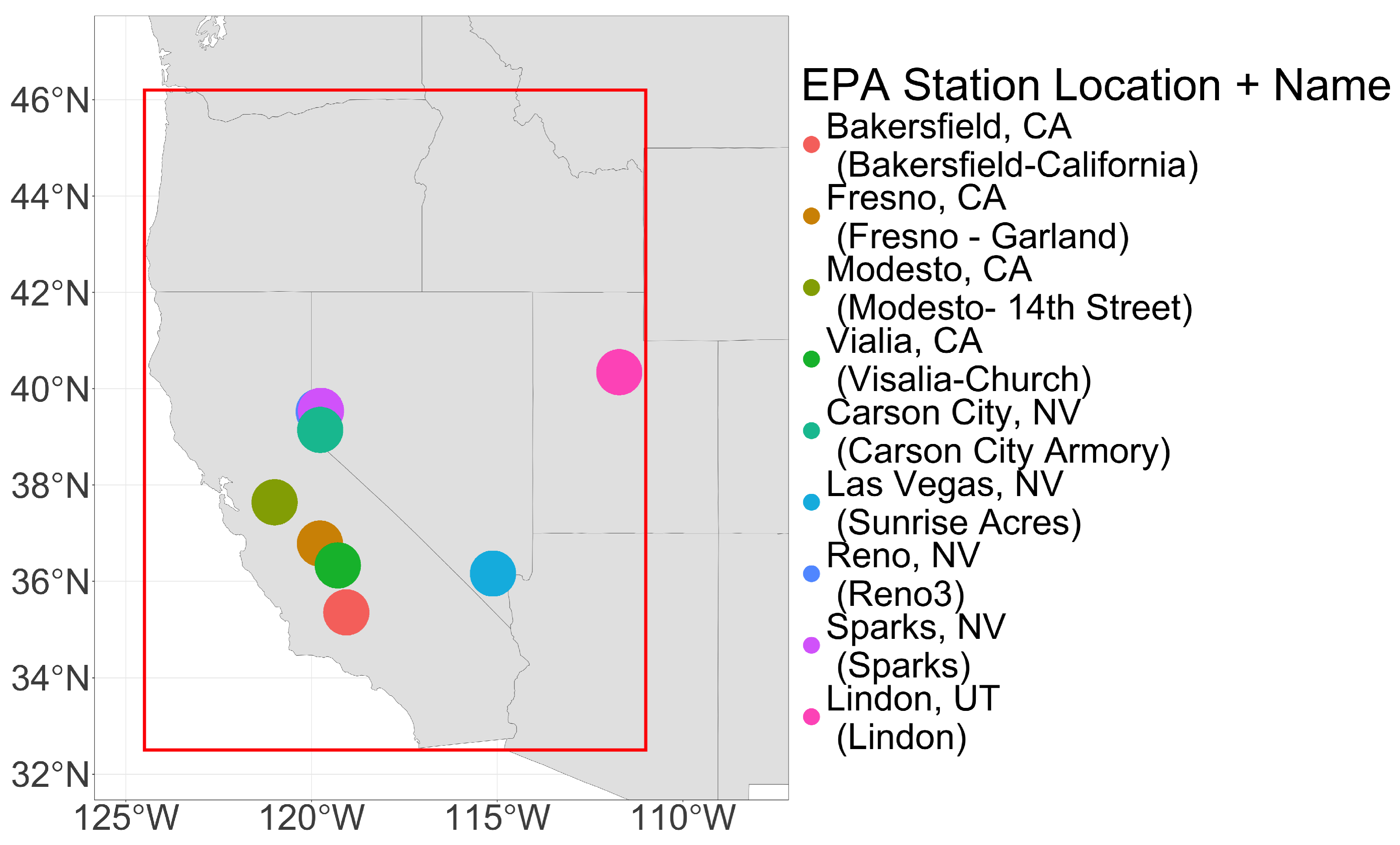
EPA ground-based air pollution monitors provide an external comparison dataset (EPA dataset 88101 [34]). The EPA data came from eight locations in California and Nevada: Bakersfield, CA; Fresno, CA; Modesto, CA; Visalia, CA; Carson City, NV; Las Vegas, NV; Reno, NV; and Sparks, NV. These monitors were chosen because they are directly downwind of major fire sources. Both the EPA monitoring data and the HYSPLIT output are associated with the static 12 km NAM grid. To ensure consistent spatial alignment, EPA monitor locations are matched to their nearest NAM grid cell, and only HYSPLIT concentrations from that same grid cell are used for comparison. This method avoids large spatial mismatches and ensures that model-to-observation comparisons are made within the same gridded domain. The EPA monitors capture daily PM_2.5 measurements at ground level; however, these measurements are not directly comparable to the HYSPLIT results, because the EPA monitors capture PM_2.5 from all sources (e.g., cars, industrial pollution), while the HYSPLIT results are smoke-specific.

NASA WorldView visible satellite imagery [35] also serves as a valuable evaluation dataset for assessing HYSPLIT smoke dispersion modeling results. These images provide a visual record of wildfire locations, smoke plume extent, and transport patterns, allowing for qualitative comparisons between observed smoke movement and model predictions. By comparing a map of HYSPLIT ambient concentrations with the visual images captured by WorldView, this imagery can be used to evaluate how well HYSPLIT captures the spatial distribution wildfire smoke. WorldView does not provide direct concentration measurements.

3. Results and Discussion

This section analyzes the performance of different FEIs as inputs to the HYSPLIT PM_2.5 dispersion results in addition to comparing the HYSPLIT results to EPA ground-based PM_2.5 monitoring information and visible satellite imagery. Domain-wide annual averages of the HYSPLIT PM_2.5 concentration results at the 10 m atmospheric layer are used to analyze differences between FEIs over a large spatial and temporal domain. Differences in the vertical distribution of HYSPLIT concentrations are also examined because vertical distribution of PM_2.5 impacts particulate transport. The comparisons between EPA monitoring data and HYSPLIT concentrations are performed on a domain-wide basis and at each individual station. Finally, results for large wildfires are presented to examine the differences between FEIs on a shorter time scale. The shorter time scale allows for qualitative evaluation of visual satellite images, which would be impossible over the entire study period.

3.1. Atmospheric Dispersion Modeling Results for Each FEI

FEI_COMBO increases domain-wide total annual smoke PM_2.5 concentration in the HYSPLIT 10 m as layer compared to HYSPLIT over FEI_BASE (

Table 2. HYSPLIT PM_2.5 ambient concentrations in $\mathsf{\mu }\mathrm{g}{\mathrm{m}}^{-3}$ vertically allocated at four atmospheric levels for each year and fire emission inventory.

Year	FEI	10 m PM2.5 ($\mathsf{\mu }\mathbf{g}{\mathbf{m}}^{-3}$)	100 m PM2.5 ($\mathsf{\mu }\mathbf{g}{\mathbf{m}}^{-3}$)	1000 m PM2.5 ($\mathsf{\mu }\mathbf{g}{\mathbf{m}}^{-3}$)	5000 m PM2.5 ($\mathsf{\mu }\mathbf{g}{\mathbf{m}}^{-3}$)	Total Column PM2.5 ($\mathsf{\mu }\mathbf{g}{\mathbf{m}}^{-3}$)
2013	BASE	$4.17\times {10}^6$	$3.31\times {10}^6$	$8.64\times {10}^5$	$1.37\times {10}^4$	$8.36\times {10}^6$
2013	COMBO	$6.67\times {10}^6$	$5.46\times {10}^6$	$1.37\times {10}^6$	$1.78\times {10}^4$	$1.35\times {10}^7$
2013	COMBO+CC	$7.71\times {10}^6$	$6.30\times {10}^6$	$1.61\times {10}^6$	$2.32\times {10}^4$	$1.56\times {10}^7$
2016	BASE	$2.24\times {10}^6$	$1.95\times {10}^6$	$6.05\times {10}^5$	$4.95\times {10}^4$	$4.85\times {10}^6$
2016	COMBO	$3.19\times {10}^6$	$2.76\times {10}^6$	$8.34\times {10}^5$	$6.81\times {10}^4$	$6.86\times {10}^6$
2016	COMBO+CC	$3.51\times {10}^6$	$3.00\times {10}^6$	$8.93\times {10}^5$	$7.63\times {10}^4$	$7.48\times {10}^6$
2018	BASE	$9.79\times {10}^6$	$8.37\times {10}^6$	$1.99\times {10}^6$	$4.81\times {10}^4$	$2.02\times {10}^7$
2018	COMBO	$1.41\times {10}^7$	$1.21\times {10}^7$	$2.75\times {10}^6$	$5.99\times {10}^4$	$2.90\times {10}^7$
2018	COMBO+CC	$1.51\times {10}^7$	$1.29\times {10}^7$	$2.97\times {10}^6$	$7.20\times {10}^4$	$3.11\times {10}^7$

). FEI_COMBO+CC also provides an additional increase over FEI_COMBO. In the three years analyzed, FEI_COMBO provides approximately a 5% increase in the number of PM_2.5 concentration points over FEI_BASE, and FEI_COMBO+CC provides approximately a 25% increase in the number of grid cells with non-zero HYSPLIT-modeled PM_2.5 concentrations. In 2013, FEI_COMBO+CC provides more grid cells with non-zero HYSPLIT-modeled PM_2.5 concentration, more days with 10 m PM_2.5 concentration, and a higher total PM_2.5 concentration.

In 2016, FEI_COMBO+CC provides more days and locations with PM_2.5 concentration than FEI_BASE and FEI_COMBO (Table 2). FEI_COMBO provided fewer fire than the FEI_BASE. This could be caused by satellite remote sensing issues like cloud cover and could be specific to 2016. Increased emissions may be lofted higher in the atmosphere and thus do not accumulate in the 10 m atmospheric concentration layer (Table 2). The total annual PM_2.5 concentration for both FEI_COMBO+CC and FEI_COMBO is higher than the yearly concentration from FEI_BASE. However, FEI_COMBO+CC has a lower annual concentration than FEI_COMBO despite having more days with PM_2.5 concentration. This exemplifies that the cloud cover algorithm primarily includes information from low intensity fire days at the beginning or end of a fire, because the emissions are spread over more days. More days of small fires means a higher frequency of low emissions that are dispersed through the atmosphere. These lower emission days are likely not lofted as high into the atmosphere by the dispersion model, meaning they are more prevalent at the 10 m height (Table 2).

For 2018, FEI_COMBO+CC provided more days with PM_2.5 concentration and more annual total PM_2.5 concentration over both FEI_BASE and FEI_COMBO (Table 1). FEI_COMBO and FEI_BASE have the same number of days with PM_2.5 concentration, but FEI_COMBO provides more total annual concentration than FEI_BASE. This again exemplifies the changes made to FEI_COMBO, which includes additional fire information that increases the emissions, leading to increased concentration dispersed throughout the atmosphere on similar days to FEI_BASE.

The sums of the column-level PM_2.5 concentrations (Table 2) show that total modeled PM_2.5 increases substantially from FEI_BASE to FEI_COMBO and further to FEI_COMBO+CC, due to improve detection of fire activity and the addition of cloud corrected fire days. However, the vertical distribution of modeled concentrations remains relatively consistent across all three FEIs and years, with approximately 90% of the PM_2.5 concentrated below 1000 m, with nearly half of it in the 10 m level. While FEI_COMBO+CC does show a slightly higher total number of PM_2.5 concentration at the 5000 m level, the percentage remains small (less than 1% in all years), indicating that most smoke remains near the surface regardless of the FEI used. Additionally, the higher amount of modeled daily 10 m concentrations in FEI_COMBO+CC likely results from its more complete temporal coverage, reducing the number of missing smoke days.

The annual results show that FEI_COMBO+CC results in a greater number of grid cells with non-zero HYSPLIT-modeled PM_2.5 concentrations compared to the other emissions inventories. FEI_COMBO also increases coverage relative to FEI_BASE, but FEI_COMBO+CC consistently provides the most additional information. The expanded spatial and temporal fire emission data included in FEI_COMBO+CC leads to broader dispersion of PM_2.5 throughout the modeling domain Additionally, FEI_COMBO+CC frequently produces higher daily 10 m PM_2.5 concentrations, suggesting it captures fire activity that the other inventories miss. These improvements are particularly valuable for acute research on health effects, as missing concentration estimates on individual days can lead to underestimation of short-term exposure and ultimately affect epidemiological findings.

3.2. EPA Comparison

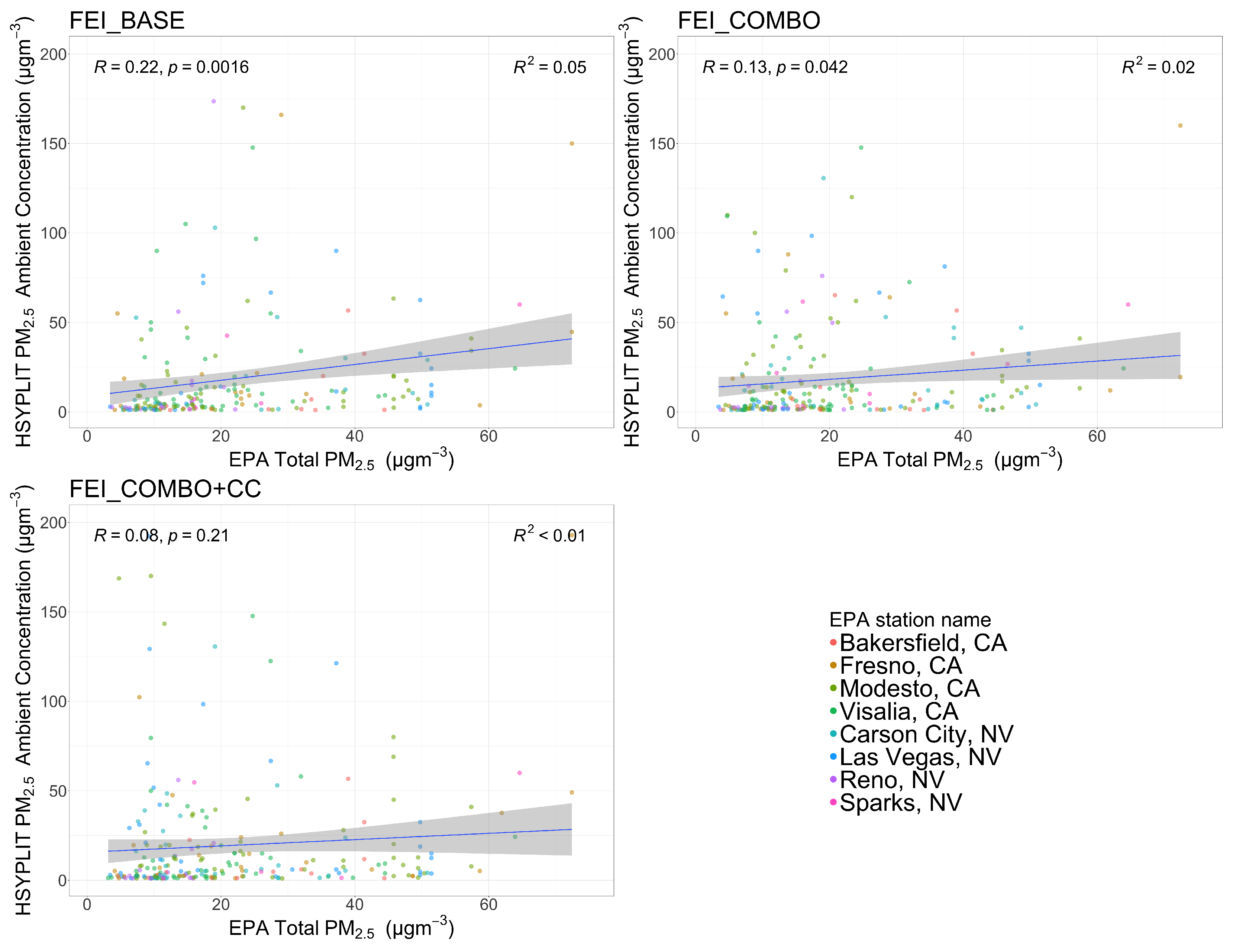
Comparing HYSPLIT outputs with EPA measurements offers insight into how well the model may be capturing real-world smoke transport patterns. For 2013, FEI_COMBO+CC had the highest annual domain-wide correlation (R = 0.36) and the lowest p-value (p < 0.01) (Figure 2). In 2016, the p-value was statistically significant for both the combination and cloud cover FEIs but not for the MODIS FEI, though the correlations are not as strong for 2016 (Figure 3). In 2018, the correlations between the FEIs and EPA values are not statistically significant, aside from the FEI_BASE, which does not show a strong correlation (Figure 4). This could be due to many reasons, including the fact that the EPA data specifically captures PM_2.5 pollution from sources other than fire smoke. This also means that the NMB and RMSE values can only be compared between the FEIs, and cannot be used quantitatively, because the EPA data is not smoke specific. Additionally, because EPA monitors capture emissions measurements at a single location with narrow spatial coverage, there are numerous reasons that HYSPLIT may not capture the same trend. EPA monitors are highly localized, and HYSPLIT operates on a larger regional scale that may not capture the localized topography or meteorological conditions near the EPA monitor that impacts the PM_2.5 measurements.

A further comparison of EPA monitor data and HYSPLIT concentrations using normalized mean bias (NMB) and root mean squared error (RMSE) provides more information on the relationship between the simulation HYSPLIT PM_2.5 concentration data and the measured EPA PM_2.5 data (

Table 3. The domain-wide normalized mean bias (%), domain-wide RMSE in $\mathsf{\mu }\mathrm{g}{\mathrm{m}}^{-3}$ for each year and FEI, and domain-wide correlation based on HYSPLIT PM_2.5 concentrations and EPA measured PM_2.5 concentrations. Note: EPA measurements are not wildfire smoke specific and includes PM_2.5 from all sources.

Year	FEI	NMB (%)	RMSE ($\mathsf{\mu }$g)	Correlation
2013	BASE	11.13	24.52	0.30
2013	COMBO	10.99	26.05	0.28
2013	COMBO + CC	10.73	27.26	0.28
2016	BASE	9.62	11.59	0.05
2016	COMBO	9.29	14.99	0.06
2016	COMBO + CC	9.19	14.90	0.07
2018	BASE	11.38	16.91	0.16
2018	COMBO	11.16	18.58	0.09
2018	COMBO + CC	10.96	19.24	0.09

). NMB measures whether HYSPLIT is over-predicting or under-predicting PM_2.5 and uses the EPA data as ground-truth for comparison. For each year, the FEI_BASE had the highest domain-wide NMB of the FEIs (11.13, 9.62, 11.38), meaning that FEI_BASE consistently overestimates PM_2.5 compared to measured EPA data. The FEI_COMBO+CC had the lowest domain-wide NMB of all the FEIs (10.73, 9.19, 10.96) for each year, meaning that FEI_COMBO+CC consistently estimated PM_2.5 better than FEI_BASE or FEI_COMBO. However, FEI_COMBO+CC also consistently overestimated PM_2.5, because the NMB is consistently high. HYSPLIT may overestimate PM_2.5 concentrations due to several favors, including inherent uncertainties in emissions estimates. Applying a bias correction to HYSPLIT-modeled PM_2.5 before using it health effect studies can improve alignment with observed PM_2.5 measurements [12].

When looking at RMSE, the opposite trend is seen. For each year, FEI_BASE had the lowest domain-wide RMSE of the FEIs (24.52, 11.59, 16.91), meaning that, on average, the FEI_BASE is closer to the EPA PM_2.5 values than the other FEIs. The FEI_COMBO+CC has the highest domain-wide RMSE for all years (27.26, 14.99, 19.24). FEI_COMBO+CC and FEI_COMBO HYSPLIT PM_2.5 concentration results have on average, higher RMSE and are less representative of the EPA-measured PM_2.5 values than FEI_BASE. Looking at both the NMB and the RMSE reveals that FEI_COMBO+CC tends to be closer to the EPA PM_2.5 values (low bias), but the individual difference between two PM_2.5 values from HYSPLIT and the EPA monitors can still be quite large (high RMSE). Due to the extremely variable nature of fire behavior and the challenges associated with comparing HYSPLIT and EPA data, a large variance between individual PM_2.5 measurements is unsurprising, which can be very difficult to fit in a model, leading to a high RMSE.

Looking at the NMB and RMSE (

Table 4. Bakersfield, CA, site-specific normalized mean bias (%), domain-wide RMSE in $\mathsf{\mu }\mathrm{g}{\mathrm{m}}^{-3}$ for each year and FEI, and domain-wide correlation based on HYSPLIT PM_2.5 concentrations and EPA measured PM_2.5 concentrations.

Year	FEI	NMB (%)	RMSE ($\mathsf{\mu }$g)	Correlation
2013	BASE	16.46	20.48	0.08
2013	COMBO	16.55	20.46	0.17
2013	COMBO + CC	16.63	20.53	0.25
2016	BASE	12.81	14.90	0.00
2016	COMBO	12.69	15.25	−0.01
2016	COMBO + CC	12.71	15.25	0.00
2018	BASE	14.67	18.17	0.14
2018	COMBO	14.59	18.24	0.11
2018	COMBO + CC	14.63	18.15	0.13

,

Table 5. Carson City, NV, site-specific normalized mean bias (%), domain-wide RMSE in $\mathsf{\mu }\mathrm{g}{\mathrm{m}}^{-3}$ for each year and FEI, and domain-wide correlation based on HYSPLIT PM_2.5 concentrations and EPA measured PM_2.5 concentrations.

Year	FEI	NMB (%)	RMSE ($\mathsf{\mu }$g)	Correlation
2013	BASE	8.19	42.37	0.45
2013	COMBO	8.76	42.50	0.44
2013	COMBO + CC	8.01	38.34	0.46
2016	BASE	4.89	6.19	0.07
2016	COMBO	4.56	9.17	0.05
2016	COMBO + CC	4.80	6.23	0.05
2018	BASE	10.31	17.69	0.16
2018	COMBO	10.40	17.47	0.15
2018	COMBO + CC	10.24	17.48	0.19

,

Table 6. Fresno, CA, site-specific normalized mean bias (%), domain-wide RMSE in $\mathsf{\mu }\mathrm{g}{\mathrm{m}}^{-3}$ for each year and FEI, and domain-wide correlation based on HYSPLIT PM_2.5 concentrations and EPA measured PM_2.5 concentrations.

Year	FEI	NMB (%)	RMSE ($\mathsf{\mu }$g)	Correlation
2013	BASE	14.03	18.16	−0.03
2013	COMBO	13.99	18.13	−0.03
2013	COMBO + CC	13.60	19.47	0.00
2016	BASE	11.78	13.53	0.08
2016	COMBO	11.29	15.01	0.16
2016	COMBO + CC	10.88	15.46	0.16
2018	BASE	13.05	17.92	0.14
2018	COMBO	12.69	18.34	0.08
2018	COMBO + CC	12.17	22.86	0.05

,

Table 7. Las Vegas, NV, site-specific normalized mean bias (%), domain-wide RMSE in $\mathsf{\mu }\mathrm{g}{\mathrm{m}}^{-3}$ for each year and FEI, and domain-wide correlation based on HYSPLIT PM_2.5 concentrations and EPA measured PM_2.5 concentrations.

Year	FEI	NMB (%)	RMSE ($\mathsf{\mu }$g)	Correlation
2013	BASE	7.87	24.91	0.09
2013	COMBO	7.85	25.64	0.09
2013	COMBO + CC	8.12	22.48	0.09
2016	BASE	10.29	12.20	0.05
2016	COMBO	10.35	12.04	0.05
2016	COMBO + CC	10.14	12.23	0.01
2018	BASE	8.04	11.11	0.10
2018	COMBO	8.13	9.97	0.12
2018	COMBO + CC	8.24	9.72	0.08

,

Table 8. Modesto, CA, site-specific normalized mean bias (%), domain-wide RMSE in $\mathsf{\mu }\mathrm{g}{\mathrm{m}}^{-3}$ for each year and FEI, and domain-wide correlation based on HYSPLIT PM_2.5 concentrations and EPA measured PM_2.5 concentrations.

Year	FEI	NMB (%)	RMSE ($\mathsf{\mu }$g)	Correlation
2013	BASE	12.24	16.25	0.00
2013	COMBO	11.89	16.43	0.00
2013	COMBO + CC	11.96	16.58	0.01
2016	BASE	10.85	12.35	−0.01
2016	COMBO	10.73	12.23	0.08
2016	COMBO + CC	10.66	12.34	0.03
2018	BASE	11.88	20.57	0.22
2018	COMBO	11.21	27.91	0.09
2018	COMBO + CC	11.29	23.82	0.14

,

Table 9. Reno, NV, site-specific normalized mean bias (%), domain-wide RMSE in $\mathsf{\mu }\mathrm{g}{\mathrm{m}}^{-3}$ for each year and FEI, and domain-wide correlation based on HYSPLIT PM_2.5 concentrations and EPA measured PM_2.5 concentrations.

Year	FEI	NMB (%)	RMSE ($\mathsf{\mu }$g)	Correlation
2013	BASE	9.34	17.70	0.34
2013	COMBO	8.06	26.89	0.24
2013	COMBO + CC	9.07	20.68	0.30
2016	BASE	7.37	8.59	0.18
2016	COMBO	7.30	8.70	0.02
2016	COMBO + CC	7.30	8.69	0.03
2018	BASE	11.00	15.73	0.10
2018	COMBO	10.83	15.75	0.13
2018	COMBO + CC	10.84	16.01	0.05

,

Table 10. Sparks, NV, site-specific normalized mean bias (%), domain-wide RMSE in $\mathsf{\mu }\mathrm{g}{\mathrm{m}}^{-3}$ for each year and FEI, and domain-wide correlation based on HYSPLIT PM_2.5 concentrations and EPA measured PM_2.5 concentrations.

Year	FEI	NMB (%)	RMSE ($\mathsf{\mu }$g)	Correlation
2013	BASE	9.65	23.68	0.23
2013	COMBO	9.90	25.47	0.18
2013	COMBO + CC	7.85	42.35	0.25
2016	BASE	7.12	8.28	0.01
2016	COMBO	6.81	8.71	−0.02
2016	COMBO + CC	6.77	8.71	−0.03
2018	BASE	9.91	14.72	0.20
2018	COMBO	9.85	15.23	0.10
2018	COMBO + CC	9.43	16.61	0.08

and

Table 11. Visalia, CA, site-specific normalized mean bias (%), domain-wide RMSE in $\mathsf{\mu }\mathrm{g}{\mathrm{m}}^{-3}$ for each year and FEI, and domain-wide correlation based on HYSPLIT PM_2.5 concentrations and EPA measured PM_2.5 concentrations.

Year	FEI	NMB (%)	RMSE ($\mathsf{\mu }$g)	Correlation
2013	BASE	13.67	18.08	0.05
2013	COMBO	13.03	18.13	0.09
2013	COMBO + CC	13.01	17.63	0.14
2016	BASE	13.11	14.79	0.21
2016	COMBO	10.21	41.73	0.12
2016	COMBO + CC	9.91	41.71	0.12
2018	BASE	15.35	18.97	0.23
2018	COMBO	14.02	24.78	0.09
2018	COMBO + CC	12.29	33.36	0.07

) at each EPA monitoring location can provide insight to how the HYSPLIT performs at different locations. The Nevada stations tend to have better correlation with the EPA data, meaning that the HYSPLIT results are better correlated with the EPA data after transport through the atmosphere. This can be due to the background meteorology of each location, with some locations in California being prone to higher pollution due to agriculture [36]. This could also be related to atmospheric mixing dynamics close to the fire [37]. FEI_BASE typically shows higher NMB values, meaning it may overestimate PM_2.5 compared to the other inventories. This overestimation may be influenced by missing data points, as FEI_BASE has less small fire activity than the other inventories, leading to missing points that cannot be compared between the inventories. These missing points can potentially create an artificial improvement in performance for FEI_BASE. Also, because FEI_BASE does not contain the data points that are missed, which is a main reason that the two additional FEIs were developed, the missing days could influence the trends for FEI_BASE and artificially give better evaluation metrics (lower RMSE). Additionally, 2018 shows more variability across all locations, meaning that it was more difficult to capture with the HYSPLIT model. Prior to 2020, 2018 was a historic fire year with some of the largest fires in the western US [38], providing insight to the difficulties of modeling that year and the additional models that will be faced under a changing climate.

Overall, no single FEI outperforms the others in all years and locations, exemplifying the difficulty of modeling wildfire smoke in the western US. However, the combination and cloud cover FEIs show more balanced performance, while using WFEIS leads to higher biases. This means that the improvements to the FEIs do provide benefit. The cloud cover FEI often produces less extreme bias than WFEIS and shows higher correlation values, making it a reasonable choice for larger modeling efforts to estimate health effects of PM_2.5 from smoke.

Comparing the results of atmospheric dispersion models when using different fire input information helps quantify the differences that occur when using different FEIs. Quantifying these differences helps provide comparability between health effect studies, which often use different fire information and reach disparate conclusions on the effects of PM_2.5 on human health [39,40]. Because the variations in the FEIs used in this study reflect enhancements aimed at addressing FEI challenges, they provide insight into how these challenges may affect fire dispersion modeling.

3.3. Large Fire Case Studies

Three large fires provide an opportunity to examine the differences in dispersion modeling results between different input FEIs in depth, over a shorter time. The number of concentration locations (Lagrangian grid cells with a non-zero PM_2.5 concentration estimated by HYSPLIT) determined by each FEI at each fire are compared, along with a comparison of concentration maps from HYSPLIT and visible satellite images, providing a spatial understanding of differences between FEIs. Comparison between the HYSPLIT results using different FEIs and EPA monitoring data also provides additional information about how the FEIs compare to real-world data.

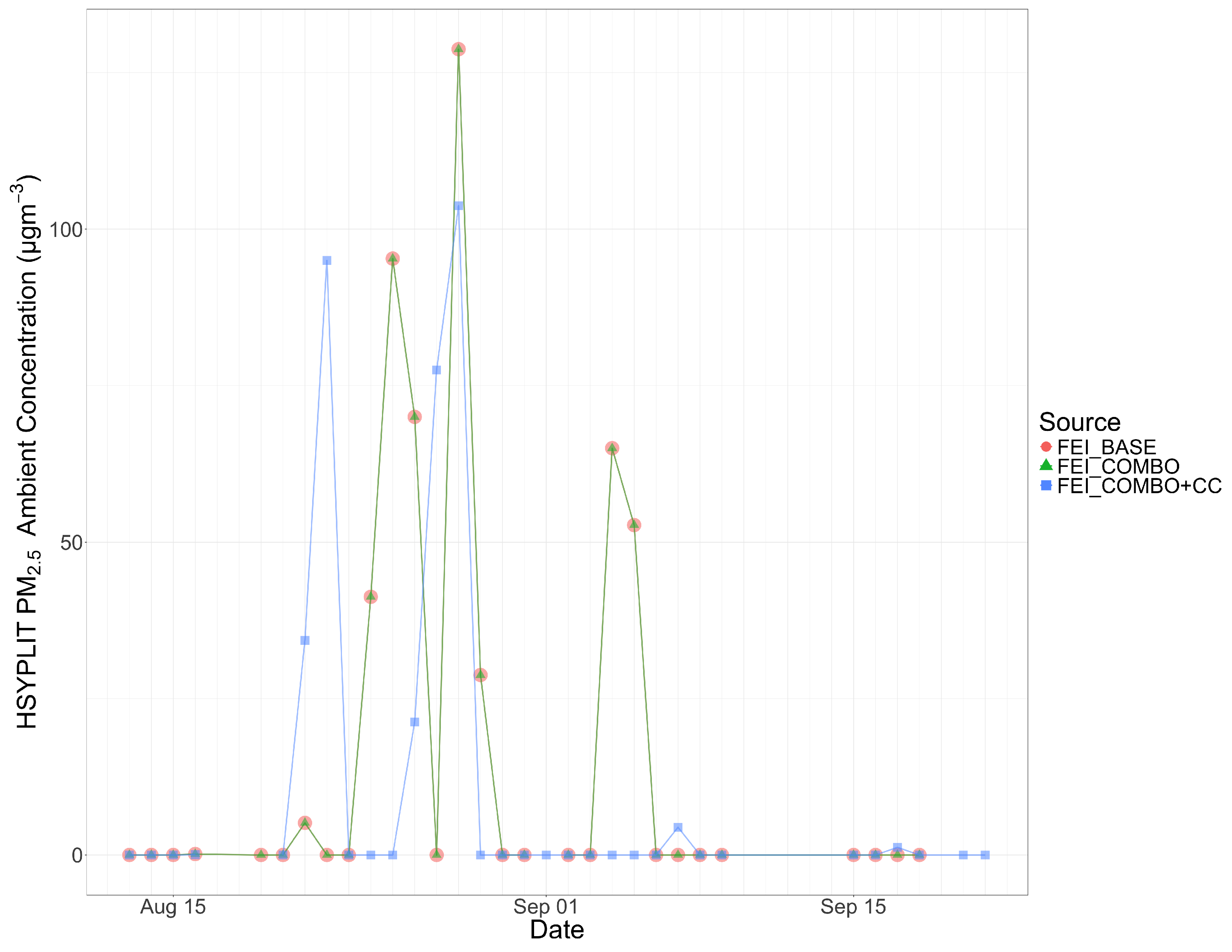
The Rim Fire in 2013 had the least number of different concentration locations between different emissions inventories (

Table 12. The number of fire days, total annual PM_2.5 concentrations in kg from HYSPLIT over the entire domain, and the percent increase in the number of locations with downwind PM_2.5 concentration estimated by HYSPLIT between FEIs. Note that there may be more than one fire per day.

Year	FEI	Fire Days	Annual 10 m PM2.5 Concentrations (kg)	% Increase in Concentrations	% Increase in Downwind Locations
2013	BASE	284	$6.57\times {10}^3$	–	–
2013	COMBO	286	$7.05\times {10}^3$	7%	8%
2013	COMBO + CC	319	$7.90\times {10}^3$	12%	12%
2016	BASE	268	$1.24\times {10}^3$	–	–
2016	COMBO	245	$2.56\times {10}^3$	204%	0.4%
2016	COMBO + CC	285	$2.50\times {10}^3$	21%	22%
2018	BASE	301	$3.38\times {10}^3$	–	–
2018	COMBO	301	$6.31\times {10}^3$	35%	29%
2018	COMBO + CC	337	$1.00\times {10}^4$	23%	11%

). Additionally, the HYSPLIT concentration results for FEI_BASE and FEI_COMBO are the same for the Rim Fire, which means that FEI_BASE captured similar way FEI_COMBO. WFEIS MODIS and WFEIS MTBS were likely able to capture the Rim Fire well due to the large nature of the fire, but WFEIS MTBS does not provide daily fire progression, necessitating the FEI_COMBO. The Rim Fire has the largest PM_2.5 emissions and burned area of all three large fires examined. FEI_COMBO+CC was not the same as the other two FEIs and added approximately 0.5% different concentration points over the entire time of the Rim Fire. The Rim Fire time series (Figure 5) shows the same trends as the 2013 annual evaluation.

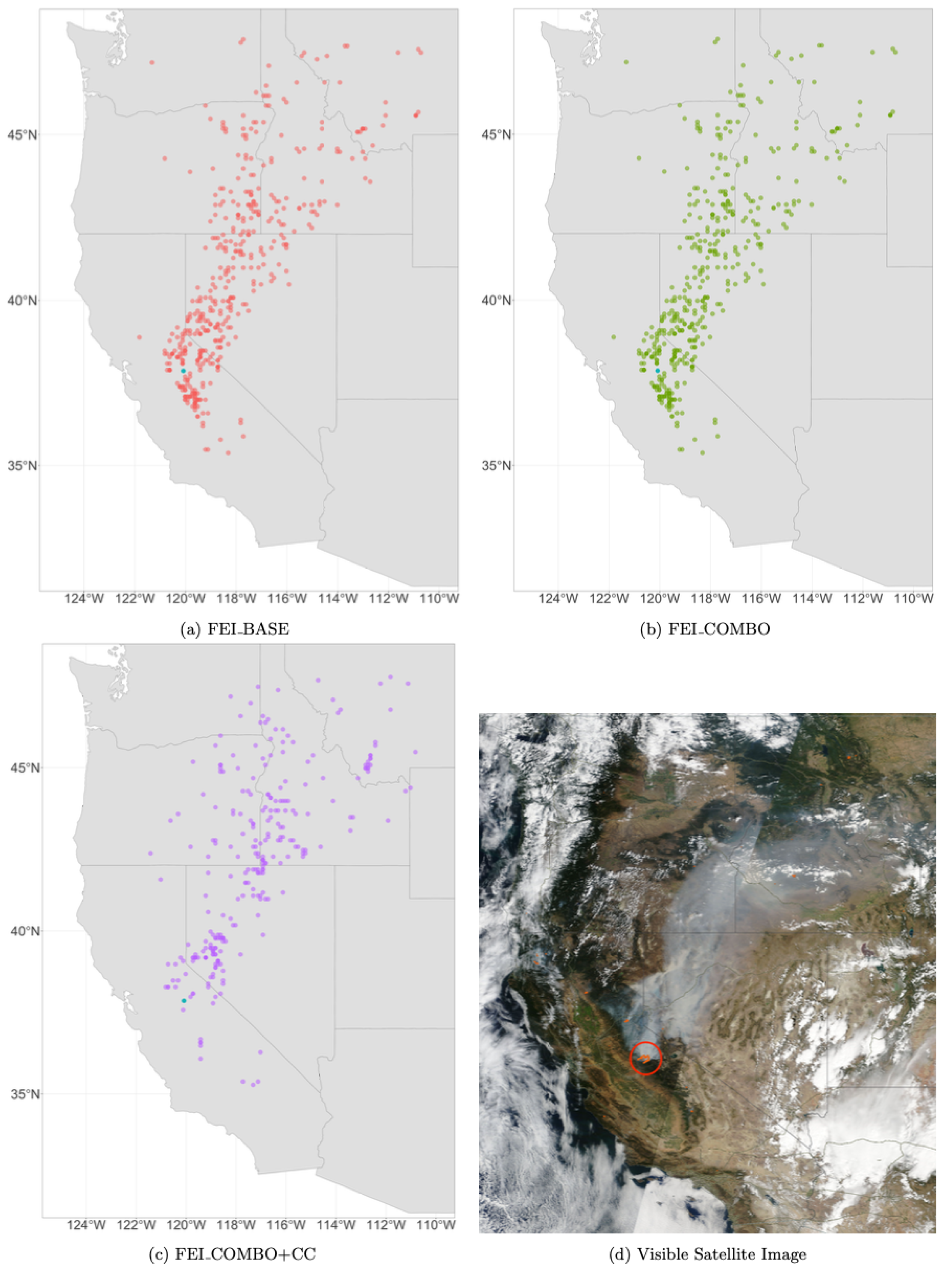
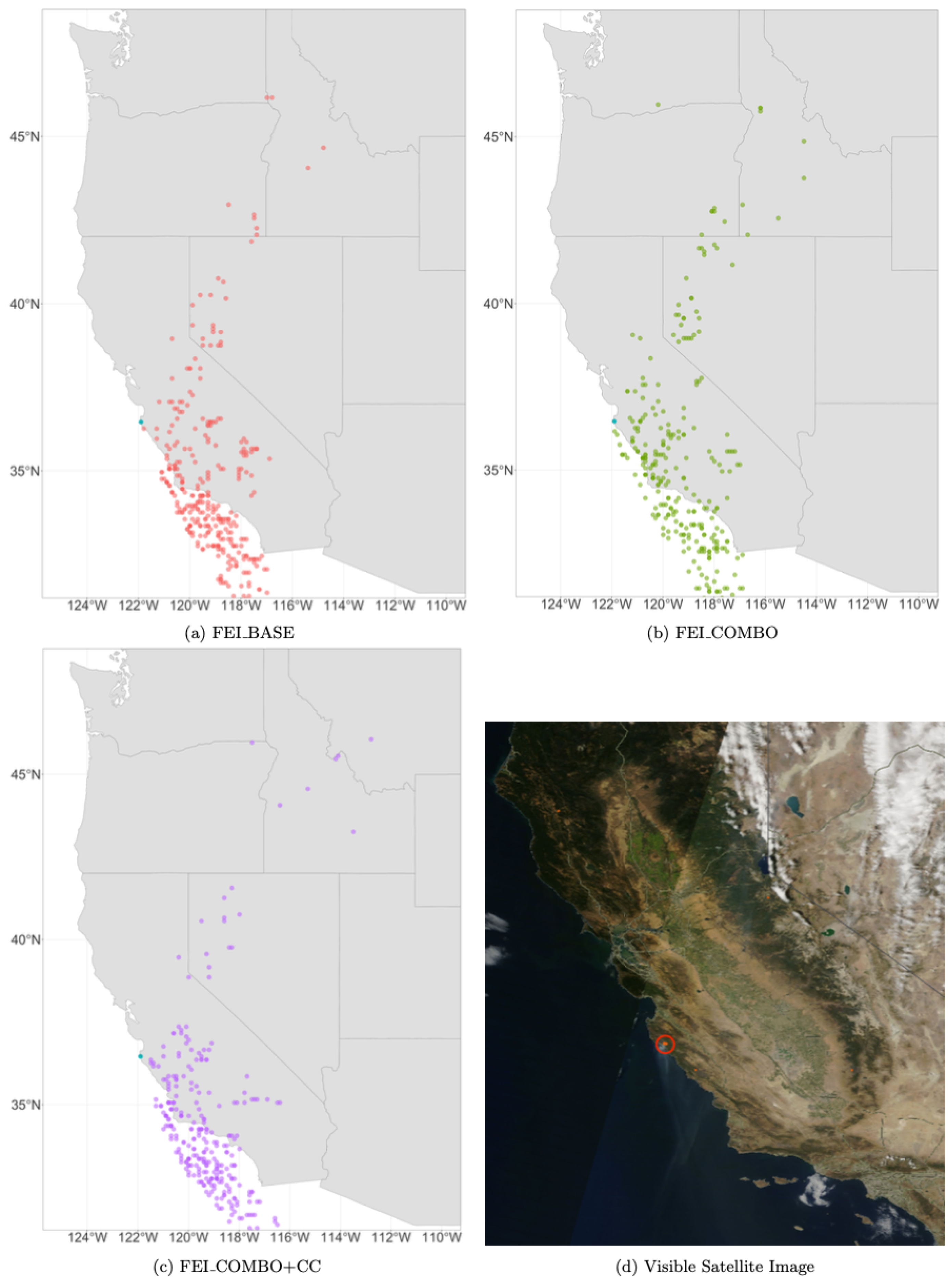
A comparison of HYSPLIT concentration results for a single day during the Rim Fire (24 August 2013) and satellite visible imagery from NASA WorldView provides additional insight into the difference that the FEIs create in dispersion modeling results. The HYSPLIT concentration maps (Figure 6) show that both the WFEIS FEI and the combination FEI provide the same results, likely because the Rim Fire was a large enough fire that the lower spatial resolution burned area product used in the WFEIS FEI was able to capture it. The satellite visible imagery of this day (Figure 6) shows the smoke plume from the Rim Fire being transported to the north-east. The HYSPLIT figure shows broadly the same dispersion pattern, with some variation that can be attributed to the HYSPLIT results representing the concentrations over the entire day and the visible image being a single snapshot in time. Additionally, in the visible image, smoke plume mixing is seen with another fire that is north of the Rim Fire. The HYSPLIT results do not reflect this smoke plume because the HYSPLIT ambient concentrations are specific to the Rim Fire. Fire-specific ambient concentrations from HYSPLIT allow for more information to be incorporated into health effect studies, providing information on how health effects relate to fire specific information like fire intensity and fuel type.

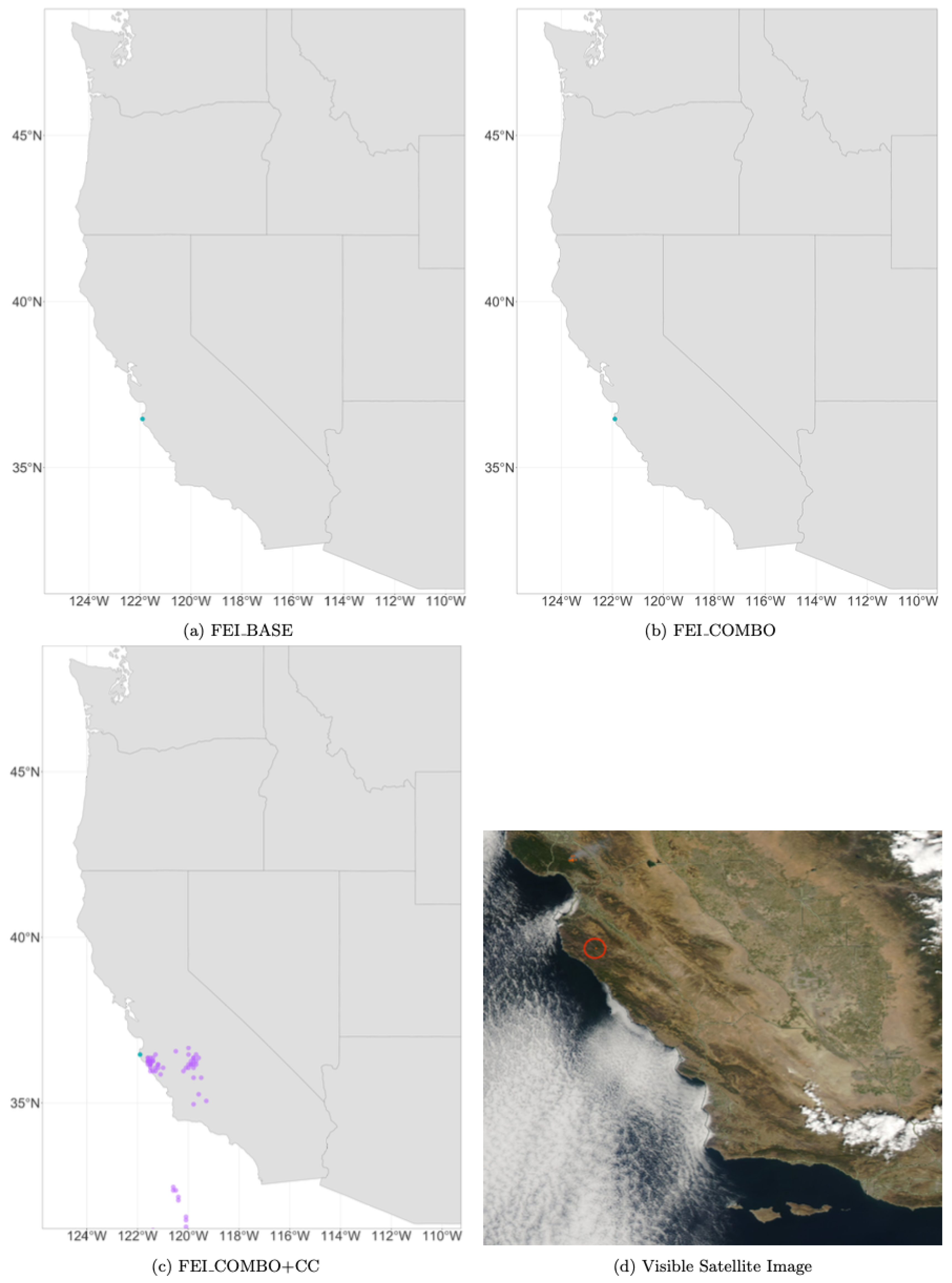
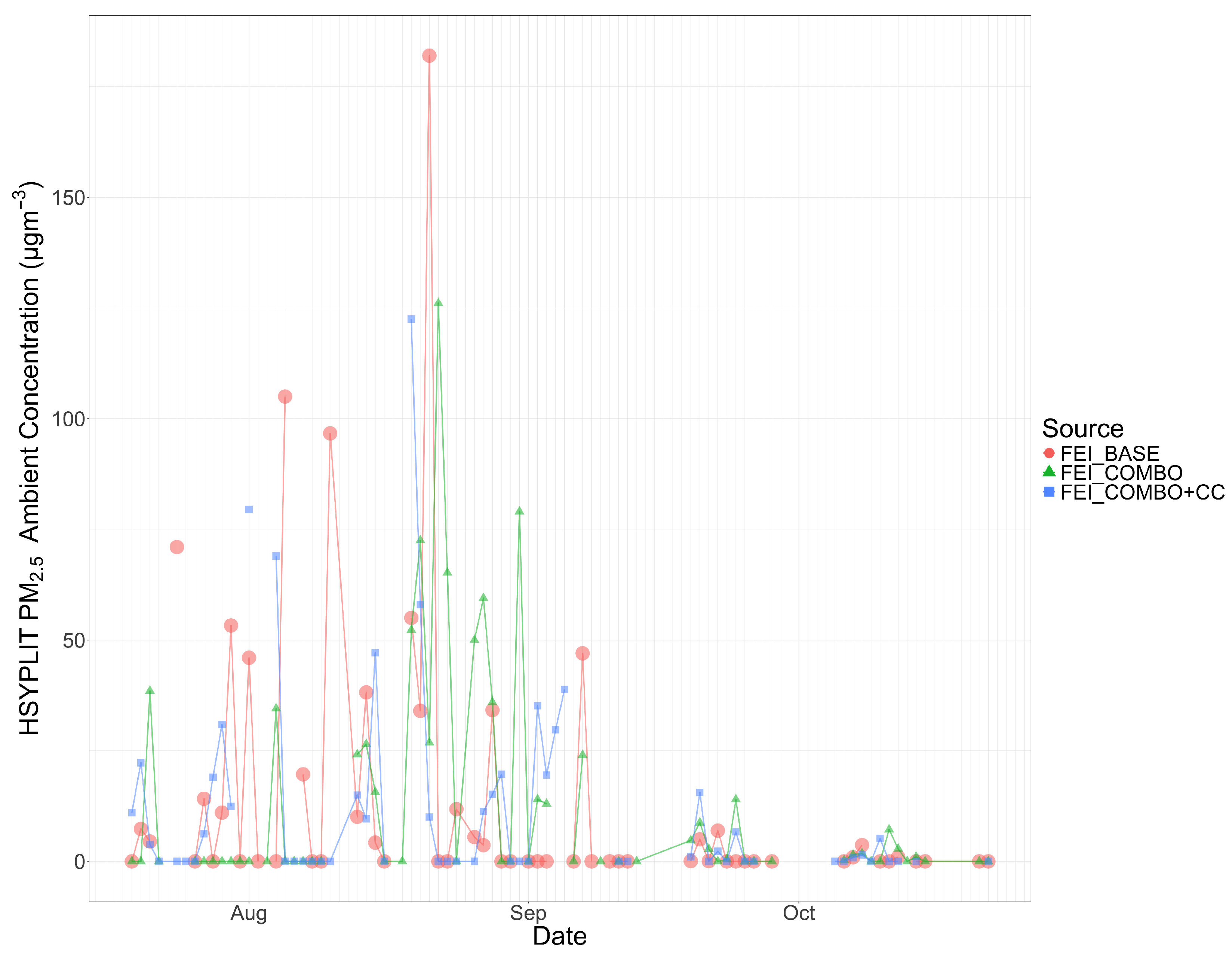
The Soberanes Fire in 2016 had a higher number of different concentration points than the Rim Fire and had the highest percentage of different concentration points (Table 12). The FEI_COMBO added about 0.2% different concentration points throughout the fire when compared to FEI_BASE, and FEI_COMBO+CC added about 0.01% different points. Because FEI_COMBO+CC primarily adds information on low fire intensity days at the beginning and end of a fire, to have a small amount of additional input from the FEI_COMBO+CC makes sense for a large fire. The results from FEI_BASE and FEI_COMBO were different for this fire, meaning that the combination provided additional concentration information for this fire. The time series of the Soberanes Fire (Figure 7) also shows the same trends as the 2016 annual comparison. Though the Soberanes Fire is large, it emitted less PM_2.5 and burned less area than the other two fire case studies presented in this analysis. The Soberanes Fire also lasted roughly 1.5 times longer than the Rim Fire, meaning that the Soberanes Fire produced less emissions and burned area over a longer period. This may indicate a lower fire intensity during the Soberanes Fire, which may cause more remote sensing issues that FEI_COMBO+CC can mitigate, like missed low intensity days at the beginning or end of a fire.

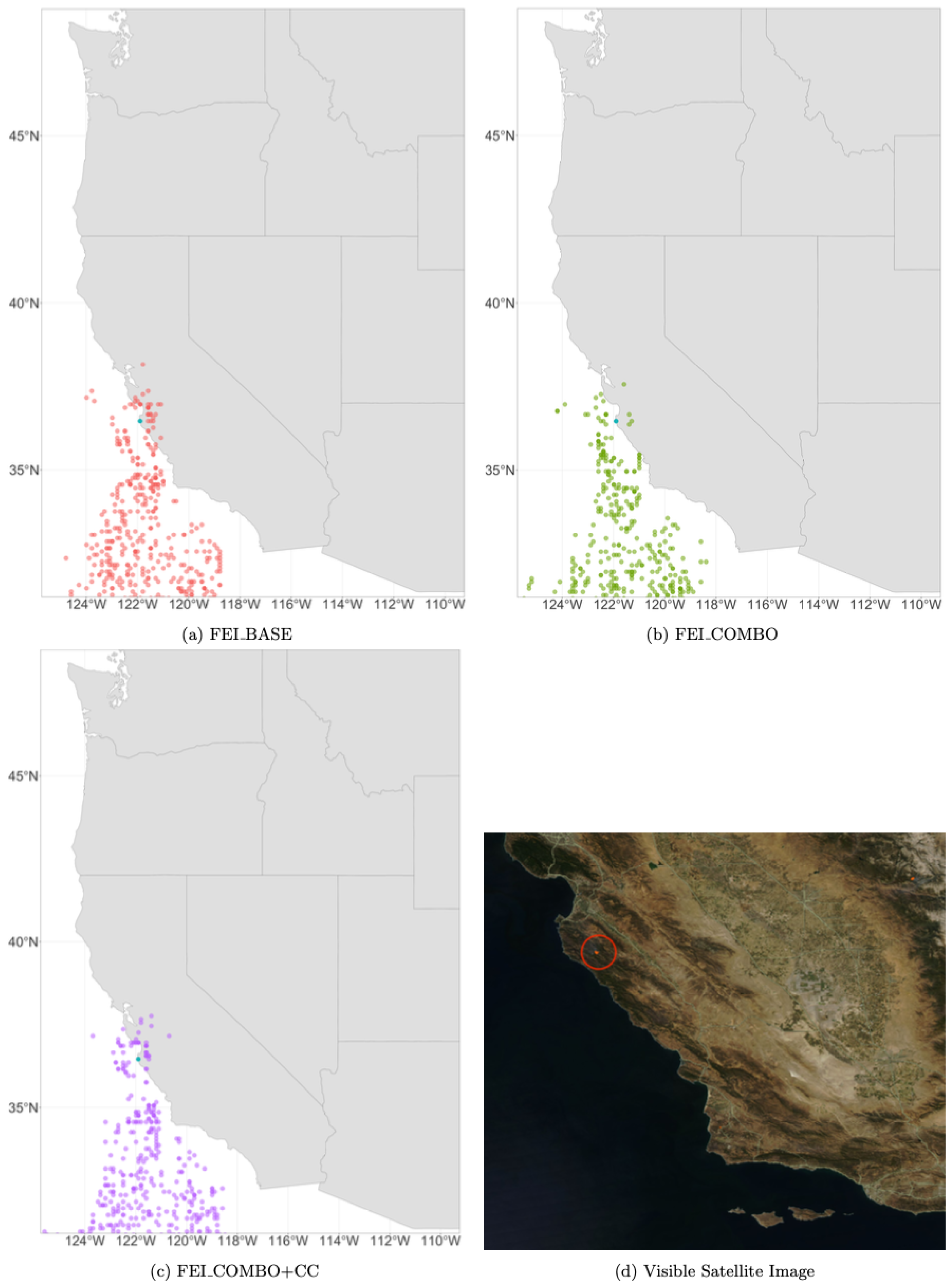
Comparison of a HYSPLIT concentration map for a single day (Figure 8) during the Soberanes Fire (30 August 2016) and NASA WorldView visible imagery (Figure 8) also shows broadly similar results between the two datasets. The visual images show a small plume of smoke being transported southwest over the Pacific Ocean. The HYSPLIT results show most of the concentration points in a similar southwestern direction. There are also numerous concentration points to the northeast in the HYSPLIT concentration map, which can represent a wind shift during the day that was not captured in the visible imagery. The differences between FEIs are more readily apparent in this HYSPLIT map compared to the Rim Fire, which suggests that differences between FEIs are more apparent in the dispersion results on lower emissions days.

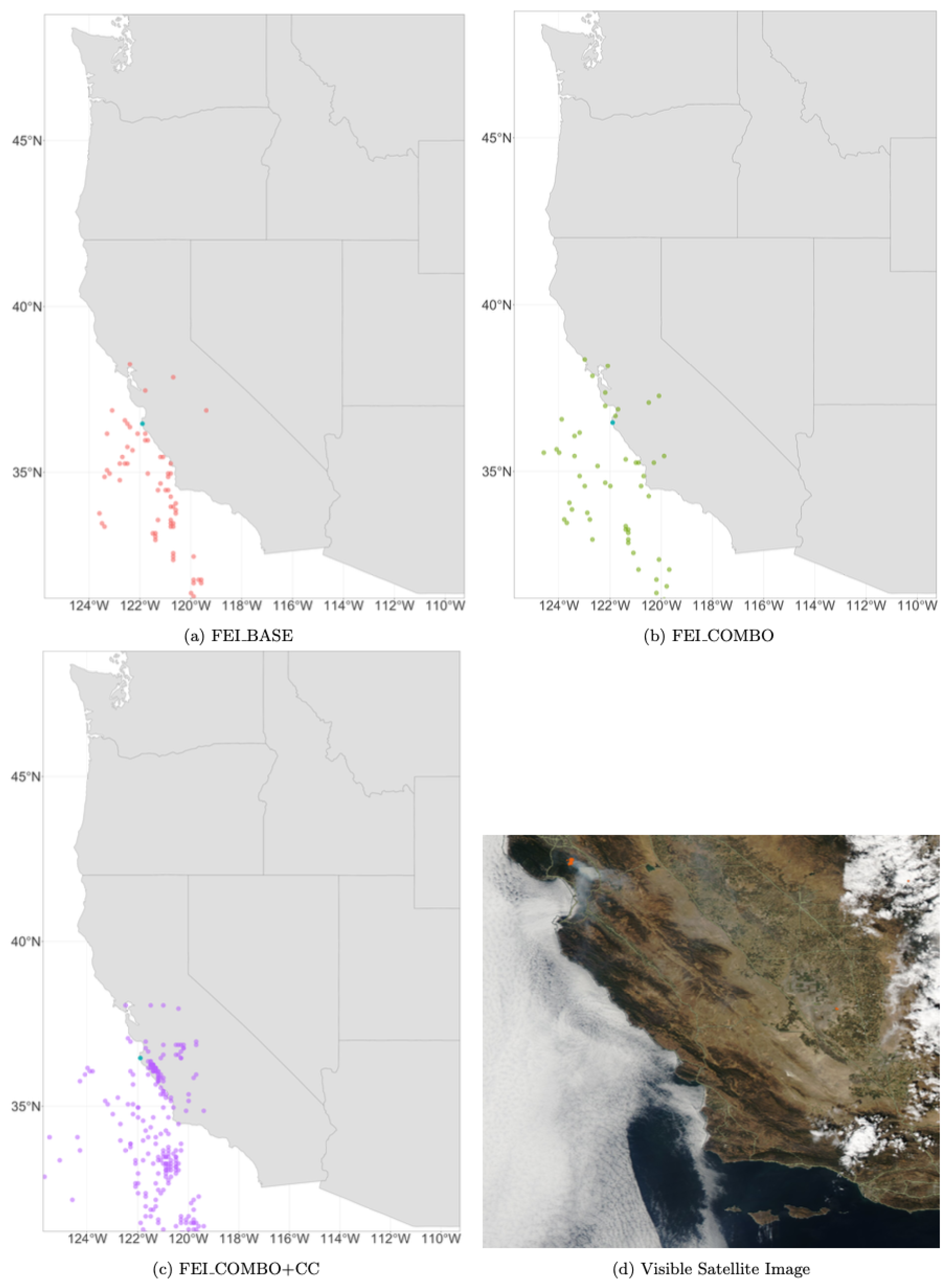
Additional examination of the Soberanes Fire shows how the HYSPLIT results using different FEIs can vary, particularly on lower emissions days. 26–29 September are days near the end of the Soberanes Fire, meaning they are lower in fire intensity and more difficult to sense remotely. The visual satellite image from 26 September (Figure 9) shows a single thermal anomaly sensed by MODIS, showing the low intensity of the fire at this point. On 26 September, all inventories and the visual satellite image capture the fire. On 27 September (Figure 10), all FEIs capture the fire, but the visual satellite image does not capture the fire. The same is true for 28 September (Figure 11), and on this day, the FEI_COMBO+CC results have a higher 10m PM_2.5 concentration. On 29 September (Figure 12), the fire is only captured by the FEI_COMBO+CC. Because MODIS is used to provide daily fire progression for FEI_COMBO, if MODIS doesn’t capture daily fire progression, then it cannot be assigned in the FEI_COMBO. Since there was an additional day captured in the FEI_COMBO+CC, these two missing days are interpolated in the FEI_COMBO+CC and thus concentration estimates are provided for this day. The two days that are captured in the FEI_COMBO+CC are the two non-consecutive days in the other FEIs (Table 1). Since acute health effects are short-lived in nature, the capture of these two days by the FEI_COMBO+CC provides additional information on daily concentrations that may impact human health.

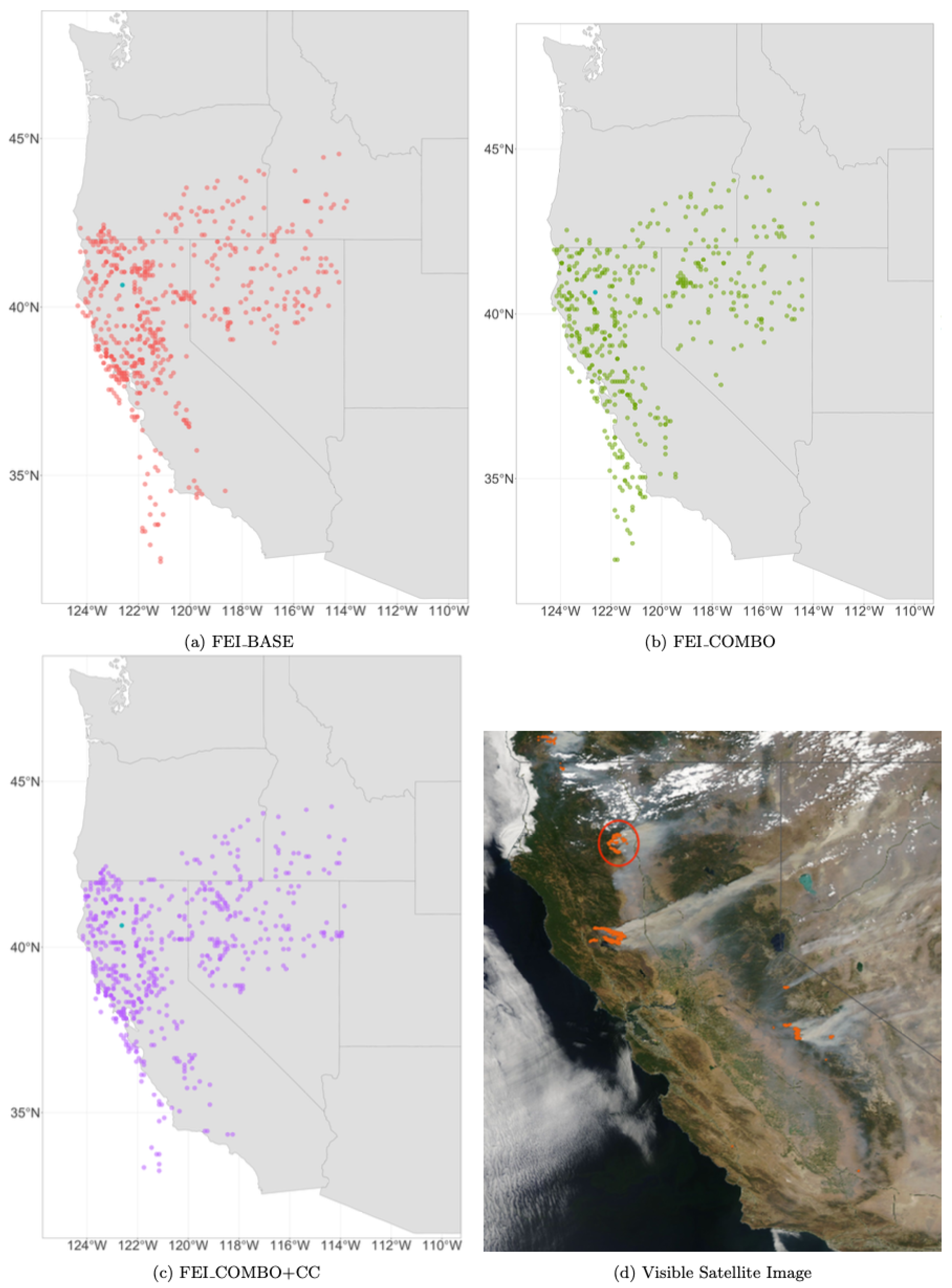
The Carr Fire in 2018 had more grid cells with non-zero HYSPLIT PM_2.5 concentrations than the other fires, but this was a lower percentage than the Soberanes Fire (Table 12). The large number of concentratoin points is related to the length of the fire (i.e., 101 days, Table 1). Since this was a large fire, there was more time for PM_2.5 to disperse through the atmosphere, and for the smoke to be advected away from the fire source. Therefore, the differences in HYSPLIT concentrations between FEIs were the most significant for this fire compared to the previous two fires discussed. The combination FEI added about 0.1% different concentration points, and the cloud cover FEI added about 0.5% different concentration points. Because this is a longer fire (Table 12), there is more chance for cloud cover that needs to be interpolated. The time series of the Carr Fire (Figure 13) shows the same trends as seen in the 2018 annual evaluation. This trend indicates that the cloud cover correction provide the greatest benefit for longer-duration fires, where gaps in satellite detection are more likely.

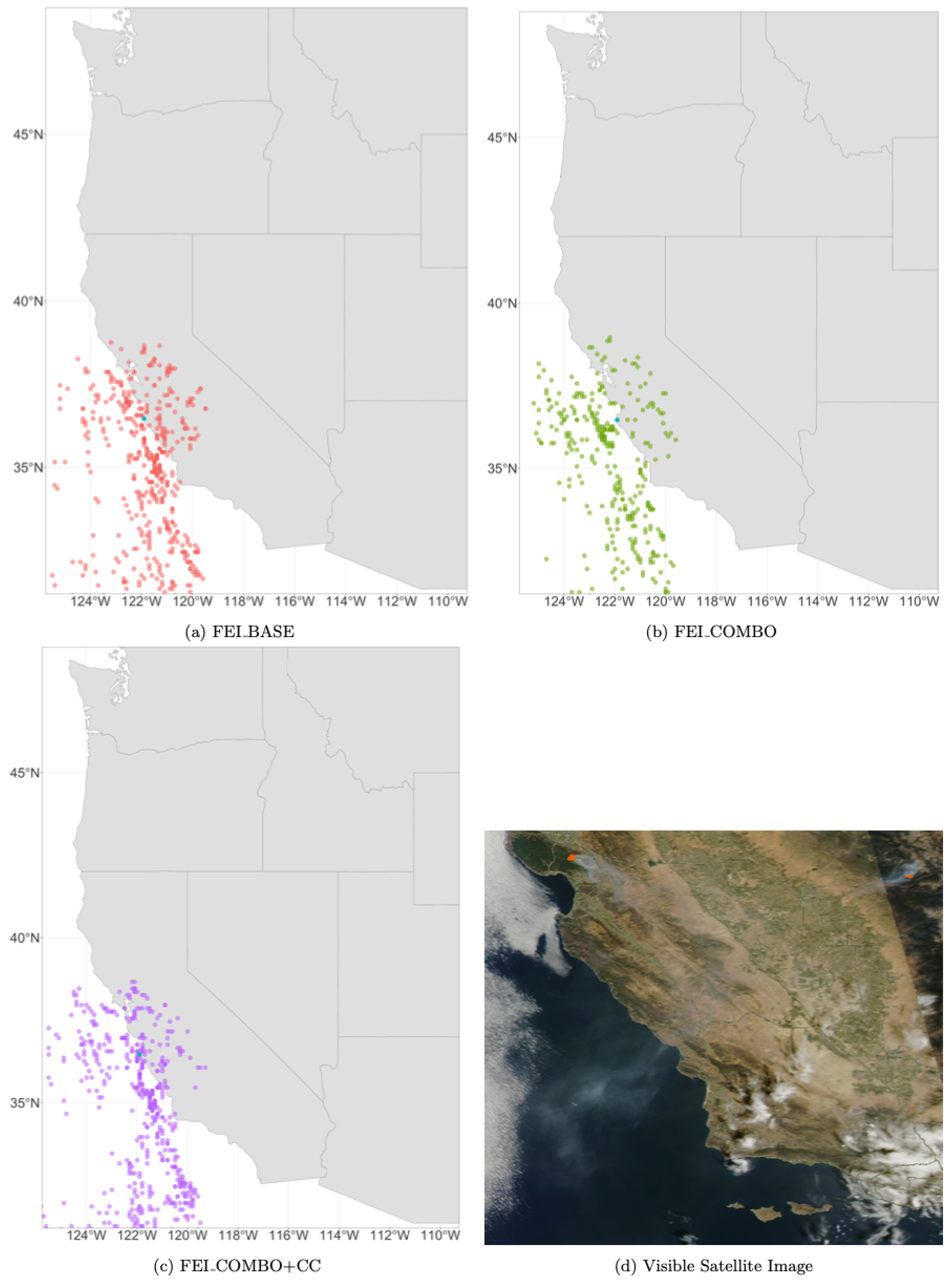
Comparing a HYSPLIT concentration map and visual imagery from NASA WorldView for a single day during the Carr Fire (4 August 2018) provides additional information (Figure 14). The visual image shows the Carr Fire plume being transported in two distinct plumes, one to the south and one to the west. The HYSPLIT concentration map captures this same trend. This can be indicative of vertical wind shear creating a broad area of smoke transport. This is supported by the HYSPLIT concentration map, which shows much wider locations of PM_2.5 concentration than are captured by the visual image. The differences between the FEIs are also more apparent than seen in the Rim Fire, suggesting that vertical wind shear may exacerbate the differences between the dispersion results from each FEI. The visible image also shows a very large fire south of the Carr Fire that is also producing a large smoke plume. This smoke plume does not show the two distinct plumes that the Carr Fire does, emphasizing the localized nature of boundary layer meteorology. The large fire may also be driving the winds in that fire area, providing a glimpse into the complicated nature of understanding the coupled fire–atmosphere interactions resulting from large fires. The HYSPLIT concentration map does not show the smoke plume from the large fire because the HYSPLIT concentration is specific to the Carr Fire. This can be useful in health studies, where different health effects can be assigned to the separate plumes instead of the mixed and transported plume.

4. Conclusions

This study shows that different fire emission inventories (FEIs) can cause large variation in estimated HYSPLIT PM_2.5 ambient concentrations. Comparisons with EPA monitoring data and satellite visible imagery highlights the differences between dispersion results in a variety of situations. FEI_COMBO+CC demonstrated modest but consistent improvements in correlation and bias across multiple sites and years compared to the other fire emission inventories. These improvements suggest that incorporating daily cloud cover gap-filling and refined burned area estimates can meaningfully enhance the temporal accuracy of emission inputs used in dispersion modeling, particularly for daily scale analyses.

Atmospheric dispersion models are useful to investigate smoke dispersion throughout the atmosphere. They are often used to estimate human exposure to fire smoke in health effect studies. For exposure modeling, discrepancies in the fire emissions information can result in missed human exposure and, thus, missed health effects. Quantifying the differences in HYSPLIT PM_2.5 concentrations that result from using different FEI information is an important step in understanding the uncertainties in the exposure modeling that informs human health effects studies.

While this work is an important step forward, there are numerous opportunities for future work. Correcting EPA PM_2.5 measurements to be fire-specific would allow for a more direct comparison between HYSPLIT and the EPA data, addressing some of the challenges of comparing the two data types [12]. A higher-resolution meteorology model (e.g., HRRR [41]) could reduce the uncertainties in the gridded model used to drive HYSPLIT, thus improving the dispersion modeling results. Using more complex atmospheric models (e.g., chemical transport models such as CMAQ and WRF-CHEM, or coupled fire–atmosphere systems like WRF-SFIRE), particularly for single-fire simulations, would allow for a deeper understanding of the complex chemical reactions in the atmosphere as smoke is transported downwind. The complexity of fire behavior and atmospheric transport means there are significant improvements that could be implemented for the fire–smoke–atmosphere modeling system related to developing improved FEIs, atmospheric models, plume rise models, and comparison datasets. Additionally, high-temporal-resolution geostationary satellite data from GOES-East and West (available from 2017 onward) could support more detailed smoke plume validation and tracking in future studies.

This study demonstrates the high sensitivity of HYSPLIT atmospheric dispersion model results to the choice of FEI, with modeled PM_2.5 concentrations varying by up to 200% annually depending on the input data. FEI_COMBO and FEI_COMBO+CC consistently increase the number of concentration locations and improve NMB compared to FEI_BASE, with FEI_COMBO+CC showing the lowest NMB across all study years. While RMSE, generally increases slightly with the additional FEI processing, especially in 2018, these results suggest improved emissions representation but highlight the need for continued refinement. Because dispersion modeling outputs are use in health effect studies and policy making, improving the accuracy of fire emission inputs remains essential. This work advances wildfire smoke exposure modeling, enabling more thorough health research and better-informed public health decisions.

References

1. Heilman, W.E.; Liu, Y.; Urbanski, S.; Kovalev, V.; Mickler, R. Wildland fire emissions, carbon, and climate: Plume rise, atmospheric transport, and chemistry processes. For. Ecol. Manag. 2014, 317, 70–79. [Google Scholar] [CrossRef]
2. Black, C.; Tesfaigzi, Y.; Bassein, J.A.; Miller, L.A. Wildfire smoke exposure and human health: Significant gaps in research for a growing public health issue. Environ. Toxicol. Pharmacol. 2017, 55, 186–195. [Google Scholar] [CrossRef]
3. Liu, J.C.; Mickley, L.J.; Sulprizio, M.P.; Dominici, F.; Yue, X.; Ebisu, K.; Anderson, G.B.; Khan, R.F.A.; Bravo, M.A.; Bell, M.L. Particulate air pollution from wildfires in the Western US under climate change. Clim. Change 2016, 138, 655–666. [Google Scholar] [CrossRef]
4. Reid, C.; Considine, E.; Watson, G.; Telesca, D.; Pfister, G.; Jerrett, M. Effect modification of the association between fine particulate air pollution during a wildfire event and respiratory health by area-level measures of socio-economic status, race/ethnicity, and smoking prevalence. Environ. Res. Health 2023, 1, 025005. [Google Scholar] [CrossRef]
5. Wilmot, T.Y.; Mallia, D.V.; Hallar, A.G.; Lin, J.C. Wildfire plumes in the Western US are reaching greater heights and injecting more aerosols aloft as wildfire activity intensifies. Sci. Rep. 2022, 12, 12400. [Google Scholar] [CrossRef] [PubMed]
6. Wiedinmyer, C.; Akagi, S.K.; Yokelson, R.J.; Emmons, L.K.; Al-Saadi, J.A.; Orlando, J.J.; Soja, A.J. The Fire INventory from NCAR (FINN): A high resolution global model to estimate the emissions from open burning. Geosci. Model Dev. 2011, 4, 625–641. [Google Scholar] [CrossRef]
7. Urbanski, S.P.; Reeves, M.C.; Corley, R.E.; Silverstein, R.P.; Hao, W.M. Contiguous United States wildland fire emission estimates during 2003–2015. Earth Syst. Sci. Data 2018, 10, 2241–2274. [Google Scholar] [CrossRef]
8. van der Werf, G.R.; Randerson, J.T.; Giglio, L.; van Leeuwen, T.T.; Chen, Y.; Rogers, B.M.; Mu, M.; van Marle, M.J.E.; Morton, D.C.; Collatz, G.J.; et al. Global fire emissions estimates during 1997–2016. Earth Syst. Sci. Data 2017, 9, 697–720. [Google Scholar] [CrossRef]
9. Mandel, J.; Kochanski, A.K.; Vejmelka, M.; Beezley, J.D. Data Assimilation of Satellite Fire Detection in Coupled Atmosphere-Fire Simulation by WRF-SFIRE. arXiv 2014, arXiv:1410.6948. [Google Scholar] [CrossRef]
10. Hawbaker, T.J.; Radeloff, V.C.; Syphard, A.D.; Zhu, Z.; Stewart, S.I. Detection rates of the MODIS active fire product in the United States. Remote Sens. Environ. 2008, 112, 2656–2664. [Google Scholar] [CrossRef]
11. Liu, T.; Mickley, L.J.; Marlier, M.E.; DeFries, R.S.; Khan, M.F.; Latif, M.T.; Karambelas, A. Diagnosing spatial biases and uncertainties in global fire emissions inventories: Indonesia as regional case study. Remote Sens. Environ. 2020, 237, 111557. [Google Scholar] [CrossRef]
12. Faulstich, S.; Strickland, M.; Holmes, H. Enhancing fire emissions inventories for acute health effects studies: Integrating high spatial and temporal resolution data. Int. J. Wildland Fire 2025, 34, WF24040. [Google Scholar] [CrossRef] [PubMed]
13. Sokolik, I.N.; Soja, A.J.; DeMott, P.J.; Winker, D. Progress and challenges in quantifying wildfire smoke emissions, their properties, transport, and atmospheric impacts. J. Geophys. Res. 2019, 124, 13005–13025. [Google Scholar] [CrossRef]
14. Miller, D.J.; Sun, K.; Zondlo, M.A.; Kanter, D.; Dubovik, O.; Welton, E.J.; Winker, D.M.; Ginoux, P. Assessing boreal forest fire smoke aerosol impacts on US air quality: A case study using multiple data sets. J. Geophys. Res. 2011, 116, D22209. [Google Scholar] [CrossRef]
15. Goodrick, S.L.; Achtemeier, G.L.; Larkin, N.K.; Liu, Y.; Strand, T.M. Modelling smoke transport from wildland fires: A review. Int. J. Wildland Fire 2012, 22, 83–94. [Google Scholar] [CrossRef]
16. Hosseini, S.; Urbanski, S.P.; Dixit, P.; Qi, L.; Burling, I.R.; Yokelson, R.J.; Johnson, T.J.; Shrivastava, M.; Jung, H.S.; Weise, D.R.; et al. Laboratory characterization of PM emissions from combustion of wildland biomass fuels: Particle emissions from biomass burning. J. Geophys. Res. D Atmos. 2013, 118, 9914–9929. [Google Scholar] [CrossRef]
17. Akagi, S.K.; Yokelson, R.J.; Wiedinmyer, C.; Alvarado, M.J.; Reid, J.S.; Karl, T.; Crounse, J.D.; Wennberg, P.O. Emission factors for open and domestic biomass burning for use in atmospheric models. Atmos. Chem. Phys. 2011, 11, 4039–4072. [Google Scholar] [CrossRef]
18. Stein, A.F.; Draxler, R.R.; Rolph, G.D.; Stunder, B.J.B.; Cohen, M.D.; Ngan, F. NOAA’s HYSPLIT atmospheric transport and dispersion modeling system. Bull. Am. Meteorol. Soc. 2015, 96, 2059–2077. [Google Scholar] [CrossRef]
19. Rolph, G.D.; Draxler, R.R.; Stein, A.F.; Taylor, A.; Ruminski, M.G.; Kondragunta, S.; Zeng, J.; Huang, H.C.; Manikin, G.; McQueen, J.T.; et al. Description and Verification of the NOAA Smoke Forecasting System: The 2007 Fire Season. Weather Forecast. 2009, 24, 361–378. [Google Scholar] [CrossRef]
20. Tinling, M. Emergency Department Diagnoses In Eastern North Carolina Associated with Smoke Exposure from the 2011 Pains Bay Wildfire. Ph.D. Thesis, University of North Carolina at Chapel Hill, Chapel Hill, NC, USA, 2012. [Google Scholar] [CrossRef]
21. Thelen, B.; French, N.H.F.; Koziol, B.W.; Billmire, M.; Owen, R.C.; Johnson, J.; Ginsberg, M.; Loboda, T.; Wu, S. Modeling acute respiratory illness during the 2007 San Diego wildland fires using a coupled emissions-transport system and generalized additive modeling. Environ. Health 2013, 12, 94. [Google Scholar] [CrossRef] [PubMed]
22. Uda, S.K.; Hein, L.; Atmoko, D. Assessing the health impacts of peatland fires: A case study for Central Kalimantan, Indonesia. Environ. Sci. Pollut. Res. 2019, 26, 31315–31327. [Google Scholar] [CrossRef] [PubMed]
23. Johnson, M.M.; Garcia-Menendez, F. Uncertainty in Health Impact Assessments of Smoke From a Wildfire Event. GeoHealth 2022, 6, e2021GH000526. [Google Scholar] [CrossRef] [PubMed]
24. Ngan, F.; Loughner, C.P.; Stein, A. The evaluation of mixing methods in HYSPLIT using measurements from controlled tracer experiments. Atmos. Environ. 2019, 219, 117043. [Google Scholar] [CrossRef]
25. French, N.H.F.; McKenzie, D.; Erickson, T.; Koziol, B.; Billmire, M.; Endsley, K.A.; Yager Scheinerman, N.K.; Jenkins, L.; Miller, M.E.; Ottmar, R.; et al. Modeling Regional-Scale Wildland Fire Emissions with the Wildland Fire Emissions Information System. Earth Interact. 2014, 18, 1–26. [Google Scholar] [CrossRef]
26. Giglio, L.; Boschetti, L.; Roy, D.P.; Humber, M.L.; Justice, C.O. The Collection 6 MODIS burned area mapping algorithm and product. Remote Sens. Environ. 2018, 217, 72–85. [Google Scholar] [CrossRef] [PubMed]
27. Eidenshink, J.; Schwind, B.; Brewer, K.; Zhu, Z.L.; Quayle, B.; Howard, S. A Project for Monitoring Trends in Burn Severity. Fire Ecol. 2007, 3, 3–21. [Google Scholar] [CrossRef]
28. CalFire. Rim Fire. 2013. Available online: https://www.fire.ca.gov/incidents/2013/8/17/rim-fire/ (accessed on 30 January 2021).
29. CalFire. Soberanes Fire. 2022. Available online: https://www.fire.ca.gov/incidents/2016/7/22/soberanes-fire (accessed on 7 March 2025).
30. CalFire. Carr Fire. 2022. Available online: https://www.fire.ca.gov/incidents/2018/7/23/carr-fire (accessed on 7 March 2025).
31. Briggs, G.A. Plume Rise: A Critical Survey; Technical Report; US. Atomic Energy Commission, Division of Technical Information: Oak Ridge, TN, USA, 1969. [CrossRef]
32. National Centers for Environmental Prediction; National Weather Service; NOAA; U.S. Department of Commerce. NCEP North American Mesoscale (NAM) 12 km Analysis; National Centers for Environmental Prediction: College Park, MD, USA, 2015. [CrossRef]
33. NOAA. Index of /Data/Archives/nam12. 2007. Available online: https://www.ready.noaa.gov/data/archives/nam12/ (accessed on 7 March 2025).
34. EPA. EPA AirData Website File Download Page. 2015. Available online: https://aqs.epa.gov/aqsweb/airdata/download_files.html (accessed on 7 March 2025).
35. NASA. NASA Worldview. 2021. Available online: https://worldview.earthdata.nasa.gov (accessed on 7 March 2025).
36. Jacobson, M.Z. Short-term effects of agriculture on air pollution and climate in California. J. Geophys. Res. Atmos. 2008, 113, D23101. [Google Scholar] [CrossRef]
37. Loría-Salazar, S.M.; Sayer, A.M.; Barnes, J.; Huang, J.; Flynn, C.; Lareau, N.; Lee, J.; Lyapustin, A.; Redemann, J.; Welton, E.J.; et al. Evaluation of novel NASA moderate resolution imaging spectroradiometer and visible infrared imaging radiometer suite aerosol products and assessment of smoke height boundary layer ratio during extreme smoke events in the western USA. J. Geophys. Res. 2021, 126, e2020JD034180. [Google Scholar] [CrossRef]
38. Wang, D.; Guan, D.; Zhu, S.; Kinnon, M.M.; Geng, G.; Zhang, Q.; Zheng, H.; Lei, T.; Shao, S.; Gong, P.; et al. Economic footprint of California wildfires in 2018. Nat. Sustain. 2020, 4, 252–260. [Google Scholar] [CrossRef]
39. Averett, N. Smoke Signals: Teasing Out Adverse Health Effects of Wildfire Emissions. Environ. Health Perspect. 2016, 124, A166. [Google Scholar] [CrossRef]
40. Grant, E.; Runkle, J.D. Long-term health effects of wildfire exposure: A scoping review. J. Clim. Change Health 2022, 6, 100110. [Google Scholar] [CrossRef]
41. Dowell, D.C.; Alexander, C.R.; James, E.P.; Weygandt, S.S.; Benjamin, S.G.; Manikin, G.S.; Blake, B.T.; Brown, J.M.; Olson, J.B.; Hu, M.; et al. The High-Resolution Rapid Refresh (HRRR): An hourly updating convection-allowing forecast model. Part I: Motivation and system description. Weather Forecast. 2022, 37, 1371–1395. [Google Scholar] [CrossRef]
Figure 1. A map of the spatial domain and the EPA monitor locations used in this study. The red box represents the spatial domain. Reno and Sparks are geographically close and appear overlapping at this scale.
Fire 08 00331 g001
Figure 2. Correlation between 2013 HYSPLIT modeled smoke PM2.5 concentration using each FEI and the EPA measured PM2.5 concentration. Note: EPA measurements are not wildfire smoke specific and includes PM2.5 from all sources.
Fire 08 00331 g002
Figure 3. Correlation between 2016 HYSPLIT modeled PM2.5 concentration using each FEI and the EPA measured PM2.5 concentration. Note: EPA measurements are not wildfire smoke specific and includes PM2.5 from all sources.
Fire 08 00331 g003
Figure 4. Correlation between 2018 HYSPLIT modeled smoke PM2.5 concentration using each FEI and the EPA measured PM2.5 concentration. Note: EPA measurements are not wildfire smoke specific and includes PM2.5 from all sources.
Fire 08 00331 g004
Figure 5. The 2013 Rim Fire daily PM2.5 concentrations in Reno, NV, from HYSPLIT using all three FEIs.
Fire 08 00331 g005
Figure 6. Daily HYSPLIT PM2.5 ambient smoke concentration grid points at 10 m for each of the three FEIs (represented in red, green, and purple) on 24 August 2013, during the Rim Fire and a visual satellite image of the Rim fire on 24 August 2013, from NASA WorldView (MODIS Terra). The Rim Fire is circled in red. The smaller orange dots represent thermal anomalies captured by MODIS Terra and Aqua, showing the location of the fire.
Fire 08 00331 g006
Figure 7. The 2016 Soberanes Fire daily PM2.5 concentrations in Reno, NV, from HYSPLIT using all three FEIs.
Fire 08 00331 g007
Figure 8. Daily HYSPLIT PM2.5 ambient smoke concentration grid points at 10 m for each of the three FEIs (represented in red, green, and purple) on 30 August 2016, during the Soberanes Fire and a visual satellite image of the Soberanes fire on 30 August 2016, from NASA WorldView (MODIS Terra). The Soberanes Fire is circled in red. The smaller orange dots represent thermal anomalies captured by MODIS Terra and Aqua, showing the location of the fire.
Fire 08 00331 g008
Figure 9. Daily HYSPLIT PM2.5 ambient smoke concentration grid points for each of the three FEIs (represented in red, green, and purple) on 26 September 2016, during the Soberanes Fire and a visual satellite image of the Soberanes Fire on 26 September 2016, from NASA WorldView (MODIS Aqua). The Soberanes Fire is circled in red. The visible satellite image shows a faint smoke plume. The smaller orange dots represent thermal anomalies captured by MODIS Terra and Aqua, showing the location of the fire.
Fire 08 00331 g009
Figure 10. HYSPLIT PM2.5 ambient concentration locations for each of the three FEIs (represented in red, green, and purple) on 27 September 2016, during the Soberanes Fire and a visual satellite image of the Soberanes Fire on 27 September 2016, from NASA WorldView. The Sobeanes fire is not captured in the visible imagery of this day.
Fire 08 00331 g010
Figure 11. Daily HYSPLIT PM2.5 ambient smoke concentration grid points for each of the three FEIs on (represented in red, green, and purple) 28 September 2016, during the Soberanes Fire and a visual satellite image of the Soberanes Fire on 28 September 2016, from NASA WorldView (MODIS Aqua). Thermal anomalies from the Soberanes fire are not captured by MODIS Terra and Aqua on this day.
Fire 08 00331 g011
Figure 12. Daily HYSPLIT PM2.5 ambient smoke concentration grid points for each of the three FEIs on (represented in red, green, and purple) 29 September 2016, during the Soberanes Fire and a visual satellite image of the Soberanes Fire on 29 September 2016, from NASA WorldView (MODIS Aqua). The Soberanes Fire is circled in red. The smaller orange dots represent thermal anomalies captured by MODIS Terra and Aqua, showing the location of the fire.
Fire 08 00331 g012
Figure 13. The 2018 Carr Fire daily PM2.5 concentrations in Reno, NV, from HYSPLIT using all three FEIs.
Fire 08 00331 g013
Figure 14. Daily HYSPLIT PM2.5 ambient smoke concentration grid points for each of the three FEIs on 4 August 2018, during the Carr Fire and a visual satellite image of the Carr Fire on 4 August 2016, from NASA WorldView (MODIS Aqua). The Carr Fire is circled in red. The smaller orange dots represent thermal anomalies captured by MODIS Terra and Aqua, showing the location of the fire. This is an example of a day with numerous smoke plumes that mix in the atmosphere.
Fire 08 00331 g014