Effective Comparison of Thermo-Mechanical Characteristics of Self-Compacting Concretes Through Machine Learning-Based Predictions ^†

Abstract

This present study proposes different machine learning-based predictors for the assessment of the residual compressive strength of Self-Compacting Concrete (SCC) subjected to high temperatures. The investigation is based on several literature algorithmic approaches based on Artificial Neural Networks with distinct training algorithms (Bayesian Regularization, Levenberg–Marquardt, Scaled Conjugate Gradient, and Resilient Backpropagation), Support Vector Regression, and Random Forest methods. A training database of 150 experimental data points is derived from a careful literature review, incorporating temperature (20–800 °C), geometric ratio (height/diameter), and corresponding compressive strength values. A statistical analysis revealed complex non-linear relationships between variables, with strong negative correlation between temperature and strength and heteroscedastic data distribution, justifying the selection of advanced machine learning techniques. Feature engineering improved model performance through the incorporation of quadratic terms, interaction variables, and cyclic transformations. The Resilient Backpropagation algorithm demonstrated superior performance with the lowest prediction errors, followed by Bayesian Regularization. Support Vector Regression achieved competitive accuracy despite its simpler architecture. Experimental validation using specimens tested up to 800 °C showed a good reliability of the developed systems, with prediction errors ranging from 0.33% to 23.35% across different temperature ranges.

1. Introduction

The increasing frequency and severity of fire events worldwide poses significant challenges to urban infrastructure and building safety. Climate change and urbanization have intensified fire risks in both rural and urban environments, making the assessment of structural resilience under thermal loading an engineering priority [1,2]. Post-fire structural evaluation requires an accurate understanding of material behavior degradation at elevated temperatures, particularly for modern construction materials with complex compositions [3,4].

Reinforced concrete structures face specific issues during fire exposure, as thermal effects can cause microscopic alterations in constituent materials that compromise overall structural integrity [5]. The combination of high temperatures and prolonged exposure introduces complex degradation mechanisms that affect both immediate fire resistance and post-fire residual capacity [6,7]. Self-Compacting Concrete (SCC), increasingly used in modern buildings due to its good workability and mechanical properties, presents additional challenges due to its modified composition and behavior under thermal loading [8]. The evolution of SCC compressive strength with temperature follows non-linear relationships dependent on geometric and mechanical parameters, requiring comprehensive experimental characterization that is often time-consuming and resource intensive [9]. Traditional laboratory testing approaches could be insufficient for the rapid assessment needs of post-fire structural evaluation, where timely decisions regarding structural safety and rehabilitation strategies are critical [10].

Artificial Neural Networks (ANNs) offer promising solutions for addressing these challenges by providing rapid, accurate predictions of material behavior based on limited input parameters. Neural network-based approaches can significantly reduce the time and resources required for post-fire assessment while maintaining the prediction accuracy necessary for engineering decision-making. Such predictive models are particularly valuable for evaluating exceptional loading scenarios where extensive experimental databases may not be readily available. Tools that leverage artificial intelligence facilitate the automatic gathering and examination of data relevant to design, covering aspects such as energy measures, material characteristics, and environmental features [11,12,13]. In the process of design stages, advanced algorithms could assess different options via generative design, analyze resource-efficient solutions, and develop execution plans that minimize risk [14,15]. Furthermore, the use of smart systems is extremely important for the monitoring of the health of relevant infrastructure projects (such as bridges, pipelines and dams, etc.). In fact, the installation of smart sensors allows the implementation of continuous monitoring strategies and vulnerability assessments of structures to maintain high levels of efficiency and safety over time [16,17].

The use of neural network-based models also makes it possible to streamline and reduce all the processes involved in carrying out laboratory or in situ tests [18,19]. This is relevant during the design phase, where it is necessary to know the mechanical properties of materials in detail, as well as during the intervention phase, (e.g., after earthquakes or fires), where it is of extreme interest to know the mechanical behavior of damaged materials. In particular, the use of AI systems would reduce the processing time and, in some cases, even the number of physical tests required. In the case of surveys in risky situations (ex-post), it could also ensure the safety of operators by highlighting risks and critical issues that might not be considered with the usual computational systems.

A significant challenge in thermal testing of concrete is the lack of standardized protocols defining test temperatures, exposure durations, and heating rates. Current practice typically relies on RILEM guidelines or fire resistance code criteria, but these provide limited guidance for comprehensive material characterization [20,21]. The trained neural networks developed in this study address this limitation by enabling virtually unlimited thermal simulations, allowing reconstruction of complete mechanical property evolution across the temperature spectrum from sparse experimental testing.

Several examples of the application of different types of machine learning networks and algorithms to the field of civil engineering can be found in the literature [22,23,24]. The cases are numerous and range from hydraulic [25,26,27,28] to structural engineering [29,30,31,32,33,34]. Particularly in the field of construction, several models have been developed to assess the health of a structure, both in the static and dynamic domains [35,36,37]. Other models have been developed to parameterize the design phase of innovative structures and to simplify their calculation [38,39,40]. In construction, concrete certification requires test specimens with a minimum 28-day curing period plus bureaucratic processing time. This time-consuming process is susceptible to human error and requires significant resources. Machine learning models can address these challenges by predicting concrete compressive strength through digital simulations, significantly reducing both physical testing requirements and experimental timeframes. However, developing such models requires thorough understanding of raw material relationships and how each component influences results [41,42]. While it is possible to derive mathematical equations and conduct simulations based on these relationships, we cannot assume that these relationships will translate identically to real-world conditions. Fortunately, extensive testing has been conducted over time, providing substantial real-world data that can be utilized for predictive modeling [43].

From a restoration perspective, having the ability to estimate the degree of damage that a specific structural element may have sustained would enable the safe planning and organization of investigation campaigns for degraded buildings. In this context, we will focus specifically on fire damage [44,45,46,47,48,49]. Moreover, this capability would allow for more precise and accurate optimization of restoration and consolidation intervention designs.

Ensemble learning represents an advanced methodology that improves predictive model performance by combining multiple neural networks or learning algorithms [50,51,52]. This strategy is based on the idea that aggregating predictions from diverse models can lead to more accurate and generalizable results. This approach leverages the “wisdom of the crowd” concept, where aggregated predictions from diverse models yield more accurate and generalizable results [53].

Beginning in the 1980s, the construction industry has set a higher priority on the optimization of material performance, which has resulted in the development of innovative concrete types, such as Self-Compacting Concrete (SCC). Self-Compacting Concrete shows good efficiency in scenarios where the vibration of formwork presents challenges or where there is a risk of segregation. Nonetheless, uncertainties remain regarding its service behavior [54,55,56,57], particularly in terms of evolution of compressive strength with temperature, which exhibits a non-linear relationship governed by geometric and mechanical parameters [9,58].

The investigation of residual mechanical strength after damaging events such as fires often requires extensive and expensive tests. This study proposes a supplementary approach that uses neural algorithms to improve the investigation of the residual strength of SCC after exposure to high temperatures. The numerical models in question should be seen as a complement to experimental tests. They provide expected value ranges that may assist in establishing test protocols and reducing the number of tests, resulting in cuts in both time and cost. Predictive models play a useful role in preventing dangerous in situ tests on fire-damaged structures. The ability to avoid the use of destructive testing is also important for historic buildings where it is difficult to operate, or for structures that are in extreme conditions (e.g., oil rig foundations) from which it would be extremely difficult to take samples.

AI models offer significant computational advantages over classical finite element models. While detailed structural modeling requires extensive knowledge of thermal and mechanical material behavior, our proposed methodology obtains reliable results within minutes. However, both methodologies can be combined for more refined analyses. This study advances the state-of-the-art by providing the first comprehensive comparison of several neural networks specifically designed for predicting SCC thermal behavior, incorporating advanced feature engineering with interaction terms and cyclic transformations. This research validates predictions across the temperature spectrum of ordinary building fires (20–800 °C) using controlled experimental data, providing evidence-based algorithm selection criteria and uncertainty bounds for post-fire structural assessment. Additionally, this work addresses a gap in testing standards and normative guidance for thermal assessment of modern concrete formulations.

In the last few years, several researchers have investigated the possibility of using ML to determine the compressive strength of concrete. Various algorithms have been proposed to predict the compressive strength of concrete based on conventional regression analysis and statistical models [59,60,61,62,63,64,65,66,67,68]. It is noteworthy that in similar studies, neural networks have been shown to outperform regression methods in predicting the compressive strength of concrete [43,69,70,71,72,73,74,75]. With enough input data, ML models can be trained to predict the compressive strength of concrete. Yeh [76] used an artificial neural network with an input layer of eight units, a hidden layer of eight units, and an output layer of one unit to predict the compressive strength of concrete. A validation R²-value of 0.9418 was obtained, proving the high-precision prediction capability of the model. Khademi et al. [77] employed multiple linear regression (MLR) and an adaptive neuro-fuzzy inference system to estimate the compressive strength of concrete; similarly, Ashrafian et al. [78] predicted the compressive strength and ultrasonic pulse velocity of fiber-reinforced concrete using heuristic regression methods. Using a Random Forest algorithm, Mai et al. [79] were able to predict the compressive strength of concrete containing ground granulated blast furnace slag with a high degree of accuracy. Feng et al. [74] used a learner-based adaptive boosting algorithm to predict the compressive strength of concrete with a low error, achieving coefficient of determination values as high as 0.952. Li et al. [80] used MLR and an adaptive neuro-fuzzy inference system to estimate the rock tensile strength obtained from the Brazilian tensile strength test. Their results showed that the adaptive neuro-fuzzy inference system predicted compressive strength values closest to the actual test values. Asteris et al. [81] used artificial neural network models to predict the compressive strength of concrete, incorporating metakaolin, which is widely used to reduce the cement requirement in concrete. Their model provided remarkable accuracy in predicting compressive strength based on six inputs. Ali, Muayad, Mohammed, and Asteris [82] predicted the compressive strength of concrete with different nano-silica (nano-particle) contents using six models: linear regression, MLR, non-linear regression, pure quadratic, interaction, and full quadratic. They concluded that the full quadratic model provided better accuracy in predicting compressive strength, with an R² of 0.96.

This research aims to identify and validate a robust machine learning framework designed to predict the residual compressive strength of Self-Compacting Concrete (SCC) when exposed to elevated temperatures. The analysis focuses on the ability of different machine learning methodologies to effectively capture the intricate relationships among temperature exposure, specimen geometry, and residual strength. The proposed approach involves the development of predictive models together with an exhaustive validation process that compares these models with experimental data.

This paper is organized as follows: In Section 2, a review of the artificial neural network architectures is presented, covering the mathematical concepts behind Bayesian Regularization, Levenberg–Marquardt, Scaled Conjugate Gradient, Resilient Backpropagation, Support Vector Regression, and Random Forest algorithms. Section 3 describes the assembly of the training database and provides a statistical analysis of the collected data, which informed modeling decisions. Section 4 presents the numerical methodology, including data preprocessing, feature engineering, and the optimization strategies used for each algorithm. Section 5 provides details of the experimental campaign performed to validate the models. Section 6 discusses the results obtained, comparing the performance of the different algorithms while examining their predictive abilities across a range of temperature deviations and geometric configurations. In conclusion, Section 7 summarizes the principal findings and addresses their relevance for practical applications in the context of structural fire engineering.

2. Materials and Methods

2.1. ANN Models

The architecture of a standard Artificial Neural Network (ANN) includes some input nodes, one or more hidden layers, each with k nodes, and several output nodes. The input layer accepts initial data such as geometrical configurations, material properties, and other physical parameters defined by the user. The hidden layers process this data through computational operations, and the output layer delivers the final calculated values. An ANN establishes connections between every neuron of one layer to every neuron of the subsequent layer. Only after undergoing a training phase with a designated dataset comprising input–output pairs can the ANN be utilized for prediction tasks. The prevalent method for training ANNs is the supervised learning algorithm known as back-propagation. This algorithm encompasses a minimization procedure that unfolds in three stages [83]. Initially, the input data x_k progresses forward through the network to produce the output y_i, corresponding to the nodes of the output layer in an ANN with a singular hidden layer. The operation for the i-th node output is given by Equation (1):

$$y_i=\mathrm{g}\left[w_{ij}g\left(v_{jk}{x}_k+{\theta }_{vj}\right)+{\theta }_{wi}\right]$$

(1)

where y_i represents the output from the i-th node in the output layer, x_k is the input to the k-th node in the input layer, $w_{ij}$ is the weight connecting the hidden layer nodes to the output layer nodes, $v_{jk}$ is the weight connecting the input layer nodes to the hidden layer nodes, ${\theta }_{vj}$ and ${\theta }_{wi}$ are the bias terms, and g is a transfer function. The indices k, j, and i refers to the counts of nodes in the input, hidden, and output layers, respectively. The ANN performance is monitored through an error function that calculates the error between the expected and the actual output values for each node in the output layer. The training involves a feedback loop, which constantly adjusts the weights, $W_{ij}$ and $V_{jk}$, and the biases, ${\theta }_{vj}$ and ${\theta }_{wi}$, to minimize this error and enhance performance.

The selection of the neural networks to be tested was based on the necessity to examine algorithms that exhibited a balance between predictive capacity, robustness, and speed of convergence. In particular, the problem under analysis requires an approach that is sensitive to the non-linear complexity of the data, while ensuring the capacity for generalization even on relatively small datasets. The four selected network types represent well-established and widely used approaches, each with distinctive characteristics:

• Bayesian Regularization is an optimal method for addressing the issue of overfitting, particularly when the available data is limited and highly noisy.
• The Levenberg–Marquardt method is renowned for its rapid convergence, rendering it an optimal choice for small to moderate datasets.
• Scaled Conjugate Gradient (SCG) is an optimized variant of gradient methods, designed to ensure stable convergence even in the presence of complex parametric spaces.
• Resilient Backpropagation (RProp) is a method that focuses on the independent updating of weights, thereby ensuring robustness against gradient-scaling problems.

The four types represent a combination of gradient-based strategies, regularized techniques, and scalable approaches, offering comprehensive coverage of the main methodologies applicable to complex regression problems.

2.1.1. Bayesian Regression Model

In this research, a Bayesian regression algorithm was used to train the neural networks handling all output parameters [84,85]. The scope was the prediction of the ultimate compressive strength of Self-Compacting Concrete as the temperature changes.

Regularization is integrated into the objective function through the introduction of an additional term that penalizes the complexity of the model. The overall objective function can be expressed as in Equation (2):

$$F=E_D+\lambda E_W$$

(2)

where the error term on the training data, E_D, is typically expressed as the sum of squares of errors, $E_D={\sum }_i{(y_i-\widehat{y_i})}^2$. The sum of squares of the network weights, $E_W={\sum }_j{w}_j^2$, is also a key factor. Finally, λ is a parameter that controls the balance between minimizing the error on the data and penalizing the complexity of the model.

This method is based on Bayesian probability principles, where network weights are treated as random variables with prior distributions. During training, the posterior distribution of weights is optimized by combining data-derived information (likelihood) with prior knowledge. The regularization effect results directly from the prior distribution, which favors solutions with smaller weights. In computational terms, Bayesian Regularization is implemented through the dynamic adaptation of the parameter λ. This parameter is updated during optimization to automatically balance the two terms of the objective function, obviating the need for manual tuning. This iterative process is integrated into the optimization algorithm, which is typically a variant of the Gauss–Newton method.

In the context of MATLAB neural networks, the Bayesian Regularization method is implemented using the trainbr function, which is used to train a Bayesian Regularization model [86]. The algorithm updates the weights and biases of the network by minimizing the regularized objective function. The algorithm requires the definition of a network comprising one or more hidden layers and the application of global regularization. The iterative calculation entails the evaluation and updating of the gradient of the objective function with respect to the network weights, thereby enabling the dynamic adaptation of the parameters to optimize the model generalizability.

Bayesian Regularization is particularly well-suited to contexts where datasets are limited in size, or the signal-to-noise ratio is low. The capacity to automatically address regularization and mitigate the likelihood of overfitting renders it an optimal instrument for intricate regression challenges, guaranteeing resilience and equilibrium between model accuracy and simplicity.

2.1.2. Levenberg–Marquardt Model

Levenberg–Marquardt (LM) is an iterative algorithm utilized for the optimization of Artificial Neural Networks, exhibiting good efficacy in the context of non-linear regression problems. This method combines the advantages of the descending gradient and the Gauss–Newton approach through a dynamic adaptation of the update step, thereby ensuring stability and efficiency. The NN weights are updated as in Equation (3):

$$\mathsf{\Delta }w=-{\left(J^{T}J+\mu I\right)}^{-1}{J}^{T}e$$

(3)

where J is the Jacobian matrix of residuals e; J^TJ represents an estimate of the Hexian approximation; μ is a damping parameter controlling the transition between the Gauss–Newton method (μ→0) and the descending gradient (μ→∞); I is the identity matrix; and e represents the residuals, i.e., the difference between observed and predicted values.

The LM method adaptively adjusts the μ value during training. When an update step reduces the error, μ is decreased, aligning the behavior with the Gauss–Newton method and accelerating convergence. Conversely, when the error increases, μ is increased, causing the method to behave like gradient descent.

This flexibility enables effective traversal of complex parameter spaces, making the method particularly suitable for neural networks with moderate parameter counts. The LM method’s primary advantage is its rapid convergence compared to other optimization algorithms, especially when the objective function is well-approximated by a local quadratic relationship. However, the algorithm is computationally intensive, requiring storage and inversion of the J^TJ matrix, whose computational cost increases rapidly with network weight count. This limitation makes the method less suitable for networks with substantial parameter numbers.

The Levenberg–Marquardt method was implemented using the trainlm function from the MATLAB Neural Network Toolbox [86]. This function fully exploits LM method features through an iterative optimization process that combines flexibility with rapid convergence.

2.1.3. Scaled Conjugate Gradient (SCG) Model

The Scaled Conjugate Gradient (SCG) algorithm represents a refinement of optimization techniques based on conjugate gradient methods, specifically designed for training neural networks. The SCG method is distinguished by its reliance on a line search-free approach, which markedly diminishes the computational burden relative to conventional techniques. The SCG method is founded upon the minimization of an objective function, designated as E, which represents the training error. This is achieved through the iterative updating of the network weights. The process of updating the weights is defined as in Equation (4):

$$\mathsf{\Delta }{w}_k={\lambda }_k{d}_k$$

(4)

where d_k is the direction of the conjugate gradient calculated iteratively and λ_k is a scaling parameter that is automatically determined at each step, balancing the trade-off between speed of convergence and stability.

Unlike classical conjugate gradient methods that require searching for optimal step length along the d_k direction, the SCG method uses second derivative approximation (Hessian) to determine λ_k. This approach eliminates the need for explicit Hessian matrix computation, reducing both training time and computational complexity.

The SCG method was implemented using the trainscg function from the MATLAB Neural Network Toolbox [86]. This function combines computational efficiency with robustness, making it suitable for networks with large parameter counts or extensive datasets. During training, trainscg iteratively computes d_k directions using local target function information, ensuring stable updates and reducing local minima convergence risk. A key feature of trainscg is automatic scaling parameter management, allowing dynamic adaptation to problem characteristics. This makes the method particularly effective for problems with complex error function topology or poorly defined gradients.

2.1.4. Resilient Backpropagation (RProp) Model

The Resilient Backpropagation (RProp) algorithm represents a sophisticated optimization technique for neural network training, which directly addresses the issues associated with gradient propagation [87]. RProp has been designed to overcome the limitations of small or large magnitude gradients and operates by changing weights in accordance with the direction of the gradient, while ignoring its amplitude. This approach is intended to ensure a stable and effective update of weights, regardless of the gradient scale.

The Resilient Backpropagation algorithm is founded upon the concept of modifying the weights w_ij through the application of an adaptive increment Δw_ij, which is calculated in accordance with Equation (5):

$${∆w}_{ij}^{(t+1)}=\left\{\begin{array}{c}-{\eta }_{ij} if {{\displaystyle \frac{\partial E}{\partial w_{ij}}}}^{\left(t\right)}·{{\displaystyle \frac{\partial E}{\partial w_{ij}}}}^{(t-1)}>0\\ +{\eta }_{ij} if {{\displaystyle \frac{\partial E}{\partial w_{ij}}}}^{\left(t\right)}·{{\displaystyle \frac{\partial E}{\partial w_{ij}}}}^{(t-1)}<0\\ 0 otherwise\end{array}\right.$$

(5)

where ${\displaystyle \frac{\partial E}{\partial w_{ij}}}$ is the error gradient relative to weight w_ij and ${\eta }_{ij}$ is the adaptive value that determines the amount of the update for each weight.

Resilient Backpropagation’s main advantage lies in decoupling update direction from gradient magnitude. This mechanism resolves issues arising from gradients with disparate scales or those dominated by noisy numerical components. The method avoids direct gradient amplitude utilization, updating weights with steps independent of gradient scale.

Additionally, the local adaptability of η_ij provides notable advantages by allowing individual weight adjustments during optimization. This approach offers greater flexibility and robustness compared to global learning step methods such as stochastic gradient descent.

Resilient Backpropagation was implemented using the trainrp function, available in MATLAB for neural networks [86]. The trainrp method incorporates fundamental Resilient Backpropagation principles, iteratively updating network weights until satisfactory convergence or maximum iteration count is reached. Resilient Backpropagation proves particularly effective when loss function gradients exhibit variable oscillations or scales. It provides a compromise between robustness and convergence speed, making it a preferred method for single-layer and multi-layer neural networks.

2.2. Support Vector Regression (SVR) Model

Support Vector Regression (SVR) represents an extension of the Support Vector Machines (SVM) methodology, specifically designed for regression problems. The fundamental principle of SVR is to achieve a balance between model complexity and prediction accuracy by defining a function that minimizes deviations from target values within a tolerable range ε. This approach allows for the development of a robust model that is capable of effective generalization even in the presence of noisy or complex data.

The objective function of the SVR is constructed by combining two terms: the minimization of the standard deviation of the model weights β, which ensures simplicity of the function, and a penalty proportional to the sum of the deviations ξ and ξ^*, representing violations of the ε margin. Formally, the optimization problem is expressed as in Equation (6):

$$\begin{array}{c}min\\ \beta ,b,\xi ,{\xi }^{*}\end{array}{\displaystyle \frac{1}{2}}{‖\beta ‖}^2+C\sum _{i=1}^n\left({\xi }_i+{\xi }_i^{*}\right)$$

(6)

subject to the following constraints, reported in Equation (7):

$$\begin{gathered} y_i-\left({\beta }^T{x}_i+b\right)\le ϵ+{\xi }_i, \\ \left({\beta }^T{x}_i+b\right)-y_i\le ϵ+{\xi }_i^{*}, \\ {\xi }_i,{\xi }_i^{*}\ge 0,\hspace{1em}i=1, \dots , n. \end{gathered}$$

(7)

In this formulation, C represents a setting parameter that serves to balance the trade-off between the tolerable error margin and the model’s capacity to adapt to the training data.

A principal component of the SVR is the utilization of kernel functions, which facilitate the mapping of data into a high-dimensional space, thereby enabling the modeling of non-linear relationships. The kernel is used to compute the implicit scalar product in the transformed space, which defines the similarity between pairs of points.

In this present study, three distinct kernel types were considered for the construction of Support Vector Regression (SVR) models: linear, polynomial, and radial basic (RBF). This was achieved through the utilization of the fitrsvm function within the MATLAB R2020b software [86]. Each kernel was selected and optimized in accordance with its specific characteristics, thereby ensuring an optimal compromise between flexibility and generalization capabilities.

The selection and optimization of the kernel parameters were conducted through a layered cross-validation process, ensuring a robust evaluation of the model performance and the identification of the optimal configuration for each kernel type.

2.3. Random Forest Model

Random Forest is a supervised learning method based on the construction of decision-making tree ensembles. The fundamental premise is to integrate the forecasts from numerous decision trees, each constructed on a randomly selected subset of the data set, with the objective of minimizing variance and enhancing predictive efficacy. Each tree is trained on a bootstrap sample of the dataset, and a random subset of predictors is considered at each split, thereby introducing diversity among the trees.

In case of regression, given a set of trees T₁, T₂, … T_k, the final prediction is given by Equation (8):

$$\widehat{y}={\displaystyle \frac{1}{k}}\sum _{i=1}^k{T}_i\left(x\right)$$

(8)

where $T_i\left(x\right)$ is the prediction of the i-th tree for an x observation.

A distinctive feature of Random Forest is the random selection of variables during node construction. This procedure limits the influence of dominant variables, reducing overfitting risk and promoting tree diversity. During node construction, the algorithm considers a random subset of predictors rather than all available variables, improving model generalization. The optimal predictor for each node is selected by maximizing an impurity criterion, such as the Gini index for classification or mean square error reduction for regression. Bootstrap sampling creates Out-Of-Bag (OOB) samples, approximately one-third of data excluded from each tree training. These OOB samples enable model error estimation without requiring separate test datasets, enhancing computational efficiency. Variable importance is assessed through permutation techniques on OOB data, where each predictor importance is calculated by measuring the increase in prediction error when variable values are randomly shuffled.

Random Forest was implemented using MATLAB TreeBagger function with systematic parameter optimization through stratified cross-validation [86]. The number of trees varied between 10 and 200, balancing model robustness against computational cost. Minimum leaf size was evaluated at values of 1, 5, and 10, where smaller leaves enable detailed modeling while larger values reduce overfitting risk. Optimal parameters were identified by minimizing mean square error during validation and applied to construct the final model. The final model output includes aggregate predictions and tree depth statistics to facilitate complexity interpretation, ensuring a robust model adapted to the dataset’s complexity.

3. Training Database e Data Analysis

The training of the machine learning models required a careful definition of input variables together with the target parameters. Drawing upon the experimental data, temperature and geometric dimensions were identified as the input variables, while compressive strength has been selected as the target parameter. This study, while acknowledging the many different properties of concrete specimens, such as water content and initial mechanical characteristics, intentionally focuses on a restricted set of parameters to propose a method capable of quickly assessing the degradation of concrete with temperature. Additionally, the model enables large-scale applications to accurately identify reinforcement areas in severely degraded structures. Therefore, the MATLAB-based model utilizes a minimal parameter set to ensure rapid verification with high reliability.

Specimen geometric dimensions were normalized using the ratio ρ = H/D, where H represents specimen height and D represents diameter, to minimize data dispersion effects. An extensive literature review was conducted to collect thermo-mechanical experimental test data on Self-Compacting Concrete specimens [88,89,90,91,92,93,94,95,96,97]. The compiled results are presented in Figure 1.

The data collected were selected based on a quality index given by the evaluation of the following points:

(I)

Description of the experimental test.

(II)

Repeatability of the test.

(III)

Presentation of the measurements made and the data obtained.

(IV)

Correspondence of the data provided with the quantities needed for the analysis.

(V)

Comparison of data from different sources and evaluation of their dispersion.

(VI)

The dataset thus created consisted of almost 150 points (θ; σ), which were used for training the starting group of neural networks.

3.1. Statistical Data Analysis

The statistical analysis of the dataset identified a relevant variability in the input parameters. The temperature parameter considered refers to specimen exposure temperatures measured during controlled laboratory testing. The temperature showed important variability, as indicated by a coefficient of variation (CV) of 79.3% and a 95% confidence interval (CI) ranging from 279.25 to 369.89. This variability highlights the different testing conditions commonly observed in the thermal analysis of concrete. The high coefficient of variation for temperature (79.3%) reflects the absence of standardized testing protocols for thermal exposure of concrete specimens. Thermal testing of SCC relies on various approaches from different research groups, resulting in data collected at numerous different temperature values without defined steps. This variability across the literature dataset necessitates robust modeling approaches capable of capturing non-linear thermal degradation patterns across the complete temperature spectrum. The compressive strength and geometric ratio exhibited moderate variation, with coefficients of variation of 36.5% and 29.1%, respectively, and confidence intervals of [46.60, 53.07] and [1.95, 2.18].

The Lilliefors test for normality showed that the compressive strength data followed a normal distribution (p = 0.5), whereas the temperature and geometric ratio data exhibited non-normal distributions (p = 0.001). The mixed distributional features suggest that conventional parametric methods may be inadequate, supporting the adoption of flexible machine learning techniques that do not rely on normality assumptions. Figure 2 illustrates these distributional characteristics, showing the distinct patterns across all variables.

The Levene test for homogeneity of variances revealed significant differences in variability across input variables (p < 0.001), with temperature demonstrating the highest variance, compressive strength exhibiting moderate variance, and geometric ratio displaying the lowest variance (Figure 3). The heteroscedastic variance structure confirmed by the Levene test validates the selection of machine learning algorithms over traditional parametric methods, as these can adapt to varying data scales without assuming homogeneous variance.

The distribution of temperature reveals several peaks that align with standard test temperatures, while the compressive strength shows a pattern that corresponds to a normal distribution. The distribution of geometric ratios, obviously, cluster around three standard testing ratios (ρ = 1, 2, and 3), which is typical of common experimental protocols.

The correlation analysis indicated complex connections among the variables studied. Specifically, it found a strong negative correlation between temperature and compressive strength, quantified at −0.68. Additionally, a weak negative correlation was observed between temperature and geometric ratio, measured at −0.16. In contrast, a moderate positive correlation was identified between compressive strength and geometric ratio, with a value of 0.42.

3.2. Algorithm Selection Rationale

The identified statistical characteristics informed a specific algorithmic selection. A number of algorithms for training neural networks are chosen in accordance with the characteristics of the dataset: Bayesian Regularization effectively mitigates issues related to overfitting by employing intrinsic mechanisms, which are helpful considering the moderate size of the dataset; Levenberg–Marquardt algorithm is selected due to its swift convergence and capacity to effectively manage non-linear relationships; Scaled Conjugate Gradient improves efficiency when handling variables that have different scales; and Resilient Backpropagation demonstrates robustness throughout the observed spectrum of geometric ratio variations.

Support Vector Regression is chosen due to its capacity to manage non-linear relationships through kernel functions, while also showing resilience to outliers. Furthermore, the choice of Random Forest can be attributed to its capacity to effectively manage multi-modal distributions through ensemble decision trees, with its distribution-free characteristics. Inside the RF algorithm, the bootstrap aggregating feature yields reliable predictions across variables characterized by various degrees of variance, while the rankings of feature importance show the relative influence of each factor.

The reported selection of algorithms offers various modeling viewpoints for comprehending non-linear relationships, while also tackling the unique challenges posed by variables that exhibit differing scales and distributional traits.

4. Machine Learning Network Implementation

This section describes the implementation details of the selected machine learning networks, including data preprocessing, neural network configuration, and evaluation metrics.

4.1. Preprocessing and Feature Engineering

The preprocessing phase involves the normalization of data and the derivation of additional elements to improve the ability to effectively capture patterns. The engineered data include quadratic terms, specifically square geometric ratio (ρ) and square temperature (T), to effectively model second-degree non-linear relationships. Furthermore, an interaction term is included to represent the product of the geometric ratio and temperature. A cyclic transformation, sin(T/100), was applied to take into consideration potential periodicity, whereas logarithmic scaling, log(T + 1), is used to address skewed distributions.

The integration of data standardization with these transformations enabled a fair contribution of features to the learning process, thereby mitigating any potential biases associated with scale.

4.2. Neural Network Architecture

To evaluate the effectiveness of the proposed networks, a series of experiments were carried out, adopting a range of architectural schemes and different numbers of nodes for the hidden layers (3–15). Hidden layer optimization revealed algorithm-specific configurations: Bayesian Regularization achieved optimal performance with 14 nodes leveraging its robust regularization capabilities, while Levenberg–Marquardt and Resilient Backpropagation optimized at 4 nodes, and Scaled Conjugate Gradient required 6 nodes. The output layer employs a single linear neuron producing normalized values in the [0, 1] range during training, which are subsequently denormalized to yield compressive strength predictions in MPa for practical engineering interpretation.

The networks have been trained using 80% of data for training and 20% of data for validation. During the training phase, the learning rate and moment parameters were carefully optimized (learning rate: 0.001, 0.01, 0.1; moment: 0.1, 0.5, 0.9).

To enhance the ability to capture non-linearities present in the data, an investigation was conducted for three distinct kernel functions, namely linear, polynomial, and radial, for the Support Vector Regression (SVR) model. This investigation also involved different penalty values (C) and margin widths (ε). The optimization revealed optimal configuration with linear kernel, C = 1.00, and ε = 0.01, indicating that engineered features achieve effective linear separability with minimal complexity penalty, validating the feature engineering strategy for thermal degradation capture.

In contrast, the Random Forest was set up with many different numbers of trees (10, 50, 100, 200) and minimum leaf sizes (1, 5, 10). Each tree trains on bootstrap samples with feature randomization at node splits, introducing diversity crucial for robust thermal pattern recognition. The architecture incorporates Out-Of-Bag (OOB) sampling for unbiased performance estimates and permutation-based feature importance assessment, providing interpretability insights into thermal degradation mechanisms.

Single-hidden-layer networks are configured for regression with optimized input, hidden, and output nodes. Each network receives seven engineered features: geometric ratio (ρ), temperature (T), ρ², T², ρ × T, sin(T/100), and log(T + 1). This feature engineering addresses the multi-scale nature of thermal degradation, with quadratic terms capturing accelerating thermal effects, interaction terms modeling geometry–temperature coupling, and transformations accommodating exponential degradation processes.

Hidden layer nodes have been optimized through grid search (3–15 nodes) using 5-fold cross-validation to evaluate mean square error (MSE). The single output node predicts compressive stress (MPa) with linear activation for continuous regression output. A general scheme of neural network architecture is presented in Figure 4.

Different algorithms employed distinct data management approaches. Bayesian Regularization (trainbr) used the entire training dataset without explicit validation subdivision, as inherent regularization prevents overfitting. Levenberg–Marquardt (trainlm) allocated 80% for training and 20% for internal validation with early stopping when validation error increases. Scaled Conjugate Gradient (trainscg) and Resilient Backpropagation (trainrp) used 80% training and 20% validation for performance monitoring.

Parameter optimization combined systematic selection with algorithm-specific configurations. Three learning rate values were tested (0.001, 0.01, 0.1) to balance convergence speed with stability. Low rates (0.001) provided stable convergence for complex error surfaces, while higher rates (0.1) enabled faster convergence with increased oscillation risk. Momentum values of 0.1, 0.5, and 0.9 were explored to balance adaptability and stability. Low momentum (0.1) enabled quick response to local changes, while high momentum (0.9) provided stability during convergence.

Algorithm-specific stopping policies were implemented with early stopping for trainlm based on validation error, automatic regularization adjustment for trainbr, and gradient stability-based stopping for trainscg and trainrp. Grid search systematically explored all learning rate and momentum combinations, evaluated through 5-fold cross-validation to select optimal configurations.

The implementation of Support Vector Regression is centered on optimizing the kernel function to effectively capture the intricate non-linear relationships revealed through statistical analysis. Three kernel functions were systematically evaluated: linear kernels served as a baseline for comparison, polynomial kernels were used to identify higher-order relationships between temperature and geometric ratio, and radial basis function (RBF) kernels were used for the recognition of complex non-linear patterns. The penalty parameter (C) was optimized across different values to achieve a balance between model complexity and generalization capability, while the epsilon parameter (ε) was adjusted to establish the margin width within which no penalty is imposed on prediction errors. This configuration allows Support Vector Regression (SVR) to effectively manage the diverse scales and non-linear relationships present in the dataset.

The configuration of Random Forest highlighted the importance of ensemble diversity and robustness in various data contexts. The quantity of trees was systematically varied (10, 50, 100, 200) to assess the balance between computational efficiency and the stability of predictions. A reduced number of trees (ranging from 10 to 50) facilitated quicker training, whereas larger ensembles (comprising 100 to 200 trees) contributed to greater resilience against overfitting and enhanced generalization capabilities. The parameters for minimum leaf size, specifically 1, 5, and 10, were optimized to regulate tree depth and mitigate the risk of overfitting. Smaller values allow a more detailed modeling of local patterns, whereas larger values enable a broader generalization.

4.3. Evaluation Metrics

The evaluation of the model utilized a thorough and varied approach aimed at examining both the accuracy of predictions and the reliability of the model under diverse operational conditions. The estimation of confidence intervals offered a way to measure the uncertainty associated with each prediction. This was achieved through the application of bootstrap resampling techniques for neural networks and Support Vector Regression (SVR), using 1000 bootstrap samples, as well as through the estimation of inter-tree variance for Random Forest models. The 95% confidence intervals allowed the evaluation of prediction reliability and the identification of regions characterized by the highest model uncertainty.

The analysis of residuals set up an important component of model validation, analyzing prediction errors in relation to temperature for each configuration of geometric ratios (ρ = 1, 2, 3). Residual plots serve as a valuable tool for recognizing heteroscedasticity within prediction errors, thereby informing strategies for model refinement.

The evaluation of performance metrics included not only conventional regression measures but also indicators that are specific to the case. The mean square error (MSE) and root mean square error (RMSE) serve to assess the magnitude of absolute errors, whereas the mean absolute error (MAE) presents a more robust evaluation that is less influenced by outliers. The mean absolute percentage error (MAPE) facilitates the evaluation of relative errors across various ranges of strength. The coefficient of determination (R²) and the Pearson correlation coefficient serve to quantify the strength of the linear relationship between predicted and observed values, offering complementary insights into the performance of a model.

This thorough methodology guarantees a strong comparison of models while tackling the unique challenges associated with predicting the thermal behavior of SCC.

5. Laboratory Tests and Validation

To validate the developed machine learning models, experimental data was required for assessing predictive accuracy under controlled conditions. Validation data was obtained through experimental testing conducted at the Civil Engineering Department laboratory of the Polytechnic University of Bari.

The objective of the experimental investigation conducted was to evaluate the ultimate resistance of an SCC in the event of fire. The material used in this experiment is a commercial product known as SCC UNICAL 40, supplied by the company UNICAL Puglia. The material is manufactured according to the UNI 11040 and UNI 206-1 standards [98,99], with limestone-type aggregates (maximum diameter 20 mm), added fly ash and an additive called ADDITMENT COMPACTCRETE 39/P, a type of hetero-carboxylate (acrylic) additive. The cement used is a Portland II/A-L 42.5 R. A total of 76 cylindrical specimens were made, of which 56 specimens were 10 × 10 cm in size and 20 were 20 × 10 cm in size; the former were intended for compression tests and the latter for tests to determine the elastic modulus. All the specimens were cured for 28 days in a climate-controlled chamber with a temperature of 20 ± 1 °C and humidity of 95%. Starting on the 29th day, the specimens were removed from the climate-controlled chamber and left at room temperature and humidity for 48 h. Subsequently, grinding of the specimen faces was performed. After grinding, the specimens were again left at room temperature and humidity for 96 h. Finally, thermal tests were conducted using a programmable electric muffle furnace with controlled heating rates and uniform temperature distribution. The furnace chamber featured refractory brick lining to ensure stable thermal conditions and provided precise temperature control with ±5 °C accuracy.

The samples were heated in the furnace slowly and gradually until the test temperature was reached. The temperature was increased in steps: an initial phase of 45 min, in which the temperature was kept constant at 110 °C, then temperature increments to 150 °C were applied, keeping the temperature constant for 30 min once the target value was reached. Finally, once the test temperature of 800 °C was reached, the samples were left at a constant temperature for 90 min. The number of specimens for each temperature level is reported in

Table 1. Number of specimens tested in the experiment.

Temperature	Specimens for Determining Compressive Strength	Specimens for Determining the Modulus of Elasticity
	SCC Samples	SCC Samples
20 °C	4	2
150 °C	2
250 °C	2
350 °C	2	2
400 °C	2
450 °C	2
500 °C	2	2
550 °C	2
600 °C	2
650 °C	2	2
700 °C	2
750 °C	2
800 °C	2	2
Total tests	28	10

.

The final testing phase involved specimen extraction from the furnace chamber followed by water spray cooling to approximately 50 °C. Specimens were then prepared for compression testing and elastic modulus determination. Initial macro-visual inspection of undisturbed SCC specimens revealed no surface defects. Base face examination showed uniform distribution of small-diameter aggregates within a compact cement matrix.

Post-heating inspection revealed micro-crack formation, with crack severity increasing at higher test temperatures, an example is reported in Figure 5. This phenomenon, attributed to rapid cooling of surface layers, highlighted a limitation of fiber-free SCC formulations. Four specimens failed catastrophically due to the material inability to withstand internal tensional stresses induced by steam pressure generated within the specimen core.

Three explosive failures occurred during furnace heating: the first at 456 °C during temperature transition between heating steps, the second at 500 °C after four minutes at target temperature, and the third at 500 °C after thirty minutes at target temperature. A fourth failure occurred during the cooling phase, with specimen explosion ten seconds after water jet exposure following furnace removal. Additionally, material analysis revealed calcium carbonate formation in an approximately 2 cm surface layer at temperatures exceeding 750 °C, indicating significant chemical transformation of the cement matrix at elevated temperatures.

Following thermal exposure and cooling, residual compressive strength testing was performed using universal testing machines available at the laboratory with load capacities ranging from 50 to 1000 kN, specifically designed for testing cementitious materials. Specimens were allowed to equilibrate to room temperature for 24 h before testing. Compressive loading was applied using a universal testing machine to ensure uniform load distribution across the specimen surface. The loading rate was maintained at 0.5 MPa/s according to standard procedures for concrete compression testing. Load was applied continuously until specimen failure, with the maximum load recorded to calculate the residual compressive strength. As an example, in Figure 6 a compression test on a specimen heated up to 800 °C is reported. The results of the compression tests and elastic modulus tests are reported in

Table 2. Results of compressive test on the specimens with ρ = 1 after high temperature exposure.

Test Temperature	Mass [kg]	Force Applied [kN]	Residual Compressive Strength [N/mm2]
20 °C	1.517	508.4	71.7
150 °C	1.537	461.0	65
250 °C	1.538	426	60.1
350 °C	1.563	411.2	58
400 °C	1.532	401.5	56.6
450 °C	1.501	359.1	50.7
500 °C	-	0	0

and

Table 3. Results of elastic modulus test on the specimens with ρ = 2 after high temperature exposure.

Test Temperature	Mass [kg]	Force Applied [kN]	Residual Compressive Strength [N/mm2]	Elastic Modulus [MPa]
20 °C	3.1	472.1	66.6	39,106.1
350 °C	3.0	368.4	52.0	34,548.7
500 °C	-	0.0	0.0	-

, respectively. The results of the compression tests with specimens with ρ = 1 and ρ = 2 are summarized in Figure 7.

6. Discussion

The optimization procedure provided distinct optimal configurations for each algorithm, highlighting their different computational characteristics and sensitivity to hyperparameters.

The neural networks’ architecture exhibited significant differences in their optimal complexity. The implementation of Bayesian Regularization yielded optimal performance when utilizing 14 hidden nodes alongside a high learning rate of 0.1 and a low momentum of 0.1. This outcome indicates the advantages of employing complex architecture while ensuring stability in the model training process. In contrast, the Levenberg–Marquardt algorithm demonstrated optimal performance when utilizing a simpler architecture consisting of four hidden nodes, a moderate learning rate of 0.01, and a high momentum value of 0.9. This aligns with its effectiveness in locating local minimum. The Scaled Conjugate Gradient method required six hidden nodes, accompanied by a moderate learning rate of 0.01 and a low momentum of 0.1. This configuration suggests a careful balance between the complexity and stability requirements of the model. The Resilient Backpropagation method demonstrated optimal performance with four hidden nodes, a high learning rate of 0.1, and an important momentum of 0.9, indicating a tendency towards aggressive parameter adjustments.

The evaluation of Support Vector Regression was conducted utilizing three distinct kernel functions: linear, polynomial, and radial basis function (RBF). The linear kernel, with parameters C set to 1.00 and ε at 0.01, demonstrated optimal performance. This suggests that the engineered features facilitated effective linear separation within the transformed feature space. The optimization of the Random Forest model resulted in the selection of 50 trees, accompanied by a minimum leaf size of 5. This configuration offers an optimal equilibrium between model complexity and the ability to generalize effectively.

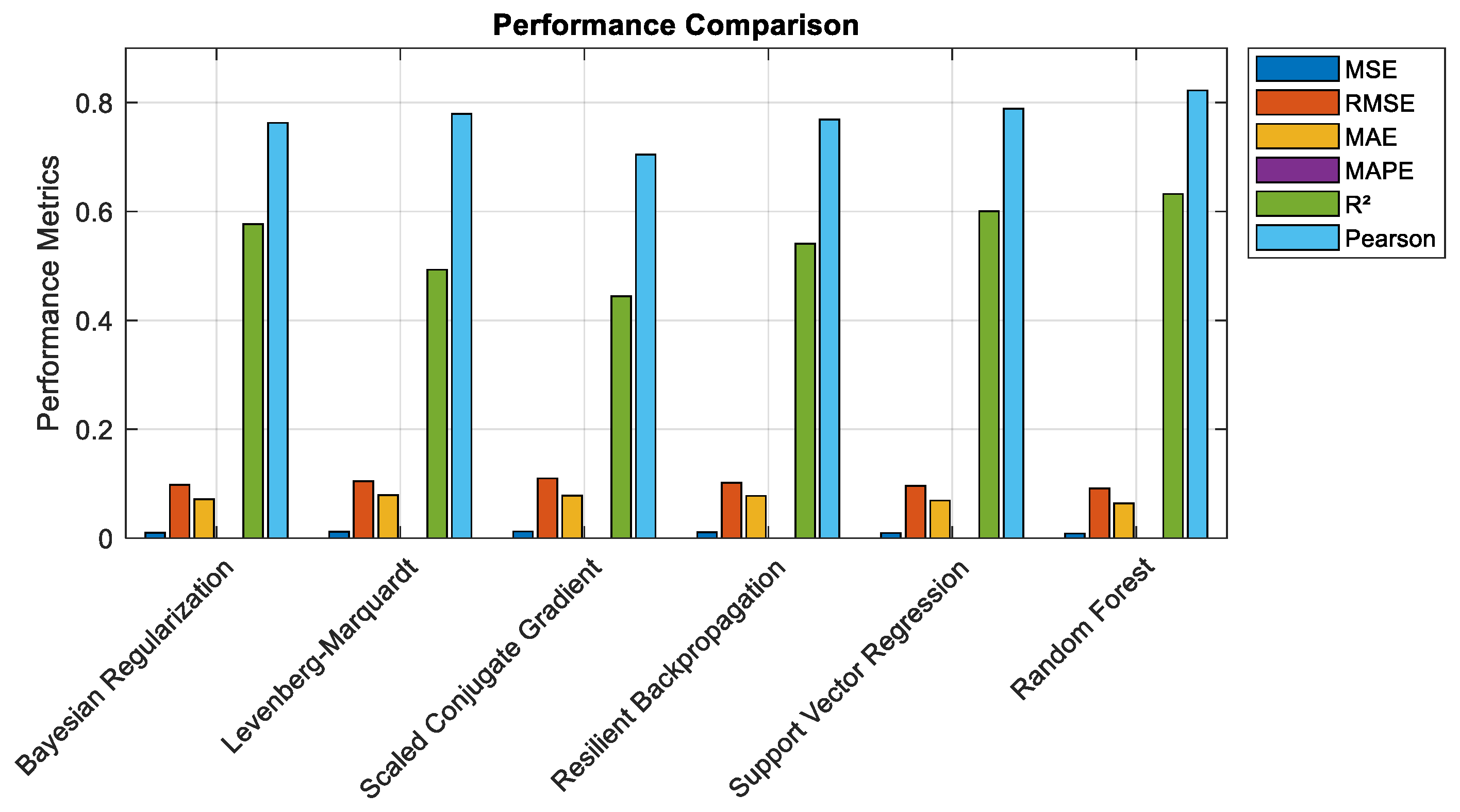
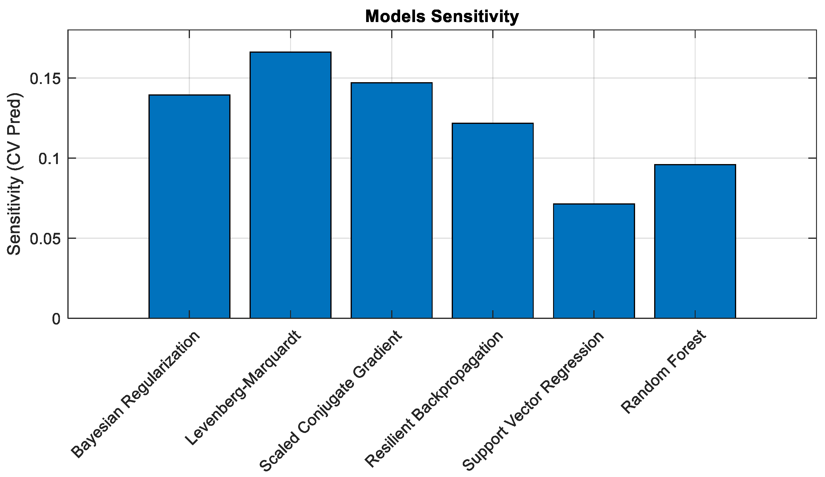
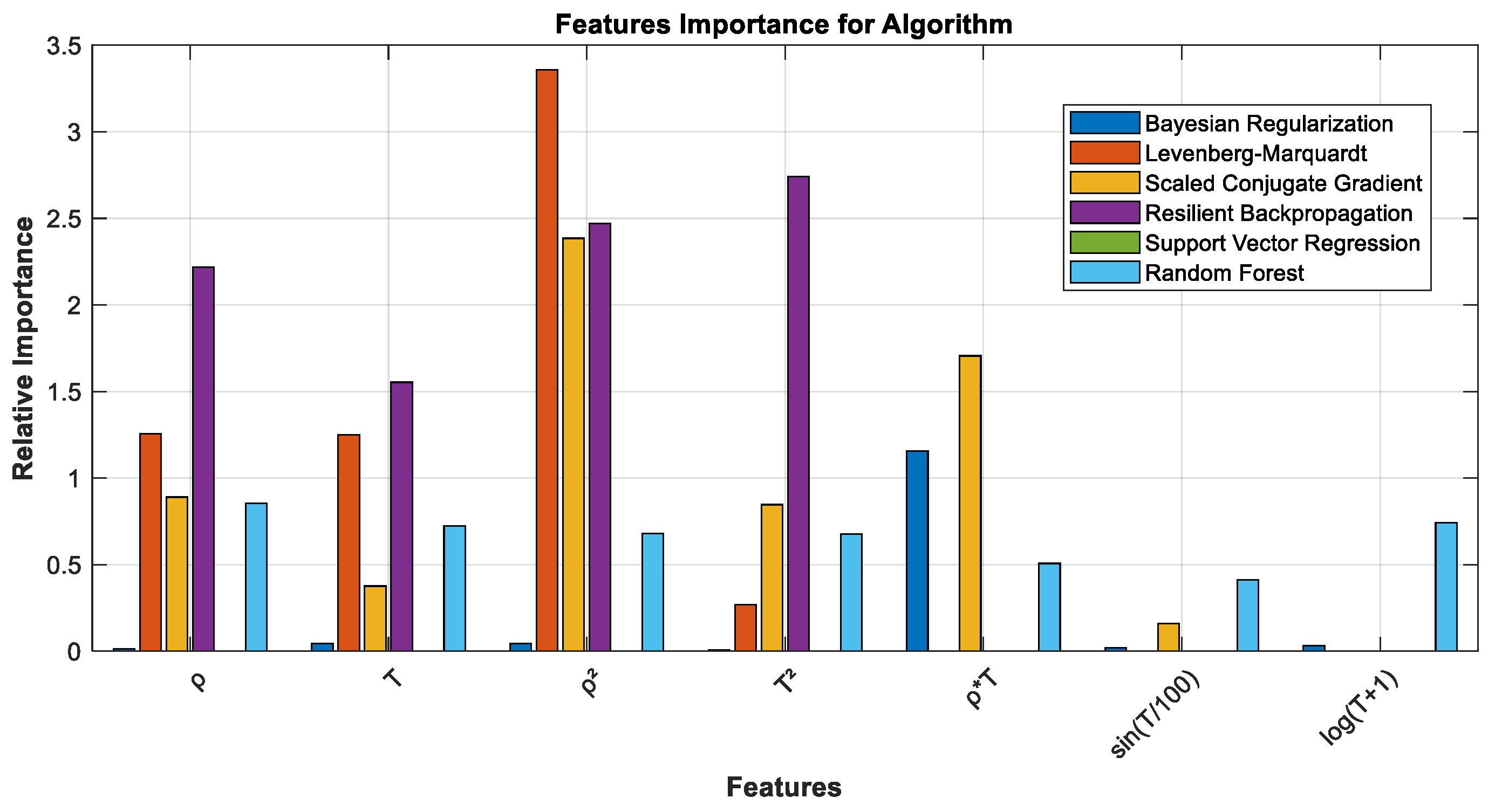
6.1. Performance Analysis

The comparison of results demonstrated several differences in performance terms among the algorithms that were implemented (Figure 8).

Resilient Backpropagation has proven to be the most effective method, achieving the lowest error metrics, with a mean squared error (MSE) of 38.87 MPa² and a mean absolute percentage error (MAPE) of 9.41%. This efficiency can be attributed to its adaptive learning rate mechanism, which effectively controls non-linear relationships. Bayesian Regularization exhibited similarly good results, with a mean squared error of 41.67 MPa², a root mean squared error of 6.46 MPa, and a mean absolute percentage error of 11.47%, achieved through effective complexity regularization.

Support Vector Regression utilizing a linear kernel demonstrated competitive performance, achieving a mean squared error (MSE) of 46.59 MPa² and a mean absolute percentage error (MAPE) of 9.65%. In contrast, the Random Forest model attained moderate performance levels, with an MSE of 49.70 MPa² and a MAPE of 11.95%, while providing consistent predictions across varying temperature ranges. The Levenberg–Marquardt and Scaled Conjugate Gradient methods exhibited significantly elevated error rates, with mean squared errors of 97.17 MPa² and 77.59 MPa², respectively. This indicates a lower accuracy in accurately representing complex thermo-mechanical behavior.

The sensitivity analysis results are shown in Figure 9 revealing interesting patterns of robustness.

Support Vector Regression exhibited the lowest sensitivity (CV ≈ 0.07), suggesting that it provides the most stable predictions in the face of variations in input data. The Random Forest model demonstrated a moderate level of sensitivity, with a coefficient of variation of approximately 0.09, whereas the Resilient Backpropagation model displayed a slightly greater degree of variation, indicated by a coefficient of variation of around 0.12. The Levenberg–Marquardt method exhibited the highest sensitivity, with a coefficient of variation of approximately 0.16. This finding indicates that the predictions are significantly influenced by variations in input, which may raise concerns regarding stability.

Feature importance analysis (Figure 10) identified temperature (T) and geometric ratio (ρ) as primary predictive variables across all models. Engineered features, particularly interaction term (ρ*T) and quadratic terms (T² and ρ²), contributed significantly to accuracy, especially for temperature extremes.

Uncertainty quantification revealed temperature-dependent patterns: low uncertainty (3.15–4.34%) in the 20–300 °C range, moderate uncertainty (5.79–7.18%) at 300–500 °C, and higher uncertainty (7.69–10.07%) above 500 °C. This progressive increase reflects growing material behavior complexity at elevated temperatures, consistently observed across all modeling approaches.

The validation process, which used independent experimental data, showed that model accuracy varied across different temperature ranges. The main results are summarized in

Table 4. Prediction and percent error compared to the experimental data.

Temperature	Compressive Strength [MPa]
	Experimental	BR	Error (%)	LM	Error (%)	SCG	Error (%)	RProp	Error (%)	SVR	Error (%)	RF	Error (%)
20	71.70	69.60	2.93	71.46	0.33	56.86	20.70	61.97	13.57	61.41	14.35	63.23	11.81
350	58.00	51.06	11.97	49.27	15.05	46.39	20.02	48.69	16.05	48.81	15.84	50.84	12.34
450	50.70	46.24	8.80	38.97	23.14	49.85	1.68	46.64	8.01	45.41	10.43	45.10	11.05
550	43.34	39.50	8.86	33.22	23.35	49.05	−13.17	41.48	4.29	42.02	3.05	40.23	7.18
650	35.78	32.22	9.95	27.74	22.47	41.70	−16.55	33.61	6.06	37.73	−5.45	31.94	10.73
750	28.22	25.07	11.16	27.35	3.08	36.92	−30.83	27.40	2.91	30.10	−6.66	25.46	9.78
800	24.44	21.00	14.08	27.35	−11.91	34.58	−41.49	22.41	8.31	24.35	0.37	23.78	2.70

.

At a temperature of 20 °C, the Levenberg–Marquardt method demonstrated good accuracy, achieving an error rate of 0.33%, while the Bayesian Regularization method followed with an error rate of 2.93%. Nonetheless, there was a notable change in performance patterns in response to rising temperatures.

The intermediate temperature range of 350–450 °C exhibited increased prediction errors, ranging from 11.97% to 20.02% at 350 °C, thereby highlighting the challenges experienced during thermal transitions. The Resilient Backpropagation method exhibited impressive performance at a temperature of 450 °C, achieving an error rate of 8.01%.

Support Vector Regression demonstrated remarkable accuracy at 800 °C, achieving an error rate of only 0.37%. In contrast, the Scaled Conjugate Gradient method exhibited an important deviation, with an error rate of −41.49%. The Random Forest model demonstrated stable performance, exhibiting errors consistently below 10% at a temperature of 750 °C.

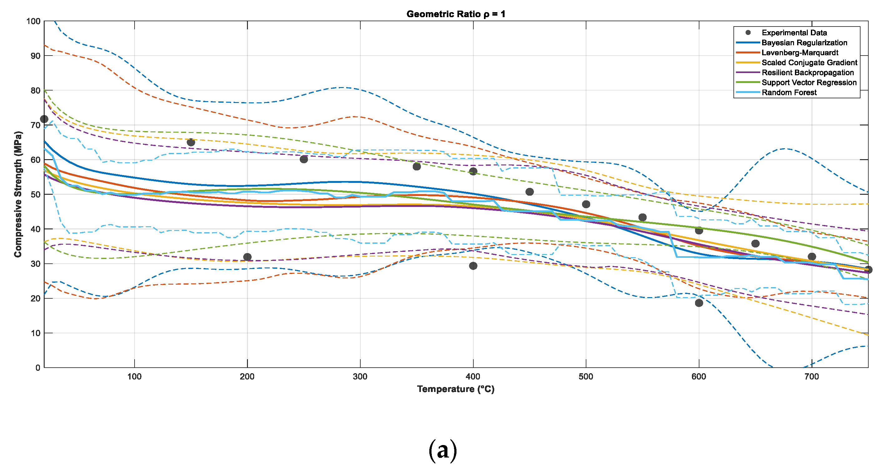
6.2. Prediction Results and Response Surfaces

The analysis of confidence intervals across various geometric configurations, as illustrated in Figure 11, indicated prevalent challenges associated with increased prediction uncertainty at temperatures exceeding 500 °C. The observed pattern, particularly evident in specimens exhibiting ρ = 1 and ρ = 3, indicates fundamental challenges in accurately representing material behavior in nearby thermal degradation thresholds.

The three-dimensional response surfaces illustrated in Figure 12 offer a complete visualization of thermo-mechanical behavior. This helps the identification of transition zones characterized by rapid changes in material behavior, the evaluation of geometric influences on thermal degradation patterns, and the identification of potential regions of instability. The continuous representation of parameter space fosters solid interpolation for geometric ratios among discretely evaluated values, which is beneficial for design choices as well as post-fire structural evaluations.

Resilient Backpropagation demonstrated superior overall metrics while offering smoother and more generalized predictions, making it well-suited for a variety of design applications. Bayesian Regularization demonstrated a noteworthy balance between accuracy and stability, proven by moderate error metrics (MSE = 41.67 MPa²) and consistent sensitivity (CV ≈ 0.14). This approach exhibited good surface continuity within the critical temperature range of 100–500 °C.

The strong performance of Support Vector Regression, despite its relatively simple architecture, indicates that the essential relationships governing SCC thermal degradation may be effectively represented through carefully designed linear separations within a transformed feature space. The increased uncertainty observed at elevated temperatures and extreme geometric ratios underscores significant areas that necessitate further investigation. This may require the development of more advanced modeling techniques or the acquisition of supplementary experimental data in these fields.

Finally, some limitations should be considered when applying these models. The dataset size, while sufficient for the comparative analysis performed, represents a constraint for broader generalization across diverse SCC formulations with varying mix designs and constituent materials. The modeling framework assumes relatively uniform specimen properties within each temperature group, which may not fully capture the inherent variability in concrete specimens due to factors such as aggregate distribution, curing conditions, or minor compositional variations. Generalization to other SCC types with significantly different formulations, aggregate characteristics, or additive combinations would require an expansion of the training dataset. Moreover, the prediction uncertainty increases notably at temperatures exceeding 500 °C, where complex physicochemical transformations occur, highlighting the need for additional experimental validation in extreme temperature ranges for critical structural assessment applications.

7. Conclusions

In this study, an effective and robust machine learning framework has been developed with the aim of predicting the residual compressive strength of SCC under elevated temperatures.

The comparative analysis of six machine learning approaches showed different performance characteristics across the temperature range. The Resilient Backpropagation algorithm proved to be the most effective method, getting the lowest overall prediction errors (MSE = 38.87 MPa², MAPE = 9.41%). This suggests its ability to capture the complex non-linear relationships associated with SCC thermal degradation. The Bayesian Regularization method offered a good alternative, achieving competitive accuracy (MSE = 41.67 MPa², MAPE = 11.47%) and good stability. Support Vector Regression shown a good efficiency reaching competitive performance (MSE = 46.59 MPa², MAPE = 9.65%) indicating that the key relationships in SCC thermal behavior can be effectively represented through carefully designed feature transformations. The Random Forest method provided consistent predictions offering valuable insight into feature importance and model interpretability.

The analysis of the training database identified key data characteristics that guided the selection of algorithms. The identification of heteroscedastic data distribution (Levene test, p < 0.001), non-normal variable distributions, and strong non-linear correlations (Spearman ρ = −0.68 vs. Pearson r = −0.61) underscores the need for advanced machine learning approaches rather than traditional parametric methods.

The experimental validation campaign using SCC specimens tested at temperatures up to 800 °C provided independent verification of model performance. The results demonstrated varying accuracy across temperature ranges: excellent prediction capability at moderate temperatures (20–400 °C) with errors typically below 15% and increasing uncertainty at elevated temperatures (>500 °C) where prediction errors ranged up to 23.35%. This pattern reflects the inherent complexity of material behavior approaching thermal degradation thresholds and provides important guidance for practical applications. The uncertainty quantification analysis revealed systematic patterns in prediction reliability, with confidence intervals ranging from 3.15–4.34% at low temperatures to 7.69–10.07% at extreme conditions. This graduated uncertainty assessment enables practitioners to make informed decisions about model application limits and required safety factors.

The proposed framework provides notable practical benefits for structural fire engineering by significantly minimizing testing needs for material characterization, resulting in substantial time and cost efficiencies. The models serve as effective instruments for swift post-fire evaluations of damaged structures, allowing engineers to assess residual capacity without the need for extensive destructive testing. This capability is especially important for historic buildings or structures subjected to extreme conditions. The three-dimensional response surfaces produced by the models facilitate an in-depth examination of the parameter space for optimized design choices. Additionally, the analysis of confidence intervals offers quantitative uncertainty bounds that can be integrated into probabilistic safety evaluations and risk management strategies.

This study has shown the effectiveness of machine learning methods in predicting the thermal behavior of SCC; however, several limitations should be acknowledged. The heightened prediction uncertainty at temperatures exceeding 500 °C underscores the necessity for further experimental data in extreme temperature ranges. The existing framework emphasizes compressive strength as the main response variable. Future investigations should broaden this approach to include additional mechanical properties, including tensile strength, elastic modulus, and fracture parameters.

The geometric ratio parameter effectively captures specimen size effects; however, it could be improved by incorporating additional geometric variables, such as surface area-to-volume ratios or more complex shape factors. The incorporation of mixture composition parameters, such as cement content, aggregate type, and additives, may substantially improve the model applicability across various SCC formulations.

References

1. United Nation Office for Disaster Risk Reduction (UNDRR) Fires in Europe Fuelled by Urbanisation and Climate Change. Available online: https://www.undrr.org/news/fires-europe-fuelled-urbanisation-and-climate-change (accessed on 10 April 2025).
2. European Innovation Council. The European Prize for Humanitarian Innovation. Available online: https://eic.ec.europa.eu/eic-prizes/european-prize-humanitarian-innovation_en (accessed on 15 June 2024).
3. Ruíz, M.A.; Mack-Vergara, Y.L. Resilient and Sustainable Housing Models against Climate Change: A Review. Sustainability 2023, 15, 13544. [Google Scholar] [CrossRef]
4. Peng, T.; Lemay, L.; Cody, B. Concrete Building Systems: Disaster Resilient Solutions for Safer Communities. In Proceedings of the 1st Residential Building Design & Construction Conference, Bethlehem, PA, USA, 20–21 February 2013; pp. 46–55. [Google Scholar]
5. Uysal, M.; Tanyildizi, H. Estimation of Compressive Strength of Self Compacting Concrete Containing Polypropylene Fiber and Mineral Additives Exposed to High Temperature Using Artificial Neural Network. Constr. Build. Mater. 2012, 27, 404–414. [Google Scholar] [CrossRef]
6. Ealiyas Mathews, M.; Kiran, T.; Anand, N.; Lubloy, E.; Naser, M.Z.; Prince Arulraj, G. Effect of Protective Coating on Axial Resistance and Residual Capacity of Self-Compacting Concrete Columns Exposed to Standard Fire. Eng. Struct. 2022, 264, 114444. [Google Scholar] [CrossRef]
7. La Scala, A.; Loprieno, P.; Ivorra, S.; Foti, D.; La Scala, M. Modal Analysis of a Fire-Damaged Masonry Vault. Fire 2024, 7, 194. [Google Scholar] [CrossRef]
8. Mathews, M.E.; Andrushia, A.D.; Kiran, T.; Yadav, B.S.K.; Kanagaraj, B.; Anand, N. Structural Response of Self-Compacting Concrete Beams under Elevated Temperature. In Proceedings of the Materials Today: Proceedings; Elsevier Ltd.: Amsterdam, The Netherlands, 2021; Volume 49, pp. 1246–1254. [Google Scholar]
9. Khaliq, W.; Kodur, V. Thermal and Mechanical Properties of Fiber Reinforced High Performance Self-Consolidating Concrete at Elevated Temperatures. Cem. Concr. Res. 2011, 41, 1112–1122. [Google Scholar] [CrossRef]
10. Mansoor, J.; Shah, S.A.R.; Khan, M.M.; Sadiq, A.N.; Anwar, M.K.; Siddiq, M.U.; Ahmad, H. Analysis of Mechanical Properties of Self Compacted Concrete by Partial Replacement of Cement with Industrial Wastes under Elevated Temperature. Appl. Sci. 2018, 8, 364. [Google Scholar] [CrossRef]
11. Scala, M.L.; Trovato, M.; Torelli, F.; La Scala, M.; Trovato, M.; Torelli, F. A Neural Network-Based Method for Voltage Security Monitoring. IEEE Trans. Power Syst. 1996, 11, 1332–1341. [Google Scholar] [CrossRef]
12. Carnimeo, L.; Foti, D.; Potenza, F. On Protecting and Managing Slender Buildings from Risk Events via a Multitask Monitoring Network. In Proceedings of the SHMII 2015—7th International Conference on Structural Health Monitoring of Intelligent Infrastructure, Torino, Italy, 1–3 July 2015. [Google Scholar]
13. Carnimeo, L.; Foti, D.; Ivorra, S. On Modeling an Innovative Monitoring Network for Protecting and Managing Cultural Heritage from Risk Events. Key Eng. Mater. 2015, 628, 243–249. [Google Scholar] [CrossRef]
14. Rizzo, F.; Caracoglia, L.; Piccardo, G. Examining Wind-Induced Floor Accelerations in an Unconventionally Shaped, High-Rise Building for the Design of “Smart” Screen Walls. J. Build. Eng. 2021, 43, 103115. [Google Scholar] [CrossRef]
15. Rizzo, F.; Barbato, M.; Sepe, V. Shape Dependence of Wind Pressure Peak Factor Statistics in Hyperbolic Paraboloid Roofs. J. Build. Eng. 2021, 44, 103203. [Google Scholar] [CrossRef]
16. Rizzo, F. Investigation of the Time Dependence of Wind-Induced Aeroelastic Response on a Scale Model of a High-Rise Building. Appl. Sci. 2021, 11, 3315. [Google Scholar] [CrossRef]
17. Rizzo, F.; Sadhu, A.; Abasi, A.; Pistol, A.; Flaga, Ł.; Venanzi, I.; Ubertini, F. Construction and Dynamic Identification of Aeroelastic Test Models for Flexible Roofs. Arch. Civ. Mech. Eng. 2022, 23, 16. [Google Scholar] [CrossRef]
18. Scala, A.L.; Rizzo, F.; Carnimeo, L.; Chorro, S.I.; Foti, D. A Proposal of a Neural Predictor of Residual Compressive Strength in an SCC Exposed to High Temperatures for Resilient Housing. In Proceedings of the 2024 IEEE International Humanitarian Technologies Conference (IHTC), Bari, Italy, 27–30 November 2024; pp. 1–6. [Google Scholar]
19. Ivorra, S.; Brotóns, V.; Foti, D.; Diaferio, M. A Preliminary Approach of Dynamic Identification of Slender Buildings by Neuronal Networks. Int. J. Non Linear Mech. 2016, 80, 183–189. [Google Scholar] [CrossRef]
20. Decreto Ministeriale 14 Ottobre 2021—Approvazione di Norme Tecniche di Prevenzione incendi per gli Edifici Sottoposti a Tutela ai Sensi del Decreto Legislativo 22 Gennaio 2004, n. 42, Aperti al Pubblico, Contenenti una o più Attività ri-Comprese nell’all. Italy: Ministero dell’Interno. 2021. Available online: https://www.tuttoprevenzioneincendi.it/images/Norme/DM_14_10_2021.pdf (accessed on 24 April 2025).
21. RILEM Technical Committee 200-HTC. Recommendation of RILEM TC 200-HTC: Mechanical concrete properties at high tem-peratures—Modelling and applications. Mater. Struct. 2007, 40, 841–853. [Google Scholar] [CrossRef]
22. Lazarevska, M.; Knezevic, M.; Cvetkovska, M.; Trombeva-Gavriloska, A. Application of Artificial Neural Networks in Civil Engineering. Teh. Vjesn. 2014, 21, 1353–1359. [Google Scholar]
23. Chojaczyk, A.A.; Teixeira, A.P.; Neves, L.C.; Cardoso, J.B.; Guedes Soares, C. Review and Application of Artificial Neural Networks Models in Reliability Analysis of Steel Structures. Struct. Saf. 2015, 52, 78–89. [Google Scholar] [CrossRef]
24. Yuen, K.-V. Bayesian Methods for Structural Dynamics and Civil Engineering; John Wiley & Sons: Singapore, 2010; ISBN 978-0-470-82454-2. [Google Scholar]
25. Lopez Peña, F.; Díaz Casás, V.; Gosset, A.; Duro, R.J. A Surrogate Method Based on the Enhancement of Low Fidelity Computational Fluid Dynamics Approximations by Artificial Neural Networks. Comput. Fluids 2012, 58, 112–119. [Google Scholar] [CrossRef]
26. Kocabaş, F.; Ünal, S.; Ünal, B. A Neural Network Approach for Prediction of Critical Submergence of an Intake in Still Water and Open Channel Flow for Permeable and Impermeable Bottom. Comput. Fluids 2008, 37, 1040–1046. [Google Scholar] [CrossRef]
27. Mata, J. Interpretation of Concrete Dam Behaviour with Artificial Neural Network and Multiple Linear Regression Models. Eng. Struct. 2011, 33, 903–910. [Google Scholar] [CrossRef]
28. Nourani, V.; Komasi, M.; Mano, A. A Multivariate ANN-Wavelet Approach for Rainfall-Runoff Modeling. Water Resour. Manag. 2009, 23, 2877–2894. [Google Scholar] [CrossRef]
29. Shahin, M.A.; Jaksa, M.B.; Maier, H.R. Artificial Neural Network Applications in Geotechnical Engineering. Aust. Geomech. J. 2001, 36, 49–62. [Google Scholar]
30. Gomes, H.M.; Awruch, A.M.; Lopes, P.A.M. Reliability Based Optimization of Laminated Composite Structures Using Genetic Algorithms and Artificial Neural Networks. Struct. Saf. 2011, 33, 186–195. [Google Scholar] [CrossRef]
31. Le, V.; Caracoglia, L. A Neural Network Surrogate Model for the Performance Assessment of a Vertical Structure Subjected to Non-Stationary, Tornadic Wind Loads. Comput. Struct. 2020, 231, 106208. [Google Scholar] [CrossRef]
32. Seo, D.W.; Caracoglia, L. Estimation of Torsional-Flutter Probability in Flexible Bridges Considering Randomness in Flutter Derivatives. Eng. Struct. 2011, 33, 2284–2296. [Google Scholar] [CrossRef]
33. Rizzo, F.; Caracoglia, L. Artificial Neural Network Model to Predict the Flutter Velocity of Suspension Bridges. Comput. Struct. 2020, 233, 106236. [Google Scholar] [CrossRef]
34. Rizzo, F.; Caracoglia, L. Examination of Artificial Neural Networks to Predict Wind-Induced Displacements of Cable Net Roofs. Eng. Struct. 2021, 245, 112956. [Google Scholar] [CrossRef]
35. Bakhary, N.; Hao, H.; Deeks, A.J. Damage Detection Using Artificial Neural Network with Consideration of Uncertainties. Eng. Struct. 2007, 29, 2806–2815. [Google Scholar] [CrossRef]
36. Deng, J.; Gu, D.; Li, X.; Yue, Z.Q. Structural Reliability Analysis for Implicit Performance Functions Using Artificial Neural Network. Struct. Saf. 2005, 27, 25–48. [Google Scholar] [CrossRef]
37. Pathirage, C.S.N.; Li, J.; Li, L.; Hao, H.; Liu, W.; Ni, P. Structural Damage Identification Based on Autoencoder Neural Networks and Deep Learning. Eng. Struct. 2018, 172, 13–28. [Google Scholar] [CrossRef]
38. Möller, O.; Foschi, R.O.; Quiroz, L.M.; Rubinstein, M. Structural Optimization for Performance-Based Design in Earthquake Engineering: Applications of Neural Networks. Struct. Saf. 2009, 31, 490–499. [Google Scholar] [CrossRef]
39. Asteris, P.G.; Nikoo, M. Artificial Bee Colony-Based Neural Network for the Prediction of the Fundamental Period of Infilled Frame Structures. Neural Comput. Appl. 2019, 31, 4837–4847. [Google Scholar] [CrossRef]
40. Papadrakakis, M.; Lagaros, N.D. Reliability-Based Structural Optimization Using Neural Networks and Monte Carlo Simulation. Comput. Methods Appl. Mech. Eng. 2002, 191, 3491–3507. [Google Scholar] [CrossRef]
41. Chen, S.Z.; Zhang, S.Y.; Han, W.S.; Wu, G. Ensemble Learning Based Approach for FRP-Concrete Bond Strength Prediction. Constr. Build. Mater. 2021, 302, 124230. [Google Scholar] [CrossRef]
42. Güçlüer, K.; Özbeyaz, A.; Göymen, S.; Günaydın, O. A Comparative Investigation Using Machine Learning Methods for Concrete Compressive Strength Estimation. Mater. Today Commun. 2021, 27, 102278. [Google Scholar] [CrossRef]
43. Chou, J.S.; Pham, A.D. Enhanced Artificial Intelligence for Ensemble Approach to Predicting High Performance Concrete Compressive Strength. Constr. Build. Mater. 2013, 49, 554–563. [Google Scholar] [CrossRef]
44. Chen, B.T.; Chang, T.P.; Shih, J.Y.; Wang, J.J. Estimation of Exposed Temperature for Fire-Damaged Concrete Using Support Vector Machine. Comput. Mater. Sci. 2009, 44, 913–920. [Google Scholar] [CrossRef]
45. Mangalathu, S.; Hwang, S.H.; Jeon, J.S. Failure Mode and Effects Analysis of RC Members Based on Machine-Learning-Based SHapley Additive ExPlanations (SHAP) Approach. Eng. Struct. 2020, 219, 110927. [Google Scholar] [CrossRef]
46. Amini, K.; Jalalpour, M.; Delatte, N. Advancing Concrete Strength Prediction Using Non-Destructive Testing: Development and Verification of a Generalizable Model. Constr. Build. Mater. 2016, 102, 762–768. [Google Scholar] [CrossRef]
47. Nguyen, T.H.; Tran, D.H.; Nguyen, N.M.; Vuong, H.T.; Chien-Cheng, C.; Cao, M.T. Accurately Predicting the Mechanical Behavior of Deteriorated Reinforced Concrete Components Using Natural Intelligence-Integrated Machine Learners. Constr. Build. Mater. 2023, 408, 133753. [Google Scholar] [CrossRef]
48. Ushizima, D.; Xu, K.; Monteiro, P.J.M. Materials Data Science for Microstructural Characterization of Archaeological Concrete. MRS Adv. 2020, 5, 305–318. [Google Scholar] [CrossRef]
49. Mishra, M. Machine Learning Techniques for Structural Health Monitoring of Heritage Buildings: A State-of-the-Art Review and Case Studies. J. Cult. Herit. 2021, 47, 227–245. [Google Scholar] [CrossRef]
50. Dietterich, T.G.; Kolen, J.F.; Pollack, J.B. Ensemble Methods in Machine Learning BT—Multiple Classifier Systems. In Proceedings of the Complex Systems; Springer: Berlin/Heidelberg, Germany, 2000; Volume 4, pp. 1–15. [Google Scholar]
51. Zhou, Z.-H. Ensemble Methods: Foundations and Algorithms, 1st ed.; Chapman and Hall/CRC: Boca Raton, FL, USA, 2012. [Google Scholar]
52. Hansen, L.K.; Salamon, P. Neural Network Ensembles. IEEE Trans. Pattern Anal. Mach. Intell. 1990, 12, 993–1001. [Google Scholar] [CrossRef]
53. Polikar, R. Ensemble Learning. In Ensemble Machine Learning: Methods and Applications; Zhang, C., Ma, Y., Eds.; Springer: New York, NY, USA, 2012; pp. 1–34. ISBN 978-1-4419-9326-7. [Google Scholar]
54. Alharthy, S.E.; Mostafa, M.A. Mechanical and Thermal Charactristics of Self-Compacting Concrete Produced with Blast Furnace Slag and Fly Ash. HBRC J. 2020, 16, 283–298. [Google Scholar] [CrossRef]
55. Bamonte, P.; Gambarova, P.G. A Study on the Mechanical Properties of Self-Compacting Concrete at High Temperature and after Cooling. Mater. Struct. 2012, 45, 1375–1387. [Google Scholar] [CrossRef]
56. Persson, B. A Comparison between Mechanical Properties of Self-Compacting Concrete and the Corresponding Properties of Normal Concrete. Cem. Concr. Res. 2001, 31, 193–198. [Google Scholar] [CrossRef]
57. Farhad, A.; Junbo, S.; Guanqi, H. Mechanical Behavior of Fiber-Reinforced Self-Compacting Rubberized Concrete Exposed to Elevated Temperatures. J. Mater. Civ. Eng. 2019, 31, 4019302. [Google Scholar] [CrossRef]
58. Mňahončáková, E.; Pavlíková, M.; Grzeszczyk, S.; Rovnanı´ková, P.; Černý, R. Hydric, Thermal and Mechanical Properties of Self-Compacting Concrete Containing Different Fillers. Constr. Build. Mater. 2008, 22, 1594–1600. [Google Scholar] [CrossRef]
59. Jiao, P.; Roy, M.; Barri, K.; Zhu, R.; Ray, I.; Alavi, A.H.; Hu, X.; Li, B.; Mo, Y.; Alselwi, O.; et al. Machine Learning Prediction Models to Evaluate the Strength of Recycled Aggregate Concrete. Materials 2022, 15, 3605. [Google Scholar] [CrossRef]
60. Shahrokhishahraki, M.; Malekpour, M.; Mirvalad, S.; Faraone, G.; Liu, K.-H.; Xie, T.-Y.; Cai, Z.-K.; Chen, G.-M.; Zhao, X.-Y.; Nguyen, T.-H.; et al. A Comparative Study of Random Forest and Genetic Engineering Programming for the Prediction of Compressive Strength of High Strength Concrete (HSC). J. Build. Eng. 2024, 10, 108160. [Google Scholar] [CrossRef]
61. Mai, H.V.T.; Nguyen, M.H.; Ly, H.B. Development of Machine Learning Methods to Predict the Compressive Strength of Fiber-Reinforced Self-Compacting Concrete and Sensitivity Analysis. Constr. Build. Mater. 2023, 367, 130339. [Google Scholar] [CrossRef]
62. Liu, Y.; Cao, Y.; Wang, L.; Chen, Z.S.; Qin, Y. Prediction of the Durability of High-Performance Concrete Using an Integrated RF-LSSVM Model. Constr. Build. Mater. 2022, 356, 129232. [Google Scholar] [CrossRef]
63. Rajakarunakaran, S.A.; Lourdu, A.R.; Muthusamy, S.; Panchal, H.; Jawad Alrubaie, A.; Musa Jaber, M.; Ali, M.H.; Tlili, I.; Maseleno, A.; Majdi, A.; et al. Prediction of Strength and Analysis in Self-Compacting Concrete Using Machine Learning Based Regression Techniques. Adv. Eng. Softw. 2022, 173, 103267. [Google Scholar] [CrossRef]
64. de-Prado-Gil, J.; Palencia, C.; Silva-Monteiro, N.; Martínez-García, R. To Predict the Compressive Strength of Self Compacting Concrete with Recycled Aggregates Utilizing Ensemble Machine Learning Models. Case Stud. Constr. Mater. 2022, 16, e01046. [Google Scholar] [CrossRef]
65. Malami, S.I.; Anwar, F.H.; Abdulrahman, S.; Haruna, S.I.; Ali, S.I.A.; Abba, S.I. Implementation of Hybrid Neuro-Fuzzy and Self-Turning Predictive Model for the Prediction of Concrete Carbonation Depth: A Soft Computing Technique. Results Eng. 2021, 10, 100228. [Google Scholar] [CrossRef]
66. Arbaoui, A. Wavelet-Based Multiresolution Analysis Coupled with Deep Learning to Efficiently Monitor Cracks in Concrete. Frat. Ed. Integrità Strutt. 2021, 15, 33–47. [Google Scholar] [CrossRef]
67. Chu, H.H.; Khan, M.A.; Javed, M.; Zafar, A.; Ijaz Khan, M.; Alabduljabbar, H.; Qayyum, S. Sustainable Use of Fly-Ash: Use of Gene-Expression Programming (GEP) and Multi-Expression Programming (MEP) for Forecasting the Compressive Strength Geopolymer Concrete. Ain Shams Eng. J. 2021, 12, 3603–3617. [Google Scholar] [CrossRef]
68. Ziolkowski, P.; Niedostatkiewicz, M.; Padmapoorani, P.; Senthilkumar, S.; Mohanraj, R. Machine Learning Techniques in Concrete Mix Design. Materials 2019, 12, 1256. [Google Scholar] [CrossRef]
69. Li, Z.; Yoon, J.; Zhang, R.; Rajabipour, F.; Srubar, W.V.; Dabo, I.; Radlińska, A. Machine Learning in Concrete Science: Applications, Challenges, and Best Practices. NPJ Comput. Mater. 2022, 8, 127. [Google Scholar] [CrossRef]
70. Kaveh, A.; Khavaninzadeh, N. Efficient Training of Two ANNs Using Four Meta-Heuristic Algorithms for Predicting the FRP Strength. Structures 2023, 52, 256–272. [Google Scholar] [CrossRef]
71. Song, H.; Ahmad, A.; Farooq, F.; Ostrowski, K.A.; Maślak, M.; Czarnecki, S.; Aslam, F. Predicting the Compressive Strength of Concrete with Fly Ash Admixture Using Machine Learning Algorithms. Constr. Build. Mater. 2021, 308, 125021. [Google Scholar] [CrossRef]
72. Farooq, F.; Ahmed, W.; Akbar, A.; Aslam, F.; Alyousef, R. Predictive Modeling for Sustainable High-Performance Concrete from Industrial Wastes: A Comparison and Optimization of Models Using Ensemble Learners. J. Clean. Prod. 2021, 292, 126032. [Google Scholar] [CrossRef]
73. Maherian, M.F.; Baran, S.; Bicakci, S.N.; Toreyin, B.U.; Atahan, H.N. Machine Learning-Based Compressive Strength Estimation in Nano Silica-Modified Concrete. Constr. Build. Mater. 2023, 408, 133684. [Google Scholar] [CrossRef]
74. Feng, D.C.; Liu, Z.T.; Wang, X.D.; Chen, Y.; Chang, J.Q.; Wei, D.F.; Jiang, Z.M. Machine Learning-Based Compressive Strength Prediction for Concrete: An Adaptive Boosting Approach. Constr. Build. Mater. 2020, 230, 117000. [Google Scholar] [CrossRef]
75. Mohtasham Moein, M.; Saradar, A.; Rahmati, K.; Ghasemzadeh Mousavinejad, S.H.; Bristow, J.; Aramali, V.; Karakouzian, M. Predictive Models for Concrete Properties Using Machine Learning and Deep Learning Approaches: A Review. J. Build. Eng. 2023, 63, 105444. [Google Scholar] [CrossRef]
76. Yeh, I.C. Modeling of Strength of High-Performance Concrete Using Artificial Neural Networks. Cem. Concr. Res. 1998, 28, 1797–1808. [Google Scholar] [CrossRef]
77. Khademi, F.; Akbari, M.; Jamal, S.M.; Nikoo, M. Multiple Linear Regression, Artificial Neural Network, and Fuzzy Logic Prediction of 28 Days Compressive Strength of Concrete. Front. Struct. Civ. Eng. 2017, 11, 90–99. [Google Scholar] [CrossRef]
78. Ashrafian, A.; Taheri Amiri, M.J.; Rezaie-Balf, M.; Ozbakkaloglu, T.; Lotfi-Omran, O. Prediction of Compressive Strength and Ultrasonic Pulse Velocity of Fiber Reinforced Concrete Incorporating Nano Silica Using Heuristic Regression Methods. Constr. Build. Mater. 2018, 190, 479–494. [Google Scholar] [CrossRef]
79. Mai, H.-V.T.; Nguyen, T.-A.; Ly, H.-B.; Tran, V.Q. Prediction Compressive Strength of Concrete Containing GGBFS Using Random Forest Model. Adv. Civ. Eng. 2021, 2021, 6671448. [Google Scholar] [CrossRef]
80. Li, Y.; Hishamuddin, F.N.S.; Mohammed, A.S.; Armaghani, D.J.; Ulrikh, D.V.; Dehghanbanadaki, A.; Azizi, A. The Effects of Rock Index Tests on Prediction of Tensile Strength of Granitic Samples: A Neuro-Fuzzy Intelligent System. Sustainability 2021, 13, 10541. [Google Scholar] [CrossRef]
81. Asteris, P.G.; Lourenço, P.B.; Roussis, P.C.; Elpida Adami, C.; Armaghani, D.J.; Cavaleri, L.; Chalioris, C.E.; Hajihassani, M.; Lemonis, M.E.; Mohammed, A.S.; et al. Revealing the Nature of Metakaolin-Based Concrete Materials Using Artificial Intelligence Techniques. Constr. Build. Mater. 2022, 322, 126500. [Google Scholar] [CrossRef]
82. Ali, R.; Muayad, M.; Mohammed, A.S.; Asteris, P.G. Analysis and Prediction of the Effect of Nanosilica on the Compressive Strength of Concrete with Different Mix Proportions and Specimen Sizes Using Various Numerical Approaches. Struct. Concr. 2023, 24, 4161–4184. [Google Scholar] [CrossRef]
83. Chen, C.-H.; Wu, J.-C.; Chen, J.-H. Prediction of Flutter Derivatives by Artificial Neural Networks. J. Wind. Eng. Ind. Aerodyn.—J. Wind Eng. Ind. Aerodyn. 2008, 96, 1925–1937. [Google Scholar] [CrossRef]
84. MacKay, D.J.C.; Foresee, F.D.; Hagan, M.T. Bayesian Interpolation. Neural Comput. 1992, 4, 415–447. [Google Scholar] [CrossRef]
85. Dan Foresee, F.; Hagan, M.T. Gauss-Newton Approximation to Bayesian Learning. In Proceedings of the International Conference on Neural Networks (ICNN’97), Houston, TX, USA, 9–12 June 1997; Volume 3, pp. 1930–1935. [Google Scholar]
86. MATLAB Manual. Version: 9.13.0 (R2022b), The MathWorks Inc.: Natick, MA, USA, 2022.
87. Riedmiller, M.; Braun, H. RPROP—A Fast Adaptive Learning Algorithm. 1992. Available online: https://api.semanticscholar.org/CorpusID:53929455 (accessed on 1 January 2025).
88. Benjeddou, O.; Katman, H.Y.; Jedidi, M.; Mashaan, N. Experimental Investigation of the High Temperatures Effects on Self-Compacting Concrete Properties. Buildings 2022, 12, 729. [Google Scholar] [CrossRef]
89. Rukavina, M.J.; Gabrijel, I.; Grubeša, I.N.; Mladenovič, A. Residual Compressive Behavior of Self-Compacting Concrete after High Temperature Exposure-Influence of Binder Materials. Materials 2022, 15, 2222. [Google Scholar] [CrossRef]
90. Bamonte, P.; Gambarova, P.G. High-Temperature Behavior of SCC in Compression: Comparative Study on Recent Experimental Campaigns. J. Mater. Civ. Eng. 2016, 28. [Google Scholar] [CrossRef]
91. Khaliq, W.; Kodur, V. Effectiveness of Polypropylene and Steel Fibers in Enhancing Fire Resistance of High-Strength Concrete Columns. J. Struct. Eng. 2018, 144, 4017224. [Google Scholar] [CrossRef]
92. Bogas, J.A.; Gomes, A.; Pereira, M.F.C. Self-Compacting Lightweight Concrete Produced with Expanded Clay Aggregate. Constr. Build. Mater. 2012, 35, 1013–1022. [Google Scholar] [CrossRef]
93. Al-Martini, S.; Nehdi, M. Effects of Heat and Mixing Time on Self-Compacting Concrete. Proc. Inst. Civ. Eng. Constr. Mater. 2010, 163, 175–182. [Google Scholar] [CrossRef]
94. Raif Boğa, A.; Karakurt, C.; Ferdi Şenol, A. The Effect of Elevated Temperature on the Properties of SCC’s Produced with Different Types of Fibers. Constr. Build. Mater. 2022, 340, 127803. [Google Scholar] [CrossRef]
95. Surya, T.R.; Prakash, M.; Satyanarayanan, K.S.; Celestine, A.K.; Parthasarathi, N. Compressive Strength of Self Compacting Concrete under Elevated Temperature. In Proceedings of the Materials Today: Proceedings; Elsevier Ltd.: Amsterdam, The Netherlands, 2020; Volume 40, pp. S83–S87. [Google Scholar]
96. Tao, J.; Yuan, Y.; Taerwe, L. Compressive Strength of Self-Compacting Concrete during High-Temperature Exposure. J. Mater. Civ. Eng. 2010, 22, 1005–1011. [Google Scholar] [CrossRef]
97. Sideris, K.K. Mechanical Characteristics of Self-Consolidating Concretes Exposed to Elevated Temperatures. J. Mater. Civ. Eng. 2007, 19, 648–654. [Google Scholar] [CrossRef]
98. Ente Nazionale Italiano di Unificazione. Prova sul Calcestruzzo Autocompattante Fresco—Determinazione del Tempo di Efflusso Dall’imbuto (UNI 11042:2003). 2003. Available online: https://store.uni.com/uni-11042-2003 (accessed on 24 April 2025).
99. Ente Nazionale Italiano di Unificazione. Calcestruzzo—Specificazione, Prestazione, Produzione e Conformità (UNI EN 206:2021). 2022. Available online: https://store.uni.com/uni-en-206-2021 (accessed on 24 April 2025).
Figure 1. Literature data used for training.
Fire 08 00289 g001
Figure 2. Parameters boxplot (a) and parameter statistic distribution (b). In the boxplots, red plus signs (+) represent outliers.
Fire 08 00289 g002
Figure 3. Levene test for variances. Blue boxes represent the data distribution through quartiles, red horizontal lines indicate the median of each distribution, and red plus signs (+) represent outliers.
Fire 08 00289 g003
Figure 4. Neural network basic architecture.
Fire 08 00289 g004
Figure 5. Cracked specimens after thermal exposure to 650 °C and cooling.
Fire 08 00289 g005
Figure 6. Compressive test on a sample heated to 800 °C.
Fire 08 00289 g006
Figure 7. Resistance determined experimentally for SCC for specimens with ρ = 1 and 2.
Fire 08 00289 g007
Figure 8. Metrics comparison for each algorithm.
Fire 08 00289 g008
Figure 9. Sensitivity analysis results.
Fire 08 00289 g009
Figure 10. Feature importance analysis.
Fire 08 00289 g010
Figure 11. Prediction results (continuous lines) and confidence intervals (dotted lines) for ρ = 1 (a), ρ = 2 (b), ρ = 3 (c).
Fire 08 00289 g011aFire 08 00289 g011b
Figure 12. Predicted surfaces for trainbr (a), trainlm (b), trainscg (c), trainrp (d), fitrsvm (e), and TreeBagger (f).
Fire 08 00289 g012