Potential Flow of Unburned Mixture and Combustion Products After Ignition in a Two-Dimensional Approximation

Abstract

The evolution of a flame front in a channel was considered in a two-dimensional approximation. In the approximation of the potential flow of combustion products and unburned mixture, the formation of a finger-shaped flame was considered after ignition at the closed end of the channel, on the channel axis, and on the side wall of the channel. The prerequisites for the formation of a tulip-shaped flame were considered in a potential approximation. The method of conformal mapping was used. Simple analytical functions were used that allowed equipotential lines and streamlines to be transformed. The shape of the flame front was obtained. The analytical results were compared with the experimentally obtained results of the flame front evolution and with numerical results obtained by other authors. The conditions for the applicability of the conformal mapping to a reacting gas mixture were given.

1. Introduction

Determining the patterns of flame front propagation in pre-mixed gas mixtures is one of the most important tasks, both in practical applications and for ensuring the explosion safety of flammable media. The development of a flame front consists of several stages. These stages include the formation of a finger flame and a tulip flame, the development of instabilities of various natures, turbulent combustion, etc. Each of the stages could be the subject of a separate study. Finger flame propagation, both theoretically and by using a high-speed camera, was considered by Clanet and Searby [1]. Alkhabbaz et al. [2] numerically studied the development of a finger flame and the transition to a tulip flame. The effect of the Lewis number on the acceleration of the flame front in channels at an early stage was studied. A numerical and analytical analysis of the local variation in the normal combustion rate during the development of a finger flame was carried out by Demir et al. [3]. The development of a finger flame in a curved channel was studied numerically and experimentally in Ref. [4]. The combustion of methane–air–dust in tunnels was studied in Ref. [5]. It was shown that the scenario for the development of a finger flame is the same in both microchannels and wide tunnels. The patterns in the non-isobaricity of the process in the initial stage of flame front propagation were presented by Moiseeva and Krainov [6].

The transition from a finger-shaped flame (finger flame) to a tulip-shaped flame (tulip flame) was studied numerically by Li et al. [7] for natural gas in a tunnel. The formation of a finger flame and its transition to a tulip flame was studied in Ref. [8], taking into account the compressibility for fast-burning flames. The transition from a finger flame to a tulip flame in a closed channel was studied experimentally by Shen et al. [9]. In Ref. [10], the influence of wall characteristics on the development of a finger flame and a tulip flame was numerically studied. It was shown that the difference between the effects of slipping and non-slipping walls is usually small in the early stages of combustion, before the flame skirt contacts the side wall. However, this boundary condition can affect the scenario of tulip flame formation and propagation. Hok et al. [11] used flame-resolved simulations to show that, in narrow channels, flame acceleration is largely due to the mechanism of finger-shaped flame formation, rather than the development of instabilities. On the contrary, instabilities in wide channels are more significant. The mechanisms of flame inversion and tulip flame formation were studied experimentally by Ponizy et al. [12] using PIV.

The effect of hydrodynamic and diffusive–thermal instabilities on the flame front was numerically considered in Ref. [13]. Some forms of flame front propagation during peripheral ignition were studied experimentally by Volodin et al. [14], and experimentally and analytically by Elyanov et al. [15]. The features of reverse finger flame dynamics were presented. The effect of acoustic waves on the structure and shape of the flame was studied experimentally in [16].

A separate scope of combustion studies is the investigation of the deflagration-to-detonation transition and detonation propagation [17,18,19,20,21,22,23,24]. Models have been proposed that allow one to determine the propagation of stable detonation quite accurately [25,26].

The most convenient stage for an analytical calculation is obviously the stage of finger flame formation. The proposed models describe the propagation of the flame front immediately after ignition with a sufficient quality and quantity. These models include the combustion rate, the heat release, the expansion ratio of the combustion products, and other parameters. A theoretical analysis and computer modeling allow us to determine the flame front shape and velocity with a high accuracy.

In the absence of large pressure gradients and turbulence, the hydrodynamic structure of the flow of combustion products and the unburned mixture can be determined in the potential approximation. The potential method is a fairly accurate theoretical method for determining the flow structure of ideal fluids [27]. In this case, the calculation tool is conformal mapping, which allows the geometry of space to be simplified and the flow of liquids in complex geometry to be determined quite accurately. Potential approximation methods are also used in the study of combustion processes [28]. Jolin et al. [29] used potential-flow models to analyze the flame front dynamics near a round central obstacle. The work used conformal mappings and Green’s functions to obtain the Frankel equation for the instantaneous shape of the flame front. Conformal mapping is used to more efficiently perform calculations in complex geometry in numerical calculations of combustion processes [30,31]. Steinbacher and Polifke [32] used conformal mappings in numerical studies of the effect of weak disturbances on laminar flames.

It is worth noting that it is not possible for every channel configuration to determine a conformal mapping that has an analytical form with known formulas. However, for a rectangular, semi-open channel, it is not difficult to achieve. The present work presents the possibilities of using conformal mappings to estimate the shape of the flame front in a potential approximation at the initial stage of flow development after point ignition. The aim of this work was to determine the flame front shape when ignited at the closed end of the channel, at some distance from the end of the channel axis, and on the side wall of the channel. The presented work is of a fundamental nature.

2. Experimental Method

This section presents illustrative examples of the conditions for experiments in which a finger flame was recorded during ignition at the closed end of a channel, on the channel axis, and on the channel wall.

The finger flame was recorded in a rectangular channel 730 mm long and 40 mm high. A diagram of such a channel is shown in Figure 1a. The channel was made of plexiglass. The front part of the channel was covered with quartz glasses, which allowed the flame front to be recorded in the infrared optical spectrum. The channel’s cross-section was 40 × 10 mm. Thus, to some extent, the channel was quasi-two-dimensional. The channel was pre-evacuated, after which it was filled with a pre-mixed combustible mixture. The mixture was prepared in a 3 L vessel according to the partial pressures of the components and was mixed throughout the experiments by a CPU fan, installed inside the vessel.

The experiments were conducted with hydrogen–air mixture at initial pressure of 40 kPa. An undisturbed finger flame was recorded at a volumetric hydrogen concentration of 11%. An ignition was carried out using a spark discharge. Under reduced pressure conditions, a capacitor with a capacity of 50 μF was used, which increased the stored energy to 1.2 J at a voltage of 220 V. The increased storage energy made it possible to ignite the mixture at low pressure. The capacitor was discharged through the primary winding of a car coil. In this case, a spark discharge occurred in the channel, igniting the mixture. During the experiments, the flame front was recorded using an Infratec ImageIR 8300 infrared camera (InfraTec, Dresden, Germany).

To ignite the mixture on the channel axis at some distance from the closed end, the length of the electrodes was increased to 15 mm. This modification is shown in Figure 1b. When igniting on the channel axis the experiments were conducted with acetylene–air mixture at initial pressure of 30 kPa. An undisturbed finger flame was recorded at a volumetric acetylene concentration of 6.3%.

Ignition experiments on the side wall of the channel were carried out using another channel 200 mm long. The cross-section of the channel was 40 × 20 mm. With such a short length, the channel was open on one side. The results of recording the flame front dynamics during ignition on the side wall of the channel and a detailed description of the experimental setup are given in [33].

A brief description is given here. The channel diagram and the placement of the spark gap are shown in Figure 2. To ignite the mixture on the channel wall, the electrodes were placed 80 mm away from the closed end of the channel (Figure 2a). The hydrogen-air mixture was filled from the closed end of the channel by displacing air. The volume concentration of hydrogen was 30%. The volume of the supplied mixture was 8–10 times greater than the volume of the channel. One second after filling, the hydrogen–air mixture was ignited with a spark gap from the GI-1 pulse generator through a car coil. The initiation energy did not exceed 0.1 J.

In this case, shadow recording of the flame front was used. A Phantom VEO 710 (AOS Technologies AG, Baden-Daettwil Switzerland) high-speed camera was used as the recording equipment. Schlieren visualization was carried out using a shadow device IAB-451.

The transition of a finger flame to a tulip flame was also recorded in a semi-open channel. The channel cross-section was reduced to 20 × 20 mm. The channel diagram and the placement of the spark gap are shown in Figure 2b. The most obvious example of the transition of an undisturbed finger flame into a tulip-like flame was obtained for an acetylene–air mixture with a volume concentration of acetylene of 7.8%.

Thus, the most illustrative examples of undisturbed flame will be presented below: following the ignition at the closed end—for a hydrogen-air mixture (11% vol.); after ignition on the channel axis—for an acetylene-air mixture (6.3% vol.); upon ignition on the side wall of the channel—for a hydrogen-air mixture (30% vol.); and the transition of the finger flame to a tulip flame—for an acetylene-air mixture (7.8% vol.).

3. Theoretical Method: Potential Flow in a Two-Dimensional Approximation

As shown in the previous section the flow of the unburned mixture and the expanding combustion products occurred in a quasi-two-dimensional channel in all the cases considered, with the exception of the tulip flame. In this case, the problem of gas flow can be simplified to the problem of flow in a semi-bounded two-dimensional strip whose width is equal to the channel width. In the present work, the flow was considered in dimensionless coordinates, so the absolute dimensions of the channel were not used.

To determine the flow of the unburned mixture after ignition in the semi-bounded strip, the simplest case was considered first, where the point ignition was carried out in an unlimited space. The transition from the unlimited space to the semi-bounded strip (semi-open channel) can be accomplished using two successful conformal mappings: the transition from unlimited space to a semi-bounded space and the further transition from the semi-bounded space to the semi-bounded strip.

The use of conformal mapping allows one to use functions of complex variables to make a transformation of space that preserves the right angles between the direction of flow and the equipotential lines that determine this flow. In the case of two-dimensional space, one of the directions of the coordinate axis is taken to be equivalent to the axis of real numbers, and the second orthogonal direction is taken to be equivalent to the axis of imaginary numbers. The transition from one spatial configuration to another spatial configuration is accomplished through a complex transformation, which has analytical functions for many known configurations.

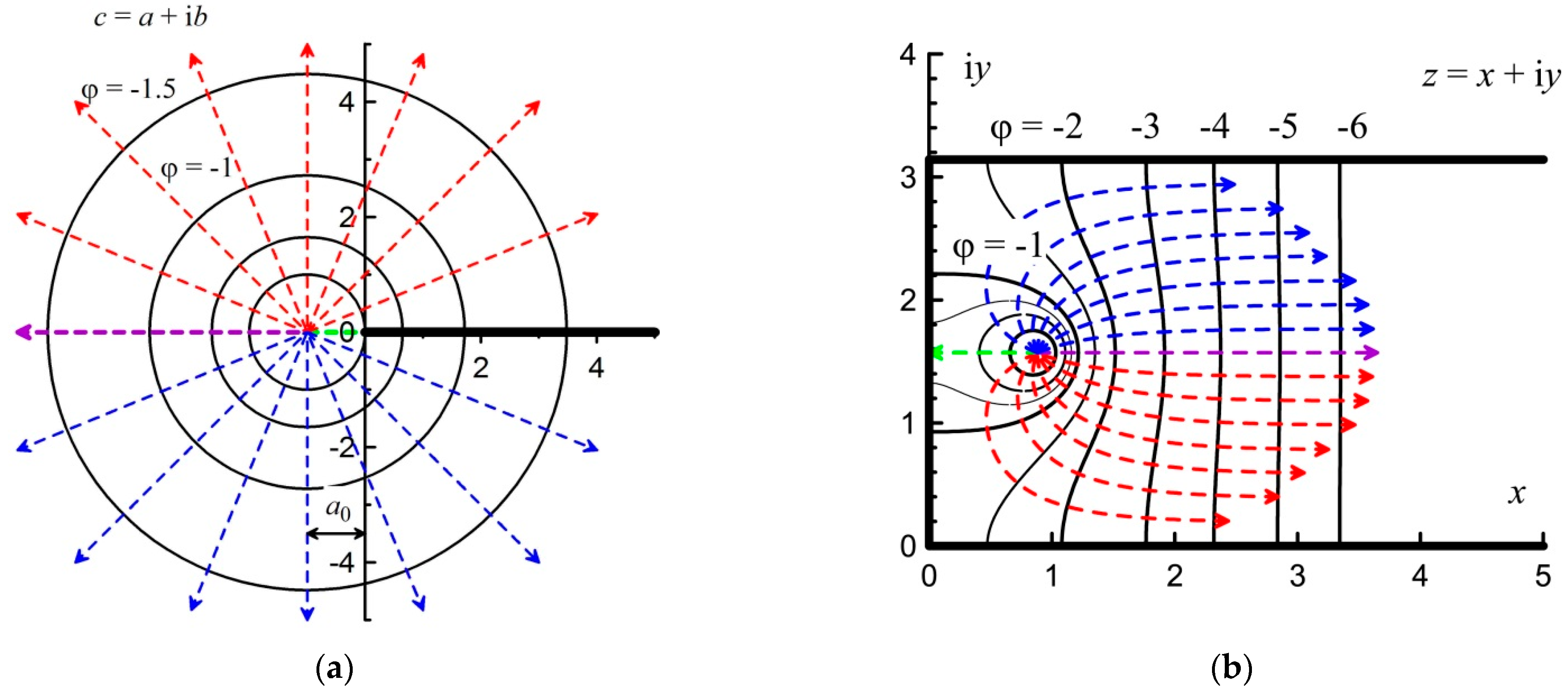
3.1. Axisymmetric Ignition in Unlimited Space

After the axisymmetric ignition in the unlimited two-dimensional complex space c = a + ib, the gas flow can be represented as straight diverging rays, as shown in Figure 3a. Here, i is the imaginary unit.

The direction of flow velocity is represented by dashed straight lines. Red lines indicate upward flow and blue lines indicate downward flow. These straight lines with a slope coefficient k are given by the following equation:

b = ka.

(1)

The purple straight line directed to the left divides the direction of motion. This division by color is made for convenience and the further presentation of the results. The semi-infinite axis in the form of a black line is a thin impermeable wall with zero thickness dividing the space into the upper and lower parts.

For this two-dimensional axisymmetric flow, the velocity of the incompressible fluid (gas) V is inversely proportional to the distance r to the source (inversely proportional to the circumference):

$$V~{\displaystyle \frac{1}{r}}.$$

(2)

In the potential approximation, the flow velocity V is related to the flow potential ϕ by the following equation:

$$\overrightarrow{V}~-\nabla \varphi .$$

(3)

From Equations (2) and (3), we determined that equipotential lines will be represented as circles, the radius of which is related to the potential ϕ by the following equation:

$$r~{\mathrm{e}}^{-\varphi }.$$

(4)

Figure 3a also shows equipotential lines in the form of circles with dimensionless values of potential ϕ = −1; −1.5; −2; −2.5; −3:

$$a^2+b^2=r^2={\mathrm{e}}^{-2\varphi }.$$

(5)

3.2. Semi-Bounded Space

The transition to the unlimited complex space c = a + ib from the semi-bounded space w = u + iv is determined by conformal mapping:

$$c=w^2.$$

(6)

The semi-bounded space w = u + iv is shown in Figure 3b. The direction of the purple beam changed from left to vertical upwards, that is, along the axis of imaginary numbers. The reverse transition from unbounded space to semi-bounded space has the following form:

$$w=c^{{\displaystyle \frac{1}{2}}}.$$

(7)

In this case, the semi-infinite axis turns into an impenetrable wall at the lower boundary of the semi-infinite space. The purple line from the “left” direction turns into the “up” direction. Equipotential circles in this mapping have the form of semicircles. In this case, the radius R of these semicircles decreases: $R~\sqrt{r}$. Accordingly, the modulus of the potential field gradient increases in this case. Therefore, in accordance with Equation (3), the gas flow velocity doubles with the same flow source productivity. The straight lines indicating the flow direction also turn into straight lines. In this case, the direction angle of each ray decreases by half.

3.3. Semi-Bounded Strip: Ignition at the Closed End

The transition to the semi-bounded complex space w = u + iv from the semi-bounded strip z = x + iy is determined by conformal mapping:

$$w=\mathrm{ch}z.$$

(8)

The semi-bounded strip z = x + iy is shown in Figure 4a.

The final transformation from a semi-bounded strip to an unlimited space looks like the following:

$$c={\mathrm{ch}}^{2}z.$$

(9)

The inverse transformation, accordingly, has the following form:

$$z=\mathrm{arcch}\left(c^{{\displaystyle \frac{1}{2}}}\right).$$

(10)

In this case, the impenetrable wall transfers into the lower, upper, and left impenetrable walls of the semi-bounded strip. By substituting the definition of complex variables c = a + ib and z = x + iy into Equation (10), the equations for conformal mapping can be obtained in real variables:

$$a={\displaystyle \frac{1}{2}}\cos 2y\cdot \mathrm{ch}2x+{\displaystyle \frac{1}{2}};\hspace{1em}b={\displaystyle \frac{1}{2}}\sin 2y\cdot \mathrm{sh}2x.$$

(11)

Thus, the equipotential lines from Equation (5) in a semi-bounded strip are given by the following equation:

$${\left({\displaystyle \frac{1}{2}}\cos 2y\cdot \mathrm{ch}2x+{\displaystyle \frac{1}{2}}\right)}^2+{\left({\displaystyle \frac{1}{2}}\sin 2y\cdot \mathrm{sh}2x\right)}^2=r^2=e^{-2\varphi }.$$

(12)

The explicit solution of Equation (12) is presented below in Appendix A. Equipotential lines (12) are shown in Figure 4a by black lines. As can be seen from Figure 4a, the distance between the lines does not change with the distance from the initiation source. This means that the potential gradient is constant, and from Equation (3), it follows that the flow velocity formed at the first stage does not change further.

Similarly, using the transformation Equation (11), new implicit equations can be obtained in a semi-bounded band from the flow line Equation (1):

$${\displaystyle \frac{1}{2}}\sin 2y\cdot \mathrm{sh}2x=k\left({\displaystyle \frac{1}{2}}\cos 2y\cdot \mathrm{ch}2x+{\displaystyle \frac{1}{2}}\right).$$

(13)

These lines are shown in Figure 4a by the dotted red and blue lines. As a result of transformation (13), the purple line from the “up” direction (Figure 3b) goes to the “right” direction. However, the straight lines denoting the direction of flow in other directions acquire a more complex representation. An explicit solution to Equation (13) is given in Appendix A.

The flow rate will be higher in those directions in which the potential changes faster (greater potential gradient, or higher density of potential lines). As can be seen from Figure 4a, the potential changes faster along the strip axis. In other directions, the rate of potential change is lower with a lower modulus of the coefficient K, which characterizes the slope of the straight lines in Figure 3b.

The shape of the flame front can be estimated by the path of combustion products along the trajectory of movement, defined by Equation (13). To determine the velocity W_L of the flow along a certain trajectory L, it is necessary to determine the derivative along this direction:

$$W_{\mathrm{L}}=-{\left({\displaystyle \frac{\partial \varphi }{\partial l}}\right)}_{\mathrm{L}}.$$

(14)

Here, $\partial l$ is the displacement along a trajectory L. Then, the path l′, traveled along the trajectory L in time Δt, is determined by the following equation:

$$l\prime ={\displaystyle \underset{0}{\overset{\Delta t}{\int }}\left|W_{\mathrm{L}}\right|}\mathrm{d}t={\displaystyle \underset{0}{\overset{\Delta t}{\int }}\left|{\left(\frac{\partial \varphi }{\partial l}\right)}_{\mathrm{L}}\right|}\mathrm{d}t.$$

(15)

Integration will allow the shape of the flame front to be determined. Using the equation of the flow lines (13) and the equation of the flow potential (12) it is possible to calculate the integral (15) numerically using the finite difference method. The calculation algorithm is attached in the Supplementary Materials. An assessment of the convergence of this method made it possible to determine the optimal dimensionless spatial step equal to 0.001 and the time interval of 0.001.

In the theoretical model, a centrally symmetric flame front in a small vicinity of the ignition point was considered at the initial stage of ignition. In this case, the flame front shape is close to circular (for ignition at the closed end of the channel, the flame shape is close to semicircular). This assumption corresponds to the actual propagation of the flame front, which has a circular or spherical shape at the initial stage of ignition. Integration and calculation of the flame surface shape starts from this initial position. Figure 4b shows the initial points as black dots, from which integration starts for each of the flow lines. A circle with a dimensionless radius of 0.225 was chosen as a small vicinity of the ignition point, which in this case coincides with a round equipotential surface with a potential of ϕ = +3. Choosing a smaller vicinity inside the round equipotential surface will not lead to a quantitative change in the result.

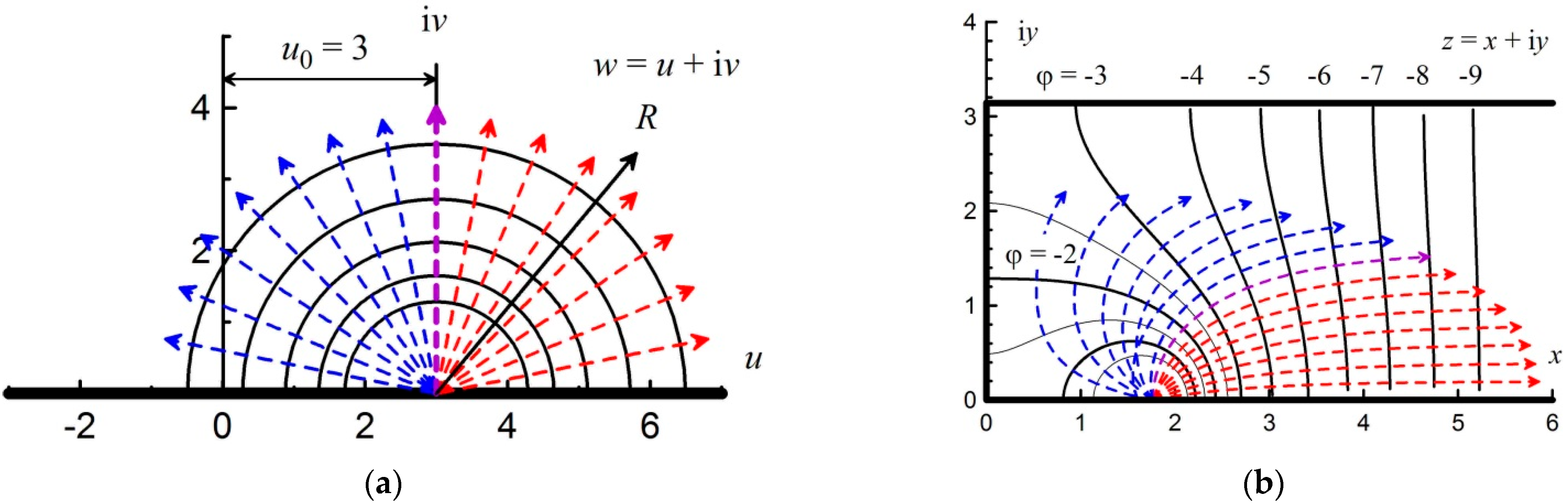
3.4. Semi-Bounded Strip: Ignition on the Axis

In the case of a point ignition at some distance from the closed end of a semi-bounded channel, the source is located on the central purple line, as follows from Figure 4a. This location corresponds to the position of the ignition point in unlimited space to the left at some distance a₀ (a₀ > 0), as shown in Figure 5a. In this case, the equipotential lines and flow lines are given by the following equations:

$${\left(a+a_0\right)}^2+b^2=r^2;$$

(16)

$$b=k\left(a+a_0\right).$$

(17)

The equipotential lines and flow lines for Equations (16) and (17) are shown in Figure 5a by solid and dashed lines, respectively.

Using inverse conformal mapping (10) or the transformation in real variables (11), we can write the equation of equipotential lines and flow lines in a semi-infinite strip:

$${\left({\displaystyle \frac{1}{2}}\cos 2y\cdot \mathrm{ch}2x+{\displaystyle \frac{1}{2}}+a_0\right)}^2+{\left({\displaystyle \frac{1}{2}}\sin 2y\cdot \mathrm{sh}2x\right)}^2=r^2=e^{-2\varphi };$$

(18)

$${\displaystyle \frac{1}{2}}\sin 2y\cdot \mathrm{sh}2x=k\left({\displaystyle \frac{1}{2}}\cos 2y\cdot \mathrm{ch}2x+{\displaystyle \frac{1}{2}}+a_0\right).$$

(19)

Explicit solutions to Equations (18) and (19) are presented in Appendix A. Equipotential lines (18) are also shown in Figure 5b as black lines. Flow lines (19) are shown in Figure 5b as red and blue dashed lines. The figure is given under the condition a₀ = 1. As can be seen from Figure 5b, the potential gradient toward the open end exceeds the gradient toward the closed end. This results in the flow velocity toward the open end exceeding the flow velocity toward the closed end. Unlike ignition at the closed end, when the solution is self-similar, the velocity ratio in this case depends on the position of the source relative to the closed end of the channel.

Using the equation of the flow lines (19) and the equation of the flow potential (18) it is possible to calculate the integral (15) numerically using the finite difference method (attached in the Supplementary Materials). This will make it possible to evaluate the shape of the flame front. At the initial stage of ignition, a circular flame front in a small vicinity of the ignition point was also considered.

3.5. Semi-Bounded Strip: Ignition on the Wall

From Figure 3b, it is evident that the flow structure in a semi-bounded space after ignition at the lower boundary does not change when the ignition point is shifted along this surface. However, looking at Figure 3a and Figure 5a, it can be seen that placing the ignition source on the surface of an impermeable wall can introduce uncertainties in the visual perception and analytical solution. Therefore, it is advisable to limit ourselves to the conformal mapping for this problem (8). Figure 6a shows the corresponding flow map in a semi-bounded space.

When the ignition source is placed to the right at some distance u₀ (u₀ > 0), the equipotential lines and flow lines are given by the following equations:

$${\left(u-u_0\right)}^2+v^2=R^2;$$

(20)

$$v=K\left(u-u_0\right).$$

(21)

Here, K is the slope of the lines in Figure 6a. The equipotential lines and flow lines for Equations (20) and (21) are shown in Figure 6a. Transformation (8) in real variables has the following form:

$$u=\cos y\cdot \mathrm{ch}x;\hspace{1em}v=\sin y\cdot \mathrm{sh}x.$$

(22)

Thus, the equation of equipotential lines and flow lines has the following form:

$${\left(\cos y\cdot \mathrm{ch}x-u_0\right)}^2+{\left(\sin y\cdot \mathrm{sh}x\right)}^2=R^2;$$

(23)

$$\sin y\cdot \mathrm{sh}x=K\left(\cos y\cdot \mathrm{ch}x-u_0\right).$$

(24)

Explicit solutions to Equations (23) and (24) are presented in Appendix A. Equipotential lines (23) are also shown in Figure 6b as black lines. Flow lines (24) are shown in Figure 6b as red and blue dotted lines. As can be seen from Figure 6b, the potential change is greatest toward the open end. This results in the flow velocity toward the open end exceeding the flow velocity toward the closed end.

Using the equation of the flow lines (24) and the equation of the flow potential (23) it is possible to calculate the integral (15) numerically using the finite difference method (attached in the Supplementary Materials). At the initial stage of ignition, a semicircular flame front was considered in a small vicinity of the ignition point.

4. Experimental and Theoretical Results

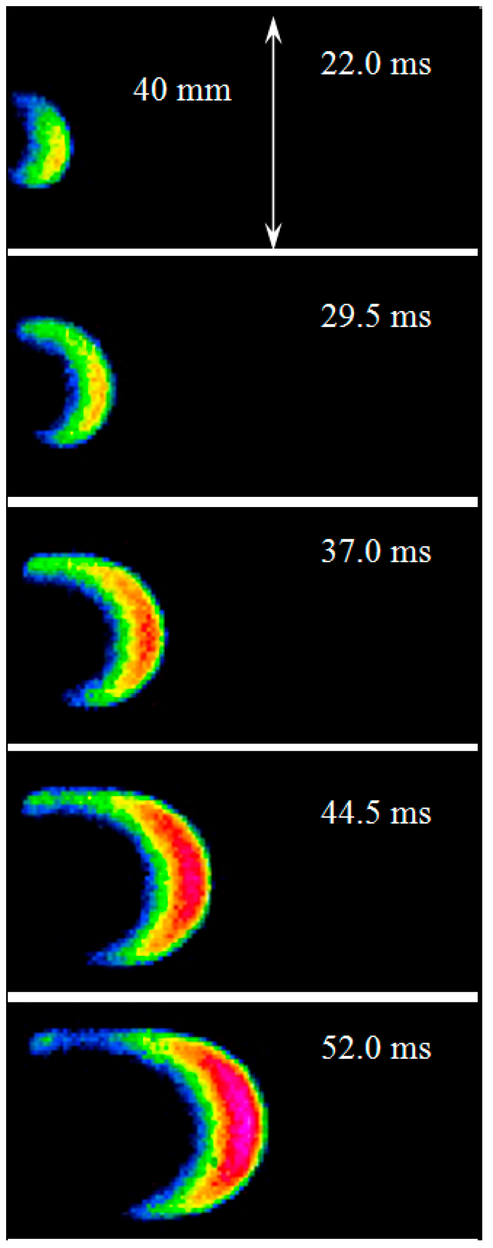
4.1. Ignition at the Closed End of the Channel

Figure 7 shows typical images of the finger flame obtained for a hydrogen–air mixture (11% vol.) at an initial mixture pressure of 40 kPa. The presented flame front shape is called a finger flame. In this case, at the specified mixture pressures and hydrogen concentrations, the flame front was unperturbed. The average flame front velocity in this area was about 1.2 m/s, which was comparable to the calculated flame front velocity value of 1.11 m/s, equal to the laminar velocity of 0.3 m/s [34,35] multiplied by the combustion product expansion ratio of 3.7 [36].

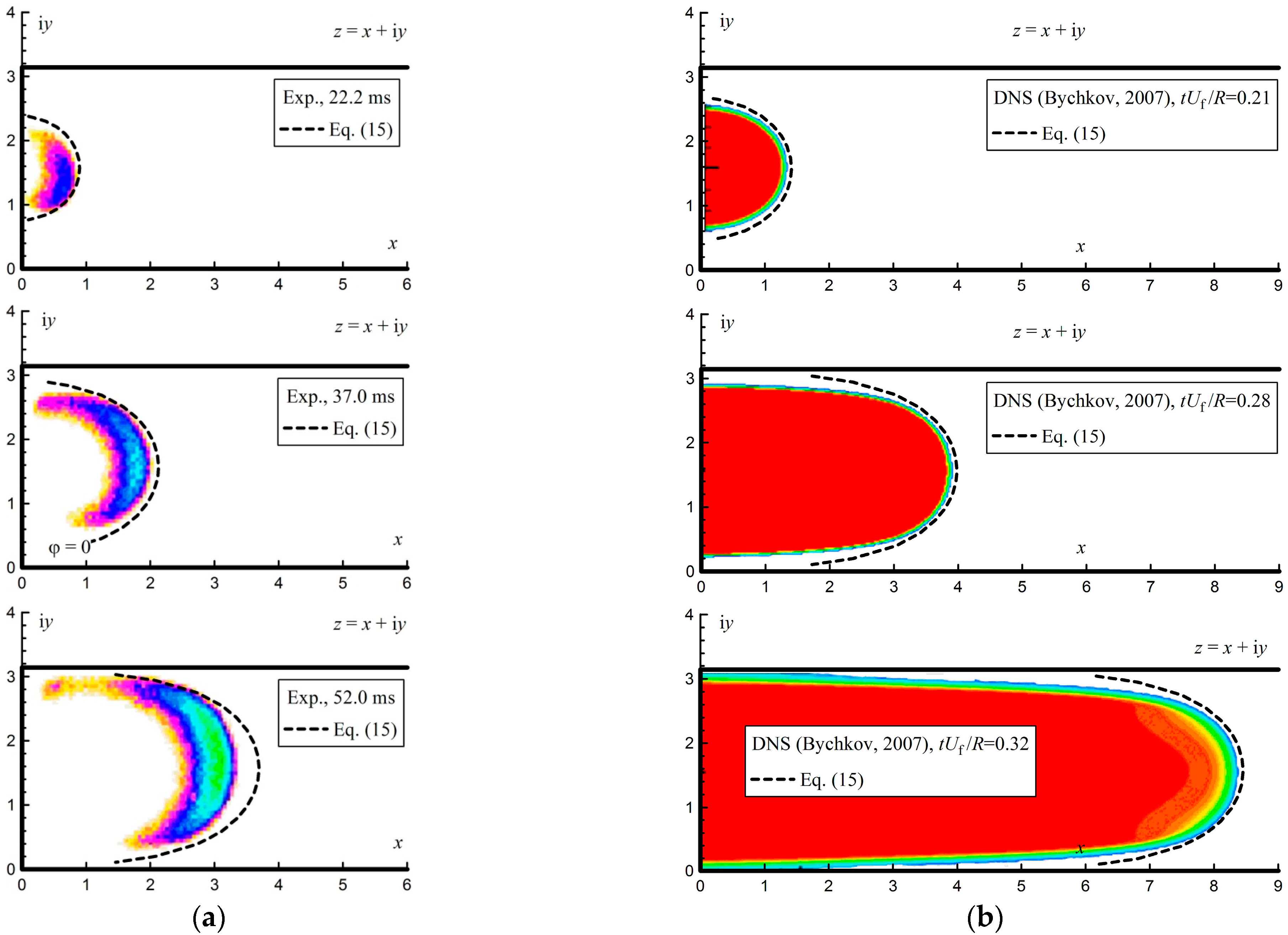
Figure 8a shows the results of integrating Equation (15) for the fifteen trajectories shown in Figure 4. At the same time, the images from Figure 7 are shown, inverted in color for better perception. As can be seen from Figure 8a, the analytical shape of the flame front agrees with the shape determined experimentally. Significant differences in the flame shape were observed with an increasing registration time after the ignition. The calculated curve takes a more elongated shape. This is due to the fact that the analytical solution does not take into account the diffusion processes that occur with strong curvatures of the flow lines and that determine the transfer of heat and the displacement of reagents between the flow lines.

Figure 8b shows the results of a comparison of the analytical solution with the results of numerical modeling obtained using the direct numerical simulations method (DNS) [37]. The method in Ref. [37] employs a global Arrhenius model with parameters, such as the thermal expansion ratio, chosen to be representative for stoichiometric propane-air mixtures (thermal expansion ratio θ = 8). As can be seen, the analytical shape of the flame front was less elongated in this case compared to the calculated results. Thus, the conformal mapping of an unlimited space into a semi-limited strip allows us to estimate the structure of the flow of the unburned mixture in front of the flame front.

4.2. Ignition at the Axis of the Channel

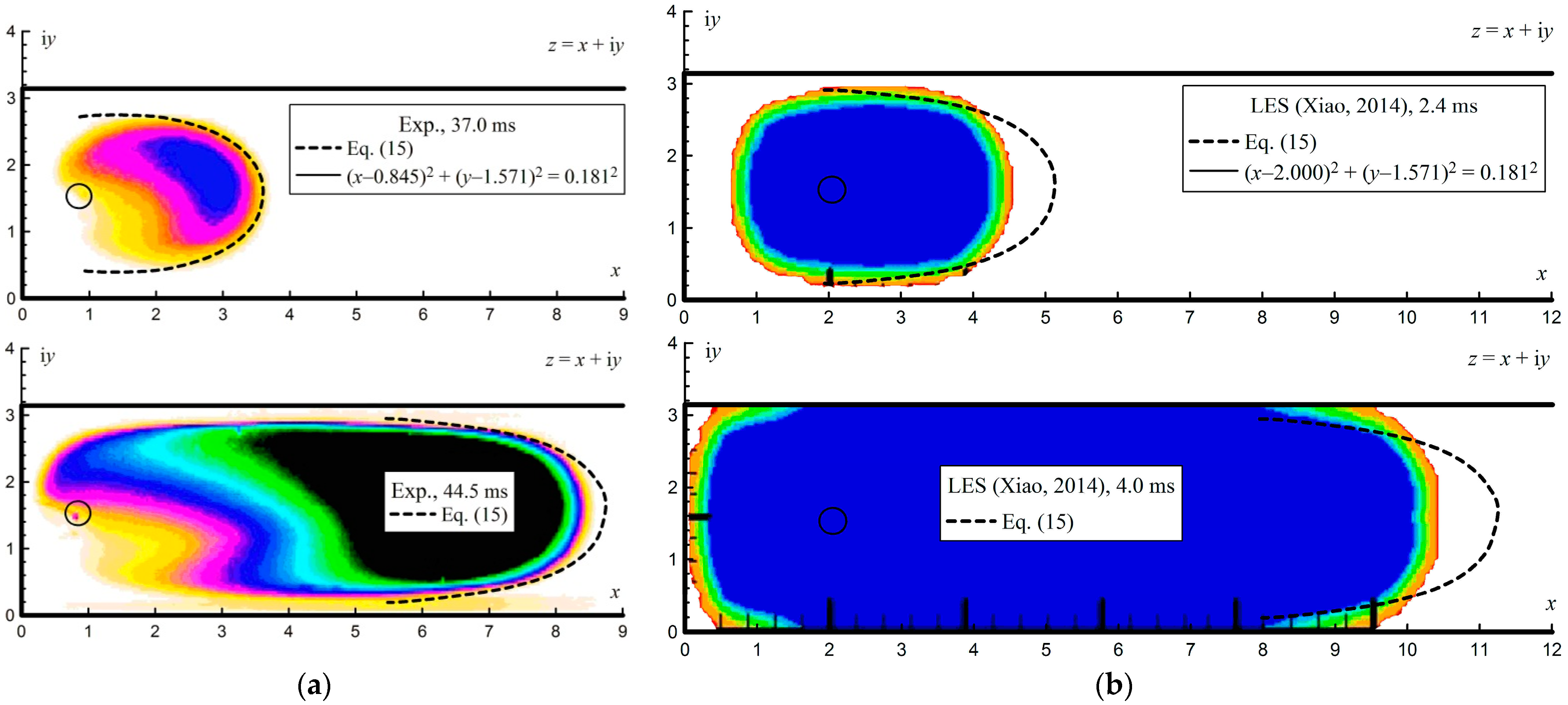
Figure 9 shows typical images of the undisturbed finger flame obtained for an acetylene–air mixture (6.3% vol.) at an initial pressure of 30 kPa. The average flame front velocity increased from 1 m/s (between 0 ms and 7.5 ms) to 10 m/s (between 37.0 ms and 44.5 ms). This velocity is also comparable to the laminar combustion velocity of 1.1 m/s [38] multiplied by the expansion ratio of the combustion products of 7.64 [39], equal to 8.4 m/s. The obtained images were also compared with the results of the analytical assessments.

Figure 10a shows the results of the analysis with a dotted line. For the experimentally established position of the ignition source in space z = x + iy, the coordinates of its image in unlimited space c = a + ib were determined using Equation (11). Then, using Equations (18) and (19), the flow trajectories were determined. The initial shape of the flame front was specified by a circle in a small vicinity of the ignition point by the equation (x − 0.845)² + (y − 1.571)² = 0.181². As in the case of ignition at the closed end of the channel, the integration and calculation of the flame surface shape starts from this initial circular position. This circle was closed to the equipotential surface with a potential of ϕ = 0.

Figure 10a also shows the experimental results presented earlier in Figure 9 for comparison. The images are inverted in color for better perception. As can be seen from Figure 10a, the evaluated flame shape coincides with the experimentally obtained flame shape. However, it is worth noting that, as the flame front moves away from the ignition point, the analytical curve begins to stretch. As noted, this may be due to the fact that the model does not take into account the transfer processes between flow lines.

Figure 10b shows the results of a comparison of the analytical solution with the results of numerical modeling obtained using the large eddy simulation method (LES) [40]. As can be seen, the analytical shape of the flame front in this case was also more elongated compared to the calculated results. A similar pattern was also observed when comparing with the numerical results in [41,42], for which the CABARET method was used.

In this case, the conformal mapping of the unlimited space into a semi-bounded strip also allowed us to estimate the structure of the flow of the unburned mixture upon ignition on the channel axis. However, the analytical estimates yielded a coincidence at a distance of two channel calibers. At a greater length, the analytical flame shape began to stretch out compared to the experimental or calculated one.

4.3. Ignition at the Wall of the Channel

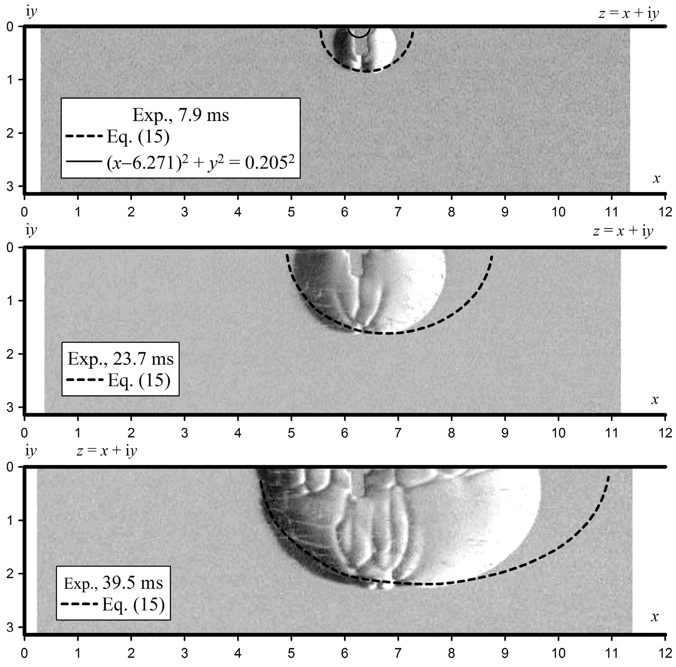
Figure 11 shows typical schlieren images of the flame obtained for a hydrogen–air mixture (30% vol.) at an initial pressure of 100 kPa during ignition on the side wall of the channel. The values of the flame front velocities in three directions are presented in detail in [33].

Figure 11 shows also the results of the analysis with a dotted line. The initial shape of the flame front was given by a semicircle in a small vicinity of the ignition point by the equation (x − 6.271)² + y² = 0.205². Integration and calculation of the flame surface shape starts from this initial position. This circle was closed to the equipotential surface with a potential of ϕ = 0. As can be seen from Figure 11, the evaluated flame shape coincided qualitatively with the experimentally obtained flame shape. However, it is worth noting that, as the flame front moved away from the ignition point, the analytical curve began to stretch.

4.4. Formation of a Tulip Flame in the Potential Approximation

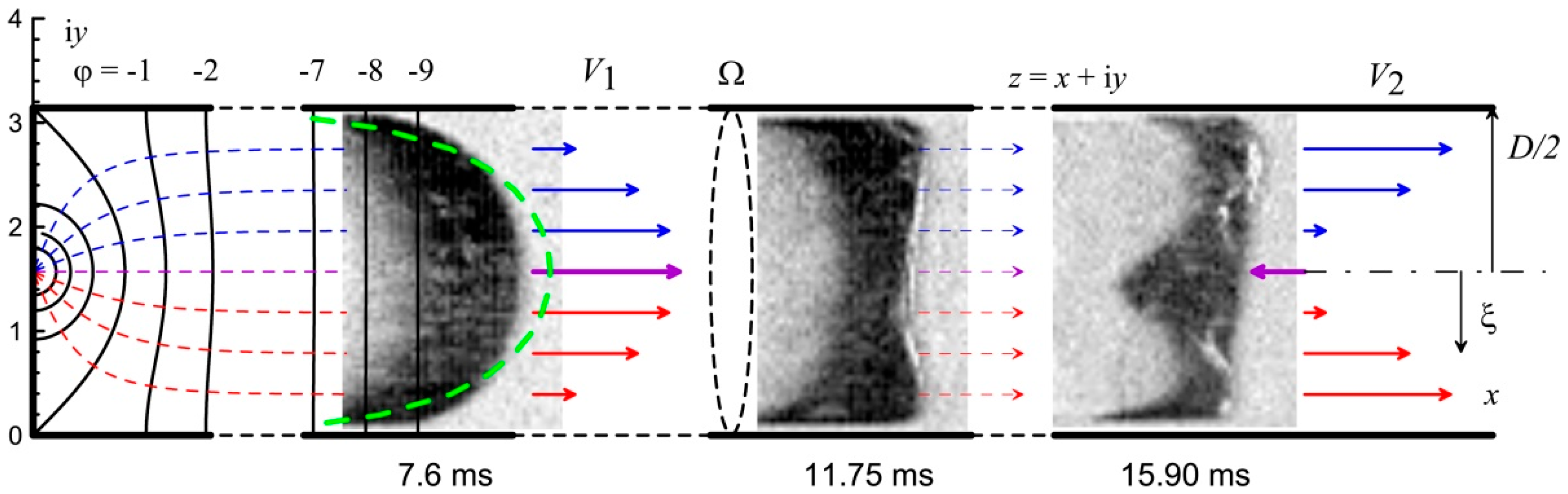
Figure 12 shows typical images of the transition of a finger flame to a tulip-shaped flame obtained for an acetylene–air mixture (7.8% vol.) at an initial pressure of 100 kPa. As can be seen from the figure, at the moment of time 7.60 ms after ignition, a finger flame is registered. And between 11.75 ms and 15.90 ms, the finger flame transitions to a tulip flame. At the same time, the average velocity of the most distant point on the flame front decreases from 2.7 m/s to 1.7 m/s.

As follows from Figure 4a, the velocity distribution along the channel axis during the propagation of the finger flame was non-uniform. The flow velocity of the unburned mixture was at the maximum at the channel axis and at the minimum at the walls. Moreover, for a real flow, the velocity on the side wall tended to zero due to viscous effects. The velocity V₁ of the flow is shown schematically in Figure 13 for a time of 7.6 ms. Figure 13 also displays the results of the analysis using a green dotted line. As can be seen from the figure, the theoretical flame shape is slightly more elongated than that of the experimental shape.

As noted above, the propagation of the flame front is determined not only by the flow of the unburned mixture, but also by the processes of reagent diffusion, thermal diffusion, and heat transfer. Therefore, with significant curvatures of the flame front surface, especially when approaching the channel walls, the flame front propagates toward the channel walls, reaching them in a finite time interval. After this, combustion occupies the entire cross-section of the channel. In this case, the flow near the walls will be determined not by the initial axisymmetric expansion of the combustion products, but by the newly formed flow of the combustion products expanding along the channel axis over its entire cross-section, as shown in Figure 13 at 11.75 ms. The axial velocity of the unburned mixture flow near the channel walls, determined by the combustion of the mixture near the channel walls, will be numerically close to the velocity of the unburned mixture on the channel axis. The expected distribution of longitudinal velocities will tend to a uniform distribution.

However, in this case, the distribution of equipotential lines will change. Since the new flow does not correspond to the initial formulation of axisymmetric ignition, the transition to a new potential distribution will occur abruptly. However, the flow continuity equation will not allow an abrupt increase in the flow velocity of the unburned mixture over the entire cross-section of the channel. The total flow rate Q is determined by the following equation:

$$Q={\displaystyle \underset{\Omega }{\int }\rho \left(\overrightarrow{V}\mathrm{d}\overrightarrow{S}\right)}.$$

(25)

Here, Ω is the cross-section of the channel, ρ is the gas density, and $\overrightarrow{V}$ is the velocity of the gas flowing through the area element dS on the surface Ω. In the case where the flame front velocity is significantly lower than the sound speed and in the isobaric approximation (density ρ = const for the unburned mixture), Equation (25) can be rewritten for a narrow channel:

$$2\rho h{\displaystyle \underset{0}{\overset{D/2}{\int }}{V}_1^{\mathrm{axis}}\left(\xi \right)\mathrm{d}\xi }=2\rho h{\displaystyle \underset{0}{\overset{D/2}{\int }}{V}_2^{\mathrm{axis}}\left(\xi \right)\mathrm{d}\xi }.$$

(26)

Here, h is the channel height, D is the channel width (h << D), and $V_1^{\mathrm{axis}}\left(\xi \right)$ and $V_2^{\mathrm{axis}}\left(\xi \right)$ are the distributions of the axial velocities of the unburned mixture over the channel cross-section before the flame front touches the channel walls and after touching. It follows from Equation (26) that an increase in the velocity at the channel walls (ξ → D/2) will inevitably lead to a decrease in the velocity at the channel axis (ξ → 0). In this case, the velocity at the channel axis can have a negative value. This effect of velocity reversal at the channel axis will be especially pronounced for channels with a larger cross-section. For example, for a channel with a circular cross-section, Equation (24) can be rewritten as follows:

$$2\pi \rho {\displaystyle \underset{0}{\overset{D/2}{\int }}{V}_1^{\mathrm{axis}}\left(\xi \right)\xi \mathrm{d}\xi }=2\pi \rho {\displaystyle \underset{0}{\overset{D/2}{\int }}{V}_2^{\mathrm{axis}}\left(\xi \right)\xi \mathrm{d}\xi }.$$

(27)

As can be seen from Equation (27), the further the registration point |ξ| is from the channel axis, the greater its contribution to the increase in flow velocity. In this case, the velocity at the channel axis can have a negative value, as can be seen in Figure 13 at time 15.90 ms.

When considering Equations (26) and (27), it should be taken into account that the flow is laminar. In this case, there should be no disturbances on the flame front. The formation of a disturbed tulip-shaped flame will require additional conditions that are quite difficult to take into account in a potential flow.

5. Discussion

As the results showed, conformal mapping enables the description of changes in the flame front shape in the channel at the initial stage of ignition. By comparing the obtained results with our experimental results and the results of published numerical studies, it can be concluded that the conformal mapping allows for a fairly quick assessment of the flow structure without taking into account the chemistry of the combustion process. The presented method can be used to test numerical algorithms at the initial stage of ignition.

It is worth noting that this method has its drawbacks. For example, the presented method does not take into account the transfer processes between the flow layers, so it will not be adequate for large time intervals. In addition, this method does not take into account instabilities, because such a method does not assume their presence.

The considered model of the potential flow of finger flame, as well as transition to tulip flame, implies the absence of compression waves both at the moment of initiation and at initial acceleration of the flame front. Reflection of the waves from the walls of the channel can lead to disturbance of the flame front. Therefore, in the analysis it is necessary that the initiation energy be significantly less than the energy of direct initiation of detonation. In this case, the value of the initiation energy does not appear in the analysis.

The proposed method does not consider a specific reactive mixture. The only parameter that can affect the change in the flame front shape in dimensionless coordinates is the thermal expansion ratio of the combustion products. The contribution of the thermal expansion ratio θ in a small displacement dl′ of the trajectory L in Equation (15) will lead to an increase in the displacement of the combustion products: $\mathrm{d}{\mathrm{l}}^{\prime }=\left|{\mathrm{W}}_{\mathrm{L}}\right|\mathrm{d}\mathrm{t}$. The constant θ is the same for all trajectories L. Thus, a change in the thermal expansion ratio of the combustion products can affect the velocity of flame front propagation but cannot affect the shape of the flame front at each specific position inside the channel. The thermal expansion ratio will have a significant effect only at large distances when approaching the walls, i.e., at distances of the head point more than two calibers. In this case, the combustion products will expand not only along the trajectory, but also between the trajectories.

6. Conclusions

Based on the results of the theoretical evaluations, it can be concluded that the use of conformal mappings can help to estimate the flow of the unburned mixture and the flame front dynamics after an ignition point.

Conformal mapping allows the flow structure to be estimated for a finger flame, an elongated flame when ignited at the channel axis or at the channel wall. A comparison of the analysis with images of the flame front showed a qualitative agreement between the theoretical analysis and the experimental data or numerical data.

It is worth noting that the propagation of the flame front is determined not only by the flow of the unburned mixture caused by the expansion of combustion products, but also by the processes of diffusion of reagents, thermal diffusion, and heat transfer. With the strong curvatures of the flame front, especially when approaching the channel walls, the direction of movement of the flame front may differ from the direction of displacement of this mixture relative to the channel walls. Therefore, at distances greater than two calibers from the ignition point, the analytical shape of the flame front is stretched out in comparison with the experimental or numerical results. Moreover, the subsequent application of potential flow may lead to flow deviations and an incorrect representation of the flame shape. These conditions distinguish the study of the dynamics of reacting systems from the dynamics of inert gases and liquids.