Article

Data-Driven Health Status Assessment of Fire Protection IoT Devices in Converter Stations

1
State Grid Anhui Electric Power Research Institute, Hefei 230001, China
2
State Grid Laboratory of Fire Protection for Transmission and Distribution Facilities, Hefei 230031, China
3
Anhui Provincial Key Laboratory of New Type Power Systems Fire Safety and Emergency Technology, Hefei 230061, China
4
State Key Laboratory of Fire Science, University of Science and Technology of China, Hefei 230027, China
5
Advanced Technology Research Institute, University of Science and Technology of China, Hefei 230026, China
*
Authors to whom correspondence should be addressed.
Fire 2025, 8(7), 251; https://doi.org/10.3390/fire8070251
Submission received: 11 May 2025 / Revised: 18 June 2025 / Accepted: 25 June 2025 / Published: 27 June 2025

Abstract

To enhance fire safety in converter stations, this study focuses on detecting abnormal data and potential faults in fire protection Internet of Things (IoT) devices, which are networked sensors monitoring parameters such as temperature, smoke, and water tank levels. A data quality evaluation model is proposed, covering both validity and timeliness. For validity assessment, a transformer-based time series reconstruction method is used, and anomaly thresholds are determined using the peaks over threshold (POT) approach from extreme value theory. The experimental results show that this method identifies anomalies in fire telemetry data more accurately than traditional models. Based on the objective evaluation method and clustering, an interpretable health assessment model is developed. Compared with conventional distance-based approaches, the proposed method better captures differences between features and more effectively evaluates the reliability of fire protection systems. This work contributes to improving early fire risk detection and building more reliable fire monitoring and emergency response systems.

1. Introduction

With the development of the Internet of Things (IoT), an increasing number of intelligent fire protection sensors have been deployed in various fire-risk scenarios. However, due to factors such as aging, electromagnetic interference, and external damage, the data quality and health status of these sensors may degrade over time. Therefore, it is essential to evaluate the data quality and health status of fire protection IoT devices, enabling the early identification of performance degradation. This helps in maintaining control over critical monitoring variables during fire detection and firefighting decision-making, thereby reducing casualties and property loss.
The current research on data quality assessment primarily focuses on two aspects: anomaly detection and data quality evaluation. The former aims to determine whether individual time series are anomalous, while the latter seeks to quantitatively evaluate the overall quality of the data. In terms of anomaly detection, existing studies fall into two main categories: statistical methods and artificial intelligence approaches. For instance, Bianco [1] developed an autoregressive moving average model to detect errors and identify outliers; Garcia [2] applied multivariate statistical process control to identify offset and drift anomalies in bridge monitoring data; and Samparthi et al. [3] proposed an anomaly detection model for sensor data streams based on kernel density estimation. Among AI-based methods, Gu Yaxiong [4] employed the K-nearest neighbors algorithm to diagnose data validity and used the C4.5 algorithm to analyze the support from neighboring sensors for target sensors, thereby evaluating data effectiveness. Arias et al. [5] introduced a non-parametric anomaly detection algorithm that combines isolation mechanisms with distance-based analysis. Wu Di [6] proposed a supervised learning method based on convolutional neural networks (CNNs) to identify anomalous data in bridge health monitoring by transforming time series into visual images. Hooshmand et al. [7] applied the t-SNE technique for feature visualization to cluster data into different protocol categories, and employed one-dimensional convolutional networks to independently process and classify network traffic anomalies within each category. Audibert et al. [8] proposed a method named USAD, which combines autoencoders and generative adversarial networks (GANs). This approach compresses data into low-dimensional representations using autoencoders and leverages adversarial training to amplify reconstruction errors, thereby isolating anomalies. Gao [9] combined unsupervised learning with anomaly labels using a stacked autoencoder to detect anomalies in oil quality time series (e.g., density, viscosity, and temperature). Darban et al. [10] introduced a contrastive learning approach in which normal samples are transformed into synthetic anomalies using generative methods to serve as negative samples, enabling time series anomaly detection.
In the area of data quality assessment, most methods rely on subjective evaluation by analyzing features such as integrity, outliers, uniqueness, and accuracy to detect duplicate, erroneous, or missing data elements, ensuring data compliance and feedback [11,12,13,14,15]. However, existing comprehensive data quality evaluation methods are limited, as they typically rely on simple threshold-based judgments and fail to capture the dynamic characteristics of time series. Thus, integrating deep learning-based anomaly detection into comprehensive data quality assessment systems is both necessary and promising.
Health status assessment of equipment in the field of fault detection and diagnosis mainly focuses on detecting faults and assessing their severity. Such technologies have been widely applied in various domains, including bearings [16], wind turbines [17], aircraft engines [18], cutting tools, gas turbines [19], and in-orbit satellites [20]. Fault diagnosis methods can generally be classified into manual diagnosis, analytical modeling, signal processing, and machine/deep learning. Manual diagnosis relies on on-site expertise; analytical modeling requires the establishment of accurate mathematical models for each system. Signal processing methods, for example, that reported by Hao et al. [21], analyzed different fault types in high/medium pressure gas regulators through online safety monitoring and provided corresponding alarm rules. Gao Fan et al. [22] constructed a knowledge base and fault tree to extract diagnostic rules and compared FFT spectra from motor drive ends with the rules to assess the health status and fault types of centrifugal pumps. However, signal-based diagnostic methods are significantly affected by background noise and rely heavily on empirical analysis, which limits their reliability for real-time fault diagnosis [23]. In the field of fault diagnosis based on machine learning and deep learning, Aker et al. [24] combined discrete wavelet transform with a naïve Bayes classifier to detect and classify faults in transmission lines; meanwhile, Choudhary et al. [25] integrated thermal imaging with convolutional neural networks to achieve non-contact bearing fault diagnosis.
In recent years, some deep learning models have been applied to fault detection in fire protection equipment. For instance, Zhao Jiahao [26] combined a variational autoencoder (VAE) with a gated recurrent unit (GRU) to reconstruct and predict data, calculating the Euclidean distance between predicted and actual values in the next time window to detect carbon monoxide sensor anomalies. Sousa et al. [27] extracted 22 features (such as peak value, skewness, and mean) from normal smoke sensor operation data and used an autoencoder to reconstruct features. A predefined reconstruction error threshold was then used to detect sensor faults, enabling early detection before scheduled maintenance or sensor replacement.
Currently, temporal reconstruction-based data anomaly detection models face two primary limitations. First, their large parameter size and high computational complexity pose challenges for practical deployment. Second, while validation typically relies on public datasets, these datasets generally lack time-series data relevant to the Fire Internet of Things (Fire IoT), making it difficult to adequately verify the models’ generalization capability in this domain. Regarding equipment health assessment, existing approaches predominantly focus on binary classification of fault occurrence, with insufficient quantitative characterization of fault severity. Although deep learning methods, such as autoencoders, can provide quantitative metrics through reconstruction error (where larger errors usually indicate a higher probability of fault or greater severity), these models inherently lack intuitive interpretability and often exhibit inconsistent results across training runs. Therefore, the author combines subjective and objective evaluation methods and artificial intelligence, using the transformer neural network model to identify the validity of the data, combined with the timeliness of the data to obtain the comprehensive quality of the data. Based on the quality of the data, using the clustering method to identify the fault samples, with the subjective and objective weights to obtain the degree of abnormality index representing the state of health of the equipment, a quantitative measure of the degree of deviation of the equipment from the normal operation of the method, this method has a high data anomaly recognition rate and high fault degree interpretability.

2. Methods

The overall flow of this converter station fire IOT equipment health status assessment is shown in Figure 1.

2.1. Comprehensive Quality Assessment Model for IoT Data

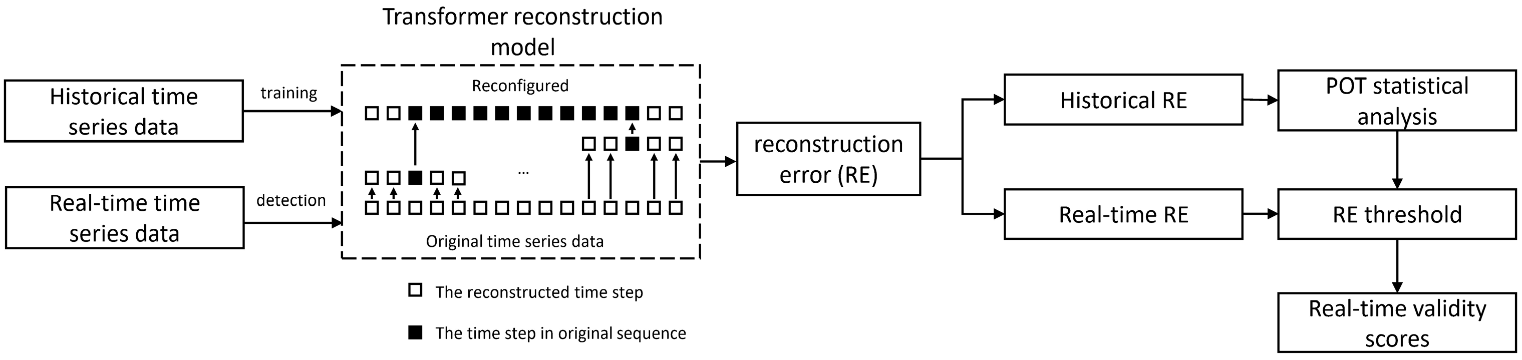
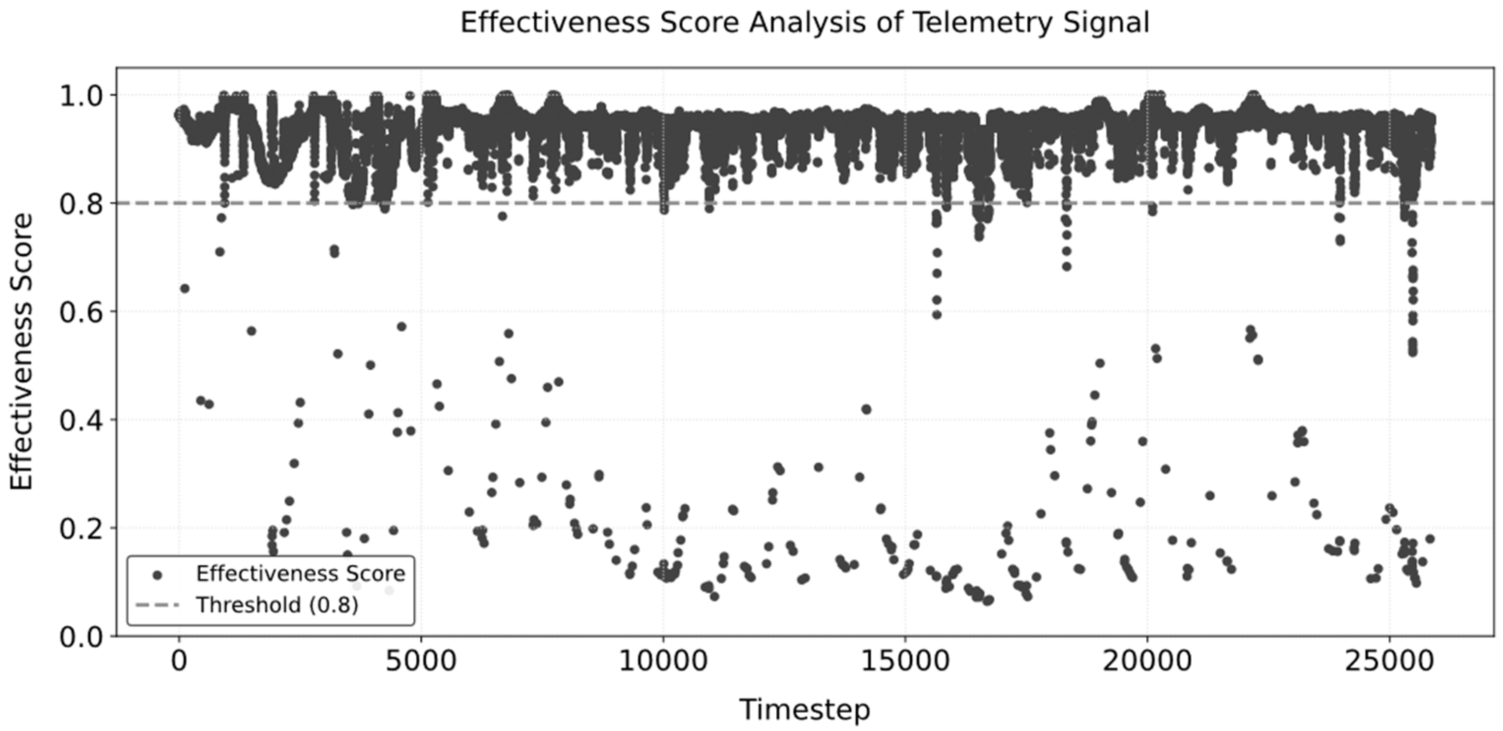
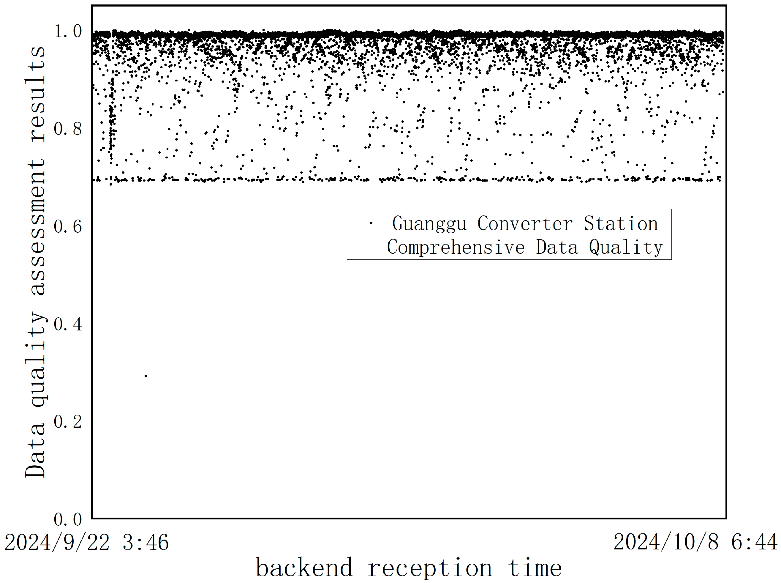
2.1.1. Data Validity Assessment

The validity assessment of telemetry data is based on the pre- and post-relationship of data, and for supervised learning, it is difficult to measure the degree of abnormality of individual time-step data, while unsupervised methods, such as reconstruction and prediction, can determine whether an abnormality occurs in the time-step and combine with the threshold selection method to obtain the quantitative expression of the degree of abnormality.
The effectiveness evaluation adopts the evaluation method based on time series reconstruction, the model used is the transformer reconstruction model, and the automatic threshold acquisition method is the threshold acquisition method based on the POT extreme value theory; the overall process is shown in Figure 2.
As can be seen in Figure 2, the output of the transformer model is single time-step data, and the inputs of the model are the before and after time-series data of the desired reconstructed data, where the input sequence before the reconstructed sequence has a length of L i , and the input sequence after the reconstructed sequence has a length of L i + , is set to L i = L i + = N . The advantage of such a setting is that it allows the network to fully learn the pattern of change before and after the data. For this input sample data set time step length, the number of features is 2. That is, before and after the reconstruction sequence time series data, training set construction used the original time series sliding window, and the number of samples is determined by the original time series length.
In terms of transformer model structure, the reconfiguration model network structure is shown in Figure 3:
As shown in Figure 3, the input data are first dimensionally expanded by a linear layer, and positional encoding is added to enhance the model’s ability to perceive temporal information. The core of the model consists of the transformer encoder, which contains multi-head self-attention, feed-forward network (FFN), and residual connection and layer normalization to ensure training stability and feature normalization.
The core innovation of the transformer is its attention mechanism, which abandons the sequence recursion structure of traditional RNNs and instead dynamically models the dependencies between arbitrary positions in the input sequence through self-attention. Specifically, the mechanism computes the attention weights between all time steps through the matrix operation of query, key, and value to aggregate the global context information. This design not only solves the long-range dependency problem, but also supports parallel computation, which significantly improves the performance of the model in tasks such as machine translation and text generation.
As it is a single-time-step reconstruction task, it is not necessary to combine the decoder part of the Transformer, and using only the encoder reduces the computational overhead while maintaining the performance and reduces the hardware performance and training time required for training.
As shown in Figure 2, the original time series data are preprocessed and input into the deep learning model, and finally, the reconstructed time series is output, which is compared with the original time series to obtain the reconstruction relative error of each time step in order to allow combination into a new reconstruction error time series. Unsupervised temporal anomaly detection argues that time steps with larger reconstruction errors are more likely to be anomalous because they are more likely to deviate from the intrinsic laws of the temporal sequence learned by deep learning, and thus various types of statistically based reconstruction error threshold acquisition methods are applied to unsupervised anomaly detection.
This validity assessment uses the POT automatic selection method, POT (peaks-over-threshold) is a threshold automatic selection method based on extreme value theory. The theory holds that different things may differ in data distribution, but their extreme events will mathematically show a consistent distribution, i.e., the portion of their extreme values exceeding a certain threshold conforms to the Pareto distribution. And the extreme values are usually located in the tails of the probability distribution; the basic idea of the POT algorithm is to fit the tails of the probability distribution through the generalized Pareto distribution with parameters. The formula is shown below:
F ¯ s = P S t h > s | S > t h ~ 1 + γ s β 1 γ
where S = { S 1 , S 2 , , S N } represents the anomaly score calculated for the time-series data with N feature dimensions. The anomaly score also has N dimensions, with each dimension corresponding to the respective feature. t h represents the initial threshold for the anomaly score, and S t h represents the portion of the score that exceeds the threshold. γ and β are the shape and scale parameters of the generalized Pareto distribution, respectively. Both parameters are estimated using the maximum likelihood estimation method. And the final threshold t h F is calculated using the following formula:
t h F t h β ^ γ ^ q N N t h γ ^ 1  
where q represents the expected probability of observing S > t h , N is the number of feature dimensions for the anomaly score S , and N t h is the number of feature dimensions that satisfy the condition S i < t h .
After obtaining the historical statistical data of the reconstruction error, the POT extreme value theory method is used to determine the reconstruction error threshold. Real-time data with reconstruction errors greater than the threshold are identified as anomalous data. Additionally, based on this threshold, a data validity evaluation function can be designed, which satisfies the following requirements:
e i = 0 , δ i = 1 e i , δ i 0 e i = ε , δ i = δ l
where e i is the relative reconstruction error at the time step, ε is the anomaly threshold automatically obtained for each time series using the method mentioned above, δ i is the validity score at time step i , and δ l is the validity score set for telemetry data when the relative error at a time step is judged to be anomalous. To satisfy the above requirements, the specific form of the function can be expressed as follows:
δ i = 2 2 1 + e β e i
where β = ln δ l / 2 δ l ε . By setting the validity score for telemetry data when judged to be anomalous, the validity evaluation result for each time step can be obtained through δ i .

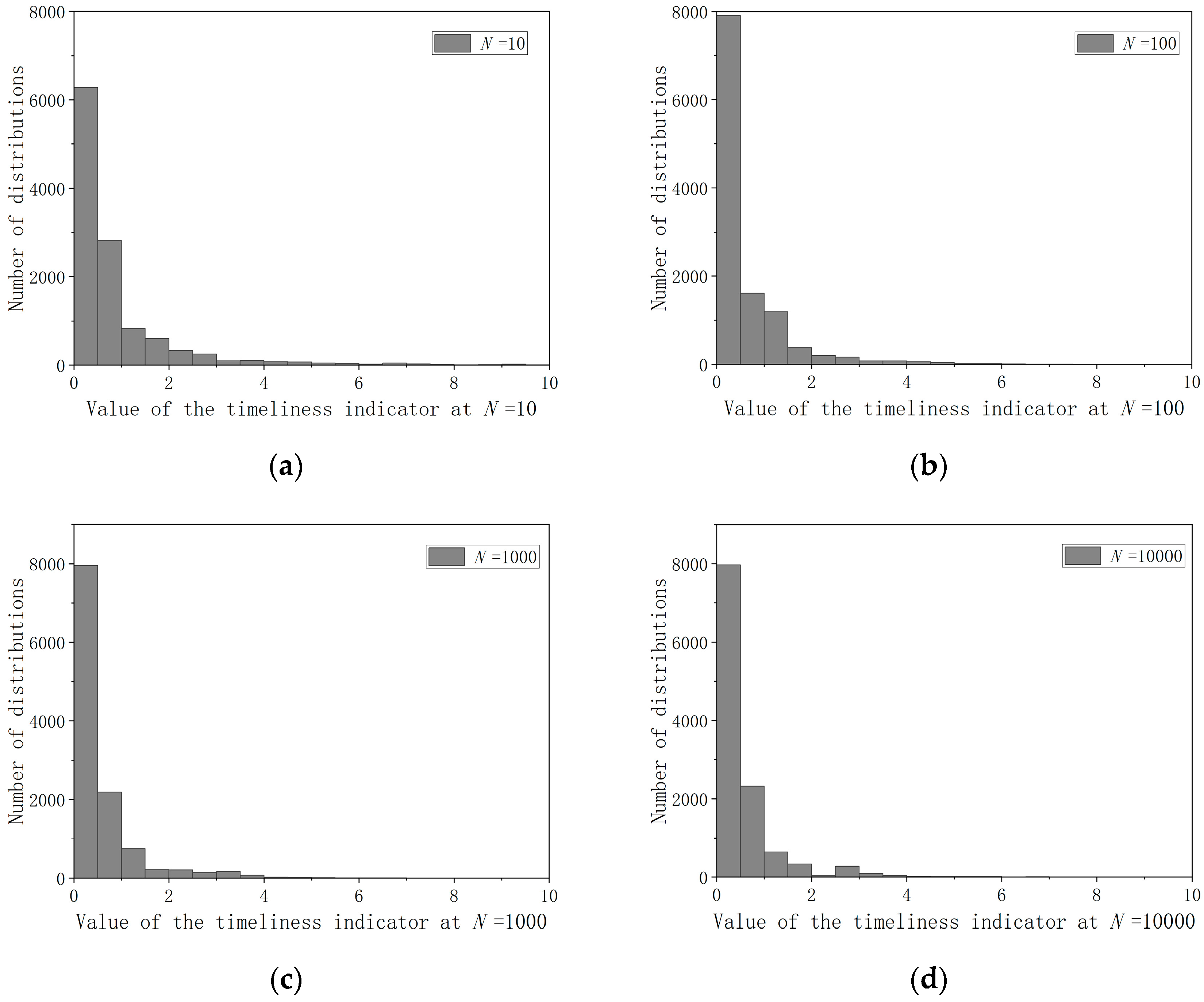
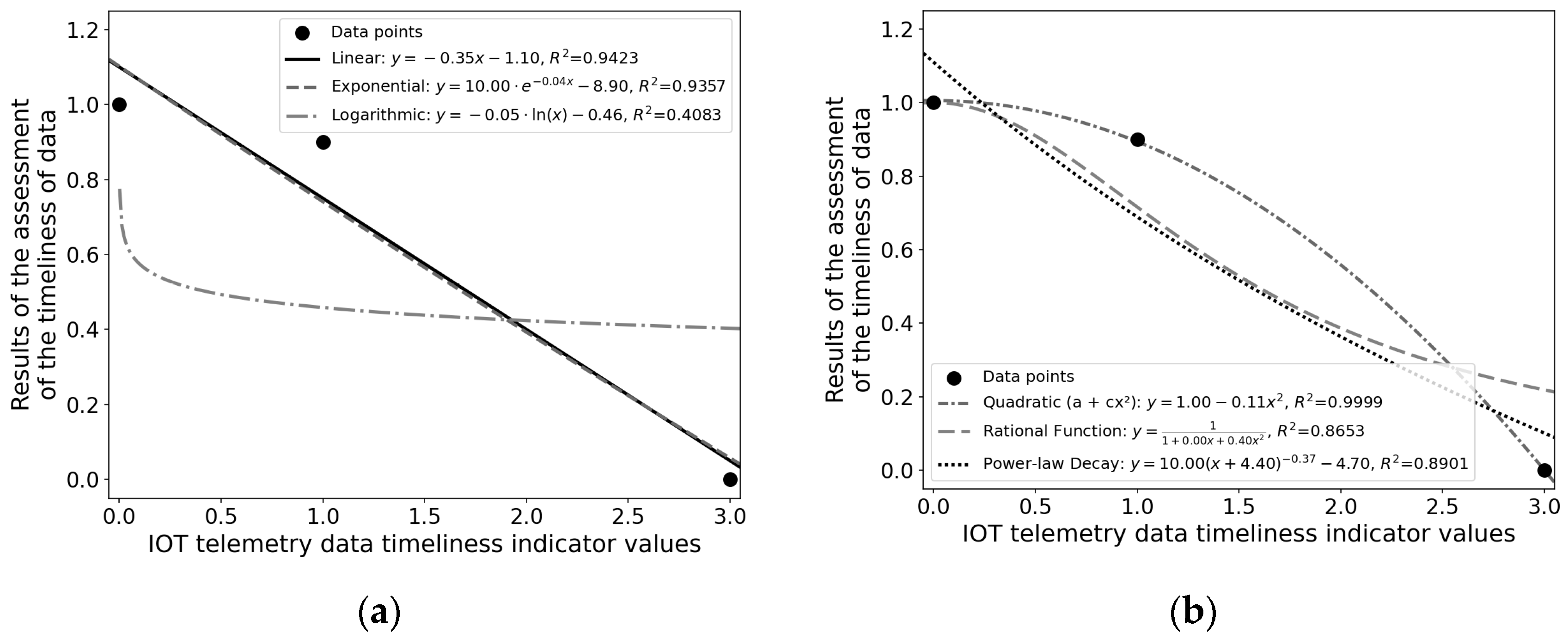
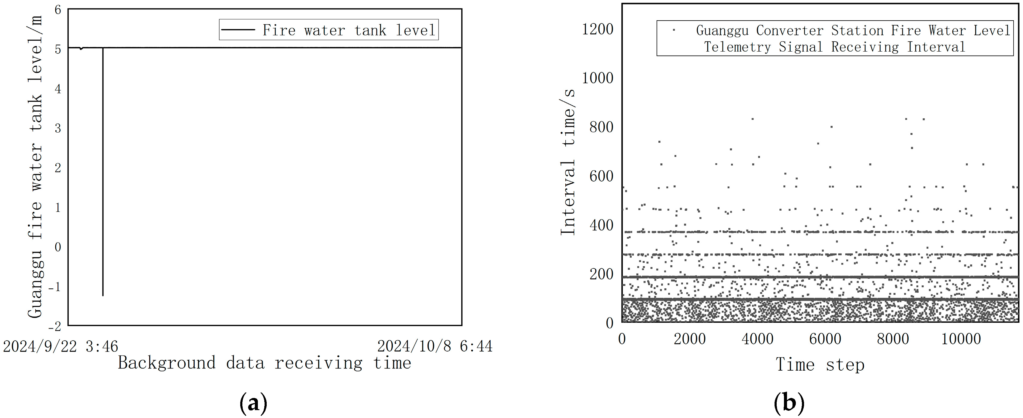
2.1.2. Data Timeliness Assessment

Telemetry time-series signals collected by sensors differ from telecontrol signals in that telemetry data are typically collected at regular intervals and involve large volumes of data. This requires buffering, processing, and transmission, which may result in significant delays between the data collection time and the time at which the monitoring center receives the data. Since telemetry signals will be used for further processing and analysis after quality evaluation, it is essential to provide a high-quality data foundation for subsequent applications. Therefore, ensuring uniformity in the data collection intervals is crucial. The timeliness of telemetry data is evaluated based on the time intervals between data uploads. The specific calculation follows this process, starting with the definition of time intervals:
Δ T n = T n T n 1  
where T n represents the time at which the n -th data are transmitted to the monitoring center backend, and Δ T n represents the transmission time interval between the n -th data and the preceding data.
The window size is set to N . The timeliness indicator of the time series data is related to the mean and standard deviation of the transmission time intervals of the previous N data points. The timeliness indicator I for the n -th data point is expressed as:
I n = Δ T n μ A σ A
where μ A is the mean of set A , σ A is the standard deviation of set A , and set A is [ Δ T n 1 , Δ T n 2 , , Δ T n N ] . A larger value of the parameter N necessitates accumulating more data to compute the timeliness indicator I , leading to longer computation times. Conversely, it enhances stability, resulting in smaller variations in parameters such as the mean and standard deviation. Assuming a constant rated sampling interval of the equipment, a larger N yields a computed mean that converges closer to this rated interval. However, if the rated sampling interval changes within the relevant time period, a larger N causes the mean parameter to respond more sluggishly to the change, diminishing adaptability. In contrast, a smaller N requires less accumulated data and shorter inference times. The trade-off is potentially greater volatility in the mean and standard deviation parameters within the time period. The advantage lies in its stronger adaptability: when the rated sampling interval is modified, the mean parameter converges more rapidly to the new rated value.
This study recorded the distribution of the timeliness indicator I for fire pool liquid level data in converter stations under different N values. The result is shown in Figure 4
At N = 10 , a significant number of data points exhibited I > 0.5 .
At N = 1000 , the distribution of I values was relatively uniform across the interval [1.5, 3.5].
At N = 10,000 , the number of data points with I values in the interval [2.5, 3.0] exceeded those in the interval [2.0, 2.5], contradicting the expectation that larger I values should exhibit sparser distributions.
Considering the balance among stability, adaptability, and computational resource consumption, N = 100 produced the most reasonable gradient in the I value distribution and was identified as the optimal choice.
Timeliness evaluation function: The metric I n , calculated by formula (6), represents the timeliness metric value at the n-th timestep. The magnitude of I n indicates the degree to which the data upload interval at that timestep deviates from the mean interval observed in the preceding time window. This deviation magnitude is determined by the mean and standard deviation of the intervals within that prior window, respectively. After obtaining the timeliness indicator I n , an evaluation function needs to be established. When I n = 0 , the timeliness evaluation y n = 1 , meaning that the data collection time intervals are completely uniformly distributed. During the actual operation of the converter station, it is desirable for the majority of data points to achieve high timeliness scores. As evidenced in Figure 4, data points with I n 1 constitute the predominant portion. Consequently, a timeliness score of y 1 (denoting “Excellent”) is assigned to data where I n 1 . This criterion ensures that the timeliness scores for most data points exceed 0.9. Finally, I n = 3 corresponds to the three-standard-deviation threshold in statistics. Given that the data transmission intervals in IoT systems are theoretically stable, any data exceeding this threshold are deemed a timeliness anomaly based on statistical principles, and assigned a timeliness score of y = 0 . Various regression models, such as linear regression, polynomial regression, exponential regression, and logarithmic regression, are considered. The regression results of each model are shown in Figure 5. Ultimately, the polynomial regression model yields the largest R value and the simplest expression. The regression equation is:
y = 1 0.11 I 2
After obtaining the validity score y and timeliness score δ for each time step data point in the time series, the composite quality of the time step data is obtained in the form of weighting. The data quality obtained at each time step will serve two purposes. First, it will be recorded for use in subsequent equipment health assessments, enabling early replacement and maintenance of equipment. Second, it will be used for subsequent data processing and application, such as time series prediction or other models, where it will serve as a reliability weight. The lower the data quality, the less useful the data will be due to the reliability weight.

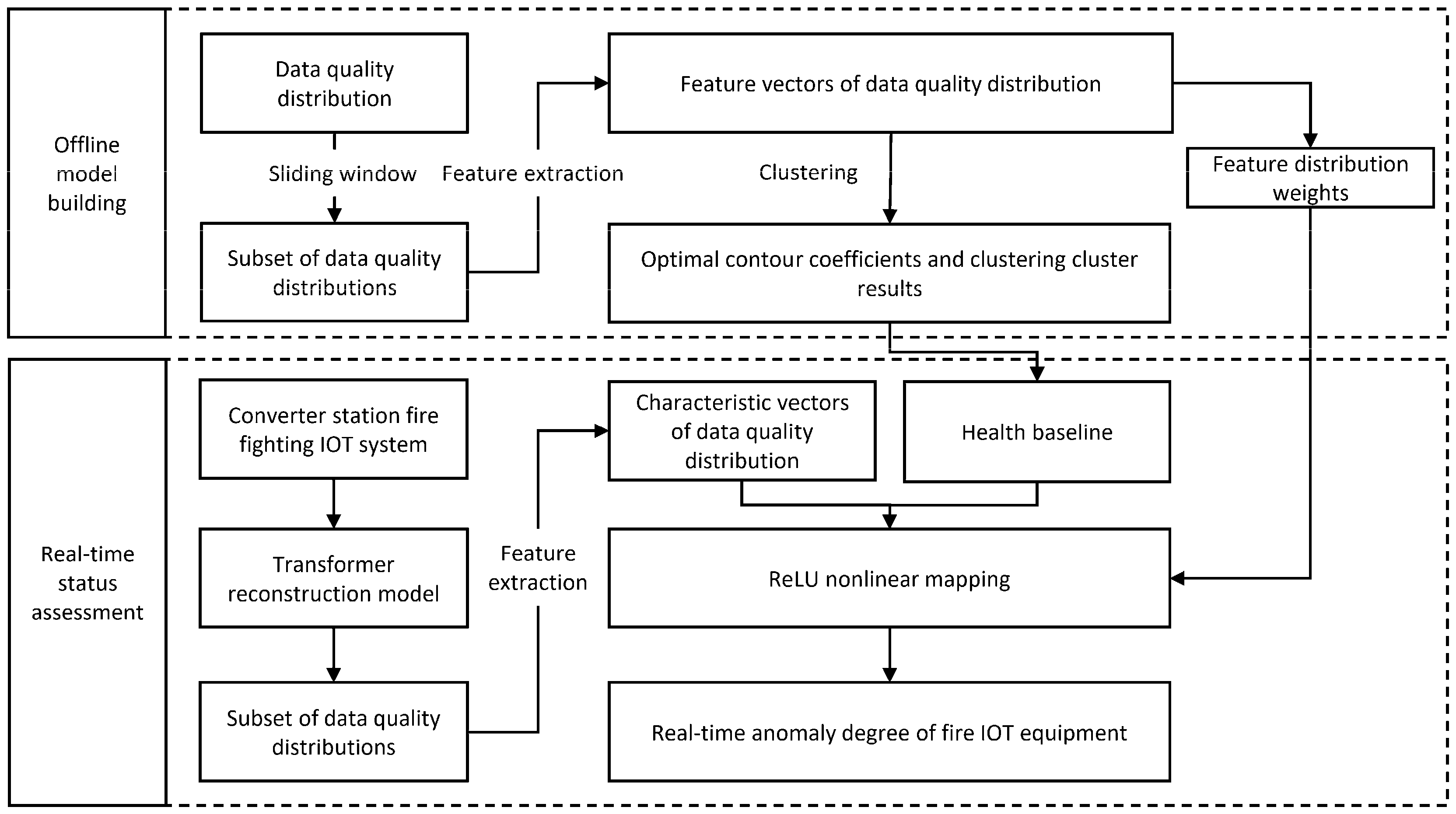
2.2. Device Health State Assessment Based on Integrated Data Quality

The overall framework of the evaluation is shown in Figure 6.

2.2.1. Feature Extraction Based on Sliding Time Window

Setting the length of the timing sliding window and sliding step to obtain the samples, the quality of the timing data in the window is converted into four-dimensional feature vectors, and the extraction rules are shown in Table 1.

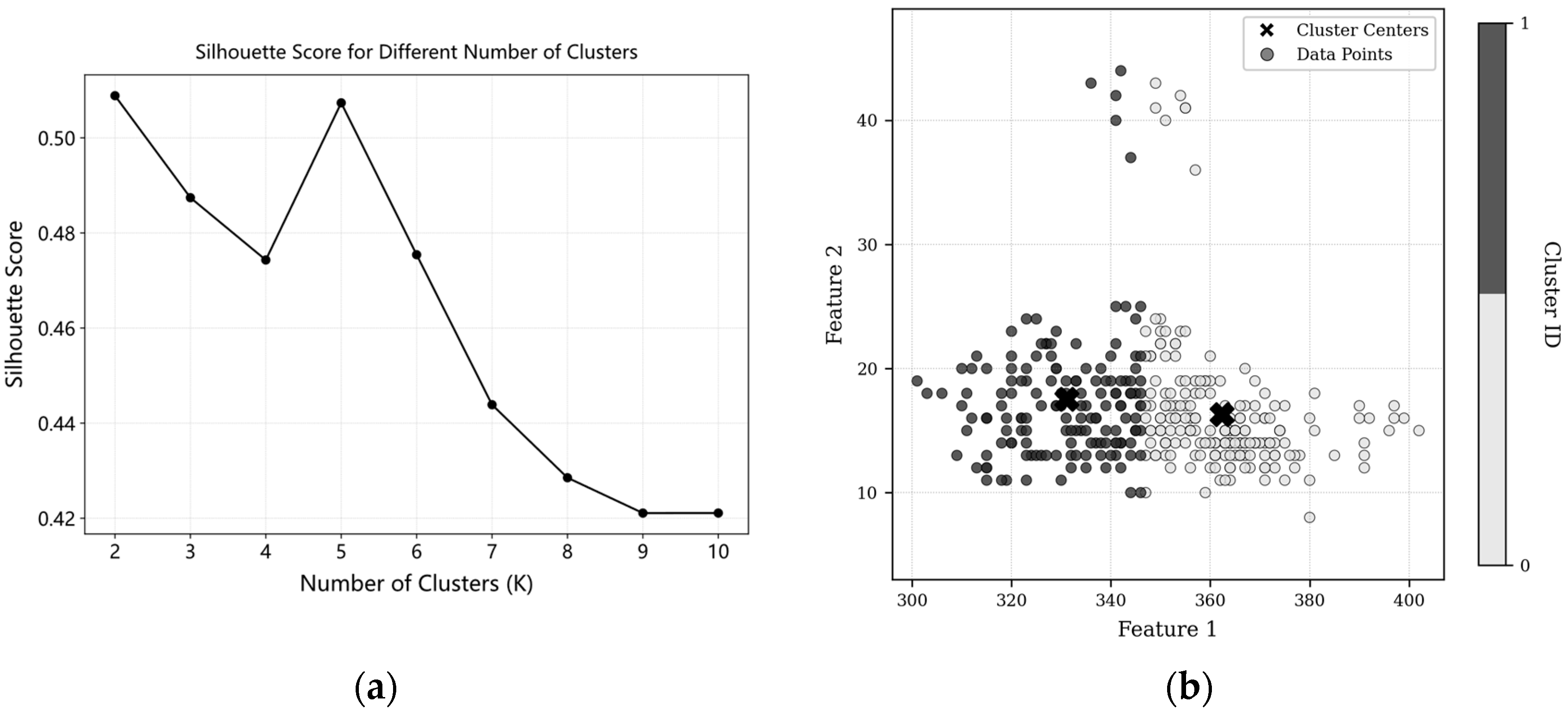
2.2.2. K-Means++ Clustering with Silhouette Coefficient

After processing with a sliding window, a large number of feature vectors representing healthy device states are obtained as samples. Once the sample set is acquired, the optimal number of clusters is determined automatically using the silhouette coefficient, and the K-means++ clustering algorithm is applied to identify the four-dimensional feature centers of each cluster.
The silhouette coefficient takes into account two aspects:
  • Cohesion: the average distance a ( i ) between a data point and other points in the same cluster;
  • Separation: the average distance b ( i ) between the data point and points in the nearest neighboring clusters.
The silhouette coefficient for each data point is calculated using the following formula:
s i = b i a i max a i , b i  
The silhouette coefficient ranges from −1 to 1. A value closer to 1 indicates better clustering performance, while a value closer to −1 suggests that a data point may have been misclassified. By computing the average silhouette coefficient of all data points, the overall performance of the clustering model can be comprehensively evaluated, and the optimal number of clusters k can be determined.
In the initialization phase of K-means++ clustering, the first cluster center is randomly selected from the dataset. Subsequently, the remaining cluster centers are chosen based on a probability P ( x ) , which is proportional to the squared distance from each data point to its nearest already-selected cluster center:
P ( x ) = D ( x ) x X D ( x )
where D ( x ) is the squared distance from data point x to its nearest existing cluster center. This strategy ensures a more reasonable distribution of initial cluster centers, thereby improving the clustering performance of the K-means++ algorithm.
In both K-means++ clustering and silhouette coefficient computation, Euclidean distance is used. This is a common method for calculating the straight-line distance between two points. For two points P ( x 1 , x 2 , , x n ) and Q ( y 1 , y 2 , , y n ) in an n-dimensional space, the Euclidean distance is defined as:
d P , Q = i = 1 n x i y i 2  
The value d P , Q represents the Euclidean distance between two points. During the normal operation of fire protection IoT devices, various working conditions may arise, and the representative feature vectors under different conditions can differ significantly. Consequently, clustering with k = 1 may fail to effectively distinguish between these working conditions. By introducing the silhouette coefficient, it becomes possible to identify representative feature vectors corresponding to different operating conditions in a high-dimensional feature space—i.e., the feature vectors represented by the cluster centers. This not only enhances the interpretability of the model, but also improves its robustness.
Ultimately, the cluster centers obtained through K-means++ are regarded as the most representative healthy sample feature vectors, serving as the health baselines for equipment evaluation.

2.2.3. ReLU Nonlinear Mapping Model

After obtaining the health baselines, the ReLU nonlinear mapping model is used to evaluate the distance between real-time samples and the health baselines. The distance is affected by the difference between each feature of the feature vector and the corresponding feature in the health baseline, as well as by the feature weights. The feature weights consist of two components: importance weights and distribution-based weights.
In terms of importance weights, different data quality levels inherently have different levels of importance. Therefore, the importance weights A W i are set as follows: A W 1 = 0.1 , A W 2 = 0.2 , A W 3 = 0.3 , and A W 4 = 0.4 .
The distribution-based weights are determined using the entropy weight method. X i j represents the value of the j -th indicator for the i -th sample. During the application of the entropy weight method, the first step is to normalize the data:
Y i j = X i j min X i max X i min X i
According to the definition of information entropy in information theory, the entropy E of each feature j in a dataset is calculated using the following formula:
E j = k i = 1 n p i j log p i j
p i j = Y i j i = 1 n Y i j
where k is a constant typically set as k = 1 / ln ( n ) , where n is the total number of feature vector samples obtained under the normal operating conditions used in clustering. After computing the information entropy for each indicator as E 1 , E 2 , …, E m , the weight R V i of each indicator is calculated based on its entropy using the following formula:
R V i = 1 E i i = 1 m ( 1 E i )
where m is the total number of features. When the information is more concentrated, the entropy becomes smaller and the corresponding weight becomes larger. The combined weight ω i is defined as:
ω i = θ R V i i = 1 m R V i + ( 1 θ ) A W i i = 1 m A W i
After obtaining the feature weights, the deviation degree of a feature vector within a specific time window from the representative feature vector under normal operating conditions can be calculated. The number of clusters and the cluster set C = { C 1 , C 2 , , C n } are obtained through clustering. Let Z denote all samples in the i -th cluster C i , i.e., Z = { z 1 , z 2 , , z m } , where m is the number of samples in the i -th cluster. A single feature vector sample z a = [ x a 1 , x a 2 , x a 3 , x a 4 ] consists of four features, and the cluster center is denoted as z 0 , whose feature vector is obtained through the clustering method and expressed as z 0 = [ x 01 , x 02 , x 03 , x 04 ] .
Assume that the feature vector data used for clustering are all obtained from the normal operation of healthy equipment, thus, it is assumed that each feature vector falls within the range representing health. The confidence interval for the k -th feature of this cluster, which is determined as normal, can be defined as [ x 0 k d k min , x 0 k + d k max ] , where d k min and d k max represent the minimum and maximum distance from the feature value of the k -th feature to the cluster center, respectively, and can be expressed as:
d k m i n = α [ x 0 k min i [ 1 , m ] ( x i k ) ]
d k m a x = α [ max i [ 1 , m ] ( x i k ) x 0 k ]
where, α is the confidence coefficient used to expand the range, generally greater than 1. In the process of calculating the anomaly score, we consider the anomaly score only when it exceeds the confidence range. Therefore, the commonly used ReLU function in deep learning is introduced. When the input is greater than 0, the output of the ReLU function is equal to the input itself; when the input is less than or equal to 0, the output of the ReLU function is 0.
For a new feature vector sample point n , its feature vector is [ x 1 , x 2 , x 3 , x 4 ] , and the anomaly score δ n is calculated as follows:
δ n = i = 1 k ω i ReLU [ f ( x i ) ] N
f ( x i ) = x 0 k d k m i n x i ,   When   x i < x 0 k x i x 0 k d k m a x ,   When   x i > x 0 k
where ω i is the combined weight of the feature i and x 0 k is the value of the k -th feature corresponding to the cluster center of the new sample. For a cluster, each feature has a unique d k min and d k max . N is the scale parameter, where N = x 01 + x 02 + x 03 + x 04 , representing the total number of telemetry data points collected during a certain period for that cluster center. The equipment that collects more data over a period of time is more likely to capture more abnormal data, which results in the last two feature values of the feature vector being larger than those of equipment with a smaller data collection volume. Therefore, this method is used as a normalization approach.
Ultimately, the anomaly score δ n is used to represent the health status of the converter station’s fire IoT equipment. When the equipment is healthy, δ n equals 0, and when the equipment is abnormal, the anomaly score increases, causing the value of δ n to rise as well.

3. Results

In this study, experiments were conducted on real telemetry data collected at the converter station to measure the effectiveness assessment results of the transformer reconfiguration model and the health status assessment results of the fire IOT equipment, and to compare the assessment performance of different models.

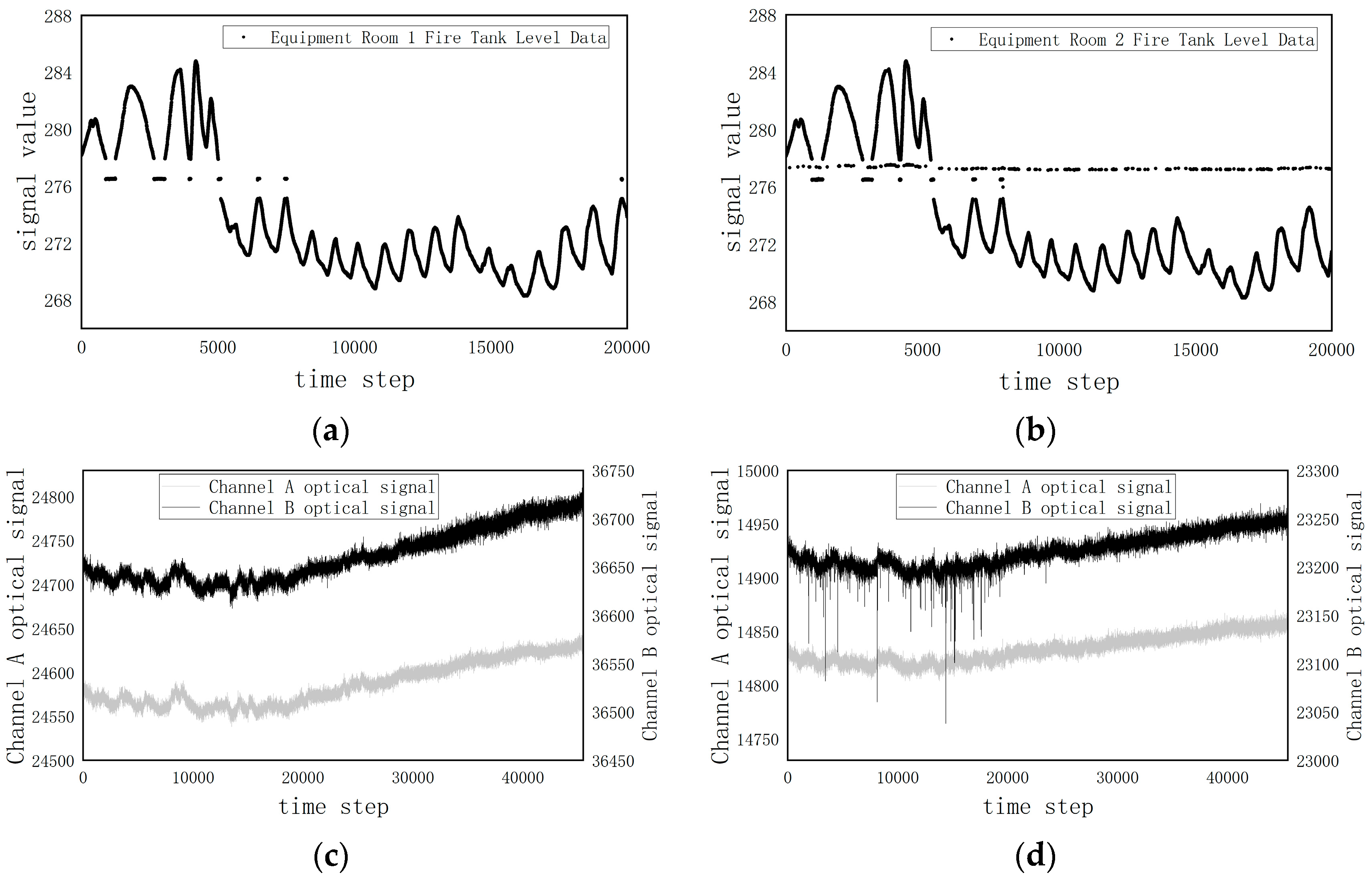
3.1. Results of the Data Validity Assessment

To validate the model’s effectiveness and generalizability, two sets of real-world time-series data containing outliers were used to validate the model. The first dataset was sourced from water tank level data of equipment at the Yibin Substation. Although the data from the two devices exhibited trend consistency, the water level of the second device showed continuous jumps. The raw data are shown in Figure 7a,b. The second dataset was derived from the time-series dual-channel optical signals of smoke detectors collected indoors. By comparing with other smoke detectors in the same period, it was found that the optical signal of channel B of a certain detector exhibited anomalies. The raw data are shown in Figure 7c,d.
The parameters of the transformer reconstruction model are shown in the Table 2 below.
Figure 7. Time-series data source ((a) Yibin Converter Station tank water level—Equipment 1 tank water level; (b) Yibin Converter Station tank water level—Equipment 2 tank water level; (c) Time-series data from normal smoke detectors during the same period; (d) Time-series data from anormal smoke detectors during the same period).
Fire 08 00251 g007
For converter station water level data, the data collected from equipment room 1 are treated as normal data, and the data collected from equipment room 2 are treated as abnormal data. First, the normal data are used for training, and the reconstruction error threshold is obtained from the reconstruction error of the normal data. The abnormal data are then fed into the trained model to obtain the reconstruction error distribution. The reconstruction error threshold is used to identify abnormal points and obtain the validity score of subsequent data. The reconstruction results and reconstruction error distribution are shown in Figure 8 and Figure 9:
For smoke detection time series data, an unsupervised learning method was used, with the time series data themselves, including outliers, serving as the model training data to obtain the reconstruction error and the threshold for identifying outliers. The results are shown in Figure 10 and Figure 11, which also prove that the training data can contain a small number of outliers.
Finally, taking the water tank level data in the converter station equipment room as an example, the relevant parameters of the data validity assessment function are obtained. Based on the anomaly threshold ε = 0.00365165 and setting δ l = 0.8 , the calculated value of β = 111.03613657 , and the score δ ( i ) is obtained as follows:
δ ( i ) = 2 2 1 + e 111.03613657 e i
The final data validity evaluation results are shown in Figure 12.
Finally, this study compares the transformer reconstruction model with LSTM (long short-term memory network), GRU (gated recurrent unit), and TCN (temporal convolutional network) for two types of time series. Additionally, three threshold selection methods were compared: the 95th percentile, the three-standard-deviation, and the POT (peak over threshold) extreme value theory-based method. The comparison was conducted under identical conditions, including the same loss function, optimizer, number of iterations, batch size, and learning rate, to evaluate the anomaly detection performance of each model and threshold selection method.
This study labeled all abnormal points in the two time series, with the time series length and number of abnormal points shown in Table 3. Model performance was evaluated using accuracy, precision, recall, and F1 score. The results are shown in Table 4.
As shown in Table 4, for the two fire-related time series, the transformer reconstruction model combined with the POT extreme value theory achieved the best results in anomaly detection. Due to the low proportion of anomalies, the three-standard-deviation method and the 95th percentile method classified a large amount of normal data as anomalies, resulting in high recall rates, but low precision for the model.
Finally, we also tested the inference speed comparison after model training to measure the computational efficiency of different models. The single inference latency measurement was based on a single standard input sample (shaped as [1,2,20]), and 10,000 independent inferences were performed on an NVIDIA RTX 4060 device to obtain the average value. The results are shown in Table 5.
The inference latency results demonstrate that all models maintain rapid processing speeds with two hidden layers, rendering them suitable for deployment on computationally constrained platforms. Nevertheless, the transformer architecture exhibited the longest inference latency due to its inherent complexity.

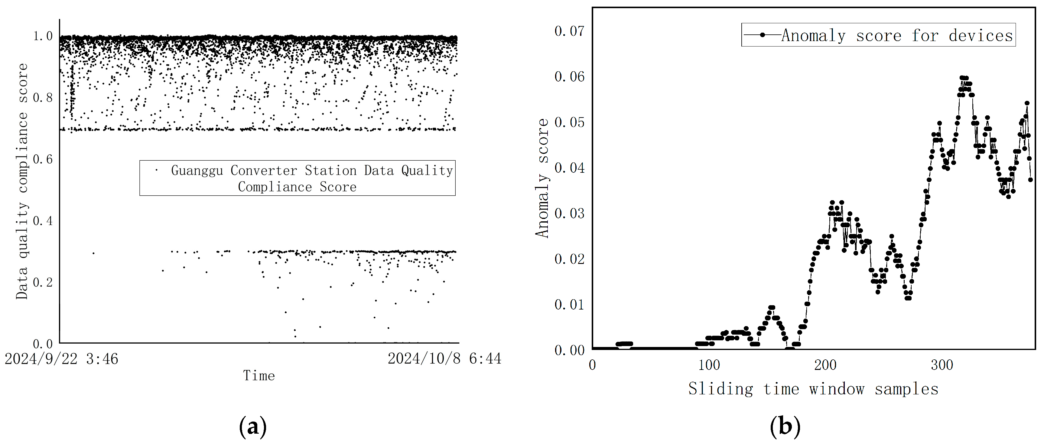
3.2. Results of the Device Health Status

Taking the remote telemetry data of the fire pool water level at the Guanggu Converter Station as an example, the water level values and data collection intervals are shown in Figure 13a,b:
Among them, the validity assessment adopts the transformer reconstruction model proposed above with the automatic threshold acquisition method of POT extreme value theory, and the timeliness assessment is carried out in accordance with the evaluation function above, taking into account that the telemetry data pay more attention to the accuracy of the data rather than the timeliness, so the weights of the validity and timeliness are [0.7, 0.3], and the weighted results of the comprehensive assessment of the data quality obtained in the weighted data quality are shown in Figure 14.
From Figure 13b and Figure 14, it can be seen that timeliness affects the degree of integrated data quality to the greatest extent, and the time sequence data-receiving time interval in 80–100 s accounts for the highest percentage of time sequence data, which can be regarded as the collection time interval set by the IOT sensors in the range of 80–100 s, whereas the time interval between neighboring water level telemetry data received by the backend of the actual monitoring center can be up to 20 min. In addition to this, the single-point jump anomaly in the original timing data can be seen in Figure 14, which also converts to a lower data quality score.
After excluding the time window where the single-point anomaly is located, the remaining time window is identified as fault-free for equipment health baseline extraction, the length of the sliding time window is set to 12 h, the step size is set to 1 h, and the optimal contour coefficient is 2. Since the values of features 3 and 4 in the health sample obtained in Figure 14 are both zero, the clustering of the first two features is demonstrated, and the clustering results are shown in Figure 15.
According to the health state assessment model to obtain the combination of weights, health baseline, and health upper and lower limits, the results are shown in Table 6. The weight of information entropy and the weight of importance are both 50%.
To test the reasonableness of the anomaly assessment, jump anomalies were injected into the raw data, where the first 25% of the data were kept as raw data, and the time step was in the interval from 25% to 50%, with 1% jump anomalies, and the anomalies consistent with its own intrinsic anomalies, i.e., −1.25 m; the next 25% were injected with 5% jump anomalies, and the last 25% were injected with 10% jump anomalies.
The final comprehensive quality distribution of telemetry equipment data is shown in Figure 16a, the results of equipment anomaly evaluation are shown in Figure 16b, and the eigenvalues of some samples are shown in Table 7.
Also, in comparison with the use of Euclidean distance and cosine distance as a baseline measure of distance to health at the sample points, each distance measure was normalized to show only the trend of the data, and the results are shown in Figure 17.
As shown in Figure 17, using the ReLU function, the feature vectors generated by the firefighting equipment in the non-failure state have a score of 0, which is different from the Euclidean distance and cosine distance methods. In addition, it can be seen that the proposed method of obtaining the degree of abnormality combined with objective weights can better reflect the degree of deviation of “urgent” and “critical” in the feature vector of each sample point, and can reflect the importance of different features, and has a high degree of stability. It can better measure the current state of the equipment corresponding to the sample points.

4. Conclusions

This paper proposes a data-driven framework for equipment health assessment in fire IoT systems at converter stations, combining data quality evaluation with interpretable state analysis. The main contributions are summarized as follows:
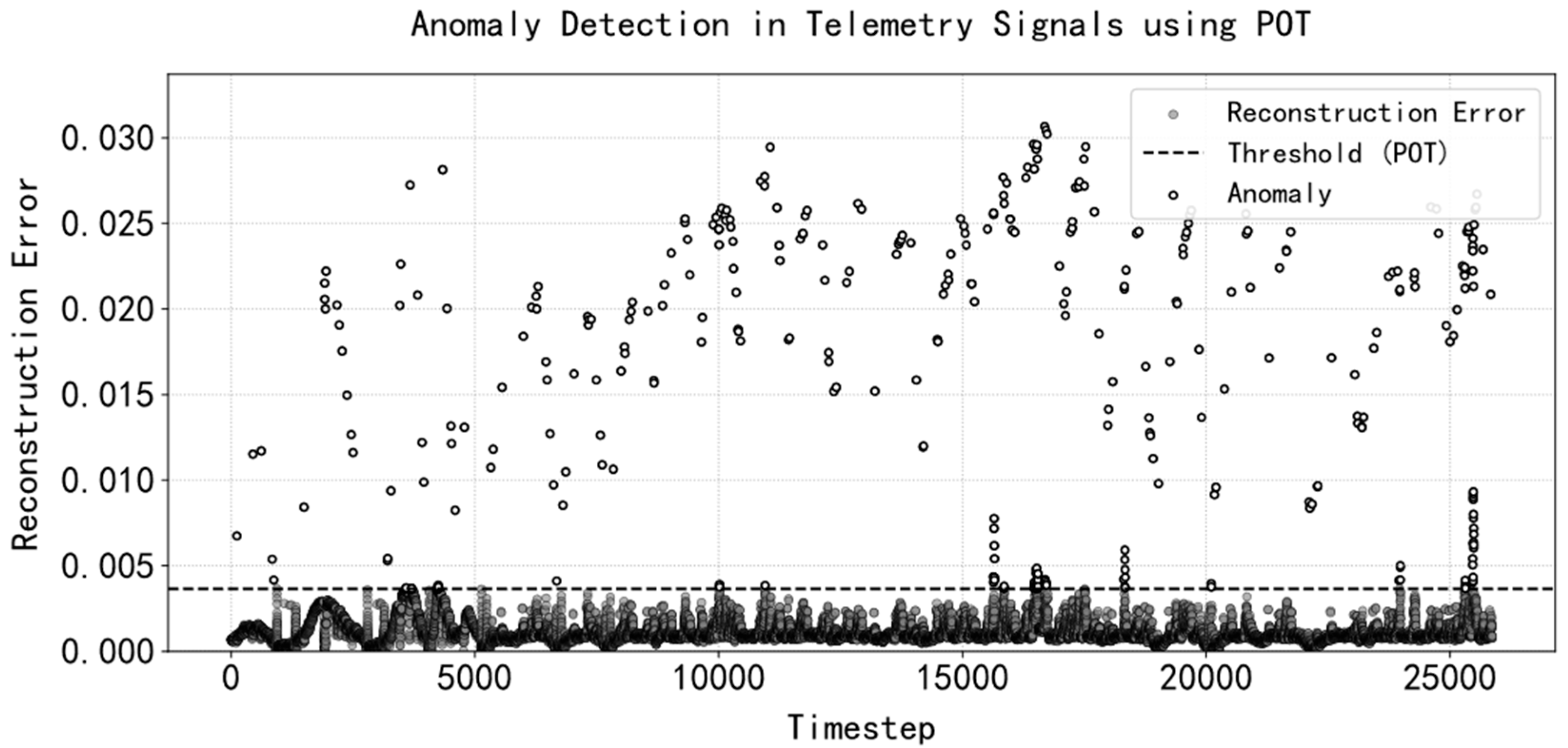
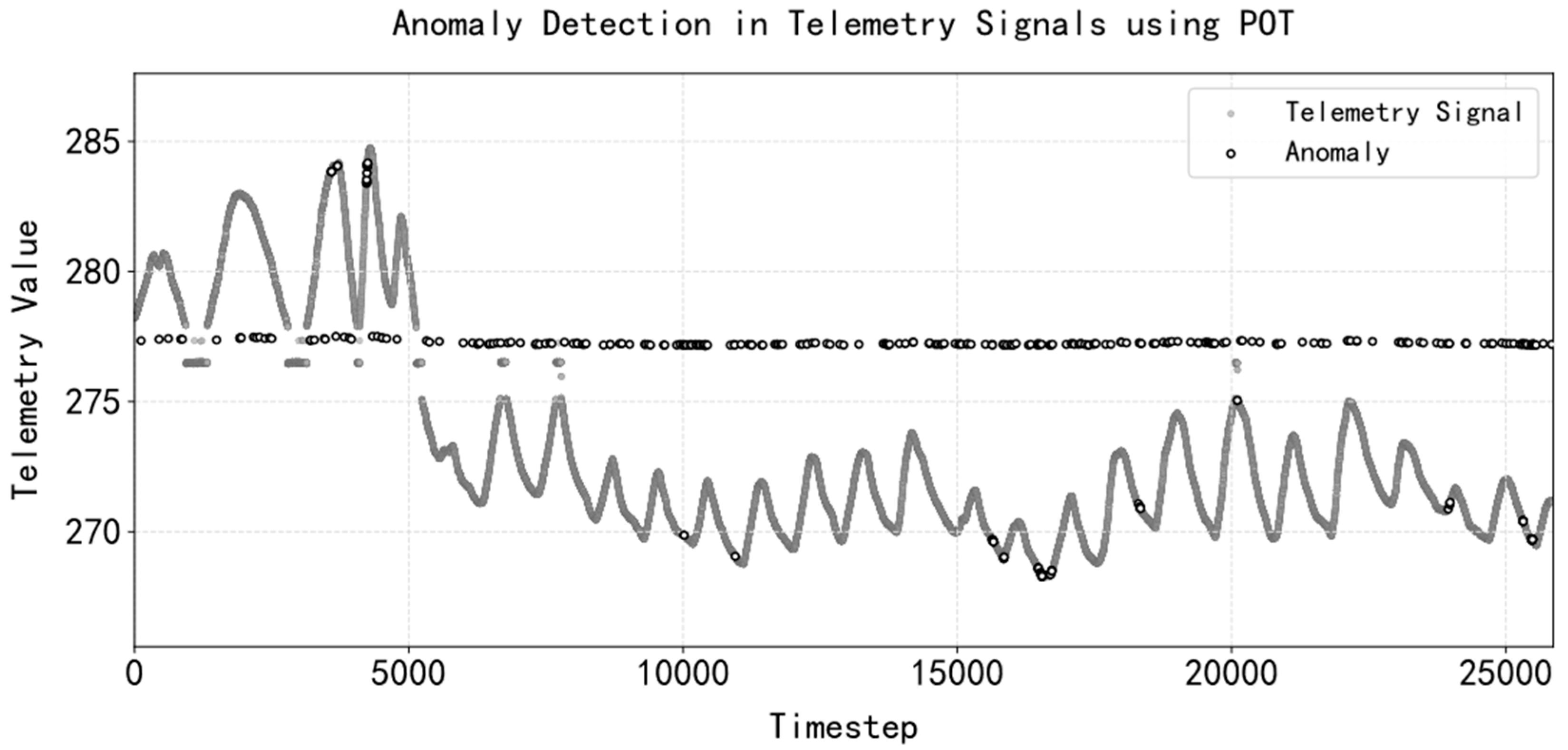
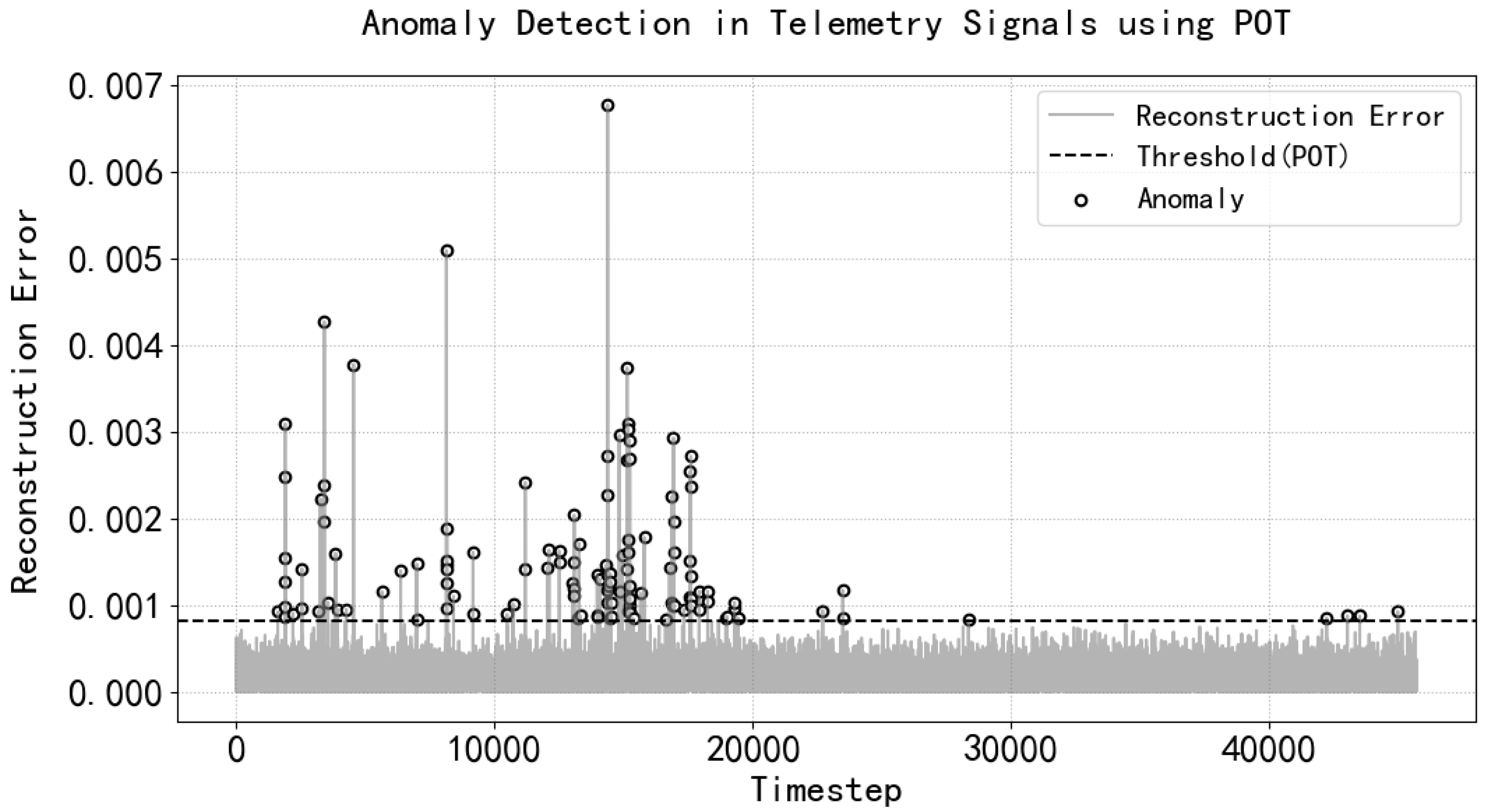
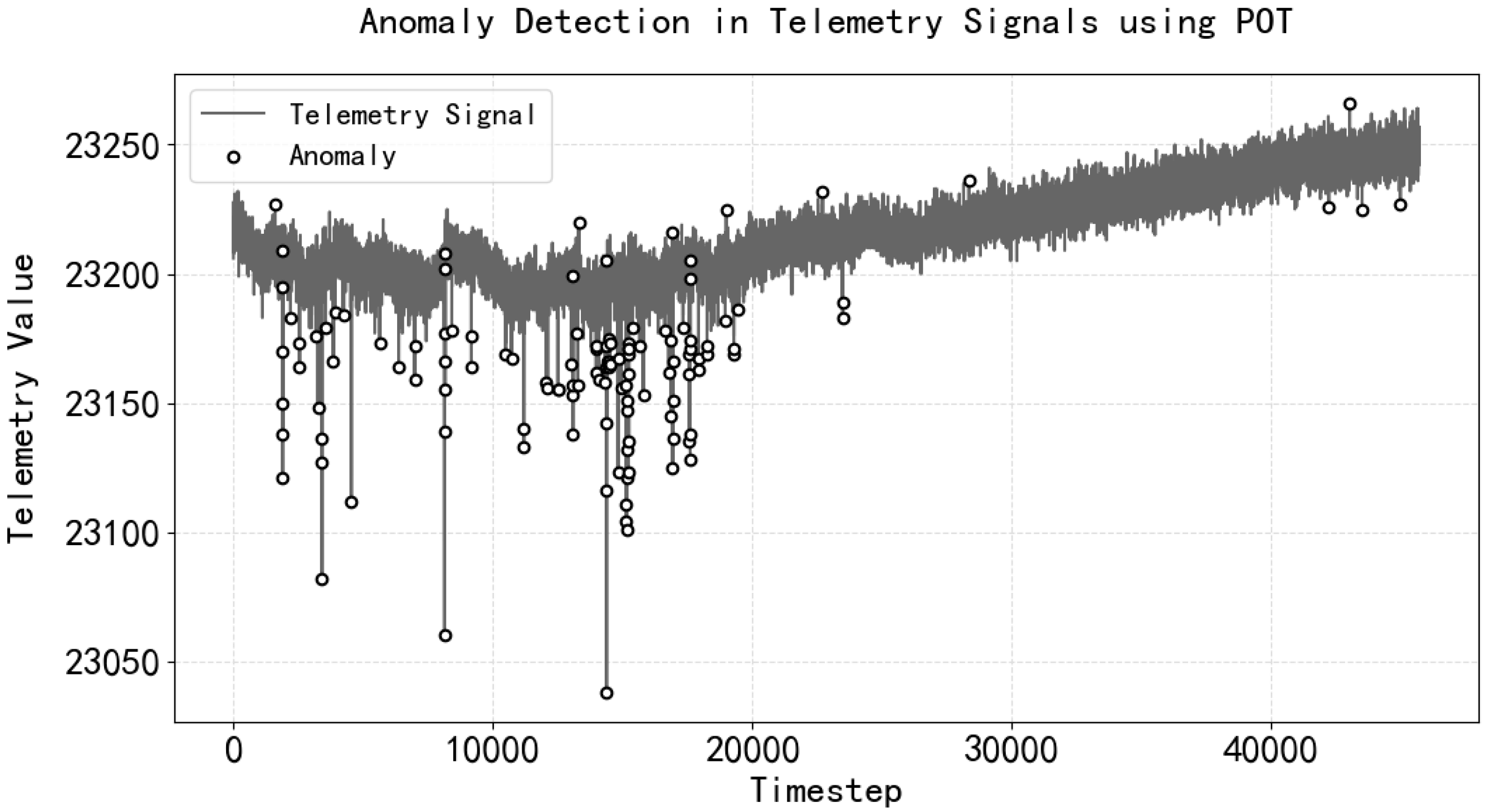
  • Validity Assessment with Temporal Reconstruction: A transformer-based sequence reconstruction model integrated with POT (peaks over threshold) anomaly detection was developed to evaluate data credibility. This method effectively identifies tiny jump anomalies through temporal pattern learning and achieves an F1 score of 0.83 on real telemetry data collected at the converter station. Compared with LSTM, TCN, and GRU, the F1 of the transformer model constructed in this case is higher, and other models will have a large amount of normal time-step data that are judged as abnormal by the reconstruction error thresholds, which makes the model’s recall higher and its precision lower;
  • Timeliness Quantification Framework: We choose the optimal number of windows and design simple and practical timeliness evaluation functions;
  • Interpretable Health Scoring System: Based on the comprehensive quality of the data, a feature extraction method is designed to cluster the extracted features and combine them with an objective evaluation method to measure the degree of deviation between the real-time operating state and the health state of the equipment, so as to derive the degree of abnormality of the equipment.
The key innovations of this research lie in:
  • Deep Learning-Enhanced Data Quality Assessment: In the traditional method of measuring the comprehensive quality of data, only the threshold value is used to judge the validity of the data, while the introduction of the deep learning method into the comprehensive quality assessment of data can well discriminate minor anomalies and uncover potential anomalies before the state of health does not deteriorate rapidly;
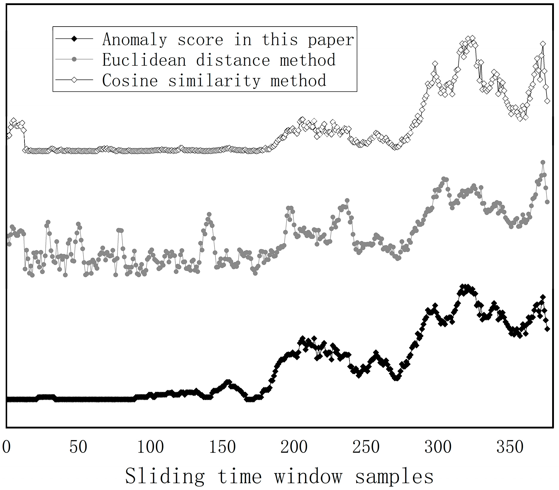
  • Highly Interpretable Fire Equipment Health Assessment: The health state assessment starts from the comprehensive quality of each data point, and the final evaluation results are highly interpretable compared with those of gray models, such as machine learning. And the model can also be used to detect whether the equipment is abnormal, as well as to assess the degree of abnormality. We use the ReLU function so that the device has an anomaly score of 0 in the absence of anomalies, which is superior to the commonly used methods for assessing distance;

5. Future Work

While this framework provides a robust foundation for fire IoT equipment health assessment, there are still several tasks that we will continue to work on in the future:
  • Advanced Utilization of Comprehensive Data Quality Metrics: While this study applied data quality metrics to equipment health assessment, future work will explore novel applications of these metrics as independent time-series inputs. This includes integrating quality scores into potential models, such as predictive analysis and temporal correlation analysis, to improve the stability of the converter station fire protection system;
  • δ n -BasedHealth State Taxonomy and Maintenance Framework: In this study, device anomaly scores were proposed to measure the severity of device faults. Currently, a device anomaly score of 0 indicates that the device is healthy, while a non-zero score indicates an anomaly, with higher values indicating greater severity. In future research, more on-site device information will be collected and combined with device anomaly scores to obtain device health status grades, which will be used to construct replacement and maintenance management strategies for fire protection devices.
  • Compare the Influence of Different Clustering Algorithms on the Assessment of Health Status: In this study, we used K-means clustering to obtain health status. Currently, we lack quantitative indicators to measure the impact of different clustering algorithms on health status results. In the future, we will accumulate more real anomaly data and develop a quantitative indicator to describe the accuracy of health status identification, similar to describing and verifying forest fire risks, in order to measure the impact of different clustering algorithms on equipment health status assessment and select the most appropriate clustering method.
  • Implement actual deployment and address corresponding challenges: In this study, we aim for the health status evaluation model to detect faults originating from the fire-protection IoT device itself, such as transmission delays or faulty data caused by performance degradation. However, in real-world scenarios, external factors such as strong electromagnetic interference or network failures may affect the stability of telemetry signals. This can result in the model failing to detect actual device faults and, in some cases, mistakenly identifying multiple devices as abnormal. Therefore, mitigating the influence of such external interferences—including electromagnetic and network-related disruptions—on the model’s diagnostic capability is an important aspect of our future work. In the future, we plan to deploy the model in real fire-protection IoT environments, testing it on various devices and types of time-series data, while specifically evaluating its response and robustness to network failures, sensor faults, and background interferences.

Author Contributions

Conceptualization, J.Z. and Y.H.; methodology, Y.H. and T.S.; validation, Y.C., Z.Y., and T.Y.; formal analysis, Y.H.; investigation, Z.Y.; resources, J.Z.; data curation, T.Y.; writing—original draft preparation, Y.H.; writing—review and editing, Z.Y.; visualization, Y.C.; supervision, T.Y.; project administration, Y.H.; funding acquisition, J.Z. All authors have read and agreed to the published version of the manuscript.

Funding

This research was funded by Science and Technology Project for State Grid Anhui Electric Power Co., Ltd., grant number B3120523000D.

Institutional Review Board Statement

Not applicable.

Informed Consent Statement

Not applicable.

Data Availability Statement

The original contributions presented in this study are included in the article. Further inquiries can be directed to the corresponding author(s).

Acknowledgments

During the preparation of this study, the authors utilized the fire protection equipment status data provided by the Advanced Technology Research Institute of the University of Science and Technology of China to verify the reliability of the analytical method. For this, the authors express their gratitude.

Conflicts of Interest

Authors Yubiao Huang, Tao Sun, Yifeng Cheng, Jiaqing Zhang were employed by the company State Grid Anhui Electric Power Research Institute. The remaining authors declare that the research was conducted in the absence of any commercial or financial relationships that could be construed as a potential conflict of interest.

References

  1. Bianco, A.M.; Martinez, E.J.; Ben, M.G.; Yohai, V.J. Robust Procedures for Regression Models with ARIMA Errors. In COMPSTAT.; Prat, A., Ed.; Physica-Verlag HD: Heidelberg, Germany, 1996; pp. 27–38. [Google Scholar]
  2. Hernandez-Garcia, M.R.; Masri, S.F. Application of Statistical Monitoring Using Latent-Variable Techniques for Detection of Faults in Sensor Networks. J. Intell. Mater. Syst. Struct. 2014, 25, 121–136. [Google Scholar] [CrossRef]
  3. Samparthi, V.K.; Verma, H.K. Outlier Detection of Data in Wireless Sensor Networks Using Kernel Density Estimation. Int. J. Comput. Appl. 2010, 5, 28–32. [Google Scholar] [CrossRef]
  4. Gu, Y.; Deng, H. Fault Analysis of Pipeline System Sensor Based on K-Nearest Neighbor Algorithm. Chin. J. Sens. Actuators 2017, 30, 1076–1082. [Google Scholar]
  5. Arias, L.A.S.; Oosterlee, C.W.; Cirillo, P. AIDA: Analytic Isolation and Distance-Based Anomaly Detection Algorithm. Pattern Recognit. 2023, 141, 109607. [Google Scholar] [CrossRef]
  6. Wu, D. Research on deep learning-based anomaly data recognition method for structural health monitoring system. Intell. City 2020, 6, 10–13. [Google Scholar]
  7. Hooshmand, M.K.; Hosahalli, D. Network Anomaly Detection Using Deep Learning Techniques. CAAI Trans. Intell. Technol. 2022, 7, 228–243. [Google Scholar] [CrossRef]
  8. Audibert, J.; Michiardi, P.; Guyard, F.; Marti, S.; Zuluaga, M.A. USAD: UnSupervised Anomaly Detection on Multivariate Time Series. In Proceedings of the 26th ACM SIGKDD International Conference on Knowledge Discovery & Data Mining, San Diego, CA, USA, 23–27 August 2020; ACM: New York, NY, USA, 2020; pp. 3395–3404. [Google Scholar]
  9. Gao, H.; Chen, Z.; Zhou, F.; Li, D.; Yang, K.; Shi, X. Abnormal Identification of Oil Monitoring Data Based on Classification-Driven SAE. In 2022 Global Reliability and Prognostics and Health Management (PHM-Yantai); IEEE: New York, NY, USA, 2022; pp. 1–6. [Google Scholar]
  10. Darban, Z.Z.; Webb, G.I.; Pan, S.; Aggarwal, C.C.; Salehi, M. CARLA: Self-Supervised Contrastive Representation Learning for Time Series Anomaly Detection. Pattern Recognit. 2025, 157, 110874. [Google Scholar] [CrossRef]
  11. Zhang, Z.; Cheng, D.; Liu, N.; Yang, H. Research and Implementation of Conformity Testing Method for Military Information System Information Exchange Standards. J. CAEIT 2019, 14, 1242–1248. [Google Scholar]
  12. Yin, R.; Yao, Z. Research on Data Quality Assessment Framework for Multidisciplinary Standards. Stand. Sci. 2020, 1, 92–95. [Google Scholar]
  13. Zhu, H.; Gao, A.; Wang, S. Research on Conformance Testing of Data Standard. Stand. Sci. 2019, 7, 53–57. [Google Scholar]
  14. Yang, J.; Guo, J. Design of Observation Data Quality Assessment Model of CINRAD. Stand. Sci. 2021, 12, 123–127, 144. [Google Scholar]
  15. Zheng, P. Evaluation index system of compliance test for information business collaboration standards. J. Fuzhou Univ. (Nat. Sci. Ed.) 2021, 49, 747–752. [Google Scholar]
  16. Nabhan, A.; Ghazaly, N.; Samy, A.; Mousa, M.O. Bearing Fault Detection Techniques-a Review. Turk. J. Eng. Sci. Technol. 2015, 3, 1–18. [Google Scholar]
  17. Helbing, G.; Ritter, M. Deep Learning for Fault Detection in Wind Turbines. Renew. Sustain. Energy Rev. 2018, 98, 189–198. [Google Scholar] [CrossRef]
  18. Udu, A.G.; Lecchini-Visintini, A.; Dong, H. Feature Selection for Aero-Engine Fault Detection. In Database and Expert Systems Applications; Springer: Cham, Switzerland, 2023; pp. 522–527. [Google Scholar]
  19. Tayarani-Bathaie, S.S.; Vanini, Z.S.; Khorasani, K. Dynamic Neural Network-Based Fault Diagnosis of Gas Turbine Engines. Neurocomputing 2014, 125, 153–165. [Google Scholar] [CrossRef]
  20. Cao, X.; Duan, Y.; Zhao, J.; Yang, X.; Zhao, F.; Fan, H. Summary of research on health status assessment of fully mechanized mining equipment. J. Mine Autom. 2023, 49, 23–35, 97. [Google Scholar]
  21. Hao, X.; Liu, X.; Li, X.; Zhao, X. Research on Online Safety Precaution Technology of a High-Medium Pressure Gas Regulator. J. Therm. Sci. 2017, 26, 229–234. [Google Scholar] [CrossRef]
  22. Gao, F.; Li, H.; Wu, F. Health Status Monitoring and Fault Diagnosis Based on Spectrum Analysis for Centrifugal Pump. Process Autom. Instrum. 2019, 40, 24–28. [Google Scholar]
  23. Hu, Y.; Ping, B.; Zeng, D.; Niu, Y.; Gao, Y.; Zhang, D. Research on Fault Diagnosis of Coal Mill System Based on the Simulated Typical Fault Samples. Measurement 2020, 161, 107864. [Google Scholar] [CrossRef]
  24. Aker, E.; Othman, M.L.; Veerasamy, V.; Aris, I.b.; Wahab, N.I.A.; Hizam, H. Fault Detection and Classification of Shunt Compensated Transmission Line Using Discrete Wavelet Transform and Naive Bayes Classifier. Energies 2020, 13, 243. [Google Scholar] [CrossRef]
  25. Choudhary, A.; Mian, T.; Fatima, S. Convolutional Neural Network Based Bearing Fault Diagnosis of Rotating Machine Using Thermal Images. Measurement 2021, 176, 109196. [Google Scholar] [CrossRef]
  26. Zhao, J.H. Research on Anomaly Detection of Mine CO Sensor Based on Variational Autoencoder. Master’s Thesis, Xi’an University of Science and Technology, Xi’an, China, 2024. [Google Scholar]
  27. Sousa Tomé, E.; Ribeiro, R.P.; Dutra, I.; Rodrigues, A. An Online Anomaly Detection Approach for Fault Detection on Fire Alarm Systems. Sensors 2023, 23, 4902. [Google Scholar] [CrossRef] [PubMed]
Figure 1. Overall flowchart of device health condition assessment.
Fire 08 00251 g001
Figure 2. Timing data validity scoring flowchart.
Fire 08 00251 g002
Figure 3. Transformer reconfiguration model structure diagram.
Fire 08 00251 g003
Figure 4. Distribution histogram of timeliness indicator vs. window size ((a) Results of the distribution of timeliness indicator values at N = 10; (b) Results of the distribution of timeliness indicator values at N = 100; (c) Results of the distribution of timeliness indicator values at N = 1000; (d) Results of the distribution of timeliness indicator values at N = 10,000).
Fire 08 00251 g004
Figure 5. Regression results of various models. ((a) Regression results for linear, exponential, and logarithmic functions; (b) Regression results for quadratic, rational function, and power-law decay functions).
Fire 08 00251 g005
Figure 6. Overall framework for real-time condition assessment of fire protection IoT equipment.
Fire 08 00251 g006
Figure 8. Relative reconstruction error anomaly threshold for water tank level data.
Fire 08 00251 g008
Figure 9. Identification of abnormal points in remote sensing time sequence signals of water tank liquid levels based on abnormal thresholds.
Fire 08 00251 g009
Figure 10. Relative reconstruction error anomaly threshold for smoke detector data.
Fire 08 00251 g010
Figure 11. Identification of abnormal points in remote sensing time sequence signals of smoke detector data based on abnormal thresholds.
Fire 08 00251 g011
Figure 12. Effectiveness evaluation results based on the transformer model and the POT threshold method.
Fire 08 00251 g012
Figure 13. Original telemetry data of Guanggu fire water tank level and signal reception time interval ((a) Guanggu fire water tank level telemetry data; (b) Signal reception time interval of Guanggu Converter Station fire water tank level).
Fire 08 00251 g013
Figure 14. Comprehensive scoring of the quality of telemetry data of the fire water tank level at Guanggu Converter Station.
Fire 08 00251 g014
Figure 15. Clustering results of feature vectors from sliding window samples of Guanggu fire water tank level ((a) Silhouette coefficients for different K values; (b) KMeans++ clustering results).
Fire 08 00251 g015
Figure 16. Comprehensive scoring of data quality and anomaly score for abnormal liquid level data of Guanggu fire water tank ((a) Comprehensive scoring of the quality; (b) Anomaly score evaluation results).
Fire 08 00251 g016
Figure 17. Comparison of three distance measurement methods.
Fire 08 00251 g017
Table 1. Four-dimensional extraction rule for feature vectors.
Data Quality Category
(Score Range)
Variable in Feature VectorMeaning of Variable
General
(0.80–1.00)
x1Number of data points within the sliding window assessed as general (normal) quality
Minor
(0.60–0.80)
x2Number of data points within the sliding window assessed as minor anomaly
Urgent
(0.40–0.60)
x3Number of data points within the sliding window assessed as urgent anomaly
Critical
(0.00–0.40)
x4Number of data points within the sliding window assessed as critical anomaly
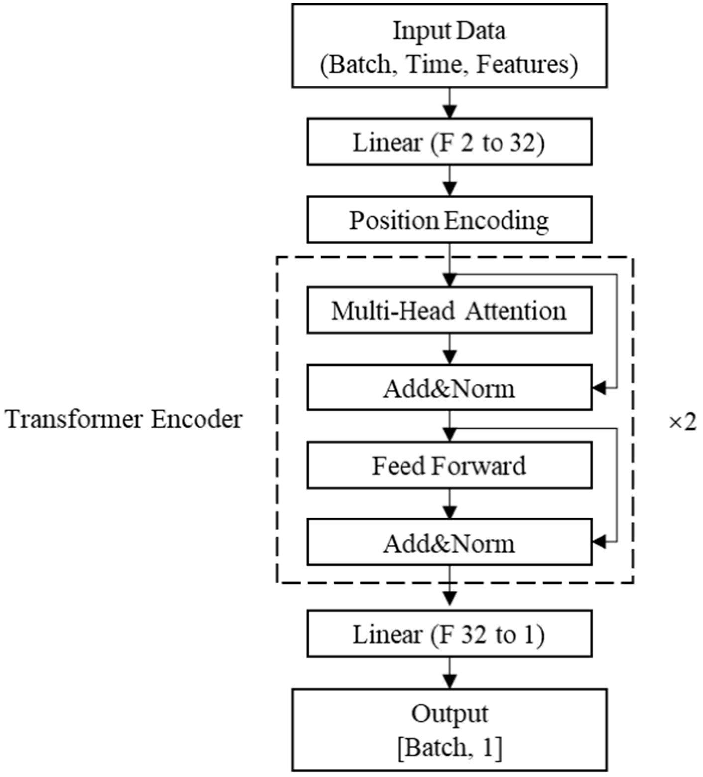
Table 2. Transformer neural network-related parameters.
ParameterValue
Loss FunctionMSE (mean-squared error)
OptimizerAdam
Number of Epochs100
Batch Size256
Learning Rate0.001
Number of Attention Heads8
Number of Encoder Layers2
Input Sequence Length20
Feature Dimension2
Table 3. Time-series data information containing outliers.
NameTime Series LengthNumber of AnomaliesPercentage of Anomalies/%
Yibin Converter Station Equipment 2 tank water level25,8652721.0516
Indoor smoke detector channel B optical signal45,694950.2079
Table 4. Performance comparison of models.
Time Series Data NameThreshold Selection MethodMetricModel
LSTMGRUTCNTransformer
Converter Station Tank Water LevelPOTAccuracy0.89650.93900.97280.9957
Precision0.09230.14660.27850.7238
Recall1.00000.99630.99630.9632
F1 score0.16890.25550.43530.8265
μ + 3 σ Accuracy0.83530.85320.89590.9539
Precision0.06000.06680.09150.1845
Recall1.00001.00000.99630.9890
F1 score0.11320.12530.16760.3110
95th
percentile
Accuracy0.69870.68980.71830.9314
Precision0.03370.03280.03590.1326
Recall1.00001.00000.99630.9963
F1 score0.06520.06350.06920.2340
Smoke
Detector Channel B Optical Signal
POTAccuracy0.99680.99820.99640.9988
Precision0.34730.55470.26970.6694
Recall0.61050.74740.43160.8737
F1 score0.44270.63680.33200.7580
μ + 3 σ Accuracy0.99160.99190.99000.9941
Precision0.16080.18740.11540.2569
Recall0.72630.87370.56840.9789
F1 score0.26340.30860.19180.4070
95th
percentile
Accuracy0.95130.95170.95080.9521
Precision0.03370.03810.02890.0416
Recall0.81050.91580.69471.0000
F1 score0.06470.07310.05550.0798
The bolded part in the table represents the combination of the optimal deep learning model and threshold selection method for each performance parameter.
Table 5. Model single-sample inference time.
Model
LSTMGRUTCNTransformer
Average Latency Ms0.46 ± 0.070.44 ± 0.080.57 ± 0.100.97 ± 0.15
Table 6. Health baselines and feature weights from KMeans++ clustering.
ClusterParameterx1x2x3x4
Cluster 1Health Lower Bound345.4610.2200
Health Baseline362.3718.8100
Health Upper Bound397.1648.7200
Combined Weight0.06570.13050.37190.4319
Cluster 2Health Lower Bound301.2710.1300
Health Baseline331.3319.7300
Health Upper Bound347.4740.9300
Combined Weight0.06570.13050.37190.4319
Table 7. Results of anomaly scores for samples injected with anomalies (partial).
Samplesx1x2x3x4Anomaly Score
134437000
235736000
374286190360.0469
375293190330.0418
376301180300.0372
Ellipses (...) were used to indicate omitted items within the table.
Disclaimer/Publisher’s Note: The statements, opinions and data contained in all publications are solely those of the individual author(s) and contributor(s) and not of MDPI and/or the editor(s). MDPI and/or the editor(s) disclaim responsibility for any injury to people or property resulting from any ideas, methods, instructions or products referred to in the content.

