Article

A Near-Real-Time Operational Live Fuel Moisture Content (LFMC) Product to Support Decision-Making at the National Level

by
Akli Benali
1,*,
Giuseppe Baldassarre
1,
Carlos Loureiro
2,
Florian Briquemont
1,3,
Paulo M. Fernandes
4,
Carlos Rossa
4,5 and
Rui Figueira
6
1
Forest Research Centre, Associate Laboratory TERRA, School of Agriculture, University of Lisbon, 1349-017 Lisboa, Portugal
2
Instituto da Conservação da Natureza e das Florestas, IP. Parque Florestal, 5000-567 Vila Real, Portugal
3
Bruxelles Environnement Tree Management, Service Avenue du Port 86C/3000, 1000 Brussels, Belgium
4
Centre for Research and Technology of Agro-Environmental and Biological Sciences, CITAB, Inov4Agro, University of Trás-os-Montes and Alto Douro, UTAD, Quinta de Prados, 5000-801 Vila Real, Portugal
5
School of Technology and Management (ESTG), Polytechnic of Leiria, Apartado 4163, 2411-901 Leiria, Portugal
6
CIBIO, Centro de Investigação em Biodiversidade e Recursos Genéticos, InBIO Laboratório Associado, Instituto Superior de Agronomia, Universidade de Lisboa, Tapada da Ajuda, 1349-017 Lisboa, Portugal
*
Author to whom correspondence should be addressed.
Fire 2025, 8(5), 178; https://doi.org/10.3390/fire8050178
Submission received: 7 March 2025 / Revised: 24 April 2025 / Accepted: 28 April 2025 / Published: 30 April 2025

Abstract

:
Live fuel moisture content (LFMC) significantly influences fire activity and behavior over different spatial and temporal scales. The ability to estimate LFMC is important to improve our capability to predict when and where large wildfires may occur. Currently, there is a gap in providing reliable near-real-time LFMC estimates which can contribute to better operational decision-making. The objective of this work was to develop near-real-time LFMC estimates for operational purposes in Portugal. We modelled LFMC using Random Forests for Portugal using a large set of potential predictor variables. We validated the model and analyzed the relationships between estimated LFMC and both fire size and behavior. The model predicted LFMC with an R2 of 0.78 and an RMSE of 12.82%, and combined six variables: drought code, day-of-year and satellite vegetation indices. The model predicted well the temporal LFMC variability across most of the sampling sites. A clear relationship between LFMC and fire size was observed: 98% of the wildfires larger than 500 ha occurred with LFMC lower than 100%. Further analysis showed that 90% of these wildfires occurred for dead and live fuel moisture content lower than 10% and 100%, respectively. Fast-spreading wildfires were coincident with lower LFMC conditions: 92% of fires with rate of spread larger than 1000 m/h occurred with LFMC lower than 100%. The availability of spatial and temporal LFMC information for Portugal will be relevant for better fire management decision-making and will allow a better understanding of the drivers of large wildfires.

1. Introduction

Fire regimes are shaped by four main processes: the existence of spatially continuous biomass, the vegetation’s availability to burn (i.e., dryness), meteorological conditions conducive to fire spread, and ignitions [1]. When all these processes, or “switches”, are no longer limiting factors, the conditions for the occurrence of large wildfires are met. Fuels play an important role in determining when part of these “switches” are activated. The amount of fine biomass (i.e., fine fuel load), its arrangement and its moisture content directly activate the first two “switches”, also influencing fire behavior [2]. Indirectly, fuel dryness also influences the probability of an ignition being successful [3], contributing to the activation of the fourth “switch”.
Fuel moisture content (FMC) is the quantity of water per dry mass of fuel. Fuels have dead and live components that have different associated moisture contents governed by different mechanisms [4]. The dead fuel moisture content (DFMC) responds closely to weather variations and is mediated by local conditions affecting solar radiation, exhibiting pronounced daily and intra-daily fluctuations [5]. Live fuel moisture content (LFMC) is typically one order of magnitude larger than DFMC [4] and depends on environmental conditions (e.g., soil moisture, vapor pressure deficit) and ecophysiological responses (e.g., soil water uptake, plant water storage), with smooth daily and seasonal variations. In terms of fuel types, LFMC in shrublands responds to environmental changes slower than in grasslands due to their distinct ecophysiological responses [6].
LFMC (and FMC in general) influences fire activity and behavior because drier vegetation requires less energy and time for water to partially vaporize, thus influencing fire ignition and spread [3,7,8]. The ability to estimate LFMC throughout the year and over large areas is important to improve our capability to predict when and where large and intense wildfires may occur [9]. There is strong evidence that LFMC influences fire activity at large temporal and spatial scales, as burned area tends to increase when fuels are more homogeneously dry across the landscape [6,10,11,12]. This evidence has been incorporated in operational fire danger metrics (e.g., [13]).
The relation between LFMC and fire behavior has been controversial [9]. Several authors have suggested that the effect of LFMC on fire behavior and its relevance in an operational context is marginal [14,15]. However, others have shown a strong relation between LFMC and the forward rate of spread (ROS) based on laboratory [8] and field experiments [16]. According to Pimont et al. [9], the relation between LFMC and ROS is strong and the discrepancies between prior studies could be due to the modelling approach used, the range of LFMC data, the use of small datasets and the impact of random measurement error. In addition, LFMC has an annual evolution trend correlated with monthly DFMC (e.g., Mediterranean shrubs) and, as a result, the effect of LFMC is very difficult to detect from field data [17]. Jolly [2] found that the sensitivity of modelled fire behavior to LFMC was highly dependent on the proportion of live and dead fuel loads. Thus, monitoring LFMC and incorporating it in operational models can be useful for better decision-making [9,18]. Currently, the operational models using LFMC as an input, respectively to predict crown and surface fire behavior, are the Canadian Forest Fire Behavior Prediction System [19] and US fire behavior prediction tools based on the model of Rothermel (e.g., FARSITE [20]). However, the Rothermel [21] model was developed from laboratory experiments in dead fuels and mathematically extended to account for the effect of live fuels [22].
LFMC can be estimated from fieldwork by collecting live vegetation samples and oven-drying at 105 °C to estimate the dry and fresh weight [23] or using alternative methods [24]. Although field sampling provides valuable data, the process is laborious and costly [6]. Additionally, it is difficult to obtain representative samples over a wide temporal and spatial range. Often, spatial interpolation is required to tackle the latter limitation, which in turn has its own limitations. These issues can hinder the application of LFMC sampling for operational purposes.
Alternatively, methods based on satellite, soil, vegetation and meteorological data have been employed to tackle the limitations of field sampling. Most of these methods commonly use either statistical or radiative transfer modelling [6]. Statistical models fit satellite and/or meteorological data to sampled LFMC and can be extrapolated to similar areas [25,26,27]. This approach has been widely used to estimate LFMC [28,29,30,31]. Radiative transfer modelling relies on physical equations that relate satellite-derived reflectance with plant water content [32,33]. Its extrapolation to larger areas is possible but more complex than statistical modelling. A noteworthy approach is the development of a global-scale LFMC product using radiative transfer modelling [34]. These studies have contributed to a better estimation of LFMC across a wide range of spatial and temporal scales, improving predictive capabilities across different ecosystems.
The availability of near-real-time LFMC estimates during the fire season is very limited, hindering our capability of quantifying the availability of vegetation to burn, and consequently predicting where and when large wildfires can occur. Estimating LFMC based on previously calibrated models can fill an existing gap in operational decision-making. However, LFMC modelling has limitations associated with reproducing lower extreme values [28], lack of validation for global-scale model parameterization [34], limited generalization of models [35], reliance on single-season data and small sample sizes [29,36], and the coarse resolution of input data [30,31]. In addition, near-real-time LFMC estimates require models that are properly calibrated with data that is available with low latency.
The objective of this work is to develop a near-real-time LFMC dataset for operational purposes in a fire-prone country like Portugal. This will tackle existing research and operational gaps, contributing to better situational awareness and decision-making. To achieve this goal, we first model LFMC using Random Forests based on sampled LFMC for Portugal and a large set of potential predictor variables. We then validate the model at both global and site level and assess the relationships between LFMC and fire size and behavior to evaluate the dataset’s consistency and potential usefulness.

2. Materials and Methods

2.1. LFMC Sampling and Data Processing

In 2019, the Agency for Integrated Management of Rural Fires (AGIF) and the Institute for Forest and Nature Conservation (ICNF) started collecting LFMC samples across Portugal’s mainland territory, employing a varying schedule that predominantly spans between April and October. The selection of sampling sites was made by operatives (Figure 1) and was based on (i) operational factors (e.g., availability of trained technicians, distance to post-processing facilities); (ii) accessibility; (iii) areas with less than 20% tree cover, more than 50% shrub cover and with southern quadrant exposure. Sampling was done between 14:00 and 15:00, randomly selecting different plants in the plot. Sampling sites number 10 and 6 correspond to the new locations of sites 9 and 12, respectively, due to accessibility reasons. Sampling focused on three primary fuel types: pine tree needles, shrubs and herbs. Our analysis focused on shrub LFMC due to its importance in determining fire behavior in Portugal, but also due to the comparatively lower number of samples collected for the remaining fuels.
The fuel samples were obtained by clipping terminal live foliage and twigs (<3 mm diameter) with pruning shears. The material was collected from various shrubs at diverse heights and places in the crown, comprising a mixture of new and older growth, and was transported in tightly-sealed glass containers of known weight. The samples were processed in the laboratory within 1–2 h after collection. Each container was weighed in an electronic scale to the nearest 0.1 g and then opened and put in a forced-convection oven where it stayed for 48 h at 100 °C to obtain the sample dry weight.
A total of 1023 shrub LFMC samples were available, spanning from June 2019 to October 2022. The diversity of samples at each site was contingent upon the species encountered there, as indicated in Table 1. AGIF and ICNF identified anomalous values during sample collection that were screened. These discrepancies were identified by comparison with previous and posterior LFMC values and nearby sites, often caused by improper handling, mistakes during collection (i.e., samples containing flowers, fruits, or thicker woody material) or post-processing errors, causing anomalously high or low LFMC values. Following this rigorous screening, a total of 992 LFMC samples from 16 sampling sites were retained for subsequent analysis.
LFMC samples from different species collected on the same dates in the same site were aggregated into a composite sample to determine a mean shrub LFMC value. Only dates with comprehensive sampling across all species were included for locations hosting data from multiple species. It is important to mention that no information was available regarding the relative coverage of each individual species nor the height of the shrub vegetation.

2.2. LFMC Modelling

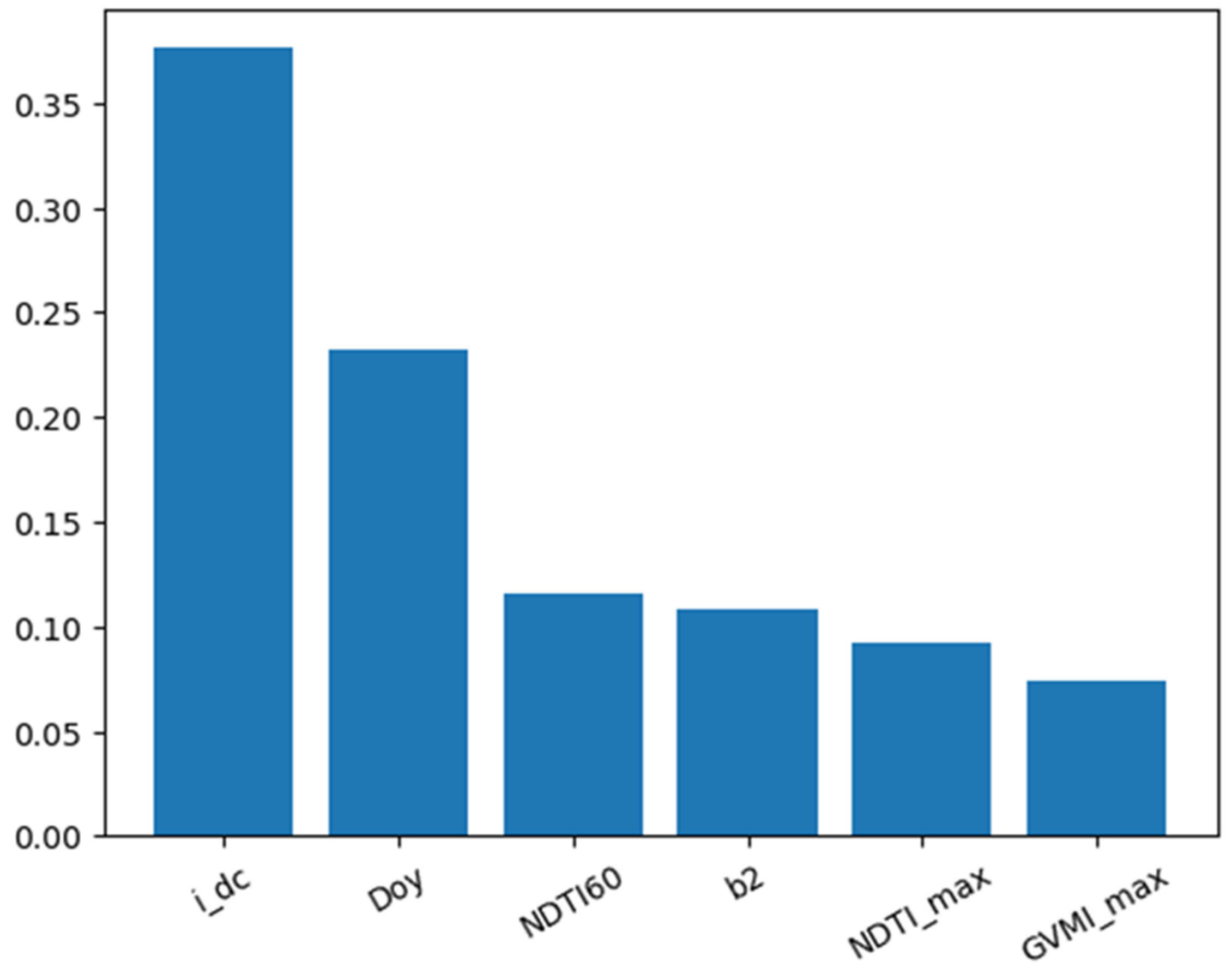
2.2.1. Predictor Variables

To comprehensively characterize potential environmental drivers influencing LFMC, we integrated data from different types: (i) satellite reflectances and spectral vegetation indices; (ii) Land Surface Temperature; (iii) vegetation maps; (iv) topography; (v) fire–weather indices; and (vi) auxiliary variables. Considering that the objective was to develop LFMC maps for mainland Portugal for operational purposes, we restricted the selection of possible sources to those that could provide data covering the entire country, had frequent coverage (when applicable) with moderate to high resolution, covered the period of LFMC sampling and were available in near-real time with low latency.
The satellite data used in this study were sourced from Google Earth Engine (GEE), a cloud-based platform for geospatial analysis [37]. The Moderate Resolution Imaging Spectroradiometer (MODIS) MCD43A4 version 6.1 dataset [38] provides a 500 m daily surface reflectance product and has been used previously for LFMC modelling [28,35]. SI are capable of mitigating directional anisotropic and soil background effects while accentuating distinctive attributes of the vegetation canopy [18]. A range of vegetation spectral indices (SI) were computed using daily surface reflectances (Table 2).
The MODIS Land Surface Temperature/Emissivity 8-Day (MOD11A2 [39]) was used due to its relevance in assessing water availability for plant evapotranspiration and consequent impacts on canopy temperature [18]. MOD11A2 provides an eight-day moving window average of land surface temperature (LST) estimates, derived from daily estimates, with a 1000 m resolution.
The impact of vegetation features on LFMC was reviewed following methodologies employed in previous studies [33,36]. The MOD44B.006 dataset [40] provides yearly Vegetation Continuous Fields (VCF) at a spatial resolution of 250 m providing estimates of percent vegetation, percent non-tree cover, and percent non-vegetated. Among these, “percent non-tree cover” was specifically considered as the shrub component at the subpixel level. Additionally, data from the Copernicus Global Land Service (CGLS), specifically the 2019 land cover dataset [41], were used. This dataset, available at a spatial resolution of 100 m, provides percentages of various land cover types including bare, crops, grass, shrub, tree, and urban.
Given the influence of topography on local climate, solar irradiance, and subsequently LFMC [17], the Shuttle Radar Topography Mission (SRTM) digital elevation data at 30 m resolution was used to characterize topographic features such as elevation, aspect, and slope [42]. Additionally, the ALOS Landform dataset [43] was used, providing landform classes at a resolution of 90 m.
The Canadian Fire Weather Index (FWI) provides fire danger estimates [44]. The system includes six sub-indices: the Fine Fuel Moisture Code (FFMC), which assesses the ignition potential of fine fuels; the Duff Moisture Code (DMC), which evaluates moisture content of decomposing organic material; the Initial Spread Index (ISI), which represents the rate of fire spread; the Build-Up Index (BUI), which gauges the amount of available fuel; and the Drought Code (DC), which reflects deeper drying in organic layers. FWI and its sub-indices are calculated based on relative humidity, temperature, wind speed and rainfall data. In this study, we used the dataset produced by the Portuguese Institute for Sea and Atmosphere [45] that provides FWI estimates based on daily meteorological observations and forecasts at noon (UTC), with a high spatial resolution of 1 km that results from interpolating data from 93 automatic weather stations across Portugal.
Additionally, we included as variables the day of year (DOY) and day length, as auxiliary variables to capture seasonal trends in LFMC dynamics [30,35]. DOY was normalized to the range [0, 1] and then transformed to the range [−π, π], ensuring consistent representation throughout the year. This transformation, as employed by Zhu et al. [35], involved computing the sine (DOY_SIN) and cosine (DOY_COS) values, preserving information on the nature of the annual cycle. Both DOY_SIN and DOY_COS values ranged from −1 to 1, where DOY_SIN captured variations from the wettest to the driest seasons, and DOY_COS reflected seasonal variations from winter (coldest) to summer (hottest).
For the majority of variables, we generated normalized values using a temporal rescaling method based on the maximum and minimum values within each extracted predictor’s time series [25]. This max–min scaling approach mitigated the effects of spatial and interannual variations in vegetation cover, facilitating the correlation of LFMC changes with meteorological drivers and reducing errors in LFMC estimates. Moreover, average values over 30, 60, and 80 days preceding the sampling date were calculated for most of the extracted predictors, provided in Table 3 along with their main characteristics. A total of 147 potential predictor variables were used.
For each LFMC sampling site, the extraction of the predictor variables was conducted by aligning with the spatial resolutions appropriate for the datasets in use. This involved adjusting the pixel sizes to ensure accurate and consistent sampling across various locations, using standardized techniques to average pixel values where necessary. This method ensures that all data extracted are suitable for subsequent analysis, regardless of the original resolution of the data source.

2.2.2. Modeling Using Random Forests

We used Random Forests (RF) modelling to estimate LFMC across mainland Portugal. RF is a non-parametric, machine learning technique that ensembles multiple decision trees to build a robust model to predict outcomes. This method, pioneered by Breiman [46], effectively handles large datasets with numerous variables without requiring prior knowledge of their interrelationships. Its resilience against outliers ensures reliable predictions [47].
When calibrating the RF algorithm, it is necessary to specify certain hyperparameters. These include the total number of trees (n_estimators), maximum number of variables (or features) randomly selected at each split (max_features), and the maximum number of levels in each decision tree (max_depth). A systematic exploration of the set of potential inputs was conducted through a grid-search scheme combined with a cross-validation with five subsets of the training dataset [48]. The grid search considers a broad spectrum of possible values for the hyperparameters, as indicated in Appendix A, facilitating a comprehensive exploration of the model’s parameter space. The grid search selected 25 trees with a maximum depth of 15 and a maximum feature setting to square root (‘sqrt’).
Variable selection was necessary due to the expected high correlation among the potential predictor variables used (see Table 3). For instance, the SI were formed by close combinations of different spectral bands. On the other hand, predictor variables with high spatial autocorrelation may lead to misinterpretations by the RF algorithm, potentially resulting in suboptimal predictions beyond training data locations [49]. To address these issues, we employed the Forward Feature Selection (FFS) method that systematically evaluates subsets of predictors to identify the most informative features [50]. FFS sequentially adds predictors to the model based on their individual contributions to performance, eliminating redundant variables and mitigating spatial overfitting. However, FFS is computationally demanding and challenging to integrate with RF parameter selection [49]. Hence, we performed FFS with a fixed set of hyperparameters chosen through the previously described grid-search scheme.
Predictive performance was assessed using three key statistical measures: root mean square error (RMSE), mean absolute error (MAE), and coefficient of determination (R2). RMSE quantifies the average magnitude of the differences between predicted and observed values, providing insight into the accuracy of the models. MAE measures the average absolute deviations between predicted and observed values and was primarily used to assess the accuracy of predictions. R2 indicates the proportion of variance in the dependent variable that is accounted for by the independent variables, serving to gauge the models’ explanatory power. RMSE was specifically employed as a criterion for parameter tuning and variable selection processes, ensuring that the hyperparameters were optimized to minimize prediction errors.
Model calibration was conducted randomly using 75% of the LFMC sampling data for training and the remaining 25% for validation. This approach ensured the robustness and accuracy of the models in predicting LFMC. The number of trees for the RF algorithm was also increased to 250 to enhance generalization of the model.
Feature importance in RF models was determined by evaluating how much each variable contributes to the improvement in the model’s predictive accuracy. This metric is calculated by assessing the decrease in node impurity (measured by Gini impurity or entropy) that results from splits on each feature, averaged over all trees in the forest [46].

2.3. LFMC Mapping

The calibrated RF model was used to estimate LFMC maps over mainland Portugal. Data were downloaded from the GEE catalog and the IPMA web data service. The most relevant predictor variables (see Results Section 3.1) were resampled to the MODIS 500 m resolution grid using bilinear interpolation [51] and the output LFMC maps were created with a weekly temporal frequency. Data latency varied between 7 and 15 days. The temporal frequency and latency are within the meaningful ranges identified by Jurdao et al. [6].
We used the land cover classes likely to have a relevant shrub cover, based on the national land cover map from 2018 [52], to create a shrub mask. The decision on which classes to include was made based on previous knowledge regarding fuel mapping (see [53]). These classes included shrublands, agriculture with relevant natural areas and forests. Specifically for forests, Sá et al. [53] showed that most of the forested areas in Portugal have understory shrub cover. Nevertheless, extrapolation of LFMC estimates to forests must be assessed with caution. The output LFMC maps were masked, providing estimates only for the locations with potential shrub cover.

2.4. Relations Between LFMC and Wildfires

We assessed the relations between estimated LFMC and (i) fire size and (ii) the forward rate of spread (ROS). This analysis provided a broad evaluation of the performance of the LFMC dataset as a fire danger indicator and as a fire behavior driver. The comparison was done for the years between 2018 and 2024 due to temporal limitations in predictor data availability.
The national fire atlas provided by ICNF contains the perimeters, the fire size (ha) and both start and end dates of the wildfires that have occurred in Portugal. A total of 6059 perimeters were available in the fire atlas for the period 2018–2024. For each wildfire, we compared the minimum LFMC estimate of the intersecting pixels with the final fire perimeter. The comparison was made using the LFMC map created immediately prior to the fire start date to mimic operational conditions. The comparisons were made only for wildfires larger than 5 ha distinguishing fires dominated by shrubs and forests using the 2018 land cover map. A total of 2815 observations were used for this analysis.
The Portuguese Large Wildfire Spread database (PT-FireSprd) contains fire behavior descriptors for 80 large wildfires that occurred between 2015 and 2021 [54], including ROS estimates. The PT-FireSprd dataset was expanded to include several wildfires that occurred between 2022 and 2024 (unpublished data). Wildfires are divided into homogenous burning periods. The minimum LFMC estimate was compared with the maximum ROS observed within each burning period, making up a total of 199 observations. Similarly to fire size, comparisons with maximum ROS were made only for wildfires dominated by areas with relevant shrub cover.
We estimated the probability distributions of estimated LFMC for different (i) fire size classes, (ii) maximum ROS classes and (iii) fire regimes, as defined by Pereira et al. [55]. Cumulative probability distributions were estimated sorting the estimated LFMC from large to small values.
Quantile regression between LFMC and fire size/maximum ROS was applied with the sole objective of having a graphical representation of the relations. We used the routine developed by Aslak Grinsted for Matlab [56]. The regressions were performed using the 95th percentile and polynomials of second or third order, depending on which was more suitable to represent the relations between the data.
To supplement the analysis, we assessed the relations between fire size/maximum ROS and LFMC, with DFMC estimates. For the fire size analysis, DFMC was estimated from daily FFMC estimates based on [44]. We used the DFMC corresponding to the fire start date. Subsequent analysis must be performed with caution, particularly for (i) multi-day wildfires where meteorological conditions might differ significantly from day to day, and (ii) for wildfires spreading mostly during night time, since FFMC is estimated around noon. For the maximum ROS analysis, DFMC was calculated from temperature and relative humidity for the period in question using the equations in Anderson et al. [15]. The minimum DFMC was estimated and compared with the maximum ROS.

3. Results

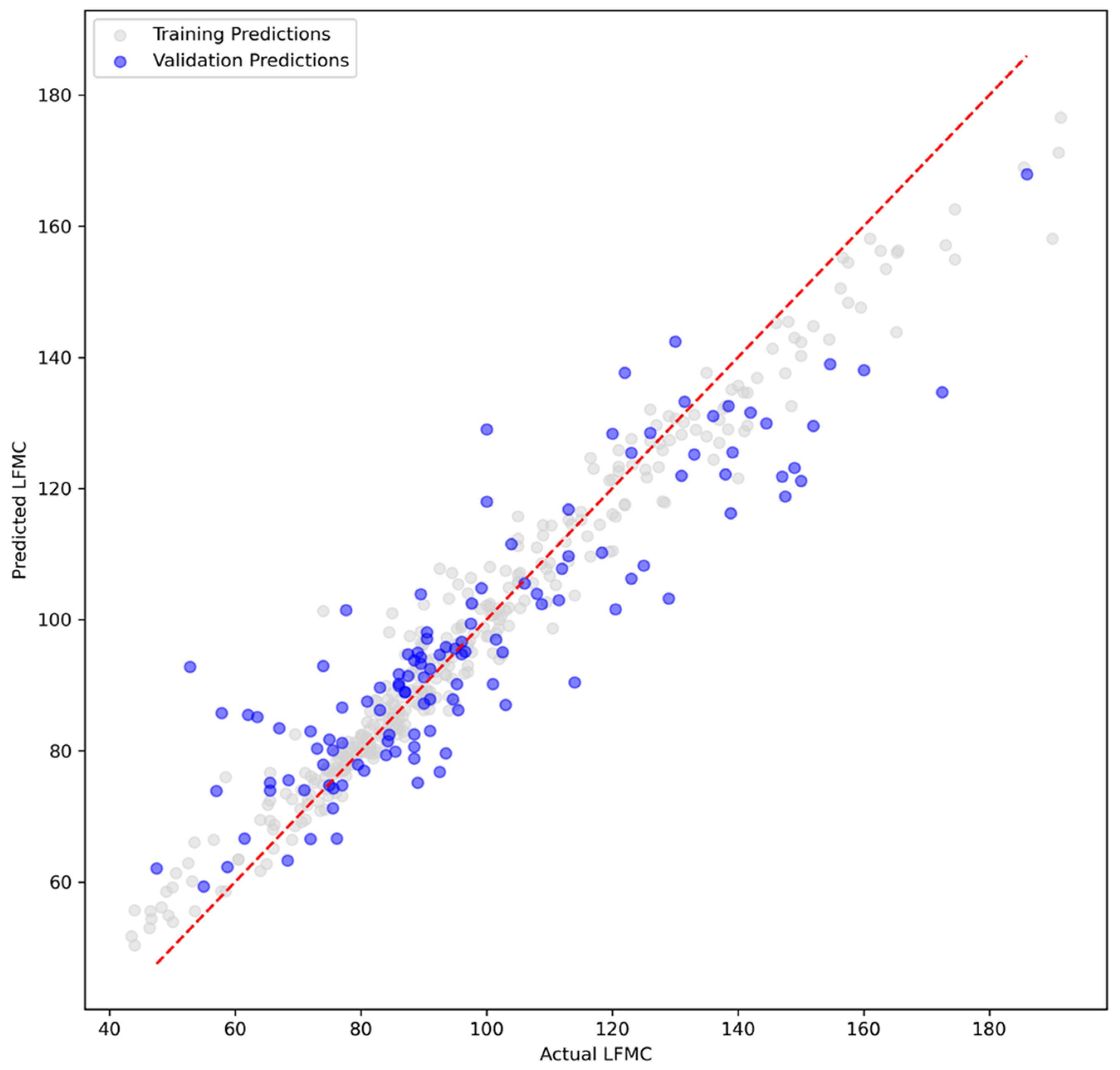
3.1. Global Assessment

Based on the 147 input variables (listed in Table 3), the significant predictors identified through the FFS method were DC, DOY, the 60-day average NDTI, NIR reflectance (band 2), and both the maximum values of NDTI and GVMI (Figure A1, details in Table 3). DC was the most influential predictor with an importance value of approximately 0.35, followed by the DOY at around 0.25, reflecting its role in capturing seasonal cycles. The NDTI60 showed a moderate influence with an importance value of about 0.10. Lower contributions were observed for variables such as NIR reflectance (B2), maximum NDTI (NDTI_max), and maximum GVMI (GVMI_max), each adding specific nuances to the model’s performance.
Figure 2 shows the comparison between sampled and predicted LFMC for the calibration and validation subsets. The performance of the model is high for the calibration subset, as indicated by a high R2 of 0.95, a low RMSE of 6.04% and MAE of 4.14%. For the validation subset, the pairs exhibit a larger dispersion around the 1:1 line, particularly at higher LFMC values. This indicates a lower fit to the data, with a decreased R2 of 0.78 and an increased RMSE and MAE of 12.82% and 9.72%, respectively. These metrics explicitly compare the performance of the model on seen (calibration) and unseen (validation) data, demonstrating an expectable decline in model accuracy when applied to new data. Considering the validation dataset, some underestimation of higher values (LFMC > 140%) was observed, as well as some overestimation of lower values (LFMC < 70%).

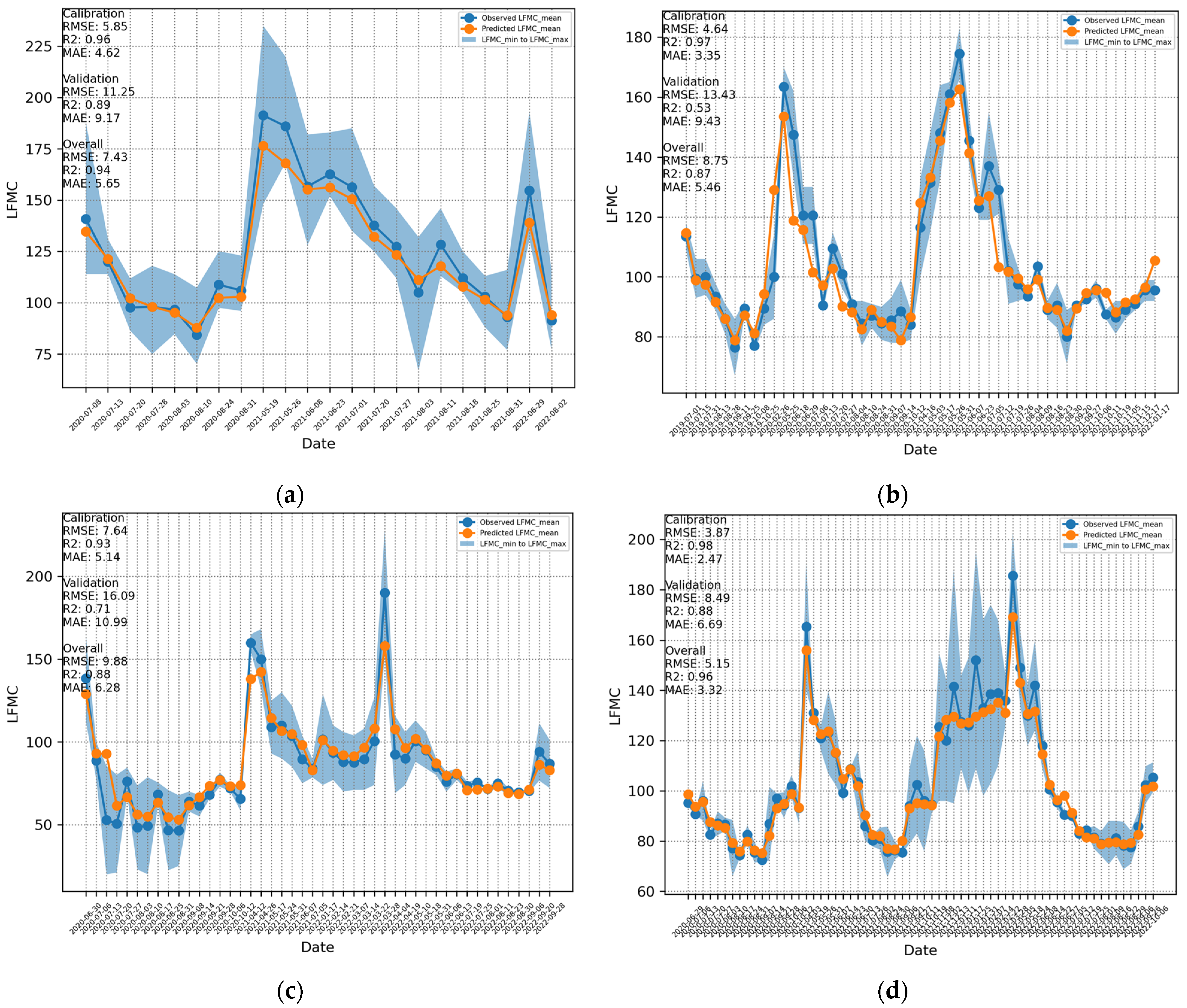
3.2. Site-Level Assessment

Evaluating the performance of LFMC estimates at the sampling sites shows that RMSE values range from 3.06 to 16.43% for the validation dataset and between 1.93 and 10.45% for the entire dataset (Table 4). The R2 ranged between 0.47 and 0.89 for the validation and 0.58 to 0.97 for the entire datasets, respectively. Overall, the results suggest that the model was robust and provided accurate LFMC estimates at site level. No performance differences were found for different sample sizes. For example, the Arrábida site had 46 samples with a validation RMSE of 16.09% and the Monsanto site had an RMSE of 3.06% with a total of 12 samples. Note that, for some of the sampling sites, the validation sample was very small and therefore performance metrics must be addressed with caution. Additionally, no relevant differences in model performance were found for different species composition.
Comparing the time series of observed and predicted LFMC for four different sampling sites shows that the model is capable of capturing the large seasonal LFMC variability (Figure 3). Estimates are in most of the cases within the sampled LFMC variability. Nevertheless, the model tends to underestimate higher LFMC values. In some cases, like in Arrábida—Setúbal (site 2), particularly during the summer of 2020, the model slightly overestimated the significantly low LFMC values observed (lower than 50%). These low values were underrepresented in the full dataset.

3.3. LFMC Mapping

Figure 4 showcases a series of LFMC maps generated using the RF model across mainland Portugal from May to October 2024. The maps illustrate the seasonal evolution of LFMC with higher values in May and June, and lower values in August and September. The maps also show different drying timings, with the southern and northeastern areas drying before the rest of the territory. The northwest is typically the wettest area of Portugal, which can be clearly seen in the maps.
The year of 2024 was particularly wet, with significant rainfall in May and June. Consequently, the fire season started relatively late compared to other years. The first very large wildfires (>500 ha) occurred in mid-August in the northeast of Portugal. In September, over 126,000 ha burned, corresponding to 92% of the total annual burned area. The maps exhibited in Figure 4 are coherent with this narrative, showing the late fuel drying and very low LFMC values during September.
In terms of operational implementation of national-level LFMC maps, the primary limitation is related to the latency of the predictor variables, which varies between 7 to 15 days. This variability in latency primarily stems from the availability of MODIS (MCD43A4) datasets in the GEE catalogs. This latency mostly affects the NIR reflectance (band 2) and the maximum values of NDTI and GVMI.

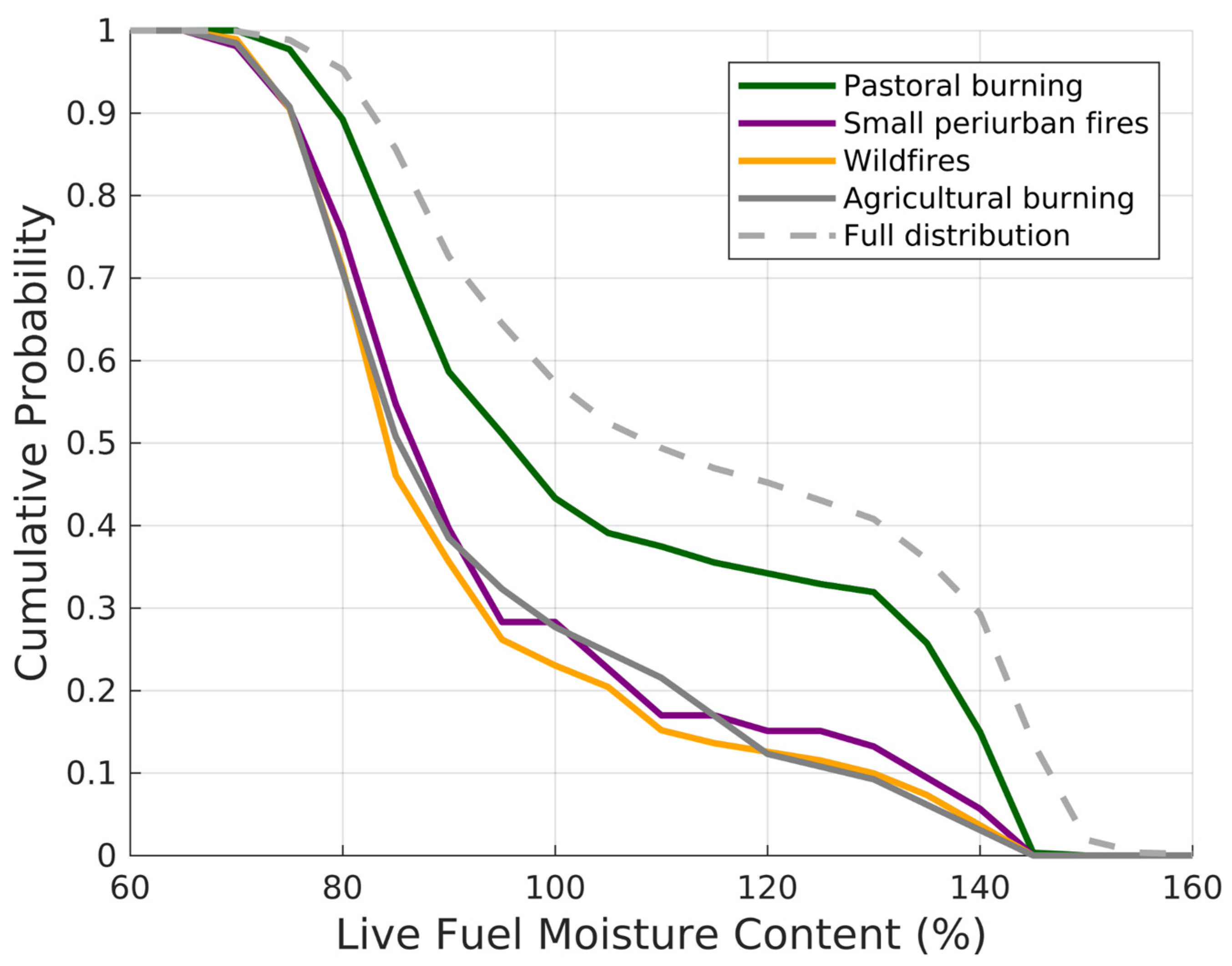
3.4. Relations Between LFMC and Wildfires
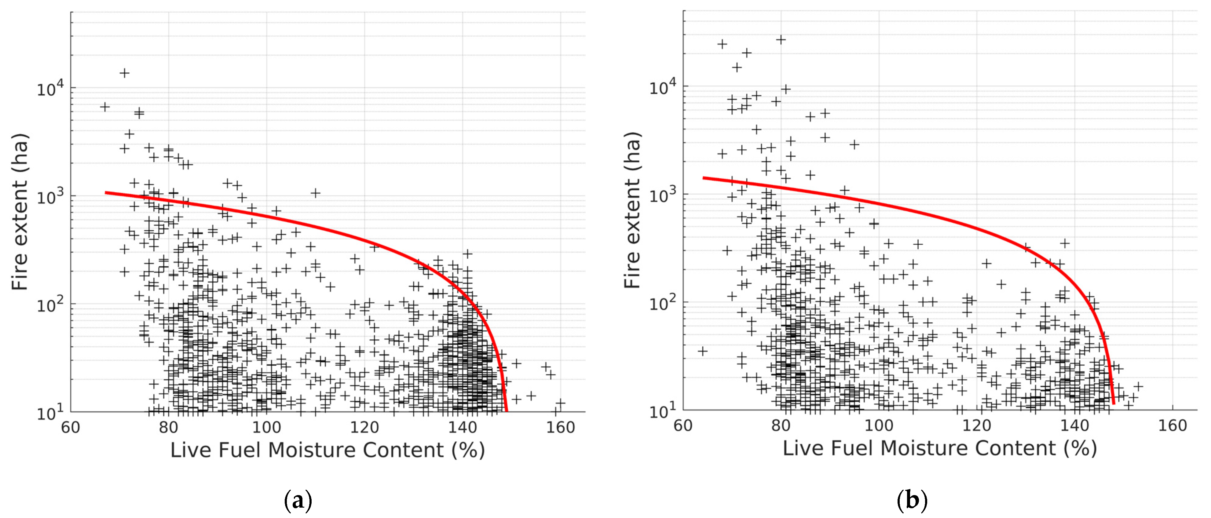
3.4.1. Fire Size

The data show a clear relationship between LFMC and fire size (Figure 5). Larger wildfires tend to occur under drier LFMC conditions and higher LFMC is associated with smaller wildfires. Considering the wildfires larger than 500 ha (N = 103), almost all (98%) occurred with LFMC lower than 100% and 63% occurred with LFMC lower than 80%. Considering the wildfires larger than 1000 ha (N = 59), almost all occurred with LFMC lower than 100% and 70% occurred with LFMC lower than 80%. For the wildfires larger than 5000 ha (N = 19), 84% occurred with LFMC lower than 80%. Results are very similar for both shrub and forest-dominated wildfires (Figure A2).
In Figure 5, a notable fire occurrence peak is evident around LFMC values of 130–150% that corresponds to a total of 51 wildfires with a size larger than 100 ha and a maximum size of 350 ha. All of these wildfires occurred between January and June, and most of them (86%) occurred between January and March, peaking at the latter month (39% of occurrences). Figure 6 shows that these wildfires occur mostly where pastoral burning prevails with around 35% of the large wildfires (>100 ha) occurring with LFMC > 130%. In the remaining fire regimes, the probability distributions are very similar and consistent with the previous result that shows that large wildfires occur mostly in periods of low LFMC. For example, in these three regimes, more than 70 to 80% of the large wildfires (>100 ha) occurred with LFMC < 100%. The probability distribution associated with these regimes is considerably different from the expected probability of the full LFMC distribution (dashed line in Figure 6) and clearly shifted towards lower LFMC values.
The probability distributions for the occurrence of wildfires larger than several different fire size thresholds are displayed in Figure 7. The probability of occurrence of larger wildfires increases with decreasing LFMC, consistent with previous results. Notably, the probability of occurrence of wildfires larger than 5000 ha (N = 19) is constrained to narrow intervals: it is null for LFMC ≥ 90% and increases sharply for lower values, peaking at LFMC of 70%. The probability distributions of wildfires larger than 500 (N = 44) and 1000 ha (N = 40) are similar, with almost all values concentrated in LFMC ≤ 100%. The largest probabilities are concentrated in LFMC values lower than 85%. The probability distributions aforementioned are considerably different from the expected probability of the full LFMC distribution (dashed lines in Figure 7).
The probability distributions of wildfires larger than 50 (N = 276) and 100 ha (N = 278) are similar, with two peaks: one at higher LFMC values, as previously identified, and the other around LFMC of 80%. The probability of the entire LFMC dataset (associated with wildfire occurrence) is also bimodal. A relevant percentage of fires smaller than 50 ha occurs at high LFMC values.
For moist dead and live fuel conditions, most of the wildfires have a small size, typically below 100 ha (Figure 8). No wildfires were observed with DFMC and LFMC above 22% and 150%, respectively. For DFMC values larger than 9%, only five wildfires larger than 1000 ha occurred (~8%), most of them (4/5) coincident with LFMC values lower than 90%. For LFMC values greater than 100%, only one wildfire larger than 1000 ha was observed (1.5%). The larger wildfires clearly tend to occur under a combination of low DFMC and LFMC:
  • Around 90% of wildfires larger than 500 ha occurred for DFMC and LFMC lower than 10% and 100%, respectively;
  • Around 86% of wildfires larger than 1000 ha occurred for DFMC and LFMC lower than 9% and 95%, respectively;
  • Around 84% of wildfires larger than 5000 ha occurred for DFMC and LFMC lower than 8% and 90%, respectively.
Six wildfires stand out from the analysis and the aforementioned thresholds. Three of them occurred with DFMC > 10%, but with LFMC lower than 82%, with the largest wildfire coinciding with an LFMC of 71%. One of the six wildfires occurred with LFMC of 110% but with dry DFMC conditions (<8%).
Figure 8. Scatterplot of the Live versus Dead Fuel Moisture Content (%) for different fire size classes.
Fire 08 00178 g008

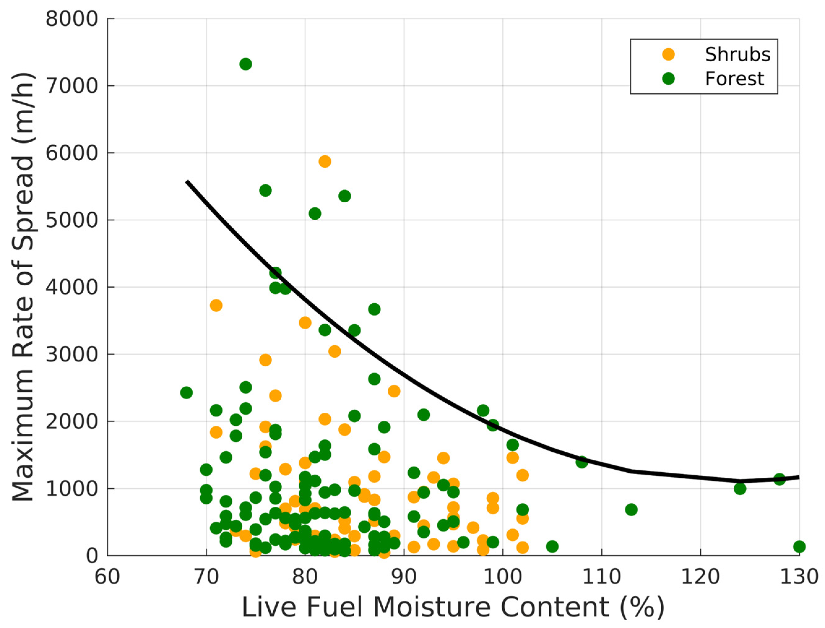
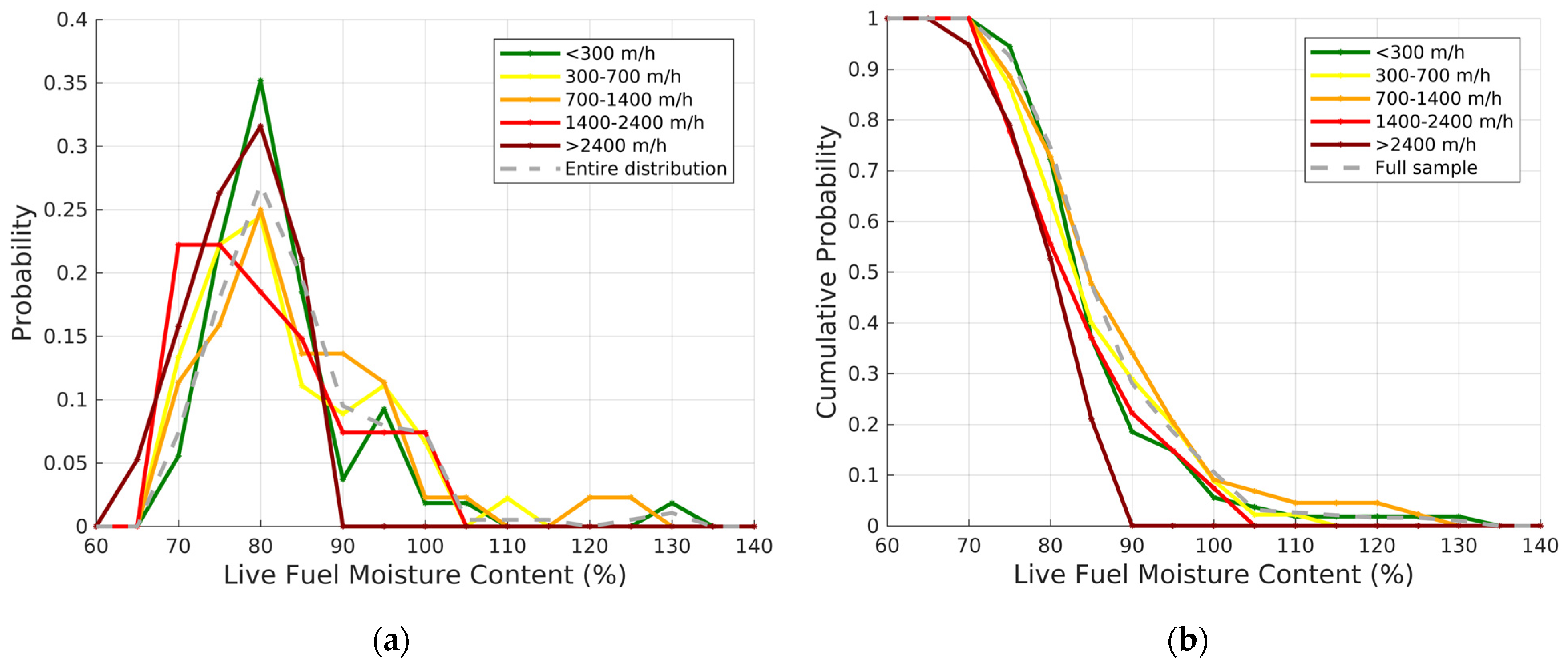
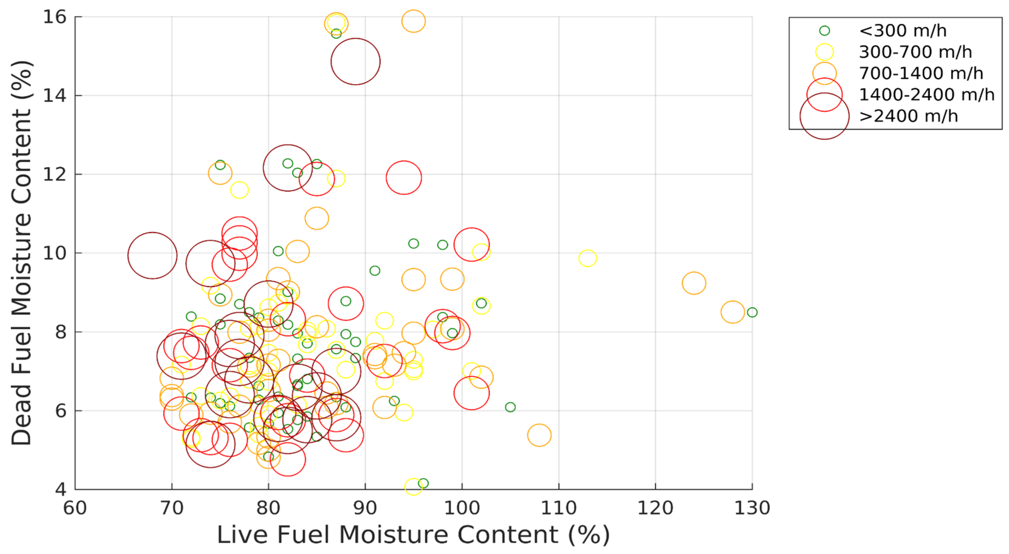
3.4.2. Rate of Spread

Fast-spreading wildfires are coincident with lower LFMC conditions (Figure 9). From a total of 66 observations with ROS larger than 1000 m/h, 92%, 80% and 48% occurred with LFMC values lower than 100%, 90% and 80%, respectively. The steep increase in the slope of the quantile regressions suggests that the conditions associated with low LFMC become a progressively decreasing limit over the maximum ROS.
Maximum ROS observations are mostly concentrated in the 70–100% LFMC range, contrasting with the wider dispersion shown in Figure 5 that includes a broader scope of wildfires that occurred during the entire year. This is particularly evident in the probability distributions for several ROS intervals, since the most important probability peaks occur around LFMC of 80%, regardless of the ROS interval (Figure 10a). The fastest-spreading wildfires (ROS > 2400 m/h) have a higher probability of occurring when LFMC is below 85%, with 80% of the observations occurring below this value (Figure 10b). However, for the remaining ROS classes the distributions are relatively similar.
The maximum ROS observations are also coincident with a relatively low DFMC range, most of them below 12% (Figure 11), adding to the aforementioned low LFMC range. All observations with ROS > 2400 m/h were coincident with LFMC < 90% with DFMC values varying as much as 5 to 15%. Most of these observations (~90%) occurred for low LFMC (<90%) and DFMC (<10%) values. Around 81% of the observations with ROS between 1400 and 2400 m/h occurred for the latter LFMC and DFMC intervals.

4. Discussion

4.1. LFMC Sampling

The importance of the availability of LFMC information to support operational decisions in wildfire seasons has been stated by several authors. This work proposes for the first time a data product of near-real-time (7–15 days latency) mapping for Portugal, in which we need to recognize, nevertheless, some limitations of its applicability. Considering the spatial patterns of Portugal’s climate [57] and fire regime [55], the spatial distribution LFMC sampling sites can be considered representative of the North and parts of the Center region, although some relevant gaps exist in the latter. The most relevant limitation is the coverage over southern Portugal, in particular, the lack of samples in the southernmost fire-prone region of Algarve.
This sampling limitation may affect LFMC modeling and the degree to which it is representative of the entire country, with impact in the local model’s accuracy due to unrepresented variability in vegetation and climate conditions. To mitigate these issues, we employed a RF model which is robust against such disparities by ensembling multiple decision trees, thus diminishing the influence of any single over-represented area. RF’s ability to handle complex, high-dimensional datasets, including varied climatic and land cover inputs, helps counterbalance the spatial biases and enhances the reliability of predictions across all areas, including those less represented like the south of Portugal. Results showed that for southern Portugal, the relations between LFMC and fire size are consistent with the results for the entire country (Figure A3), strengthening our confidence in the extrapolation of the LFMC model to underrepresented areas.

4.2. LFMC Modelling

The LFMC model had a global R2 of 0.78 and a RMSE of 12.82%, ranging between 3.06 to 16.43% when evaluated for the different sampling sites. The RMSE values attained are within the range reported in other studies such as Ruffault et al. [58], which documented RMSE values for different models ranging between 13.54% and 18.36%. Marino et al. [28] highlighted challenges in modeling LFMC with an RMSE of 15.05% using the MCD43A4 product. Tanase et al. [36] used static variables and Sentinel-2 imagery in the Madrid region, reporting a RF model performance with an R2 of 0.55 that improved to 0.63, when combined with static variables. Cunill Camprubí et al. [30] reported an RMSE range of 16–20% across the Western Mediterranean using RF models. Zhu et al. [35] reported an R2 of 0.7 with an RMSE of 8.13% for LFMC modeling in the Valencia region. Overall, the results suggest our models are robust, when compared to a variety of other studies, affirming their validity for practical applications in wildfire risk assessment.
The model is capable of capturing the seasonal LFMC variability, from higher values in the winter to lower values in late summer. The model tends to slightly overestimate very low LFMC values, which can be problematic for operational purposes. This is mainly caused by the severe underrepresentation of very low sampled LFMC values. The challenges in estimating these low values, as highlighted by Marino et al. [28], signal an important need to enhance predictive models. Such improvements are necessary to ensure reliable identification of conditions related with a heightened risk of wildfire, contributing to more effective fire risk mitigation and management strategies.
The model is also capable of capturing the spatial variability that is coherent with the arid–wet contrasts present over mainland Portugal [57]. This variability is also clear in the different drying timings, with the more arid areas of the south and northeast drying before the rest of the territory. Considering the absence of LFMC samples in the south of Portugal (as discussed in Section 4.1), LFMC estimates over this area should be used cautiously. Nevertheless, the LFMC maps (Figure 5) show that this area is drier than most of the rest of the country, which is coherent with its known climate and occurrence of several very large wildfires in recent decades.
Despite the noteworthy efforts made by national authorities in systematically collecting LFMC data across the country, the sampling dataset is still relatively small. In comparison with other studies, our sample set is larger than the one used by Costa-Saura et al. [29], similar to the one used by Lai et al. [33], and smaller than the ones used by several other studies [30,31,35,36,58]. This not only affects the modelling approach, but mostly the validation statistics that in some cases are computed over a very low number of observations for some sampling sites. Regardless, the global validation statistics were calculated over 120 observations and can be considered reliable, agreeing well between estimated and observed LFMC.
LFMC has been mostly estimated using statistical or radiative transfer modelling (RTM) techniques [28,32]. Some authors have shown that RF (as well as other machine learning methods) can be used to model LFMC with high accuracy, in some cases surpassing conventional techniques [30,34]. Most importantly, we showed that RF can provide LFMC estimates that have an accuracy fit for the purpose. LFMC has been estimated with resolutions ranging from 10 m [29] to 9 km [59], although most are within the 250 m–500 m range [30,31,34,60]. Our LFMC estimates have 500 m spatial resolution that enables detailed information to perform both national-level fire danger assessment (Figure 4), as well as landscape-level fire behavior assessment. Evidence suggests higher-resolution estimates do not lead to substantial model performance increase [28]. Some authors have produced higher-resolution estimates with lower frequency that limits operational application [31,60]. We showed that 500 m weekly LFMC estimates are suitable for real-time operational applications.
Most importantly, most of the studies do not provide near-real-time LFMC estimates and/or do not develop their models using data that can be used in near-real time with the same model accuracy. A noteworthy exception is the Australian Flammability Monitoring System (http://wenfo.org/afms, accessed on 1 March 2025) that provides daily LFMC estimates for Australia based on the work of Yebra et al. [32]. Camprubi et al. [30] created LFMC estimates for the Mediterranean basin between 2001 and 2021; however, they did not provide real-time estimates. Our work fills the gap by providing accurate LFMC maps for the entire mainland territory of Portugal at a spatial and temporal resolution suitable for real-time operational awareness and decision-making. However, the latency of the predictor variables could hinder its application. The latency of the MODIS data varies between 7 and 15 days. Although LFMC variation is relatively slow over time, high latencies can lead to the inability to anticipate increased fire danger due to steep LFMC decreases. Potential improvements to minimize this limitation are addressed in Section 4.4.

4.3. Relations Between LFMC and Wildfires

In this work, we compared the LFMC estimates with the size of individual wildfires and the maximum ROS to evaluate whether LFMC could be used as an indicator of increased fire danger and a driver of fire behavior. For operational purposes, it is important that LFMC estimates are well-correlated with both, ensuring that these can be used for fire management in an operational context.

4.3.1. Fire Size

Overall, the LFMC estimates can be considered a good proxy for identifying the potential occurrence of large wildfires in the Portuguese mainland territory. There is a clear relation between LFMC and fire size with results showing that larger wildfires occur under lower LFMC values. In particular, a large fraction of wildfires larger than 1000 and 5000 ha occurred with LFMC lower than 80%, demonstrating that LFMC can be used to define fire danger in an operational context [6]. Previous studies have reported a threshold of shrub LFMC associated with large wildfires that varies between 80% and 105% [6,9,10,11,26]. The range of thresholds depends, among other factors, on the statistical methodologies employed, shrub species and the large fire threshold. Our results are consistent with the range of reported LFMC thresholds, reinforcing the idea that large wildfires occur when the availability of vegetation to burn “switch” is activated along with the remaining “switches” [1].
A prominent fire peak was evident for high LFMC corresponding to winter and early spring wildfires. This peak is associated with pastoral burning concentrated in specific mountainous areas in the north and center of Portugal [55]. These latter conditions are not captured in the LFMC estimates, possibly due to the strong anthropogenic influence exerted on these wildfires. Additionally, the lower level of seasonal firefighting preparedness allows wildfire growth irrespective of the existence of potential barriers for fire spread [61]. These winter and early spring wildfires have a small relative contribution to the total annual burned area when compared with summer wildfires [62], and are not a concern for operational purposes. Other authors have reported high pre-fire moisture conditions, underlining that LFMC is only one of the variables that needs to be considered [12,32].
The control of fuel moisture over wildfire size was clear. For both high DFMC and/or high LFMC, wildfire size is limited. For drier conditions, the occurrence of large wildfires is more likely, as shown by the fact that 90% of the wildfires larger than 500 ha occurred with DFMC and LFMC lower than 10% and 100%, respectively. Very large wildfires mostly occurred with DFMC and LFMC lower than 8% and 90%, respectively. The results come as no surprise since the combination of dead and live fuel moisture is one of the key aspects of the US National Fire Danger Rating System [13]. Similar to the previously discussed LFMC thresholds, these results show that one of the four fire “switches” [1] is activated when DFMC and LFMC are close to or below certain thresholds.

4.3.2. Rate of Spread

Fuel dryness is just one of the many environmental drivers of fire behavior. Fast-spreading wildfires occurred mostly under LFMC below 100%, consistent with the findings of Pimont et al. [9]. Around 80% of the wildfires that had ROS larger than 1000 m/h occurred under LFMC lower than 90%. There was a clear and steep increase in the slope of the quantile regressions for decreasing LFMC. This result further supports the claims of Pimont et al. [9] that the LFMC effect on ROS is larger than previously reported by Anderson et al. [15], particularly when using a large sample with an LFMC range consistent with typical Mediterranean conditions.
Most ROS observations corresponded with relatively low LFMC values due to the very low frequency of large wildfires and lower fire spread monitoring capacity [54] outside of the fire season when LFMC is typically higher. The lower range of LFMC values cannot be considered a limitation due to the reasons presented by Pimont et al. [9].
LFMC may respond differently to its drivers depending on plant functional type [63], and the effect of LFMC on fire behavior should vary with the ratio of dead-to-live fuel [64]. Nonetheless, the relations between maximum ROS and LFMC for both shrublands and forests were similar. These results provide added confidence on extrapolating the LFMC model to forested areas. Nevertheless, additional observations of shrub LFMC in forests are necessary in the future to ensure that the model is robust over these areas.
Maximum ROS observations were mostly concentrated in the 70–100% LFMC range, contrasting with the wider dispersion shown in Figure 6 that includes a broader scope of wildfires that occurred during the entire year. This is particularly evident in the probability distributions for several ROS intervals, since the most important probability peaks occur around LFMC of 80%, regardless of the ROS interval (Figure 10a). The fastest-spreading wildfires (ROS > 2400 m/h) have a higher probability of occurring when LFMC is below 85%, with 80% of the observations occurring below this value (Figure 10b). However, for the remaining ROS classes the distributions are relatively similar. Due to the concentration of observations over a relatively narrow LFMC range and to the similarity between the LFMC distributions for several ROS classes, any further conclusions must be addressed cautiously. The fastest ROS observations occurred for LFMC < 90% and DFMC < 10%. The five fastest wildfires (ROS > 5000 m/h) occurred with LFMC ~ 80% and DFMC ~ 6%, respectively. It is noteworthy to mention that not only ROS depends on factors other than FMC; the results show a correlation between DFMC and LFMC (Figure 11), as shown by Rossa and Fernandes [65], and therefore the individual contributions to ROS are difficult to disentangle.

4.4. Future Improvements

Despite the good results and the creation of an unprecedented dataset in Portugal, several improvements are needed to create more robust LFMC estimates in the future and maximize their usefulness for fire management.
The national authorities made a notable effort in collecting more than 1000 samples of LFMC across diverse landscapes in Portugal. Nevertheless, it is important that this effort is maintained over time, particularly in the most relevant locations. The number of sampling sites could be reduced as long as it is ensured that these provide representative measurements over relatively large areas. The LFMC estimates can be used to identify these locations, combined with correlation analysis between different sampling sites whenever possible. It is very important to add sampling sites to the south of Portugal, in particular the fire-prone region of Algarve, and to collect LFMC samples under extreme conditions to improve the model’s ability to represent very dry conditions.
We used a very large set of predictor variables, although limited to those that were available in an operational context. For these reasons, we did not use the ERA5-Land hourly data which contain important weather, soil and vegetation-related parameters [66]. With expectable decreased latency times in the future, ERA5-Land data could be used to create an improved LFMC model, with the added advantage of enabling an extrapolation to years prior to 2018. In particular, soil moisture has been shown to have a good relation with LFMC [27] and could entail promising improvements. Other datasets that can be exploited are Sentinel-2 reflectances and derived vegetation indices [29], as well as the Fire Risk Map (FRM), that contains the FWI sub-indices forecasted using ECMWF weather forecasts [67], minimizing the impact of interpolation errors from station data [58]. Particular attention should be paid to reducing latency time, which can be done by, for example, narrowing down the potential predictor variables. One important limitation is that the model relies on data from MODIS, which will be decommissioned in the near future. The best candidate to replace MODIS is likely to be the Visible Infrared Imaging Radiometer Suite (VIIRS) due to similar sensor characteristics [68].
A more detailed analysis is required to better understand the role of LFMC in driving the size and behavior of wildfires. An important future step would be to apply the LFMC model to a much larger time period which would require using other input variables (e.g., ERA-5). The limitations of using daily DFMC data were highlighted previously. To account for confounded effects, future work should use weather (e.g., wind speed) and other environmental variables (e.g., topography) adequately correlated to the location and duration of the more relevant burning periods. For multi-day wildfires, this could be a challenging task that should be pursued at least for the wildfires contained in the PT-FireSprd database [54].

5. Conclusions

We developed a robust model capable of estimating near-real-time LFMC across Portugal, with an R2 of 0.78 and an RMSE of 12.82%, with performance statistics better than or comparable with similar studies. The LFMC maps are produced every week with a spatial resolution of 500 m, adequate for operational purposes. The model captures well both the spatial and temporal variability of LFMC, although estimates for very dry periods and the south of Portugal must be addressed with caution due to the underrepresentation of both in the sampling dataset.
The comparison of LFMC with fire size showed that larger wildfires typically occur under low LFMC conditions, whereas high LFMC constrains fire size. Most of the largest wildfires occurred with LFMC below 80% and there was a clear tipping point around LFMC of 100%. Relations with maximum ROS were not as clear as with fire size; however, the fastest-spreading wildfires occurred mostly with LFMC < 85%.
Future improvements should focus (at least) on extending LFMC sampling to the south of Portugal, improving the model’s capability to predict very low LFMC values and use additional variables with recognized added value (e.g., ERA5-Land). For operational purposes, it is very important that data latency is reduced to minimal values.
Spatial and temporal LFMC variability for Portugal was unavailable up to now. Weekly LFMC maps are available at https://pccir.isa.ulisboa.pt/portal/apps/sites/#/pccir, accessed on 1 March 2024 (see “Humidade Combustíveis Vivos”) in near-real time and the 2018–2024 dataset is available for download. We expect that this new piece of information will not only be relevant for better fire management decision-making, by improving the anticipation of the occurrence of large and fast-spreading wildfires, but also will allow a better understanding of the drivers of large wildfires.

Author Contributions

Conceptualization, A.B. and F.B.; methodology, A.B., C.L., G.B. and R.F.; formal analysis, A.B., G.B. and R.F.; writing—original draft preparation, A.B., G.B. and R.F.; writing—review, A.B., G.B., C.L., F.B., P.M.F., C.R. and R.F. All authors have read and agreed to the published version of the manuscript.

Funding

This research was funded by project FUELSAT (PCIF/GRF/0116/2019) funded by the Fundação para a Ciência e a Tecnologia I.P. (FCT). The Forest Research Centre was funded by FCT (UIDB/00239, Centro de Estudos Florestais). AB was funded by FCT through a CEEC contract (CEECIND/03799/2018/CP1563/CT0003). P.M.F and C.R. were supported by FCT under the projects UID/04033: Centro de Investigação e de Tecnologias Agro-Ambienteis e Biológicas and LA/P/0126/2020 (https://doi.org/10.54499/LA/P/0126/2020).

Institutional Review Board Statement

Not applicable.

Informed Consent Statement

Not applicable.

Data Availability Statement

The LFMC dataset for the period 2018–2024 is available for download here: https://zenodo.org/records/14983462, accessed on 1 March 2025. The near-real-time LFMC estimates are available at https://pccir.isa.ulisboa.pt/portal/apps/sites/#/pccir, accessed on 1 March 2025 (see “Humidade Combustíveis Vivos”).

Acknowledgments

We thank AGIF and ICNF for collecting LFMC samples and openly sharing the data. We thank Yannick Le Page for help with the sampled LFMC data and Carlos Mota for integrating the LFMC model to produce near-real-time estimates in an open WEB-GIS.

Conflicts of Interest

The authors declare no conflicts of interest.

Abbreviations

The following abbreviations are used in this manuscript:
FMCFuel Moisture Content
LFMCLive Fuel Moisture Content
DFMCDead Fuel Moisture Content
ROSRate of spread
FWIFire Weather Index
AGIFAgency for Integrated Management of Rural Fires
ICNFInstitute for Forest and Nature Conservation
GEEGoogle Earth Engine
MODISModerate Resolution Imaging Spectroradiometer
SIVegetation Spectral Indices
LSTLand Surface Temperature
DCDrought Code
FFMCFine Fuel Moisture Code
DOYDay of year
RFRandom Forests
RMSERoot Mean Square Error
MAEMean absolute error

Appendix A

This appendix presents additional information on the hyperparameters used in the Random Forest Model (Table A1).
Table A1. Hyperparameters used for fine-tuning the Random Forest model using a grid search approach.
ParameterDescriptionValues
n_estimatorstotal number of trees10, 25, 50, 100, 250, 300, 350, 400, 450, 500
max_featuresnumber of variables (or features) randomly selected at each split‘sqrt’, ‘log2’
max_depthmaximum number of levels in each decision tree7, 8, 9, 10, 11, 12, 13, 14, 15, 16, 17, 18, 19, None

Appendix B

This appendix presents additional analysis of the importance of the main LFMC model predictor variables (Figure A1), LFMC and fire size comparison for shrub- and forest-dominated wildfires (Figure A2), and LFMC and fire size comparison for the south of Portugal (Figure A3).
Figure A1. Feature importance analysis detailing the relative importance of each variable in predicting LFMC in vegetation. The Y-axis displays the calculated feature importance scores for each variable.
Fire 08 00178 g0a1
Figure A2. Scatterplot of LFMC (%) against fire size (ha) for shrub- (a) and forest-dominated (b) wildfires. Each black cross represents a wildfire. The red lines represent the quantile regressions.
Fire 08 00178 g0a2
Figure A3. Scatterplot of LFMC (%) against fire size (ha) considering only wildfires that occurred in the south of Portugal (latitude between 36.9 and 38.3°). Each black cross represents a wildfire. The red line represents the quantile regression.
Fire 08 00178 g0a3

References

  1. Bradstock, R.A. A biogeographic model of fire regimes in Australia: Current and future implications. Glob. Ecol. Biogeogr. 2010, 19, 145–158. [Google Scholar] [CrossRef]
  2. Jolly, W.M. Sensitivity of a surface fire spread model and associated fire behaviour fuel models to changes in live fuel moisture. Int. J. Wildland Fire 2007, 16, 503–509. [Google Scholar] [CrossRef]
  3. Nelson, R.M. Water relations of forest fuels. In Forest Fires: Behavior and Ecological Effects; Johnson, E.A., Miyanishi, K., Eds.; Academic Press: San Diego, CA, USA, 2001; pp. 79–149. [Google Scholar]
  4. Jolly, W.M.; Johnson, D.M. Pyro-ecophysiology: Shifting the paradigm of live wildland fuel research. Fire 2018, 1, 8. [Google Scholar] [CrossRef]
  5. Rodrigues, M.; de Dios, V.R.; Sil, Â.; Camprubí, A.C.; Fernandes, P.M. VPD-based models of dead fine fuel moisture provide best estimates in a global dataset. Agric. For. Meteorol. 2024, 346, 109868. [Google Scholar] [CrossRef]
  6. Jurdao, S.; Chuvieco, E.; Arevalillo, J.M. Modelling fire ignition probability from satellite estimates of live fuel moisture content. Fire Ecol. 2012, 8, 77–97. [Google Scholar] [CrossRef]
  7. Viegas, D.X.; Viegas, M.; Ferreira, A.D. Moisture content of fine forest fuels and fire occurrence in central Portugal. Int. J. Wildland Fire 1992, 2, 69–86. [Google Scholar] [CrossRef]
  8. Rossa, C.G. The effect of fuel moisture content on the spread rate of forest fires in the absence of wind or slope. Int. J. Wildland Fire 2017, 26, 24. [Google Scholar] [CrossRef]
  9. Pimont, F.; Ruffault, J.; Martin-StPaul, N.K.; Dupuy, J.L. Why is the effect of live fuel moisture content on fire rate of spread underestimated in field experiments in shrublands? Int. J. Wildland Fire 2019, 28, 127–137. [Google Scholar] [CrossRef]
  10. Dennison, P.E.; Moritz, M.A. Critical live fuel moisture in chaparral ecosystems: A threshold for fire activity and its relationship to antecedent precipitation. Int. J. Wildland Fire 2009, 18, 1021–1027. [Google Scholar] [CrossRef]
  11. Nolan, R.H.; Boer, M.M.; Resco de Dios, V.; Caccamo, G.; Bradstock, R.A. Large-scale, dynamic transformations in fuel moisture drive wildfire activity across southeastern Australia. Geophys. Res. Lett. 2016, 43, 4229–4238. [Google Scholar] [CrossRef]
  12. Luo, K.; Quan, X.; He, B.; Yebra, M. Effects of live fuel moisture content on wildfire occurrence in fire-prone regions over southwest China. Forests 2019, 10, 887. [Google Scholar] [CrossRef]
  13. Jolly, W.M.; Freeborn, P.H.; Bradshaw, L.S.; Wallace, J.; Brittain, S. Modernizing the US National Fire Danger Rating System (version 4): Simplified fuel models and improved live and dead fuel moisture calculations. Environ. Model. Softw. 2024, 181, 106181. [Google Scholar] [CrossRef]
  14. Alexander, M.E.; Cruz, M.G. Assessing the effect of foliar moisture content on the spread rate of crown fires. Int. J. Wildland Fire 2013, 22, 415–427. [Google Scholar] [CrossRef]
  15. Anderson, W.R.; Cruz, M.G.; Fernandes, P.M.; McCaw, L.; Vega, J.A.; Bradstock, R.A.; Fogarty, L.; Gould, J.; McCarthy, G.; Marsden-Smedley, J.B.; et al. A generic, empirical-based model for predicting rate of fire spread in shrublands. Int. J. Wildland Fire 2015, 24, 443–460. [Google Scholar] [CrossRef]
  16. Marino, E.; Dupuy, J.L.; Pimont, F.; Guijarro, M.; Hernando, C.; Linn, R. Fuel bulk density and fuel moisture content effect on fire rate of spread: A comparison between FIRETEC model predictions and experimental results in shrub fuels. J. Fire Sci. 2012, 30, 277–299. [Google Scholar] [CrossRef]
  17. Rossa, C.G.; Fernandes, P.M. Live fuel moisture content: The ‘pea under the mattress’ of fire spread rate modeling? Fire 2018, 1, 43. [Google Scholar] [CrossRef]
  18. Yebra, M.; Dennison, P.E.; Chuvieco, E.; Riaño, D.; Zylstra, P.; Hunt, E.R., Jr.; Jurdao, S. A global review of remote sensing of live fuel moisture content for fire danger assessment: Moving towards operational products. Remote Sens. Environ. 2013, 136, 455–468. [Google Scholar] [CrossRef]
  19. van Wagner, C.E.; Stocks, B.J.; Lawson, B.D.; Alexander, M.E.; Lynham, T.J.; McAlpine, R.S. Development and Structure of the Canadian Forest Fire Behavior Prediction System; Fire Danger Group, Forestry Canada: Ottawa, ON, Canada, 1992. [Google Scholar]
  20. Finney, M.A. FARSITE, Fire Area Simulator—Model Development and Evaluation (No. 4); U.S. Department of Agriculture, Forest Service, Rocky Mountain Research Station: Fort Collins, CO, USA, 1998.
  21. Rothermel, R.C. A Mathematical Model for Predicting Fire Spread in Wildland Fuels; Intermountain Forest & Range Experiment Station, Forest Service, U.S. Department of Agriculture: Fort Collins, CO, USA, 1972; Volume 115. [Google Scholar]
  22. Rossa, C.G.; Fernandes, P.M. Empirical modeling of fire spread rate in no-wind and no-slope conditions. For. Sci. 2018, 64, 358–370. [Google Scholar] [CrossRef]
  23. Matthews, S. Effect of drying temperature on fuel moisture content measurements. Int. J. Wildland Fire 2010, 19, 800–802. [Google Scholar] [CrossRef]
  24. Rossa, C.G.; Fernandes, P.M.; Pinto, A. Measuring foliar moisture content with a moisture analyzer. Can. J. For. Res. 2015, 45, 776–781. [Google Scholar] [CrossRef]
  25. Caccamo, G.; Chisholm, L.A.; Bradstock, R.A.; Puotinen, M.L.; Pippen, B.G. Monitoring live fuel moisture content of heathland, shrubland and sclerophyll forest in south-eastern Australia using MODIS data. Int. J. Wildland Fire 2011, 21, 257–269. [Google Scholar] [CrossRef]
  26. Pellizzaro, G.; Cesaraccio, C.; Duce, P.; Ventura, A.; Zara, P. Relationships between seasonal patterns of live fuel moisture and meteorological drought indices for mediterranean shrubland species. Int. J. Wildland Fire 2007, 16, 232–241. [Google Scholar] [CrossRef]
  27. Vinodkumar, V.; Dharssi, I.; Yebra, M.; Fox-Hughes, P. Continental-scale prediction of live fuel moisture content using soil moisture information. Agric. For. Meteorol. 2021, 307, 108503. [Google Scholar] [CrossRef]
  28. Marino, E.; Yebra, M.; Guillén-Climent, M.; Algeet, N.; Tomé, J.L.; Madrigal, J.; Guijarro, M.; Hernando, C. Investigating live fuel moisture content estimation in fire-prone shrubland from remote sensing using empirical modelling and RTM simulations. Remote Sens. 2020, 12, 2251. [Google Scholar] [CrossRef]
  29. Costa-Saura, J.M.; Balaguer-Beser, Á.; Ruiz, L.A.; Pardo-Pascual, J.E.; Soriano-Sancho, J.L. Empirical models for spatio-temporal live fuel moisture content estimation in mixed Mediterranean vegetation areas using Sentinel-2 indices and meteorological data. Remote Sens. 2021, 13, 3726. [Google Scholar] [CrossRef]
  30. Cunill Camprubi, A.; González-Moreno, P.; Resco de Dios, V. Live fuel moisture content mapping in the Mediterranean Basin using random forests and combining MODIS spectral and thermal data. Remote Sens. 2022, 14, 3162. [Google Scholar] [CrossRef]
  31. Xie, J.; Qi, T.; Hu, W.; Huang, H.; Chen, B.; Zhang, J. Retrieval of live fuel moisture content based on multi-source remote sensing data and ensemble deep learning model. Remote Sens. 2022, 14, 4378. [Google Scholar] [CrossRef]
  32. Yebra, M.; Quan, X.; Riaño, D.; Larraondo, P.R.; Dijk, A.I.J.M.V.; Cary, G.J. A fuel moisture content and flammability monitoring methodology for continental Australia based on optical remote sensing. Remote Sens. Environ. 2018, 212, 260–272. [Google Scholar] [CrossRef]
  33. Lai, G.; Quan, X.; Yebra, M.; He, B. Model-driven estimation of closed and open shrublands live fuel moisture content. GIScience Remote Sens. 2022, 59, 1837–1856. [Google Scholar] [CrossRef]
  34. Quan, X.; Yebra, M.; Riaño, D.; He, B.; Lai, G.; Liu, X. Global fuel moisture content mapping from MODIS. Int. J. Appl. Earth Obs. Geoinf. 2021, 101, 102354. [Google Scholar] [CrossRef]
  35. Zhu, L.; Webb, G.I.; Yebra, M.; Scortechini, G.; Miller, L.; Petitjean, F. Live fuel moisture content estimation from MODIS: A deep learning approach. ISPRS J. Photogramm. Remote Sens. 2021, 179, 81–91. [Google Scholar] [CrossRef]
  36. Tanase, M.A.; Nova, J.P.G.; Marino, E.; Aponte, C.; Tomé, J.L.; Yáñez, L.; Madrigal, J.; Guijarro, M.; Hernando, C. Characterizing live fuel moisture content from active and passive sensors in a Mediterranean environment. Forests 2022, 13, 1846. [Google Scholar] [CrossRef]
  37. Gorelick, N.; Hancher, M.; Dixon, M.; Ilyushchenko, S.; Thau, D.; Moore, R. Google Earth Engine: Planetary-scale geospatial analysis for everyone. Remote Sens. Environ. 2017, 202, 18–27. [Google Scholar] [CrossRef]
  38. Schaaf, C.; Wang, Z. MCD43A4 MODIS/Terra+ Aqua BRDF/Albedo Nadir BRDF-Adjusted Ref Daily L3 Global 500m V006. NASA EOSDIS L. Process. DAAC; United States Geological Survey: Sioux Falls, SD, USA, 2015.
  39. Wan, Z.; Zhang, Y.; Zhang, Q.; Li, Z. Validation of the land-surface temperature products retrieved from Terra Moderate Resolution Imaging Spectroradiometer data. Remote Sens. Environ. 2015, 83, 163–180. [Google Scholar] [CrossRef]
  40. Carroll, M.L.; Townshend, J.R.G.; Hansen, M.C.; DiMiceli, C.M.; Huang, R.A.; Townshend, C. User guide for the MODIS Vegetation Continuous Fields Product, Collection 6, Version 1. 2017. Available online: https://lpdaac.usgs.gov/sites/default/files/public/product_documentation/mod44b_user_guide_v6.pdf (accessed on 1 March 2024).
  41. Buchhorn, M.; Smets, B.; Bertels, L.; Lesiv, M.; Tsendbazar, N.-E.; Herold, M.; Fritz, S. Copernicus Global Land Service: Land Cover 100m: Collection 3: Epoch 2019: Globe; Zenodo: Geneva, Switzerland, 2020. [Google Scholar] [CrossRef]
  42. Farr, T.G.; Rosen, P.A.; Caro, E.; Crippen, R.; Duren, R.; Hensley, S.; Alsdorf, D. The Shuttle Radar Topography Mission. Rev. Geophys. 2007, 45, RG2004. [Google Scholar] [CrossRef]
  43. Theobald, D.M.; Harrison-Atlas, D.; Monahan, W.B.; Albano, C.M. Ecologically-relevant maps of landforms and physiographic diversity for climate adaptation planning. PLoS ONE 2015, 10, e0143619. [Google Scholar] [CrossRef]
  44. Van Wagner, C.E. Development and Structure of the Canadian Forest Fire Weather Index System; Forestry Canadian Forestry Service: Ottawa, ON, USA, 1987. [Google Scholar]
  45. Instituto Português do Mar e da Atmosfera (IPMA). Nota Metodológica para o Cálculo do Índice de Risco de Incêndio Rural. 2020. [Online]. Available online: http://www.ipma.pt (accessed on 1 March 2024).
  46. Breiman, L. Random forests. Mach. Learn. 2001, 45, 5–32. [Google Scholar] [CrossRef]
  47. Kuhn, M.; Johnson, K. Applied Predictive Modeling; Springer: Berlin/Heidelberg, Germany, 2013. [Google Scholar]
  48. Krstajic, D.; Buturovic, L.J.; Leahy, D.E.; Thomas, S. Cross-validation pitfalls when selecting and assessing regression and classification models. J. Cheminform. 2014, 6, 10. [Google Scholar] [CrossRef]
  49. Meyer, H.; Reudenbach, C.; Hengl, T.; Katurji, M.; Nauss, T. Improving performance of spatio-temporal machine learning models using forward feature selection and target-oriented validation. Environ. Model. Softw. 2018, 101, 1–9. [Google Scholar] [CrossRef]
  50. Guyon, I.; Elisseeff, A. An introduction to variable and feature selection. J. Mach. Learn. Res. 2003, 3, 1157–1182. [Google Scholar]
  51. Li, X.; Zhang, Y.; Wang, Z. A comparative analysis of resampling methods in remote sensing. Remote Sens. 2022, 14, 456. [Google Scholar]
  52. Direção Geral do Território. Portuguese Land Cover and Land Use Map for 2018. Available online: https://www.dgterritorio.gov.pt/Carta-de-Uso-e-Ocupacao-do-Solo-para-2018 (accessed on 5 January 2025).
  53. Sá, A.C.L.; Benali, A.; Aparicio, B.A.; Bruni, C.; Mota, C.; Pereira, J.M.C.; Fernandes, P.M. A method to produce a flexible and customized fuel models dataset. MethodsX 2023, 10, 102218. [Google Scholar] [CrossRef] [PubMed]
  54. Benali, A.; Guiomar, N.; Gonçalves, H.; Mota, B.; Silva, F.; Fernandes, P.M.; Sá, A.C. The Portuguese Large Wildfire Spread Database (PT-FireSprd). Earth Syst. Sci. Data 2023, 15, 3791–3818. [Google Scholar] [CrossRef]
  55. Pereira, J.M.C.; Silva, P.C.; Melo, I.; Oom, D.; Baldassarre, G.; Pereira, M.G. Cartografia de Regimes de Fogo à Escala da Freguesia (1980–2017). ForestWISE (Coord.)-Projetos AGIF 2021 (P32100231), Vila Real, 2022; 38p. Available online: https://www.agif.pt/app/uploads/2022/05/Relat%C3%B3rio-Regimes-do-Fogo-%C3%A0-escala-da-freguesia-1980_2017_FW_vs_final.pdf (accessed on 5 January 2025).
  56. Matlab Central–Quanreg. Available online: https://www.mathworks.com/matlabcentral/fileexchange/32115-quantreg-x-y-tau-order-nboot (accessed on 5 January 2025).
  57. Instituto Português do Mar e da Atmosfera (IPMA). The Climate of Mainland Portugal. Available online: https://www.ipma.pt/pt/educativa/tempo.clima/ (accessed on 5 January 2025).
  58. Ruffault, J.; Martin-StPaul, N.; Pimont, F.; Dupuy, J.L. How well do meteorological drought indices predict live fuel moisture content (LFMC)? An assessment for wildfire research and operations in Mediterranean ecosystems. Agric. For. Meteorol. 2018, 262, 391–401. [Google Scholar] [CrossRef]
  59. McNorton, J.R.; Di Giuseppe, F. A global fuel characteristic model and dataset for wildfire prediction. Biogeosciences 2024, 21, 279–300. [Google Scholar] [CrossRef]
  60. Rao, K.; Williams, A.P.; Flefil, J.F.; Konings, A.G. SAR-enhanced mapping of live fuel moisture content. Remote Sens. Environ. 2020, 245, 111797. [Google Scholar] [CrossRef]
  61. Davim, D.A.; Rossa, C.G.; Pereira, J.M.; Guiomar, N.; Fernandes, P.M. The effectiveness of past wildfire at limiting reburning is short-lived in a Mediterranean humid climate. Fire Ecol. 2023, 19, 66. [Google Scholar] [CrossRef]
  62. Calheiros, T.; Nunes, J.P.; Pereira, M.G. Recent evolution of spatial and temporal patterns of burnt areas and fire weather risk in the Iberian Peninsula. Agric. For. Meteorol. 2020, 287, 107923. [Google Scholar] [CrossRef]
  63. Brown, T.P.; Hoylman, Z.H.; Conrad, E.; Holden, Z.; Jencso, K.; Jolly, W.M. Decoupling between soil moisture and biomass drives seasonal variations in live fuel moisture across co-occurring plant functional types. Fire Ecol. 2022, 18, 14. [Google Scholar] [CrossRef]
  64. Plucinski, M.P.; Anderson, W.R.; Bradstock, R.A.; Gill, A.M. The initiation of fire spread in shrubland fuels recreated in the laboratory. Int. J. Wildland Fire 2010, 19, 512–520. [Google Scholar] [CrossRef]
  65. Rossa, C.G.; Fernandes, P.M. On the effect of live fuel moisture content on fire-spread rate. For. Syst. 2017, 26, 12. [Google Scholar]
  66. Muñoz-Sabater, J.; Dutra, E.; Agustí-Panareda, A.; Albergel, C.; Arduini, G.; Balsamo, G.; Boussetta, S.; Choulga, M.; Harrigan, S.; Hersbach, H.; et al. ERA5-Land: A state-of-the-art global reanalysis dataset for land applications. Earth Syst. Sci. Data 2021, 13, 4349–4383. [Google Scholar] [CrossRef]
  67. Trigo, I.F.; DaCamara, C.C.; Viterbo, P.; Roujean, J.-L.; Olesen, F.; Barroso, C.; Camacho-de Coca, F.; Carrer, D.; Freitas, S.C.; García-Haro, J.; et al. The Satellite Application Facility on Land Surface Analysis. Int. J. Remote Sens. 2011, 32, 2725–2744. [Google Scholar] [CrossRef]
  68. Yebra, M.; van Dijk, A.; Cary, G.J. Evaluation of the Feasibility and Benefits of Operational Use of Alternative Satellite Data in the Australian Flammability Monitoring System to Ensure Long-Term Data Continuity; Bushfire and Natural Hazards CRC: Melbourne, Australia, 2018. [Google Scholar]
Figure 1. Overview map and satellite imagery of sampling sites across Portugal. The figure displays a map of Portugal with NUTS 3 administrative level boundaries, highlighting the sampling locations with blue circles.
Fire 08 00178 g001
Figure 2. Comparison between observed and estimated LFMC (%). Calibration data (75%) are represented by grey points and validation data (25%) are shown in blue. The red dashed line indicates perfect prediction accuracy.
Fire 08 00178 g002
Figure 3. Observed (blue) and estimated (orange) LFMC (%) time series for (a) Felgueira—Vale de Cambra, (b) Lamares—Vila Real, (c) Arrábida—Setúbal, and (d) S. Penha—Portalegre sampling sites. The blue shaded regions reflect sampled inter-species LFMC variability (see Section 2.1).
Fire 08 00178 g003
Figure 4. LFMC (%) maps for Portugal from May to October of 2024. Each map corresponds to the LFMC of the first week of each month. The geographical division corresponds to NUTS3 (sub-regions).
Fire 08 00178 g004
Figure 5. Scatterplot of LFMC (%) against fire size (ha). Each black cross represents a wildfire. The sample contains both shrub- and forest-dominated wildfires (N = 2369). The red line represents the quantile regression.
Fire 08 00178 g005
Figure 6. Probability of occurrence of wildfires larger than 100 ha for varying levels of LFMC, for the main fire regimes in Portugal. The dashed line represents the probability for all wildfires and all fire regimes.
Fire 08 00178 g006
Figure 7. Probability (a) and cumulative probability (b) of the occurrence of wildfires larger than 50, 100, 500, 1000 and 5000 ha for varying levels of LFMC (%). The dashed line represents the probability for all wildfires.
Fire 08 00178 g007
Figure 9. Scatterplot of LFMC (%) against maximum ROS for shrub- (orange) and forest-dominated wildfires (green). The line represents the quantile regression for all land covers.
Fire 08 00178 g009
Figure 10. Probability (a) and cumulative probability (b) of occurrence of wildfires for five maximum ROS intervals for varying levels of LFMC. The dashed line represents the probability for all wildfires.
Fire 08 00178 g010
Figure 11. Scatterplot of the Live versus Dead Fuel Moisture Content (%) for different maximum ROS classes.
Fire 08 00178 g011
Table 1. LFMC sampling sites, including location name, sampled species, sample size and sampling period.
IDLocation NameSampled SpeciesSample SizePeriod
1Anelhe—ChavesPterospartum tridentatum, Erica sp.362020–2022
2Arrábida—SetúbalQuercus coccifera, Cistus ladanifer462020–2022
4ChamuscaCistus ladanifer, Ulex europaeus352020–2022
5Felgueira—Vale de CambraPterospartum tridentatum, Ulex europaeus, Erica sp.232020–2022
6França—BragançaCistus ladanifer, Ulex europaeus242020–2022
7Granja—Castro DairePterospartum tridentatum, Erica sp.372019–2022
9Lamares—Vila RealPterospartum tridentatum502019–2021
10Lamares—Vila Real (new)Pterospartum tridentatum142022
11Monsanto—LisboaQuercus coccifera122020
12Oleirinhos—BragançaCistus ladanifer, Ulex europaeus82019
13OlelasCistus ladanifer442019–2022
14Ouressa—SintraUlex europaeus, Erica sp.192020–2021
15Ponte de LimaUlex europaeus, Citysus sp.62019
16S. Penha—PortalegreUlex europaeus, Citysus sp.642020–2022
17SantarémUlex europaeus402019–2022
18Vile—CaminhaPterospartum tridentatum, Ulex europaeus, Erica sp.192020–2021
Table 2. Spectral vegetation indices considered to estimate LFMC based on the MCD43A4 Version 6.1. Reflectance bands: B1: Red; B2: NIR1; B3: Blue; B4: Green; B5: NIR2; B6: SWIR1; B7: SWIR2.
Vegetation IndexFormula
Normalized Difference Vegetation IndexNDVI = (B2 − B1)/(B2 + B1)
Normalized Difference Water IndexNDWI = (B2 − B5)/(B2 + B5)
Normalized Difference Infrared Index (band 6)NDII6 = (B2 − B6)/(B2 + B6)
Normalized Difference Infrared Index (band 7)NDII7 = (B2 − B7)/(B2 + B7)
Global Vegetation Moisture IndexGVMI = ((B2 + 0.1) − (B6 + 0.02))/((B2 + 0.1) + (B6 + 0.02))
Enhanced Vegetation IndexEVI = 2.5 × ((B2 − B1)/(B2 + 6 × B1 − 7.5 × B3 + 1))
Soil Adjusted Vegetation IndexSAVI = (1 + 0.5) × ((B2 − B1)/(B2 + B1 + 0.5))
Visible Atmospherically Resistant IndexVARI = (B4 − B1)/(B4 + B1 − B3)
Vegetation Index—GreenVI green = (B4 − B1)/(B4 + B1)
Normalized Difference Tillage IndexNDTI = (B6 − B7)/(B6 + B7)
Simple Tillage IndexSTI = B6/B7
Moisture Stress IndexMSI = B6/B2
Greenness indexGratio = B4/B1
Table 3. Environmental variables and their main characteristics examined in this study for modeling LFMC.
Variables and ProductTemporal ResolutionSpatial Resolution (m)Availability RangeTemporal Averaging (Days Before)Normalization
Nadir Reflectance Band 1 to Band 7 (MCD43A4.061)Daily5002000–present30, 60, 80-
Vegetation Indices 1Daily5002000–present30, 60, 80Yes
Land Surface Temperature (MOD11A2.061)8-day10002000–present30, 60, 80Yes
Elevation, Slope, Aspect (NASA SRTM)Static302000--
Landform (Global ALOS Landforms)Static902006--
Percent Non-Vegetated, Tree Cover and Non-Tree Vegetation (MOD44B.006)Annual2502000–2020--
Various cover fractions 2 (CGLS-LC100 Coll.3) Annual2502015–2019--
Fire Weather Index and sub-indices 3Daily10002018–present-Yes
Day of Year (Sine and Cosine) and Day Length-----
1 The list of vegetation indices is identified in Table 2 and is derived from Nadir Reflectance. 2 Includes bare, crops, grass, shrub, tree, urban cover fractions. 3 Includes Fine Fuel Moisture Code (FFMC), Duff Moisture Code (DMC), Initial Spread Index (ISI), Build-Up Index (BUI), Drought Code (DC).
Table 4. Sampling sites, sampled species, sample size and sampling period. RMSE and R2 values are presented for the validation subset and the entire dataset (in brackets).
IDLocation NameSample SizeRMSE (%)R2
1Anelhe—Chaves3614.65 (10.30)0.61 (0.71)
2Arrábida—Setúbal4616.09 (9.88)0.71 (0.88)
4Chamusca3516.43 (9.73)0.63 (0.87)
5Felgueira—Vale de Cambra2311.25 (7.43)0.89 (0.94)
6França—Bragança2412.23 (10.45)0.59 (0.88)
7Granja—Castro Daire3711.64 (7.69)0.77 (0.88)
9Lamares—Vila Real5013.43 (8.75)0.53 (0.87)
10Lamares—Vila Real (new)1414.84 (9.70)0.80 (0.83)
11Monsanto—Lisboa123.06 (1.93)0.47 (0.58)
12Oleirinhos—Bragança812.43 (6.17)0.48 (0.91)
13Olelas4411.63 (6.59)0.72 (0.90)
14Ouressa—Sintra1911.06 (7.52)0.86 (0.97)
15Ponte de Lima6NA 1NA 1
16S. Penha—Portalegre648.49 (5.15)0.88 (0.96)
17Santarém404.95 (8.03)0.86 (0.91)
18Vile—Caminha194.83 (3.59)NA 1 (0.93)
1 Performance metrics were not calculated due to the very low number of observations.
Disclaimer/Publisher’s Note: The statements, opinions and data contained in all publications are solely those of the individual author(s) and contributor(s) and not of MDPI and/or the editor(s). MDPI and/or the editor(s) disclaim responsibility for any injury to people or property resulting from any ideas, methods, instructions or products referred to in the content.

