Abstract
This study addresses the problems of multi-source data redundancy, insufficient feature capture timing, and delayed risk warning in the prediction of gas concentration in fully mechanized coal-mining operations by constructing a three-pronged technical approach that integrates feature dimensionality reduction, hybrid modeling, and intelligent early warning. First, sparse kernel principal component analysis (SKPCA) is used to accomplish the feature decoupling of multi-source monitoring data, and its optimal dimensionality reduction performance is verified using long-term and short-term neural networks (LSTMs). Second, an innovative TCN–Transformer hybrid architecture is proposed. The transient fluctuation characteristics of gas concentration are captured using causal dilation convolution, while a multi-head self-attention mechanism is used to analyze the cross-scale correlation of geological mining parameters. A flood optimization algorithm (FLA) is used to establish a hyperparameter collaborative optimization framework. Compared to TCN-LSTM, CNN-GRU, and other hybrid models, the hybrid model proposed in this study exhibits superior point prediction performance, with a maximum R2 of 0.980988. Finally, a dynamic confidence interval is established using the locally weighted kernel density estimation (LWD-KDE) method with an optimized bandwidth, and an unsupervised early warning mechanism for the risk of gas concentration fluctuations in coal mines is constructed. The results provide a comprehensive approach to preventing and controlling gas disasters in fully mechanized mining operations. This research effectively promotes the transformation and upgrading of coal-mine-safety-monitoring systems to an active defense paradigm.
1. Introduction
Preventing gas outbursts and deflagration disasters is the primary objective of the coal mine safety production system. With the depth of coal mining in China increasing at an average annual rate of 8~12 m, total gas emissions are increasing exponentially, making dynamic gas monitoring and precise disaster prevention and control essential components of modern mine safety management. Statistics indicate that there were 14 significant gas accidents in Chinese coal mines from 2020 to 2024, resulting in 171 deaths and direct economic losses amounting to CNY 196 million [1]. In mines, particularly those with a high likelihood of gas outburst, the time–space contradiction between high-intensity mining and complex gas occurrence conditions can increase the frequency of gas overrun in the upper corners of the working face, creating a major safety hazard. In this context, constructing a multi-scale prediction system for gas concentration in intelligent, fully mechanized mining operations has become a critical technical obstacle to overcome in mine safety engineering. By improving the predictive accuracy and real-time detection of gas concentration, the response time for early disaster warnings can be significantly reduced, facilitating a critical window for underground personnel evacuation and equipment protection [2,3].
As a core topic in the field of coal mine safety research, methods of predicting gas concentration have evolved from traditional statistical models to advanced intelligent algorithms. Utilizing gray relational analysis (GRA) and fuzzy set pair analysis (F-SPA), Ni et al. [4] established four primary geological control indexes for coal and gas outbursts. To enhance the parameter sensitivity of the gray prediction model GM (1,1) et al. [5] introduced the buffer-weakening operator to enhance the correlation of sensitive parameters, such as and . Utilizing the percolation factor theory, Ma et al. [6] established a multi-physical field coupling model encompassing stress, porosity, and seepage fields (R2 = 0.91) to reveal the dynamic evolution of gas migration under mining stress disturbances. Dreger et al. [7] determined the probability of coal seam collapse by the numerical range of methane content, coal hardness, desorption strength, effective diffusion coefficient and methane adsorption capacity. Although the above methods have achieved remarkable results in univariate time series prediction, limitations in multi-source heterogeneous data fusion modeling (multiple regression model R2 < 0.78) remains.
A machine learning algorithm can improve the engineering adaptability of a model through parameter optimization. Anani et al. [8] used a hybrid method to review the application of machine learning (ML) in predicting coal and gas outbursts in coal mines and pointed out that the most important parameter of gas emission is the initial velocity of gas. Tutak et al. [9] introduced a method for predicting methane concentration at specific points in a coal mine using artificial neural networks, whereby by selecting an appropriate neural network based on ventilation measurements, it is possible to predict methane concentrations at selected excavation points at an acceptable level. Liu et al. [10] relied on the SPCA algorithm to establish an Informer prediction model by combining several factors closely related to the gas concentration in the working face and realized a multi-step prediction of the gas concentration in the working face. Liang [11,12] proposed the ISSA-MCMC optimized SVM model and the PHHO-KELM hybrid model, effectively solving the problem of high-dimensional parameter optimization and missing data. M et al. [13] combined WOA-ELM with case-based reasoning (CBR) to construct a gas outburst risk index system encompassing the prevention and control processes. Cai et al. [14] approached the gas concentration warning as a binary classification problem. Based on the concentration threshold, the gas concentration data were categorized into early warning and non-alarm classes, and a probability density machine (PDM) algorithm with good adaptability to data distribution imbalances was proposed. However, traditional machine learning methods still have theoretical limitations in modeling the periodic and random composite characteristics of gas concentration.
Deep learning technology provides a new paradigm for solving the above problems. Demirkan et al. [15] used the optimized long-term and short-term memory method to detect the formation of explosive methane–air mixtures on long-wall working faces and identify possible explosive gas accumulation before it becomes dangerous. The LASSO-RNN model developed by Song et al. [16] achieves multi-parameter fusion prediction through feature selection. The Pearson–LSTM model constructed by Lin et al. [17] incorporated Pearson coefficient features to screen key features and adopted the adaptive moment estimation (Adam) optimization strategy to significantly improve the stability of time series prediction. Kumari et al. [18] proposed a Uniform Flow Approximation and Projection (UMAP) and Long Short-Term Memory (LSTM) deep learning model to provide miners with early warnings about impending mine hazards. Nguyen et al. [19] utilized the enhanced particle swarm optimization (EPSO) algorithm for hyperparameter adjustment and the CNN-LSTM model for feature extraction and time pattern learning, enabling indoor air quality (IAQ) prediction in intelligent buildings. Based on the recursive feature elimination cross-validation RFECV-BiLSTM architecture, Liu et al. [20] established a framework for multifactor correlation prediction under complex geological conditions. Prasanjit et al. [21] proposed t-SNE_VAE_BiLSTM, which minimizes the dimensionality of recorded gas concentrations and explores the intrinsic features of low-dimensional gas concentrations. The Attention–TCN model proposed by Xue et al. [22] was verified via nitrogen injection replacement experiments, demonstrating the gradient advantage of long sequence processing. JIA et al. [23] used adaptive moment estimation (Adam) as an optimization algorithm to determine the learning parameters of the GRU model for predicting gas concentration values. It is worth noting that the introduction of the Transformer architecture [24] can further expand the prediction dimension. Based on the multi-sensor optimal attention (MOA) mechanism, Yang et al. [25] realized a coordinated early warning system for temperature, air pressure, and other indicators. Yan et al. [26] introduced the adaptive normalization (AN) model to standardize gas sequence data and verified the prediction performance of the standardization technology. Wang et al. [27] analyzed the Pearson correlation coefficients of different sensor data to determine the optimal parameters for gas concentration prediction and proposed an LSTM-LightGBM model based on the residual assignment of a variable weight combination approach. Dong et al. [28] optimized the sensor calibration confidence interval using Gaussian process regression, improving data reliability during the monitoring failure period. Zhang et al. [29] proposed a two-stage feature extraction method for power transformer fault prediction by combining feature ranking and genetic programming (GP), effectively facilitating the early warning of transformer faults.
Although the existing research has made significant progress in gas concentration prediction, the following technical obstacles remain: First, generalization performance in cross-time scale migration is significantly attenuated, making it difficult to adapt to the dynamic evolution of deep mining conditions. Second, over-reliance on historical data results in insufficient representation of potential evolutionary rules. Finally, the deterministic point prediction method struggles to quantify the uncertainty of the predictions, posing a risk of underreporting in extreme conditions. In view of this, this study integrates methods such as “kernel method-hybrid architecture-optimization algorithm-probability statistics”, offering a solution with theoretical rigor and engineering practicability for predicting gas concentration. First, a sparse kernel principal component analysis (SKPCA) is used to eliminate multi-index redundancy. Then, the TCN–Transformer hybrid model is constructed, and local fluctuations are captured via causal dilation convolution. The self-attention mechanism is used to model the global dependency features, and the network hyperparameters are optimized utilizing the flood optimization algorithm (FLA). Finally, the adaptive bandwidth kernel density estimation algorithm (LWD-KDE) is designed to determine the probabilistic safety interval, establish a mechanism for providing early warnings of coal mine gas concentration fluctuation risks, reduce the risk of extreme value underreporting, provide more reliable technical support for coal mine gas outburst prevention and control, and contribute to a new stage of intelligent perception and dynamic decision-making for predicting gas concentration.
2. Materials and Methods
In this study, an intelligent prediction and dynamic risk assessment system of gas concentration driven by multi-source data is constructed. Its core technical framework integrates time series feature learning and uncertainty quantification methods to form a whole process solution of “data preprocessing-hybrid modeling-risk early warning”. Based on the mine-safety-monitoring system, the standardized data-processing flow is constructed by integrating multi-dimensional time series parameters such as coal seam thickness, gas content, mining height, daily footage, ventilation volume and temperature, and humidity. Firstly, Tukey’ s Fences criterion is used to detect outliers and eliminate interference factors such as sensor drift. Then, the parameters are normalized using Z-score standardization. SKPCA is used to construct the feature space dimension reduction framework, and the radial basis kernel function and L1 regularization constraint are used to realize the feature dimension reduction.
2.1. Sparse Kernel Principal Component Analysis
With the deep integration of artificial intelligence and automation technology in the field of coal mine safety monitoring, the limitations of traditional principal component analysis (PCA) in processing dynamic nonlinear mine gas data have become increasingly prominent. PCA based on linear covariance matrix decomposition struggles to effectively capture the nonlinear coupling relationship between gas emission parameters. Although the improved sparse principal component analysis (SPCA) achieves variable selection through L1 regularization, its linear framework limits its ability to represent complex data structures. Although kernel principal component analysis (KPCA) uses kernel function mapping to achieve nonlinear dimensionality reduction, the computational complexity of the high-dimensional kernel space increases exponentially (time complexity O ()), making it difficult to satisfy the requirements of real-time mine monitoring.
In view of the above technical challenges, SKPCA [30] achieves the collaborative optimization of nonlinear feature extraction and computational efficiency by combining kernel techniques and the elastic net regularization mechanism. Elastic net regularization is introduced into the kernel space feature decomposition process, and the original data are nonlinearly mapped to the reproducing kernel Hilbert space (RKHS) by the radial basis kernel function (RBF Kernel), which effectively decouples the nonlinear interaction between gas parameters. On this basis, the sparse reduction in the feature space is realized via the L1 and L2 mixed regularization constraints, and redundant variables with a contribution rate to the principal component lower than the threshold are automatically eliminated, improving the noise suppression rate [31]. At the same time, further combination with the Nyström approximation method reduces the computational complexity of the kernel matrix and improves its engineering applicability. This technology provides a solution that takes both accuracy and efficiency into account for the feature extraction of gas data in complex mine environments through the cooperative mechanism of kernel space nonlinear representation and sparse constraints [32].
In this study, the SKPCA algorithm was used to construct a framework for preprocessing gas data. The implementation was based on strict mathematical derivation and industrial scene adaptation optimization. The specific steps are as follows:
- (1)
- Data standardization and kernel matrix construction
Z-score standardization is performed on the original monitoring data matrix to eliminate the dimensional differences in heterogeneous parameters, such as coal seam thickness and gas content, and to ensure the standardization error. The Gaussian radial basis kernel function K is selected to construct the kernel matrix, and the sensor system error is eliminated via centralization processing of the kernel matrix.
In Equation (1), represents the parameter of the Gaussian kernel function, which controls the smoothness of data distribution after mapping to a high-dimensional space. If is too small, the noise will be over-fitted, and if is too large, the local characteristics, such as gas outburst peaks, will be ignored. In Equation (2) represents an n-dimensional matrix with elements of . After centralization, the row and mean value of the kernel matrix is zero, which is used to eliminate the interference of different sensor dimension differences on the principal component extraction process.
- (2)
- Principal component optimization and feature selection
Based on the cumulative variance contribution rate criterion (more than ), the principal component is extracted, and the feature subspace is constructed. Elastic net regularization is introduced to establish the optimization objective function .
In Equation (3), represents the regularization coefficient, which is used to balance the reconstruction error with sparsity and smoothness. The first item on the right side of the equation measures the reconstruction error of the data after dimensionality reduction; attempts are made to make the reconstruction error as small as possible through optimization. The second and third terms on the right are the and regularization terms, respectively. The regularization term can make the weight coefficient vector sparse, and the regularization term is used to prevent over-fitting and improve the robustness of the model to sensor noise so as to achieve automatic feature selection.
For a given , singular value decomposition is performed to obtain , and is then updated. is updated via the singular value iterative optimization of the matrix until the objective function is stable.
- (3)
- Weight standardization and feature interpretation
The final principal component load matrix is standardized, and the interpretable weight vector is generated using Equation (4). Each element of represents the contribution of the corresponding original feature to the jth principal component:
2.2. Construction of Gas Prediction Model Based on TCN–Transformer
A high-performance gas concentration prediction model must be capable of dynamic feature decoupling, that is, accurately separating the potential evolution mode from the noise interference and normal-working-condition data. Gas time series data have significant long-range dependence and nonlinear dynamic characteristics, presenting dual requirements for the space–time modeling ability of the model, which needs to not only capture local sensitivity characteristics such as sensor noise and equipment vibration but must also globally simplify and analyze daily and weekly trends in mining disturbances.
A traditional convolutional neural network (CNN) is limited by its local receptive field (typical value < 32 time steps) and fixed sliding-window mechanism and struggles to effectively capture periodic fluctuations in concentration caused by mining operations. TCN avoids future information leakage through causal convolution and uses exponential expansion coefficient d to expand the receptive field layer by layer to 256 time steps, improving the coverage by eight times compared to a CNN of the same depth, significantly enhancing its adaptability to the complex working conditions of a mine. Although recurrent neural networks (RNNs) and their derivative models (LSTM, BiLSTM, and GRU) alleviate gradient disappearance through a gating mechanism, their serial computing characteristics lead to low training efficiency and insufficient global dependence modeling. The Transformer architecture breaks through sequence processing bottleneck through its self-attention mechanism. Multi-head attention can capture the spatio-temporal correlation of an entire sequence, such as the cross-period coupling effect of the gas concentration in the upper corner and the return air trough, in parallel. It retains sequential order information in combination with Learnable Positional Encoding, showing better gradient propagation stability and computational efficiency in long-sequence tasks.
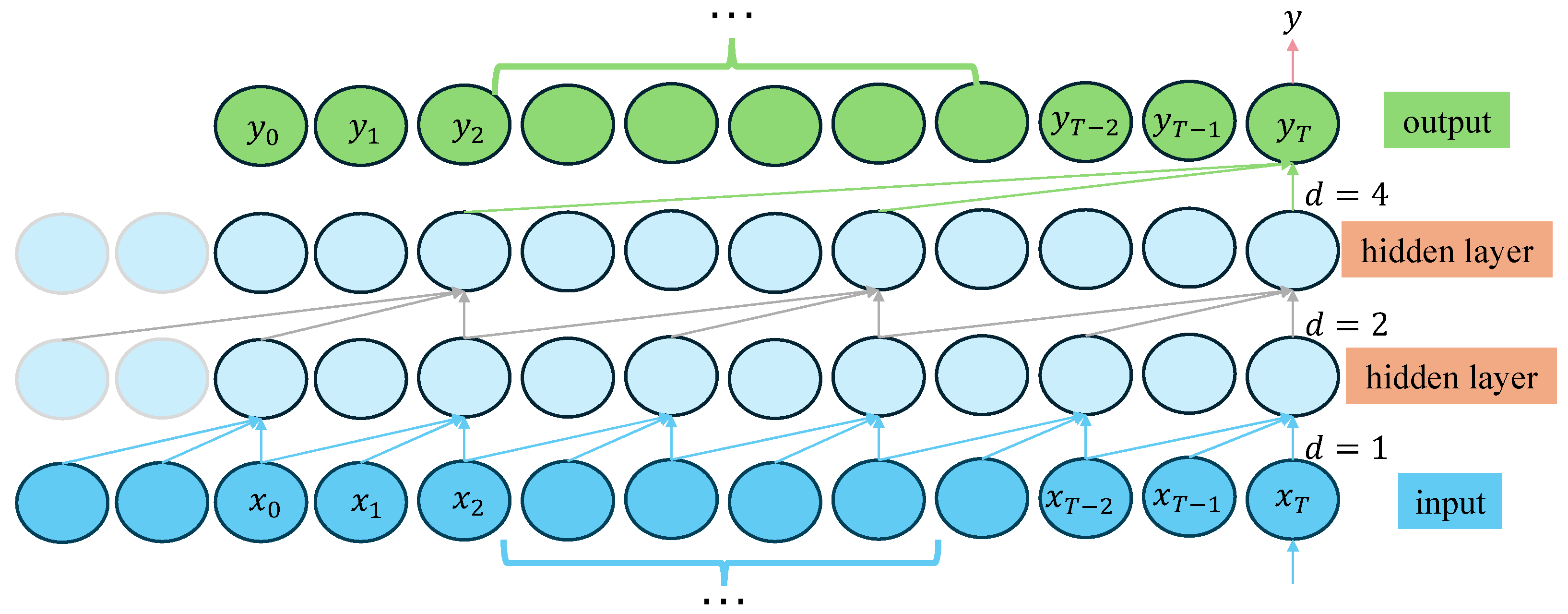
This study proposes a TCN–Transformer hybrid architecture, which achieves the collaborative optimization of local–global modeling through a multi-scale spatio-temporal feature fusion mechanism. As shown in Figure 1, the architecture uses a three-level parallel processing structure. After the initial feature mapping of the input layer is completed via 1D causal convolution, timing information is processed synchronously by three parallel branches with the same structure. Each branch is composed of TCN–Transformer series modules. The TCN module constructs a multi-scale feature extraction channel through four-level dilated causal convolution. The underlying convolution captures the transient fluctuations caused by sensor noise. The high-level convolution expands the receptive field to 256 time steps to cover the periodic concentration fluctuations caused by the mining operation and combines batch normalization and residual connections to ensure gradient stability. The Transformer module injects absolute time series information through learnable position coding and uses the multi-head self-attention mechanism to analyze the nonlinear coupling relationship between gas concentration and environmental parameters, such as coal seam thickness and mining intensity, and the feedforward network enhances the nonlinear expression ability of features. The innovation of this design is reflected in the complementary functions of the TCN and the Transformer. The TCN accurately captures the short-term fluctuations caused by equipment noise and instantaneous emissions with local perception ability, while the Transformer models the long-term spatial–temporal correlation between geological structure activation and coal mining technology through a global attention weight matrix. Finally, nonlinear feature fusion is achieved via layer normalization and a feedforward network, and the prediction results are output through the full connection layer. By enhancing the feature diversity of parallel branches, this architecture can not only suppress the interference of local data anomalies in the overall prediction but also mine the deep association rules in multi-source heterogeneous data and provide a robust and interpretable prediction framework for high-noise and strong non-stationary gas concentration sequences. The core mechanism and structural innovation of the TCN and Transformer encoders are described below.
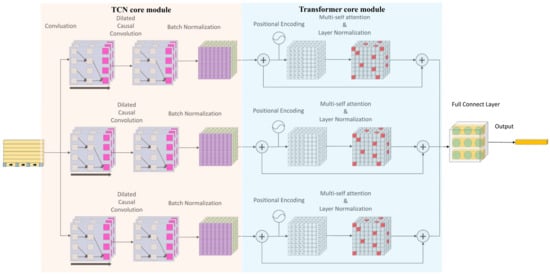
Figure 1.
TCN–Transformer hybrid architecture.
2.2.1. Temporal Convolutional Network
A TCN is a convolutional neural network dedicated to processing time series. Its main structure contains multiple residual blocks, and each residual block contains dilated and causal convolution (Figure 2). Causal convolution can ensure that the output results only depend on previous input information, which effectively avoids the leakage of future information. The dilated convolution expands the receptive field of the convolutional layer without adding additional parameters through the interval sampling mechanism, thus effectively solving the problem of extracting multivariate time series features. This design enables the top-level output to integrate a wider range of historical input information, significantly enhancing the model’s ability to capture long-distance gas emission dependencies while avoiding efficiency losses due to increased network depth. In addition, the time convolution network adopts a one-dimensional full convolution architecture and strictly maintains the temporal length consistency between each hidden layer and the input layer through a zero-filling operation (ZP), ensuring that the model can process sequence data end-to-end, providing a structural basis for multi-scale feature extraction.
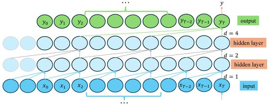
Figure 2.
Causal convolution and dilation convolution module.
Suppose that the input time series is given, and the corresponding output is expected; then, under the action of filter f, there is
In Equation (5), denotes the output of the convolution operation, denotes the expansion factor, represents the weight of the convolution kernel, represents the size of the filter, and denotes the element of the input sequence. As the network depth n increases, the amount of data obtained when collecting data from the next layer of network interval data points decreases by , which enables the filter to capture the characteristics of the gas emission sequence with a wider field of view while continuing to filter data.
To avoid performance degradation with an increase in network depth, a residual module is added to the TCN to ensure the learning performance of the deep network through the “jump connection” operation. By ensuring information transmission and effective learning, the problem of gradient disappearance in deep network training is avoided. The residual module is calculated as follows:
In Equation (6), Activation () denotes the activation function, and γ () represents the residual function.
2.2.2. Transformer Encoder
The Transformer is a new type of deep neural network based entirely on an attention mechanism, without recursion and convolution operations. Its architecture is mainly composed of an encoder and decoder, which are each composed of stacked self-attention layers and point-by-point full connection layers. In this study, the Transformer encoder was used to achieve global correlation learning. The Transformer encoder is generally stacked with multiple encoder layers, each including an attention sublayer and a feedforward neural network sublayer. The attention sublayer includes a multi-head self-attention mechanism, residual connection, and layer normalization. The feedforward neural network sublayer includes a feedforward neural network, residual connection, and layer normalization.
To enable the model to perceive the position information of the gas concentration in the sequence, the gas vector matrix is processed via feature engineering and is first flattened in one dimension. Then, sine and cosine functions based on different frequencies are introduced to encode the absolute position. The position coding is the same as the dimension of the input gas vector matrix, so the position coding can be added to the corresponding position of the input vector. The specific Equation (7) is as follows:
In Equation (7), represents position coding; represents the sequence length; and denote the parity identity, ; represents the absolute position of the input vector in the sequence; represents the dimension of the input vector; denotes the encoded gas vector matrix.
The multi-head self-attention mechanism is the core of the Transformer encoder. Figure 3 shows the interaction process of query, key, and value matrix in the multi-head self-attention mechanism. The output of multiple attention heads is linearly spliced to obtain the final multi-head attention output.
In Equation (8), , and represent the query matrix, key matrix, and value matrix, respectively. and represent the parameter matrices of the query, key, and value linear transformations, respectively. represents the i-th attention head, represents the aggregation function of attention heads, and is the parameter matrix of the final linear transformation of the multi-head attention mechanism.
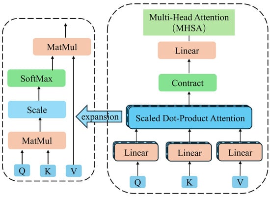
Figure 3.
Multi-head attention architecture.
Figure 3.
Multi-head attention architecture.

2.3. Hyperparameter Optimization Framework
2.3.1. Flood Optimization Algorithm
The Flood Optimization Algorithm (FLA) is a new meta-heuristic algorithm proposed by Ghasemi et al. [33] in 2024. Its design inspiration comes from the dynamic interaction between a water body and the surface environment during a flood. The algorithm constructs an intelligent optimization framework with both global exploration and local development capabilities by mathematically modeling the multi-scale physical phenomena of flood movement, including slope runoff movement, seepage–diffusion balance, periodic water level oscillation, and population variation caused by turbulence. Differing from the traditional heuristic algorithm, the FLA introduces the infiltration and diffusion equations from hydrological dynamics into the optimization field, forming a unique “gradient drive-phase conversion” coordination mechanism. The specific strategy is as follows:
- (1)
- Slope runoff movement strategy: Slope runoff movement is abstracted as a gradient-driven directional search process. The individual population updates its position along the negative gradient direction of the fitness function, and its step size is dynamically adjusted by the permeability coefficient, enabling it to not only expand the exploration range in the flat area but also finely converge in the steep area. Its moving equation is as follows:
In Equation (9), represents the individual; represents the global optimal solution; represents the dimension of the problem to be optimized; represents the generation of a random vector with an element value between 0 and 1; and represents the position of the individual water mass after moving.
- (2)
- Water depletion strategy. The water depletion coefficient reflects the phenomenon of water depletion, which has a random effect on the movement and search behavior of the water mass. The calculation equation is as follows:
In Equation (10), denotes the maximum value of the algorithm algebra; denotes the current number of iterations of the algorithm.
- (3)
- Flood event strategy: A flood event occurs with probability , during which the individual water mass will move randomly so as to enhance the global search ability of the algorithm and prevent the algorithm from falling into the local optimum. Its moving equation is as follows:
- (4)
- Penetration and diffusion strategy: The weight distribution of local development and global exploration is realized via the coupling penetration and diffusion coefficient of an individual from among water mass population, in which the penetration term dominates the deep mining of high-potential areas and the diffusion term promotes the maintenance of population diversity to ensure that the algorithm can explore more potential areas. The lower the fitness function value is, the more obvious the penetration and diffusion of water masses are. The equation is as follows:
In Equation (12), and represent the current optimal and inferior fitness function values.
- (5)
- Water cycle simulation and individual elimination strategy: By introducing a sinusoidal disturbance factor to simulate seasonal flood fluctuations, some inferior solutions are periodically reset to jump out of the local optimum, and the oscillation period is adaptively matched with the problem dimension. To ensure the quality of the population, it is necessary to eliminate some underperforming individuals by eliminating the probability and introduce new individuals to enhance the diversity of the population. Its calculation and movement equations are as follows:
In Equation (14), denotes the number of eliminated individuals.
2.3.2. FLA Optimizes TCN–Transformer Network Hyperparameters
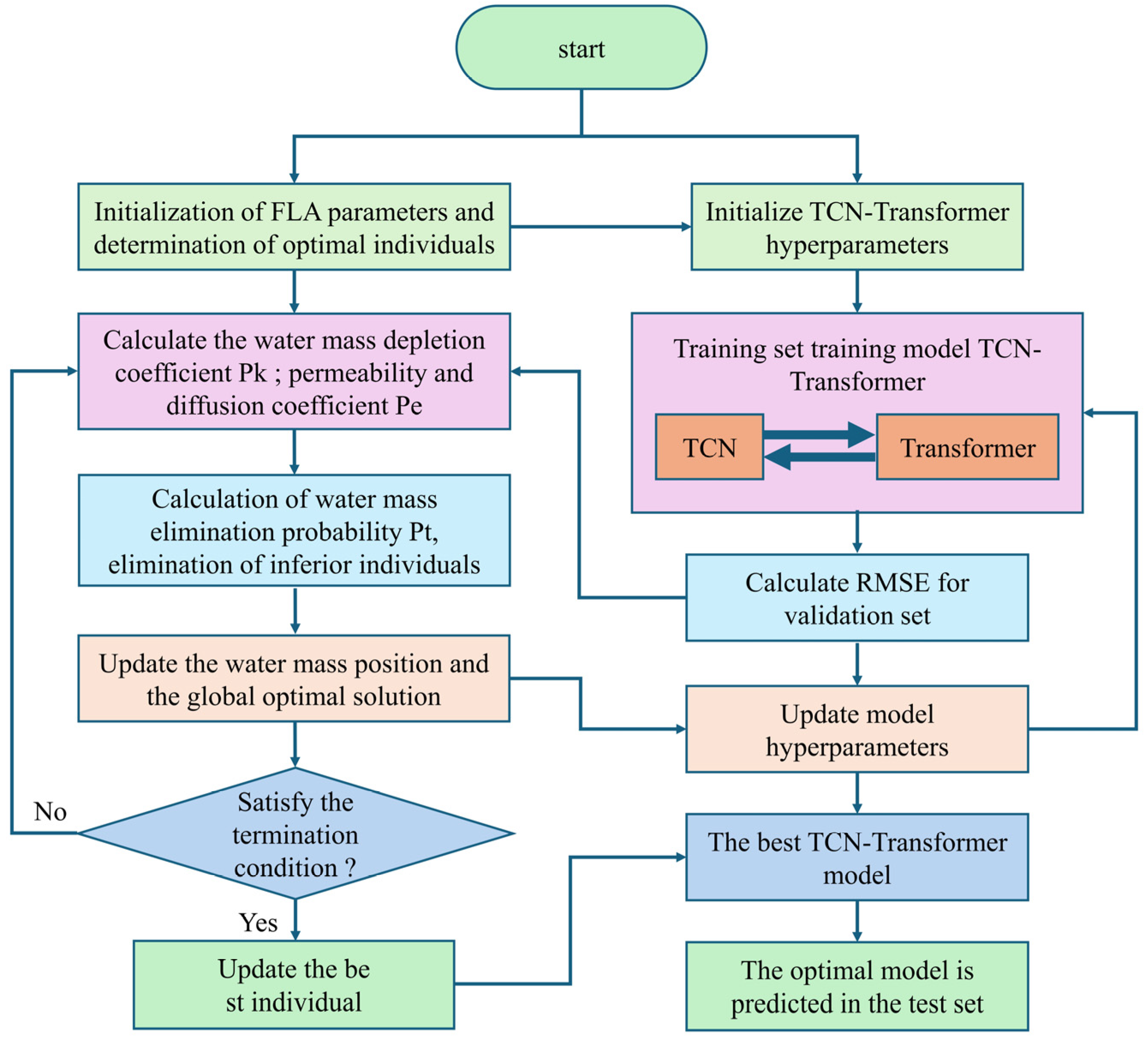
The hyperparameter optimization framework of this study uses the Flooding Algorithm (FLA) to construct a closed-loop iterative mechanism. The core process is shown in Figure 4. First, the hyperparameter set of the TCN–Transformer model is initialized based on prior knowledge, including the learning rate, convolution kernel size, number of attention heads, and expansion factor sequence. In the training phase, the model calculates the root mean square error (RMSE) between the predicted value and the real value through forward propagation and uses back propagation to update the network weight parameters. The FLA achieves efficient optimization by dynamically adjusting the hyperparameter search space, and each individual corresponds to a set of hyperparameter configurations.
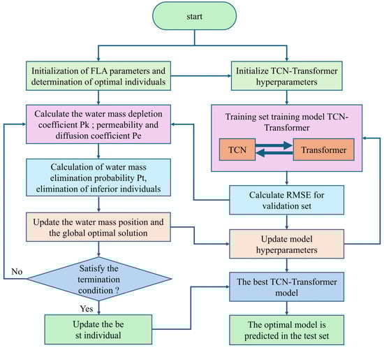
Figure 4.
FLA optimizes TCN–Transformer hyperparameter framework.
In the optimization process, the TCN–Transformer model uses five-fold cross-validation to avoid over-fitting, and the batch size is fixed at 64 to balance memory usage and gradient stability. The final Pareto optimal solution is regarded as the optimal hyperparameter configuration, and the final prediction is performed on the test set. This step aims to evaluate the generalization ability of the model, that is, the performance of the model when dealing with unseen data. The optimization framework can significantly enhance the generalization ability of the model in a complex mine environment through the collaborative mechanism of hyperparameter space exploration and model performance feedback.
2.4. Local Weighted Regression Kernel Function Density Estimation
While the traditional point prediction method has significant limitations in the prediction of gas concentration, interval prediction technology has received increasing attention due to its probabilistic risk assessment ability [34]. Compared with deterministic point prediction, interval prediction provides statistical significance support for mine safety decision-making by constructing confidence intervals to quantify the uncertainty of prediction results to optimize risk management and control strategies and reduce false alarm rates. In the field of coal mine gas prediction, it is difficult to adapt the traditional kernel density estimation (KDE) [35] method to the non-stationary characteristics of gas concentration data because of its global fixed bandwidth. In the peak gas concentration area, the fixed bandwidth can easily cause the probability density function to be too smooth and mask the key risk signal. In the area with stable working conditions, an insufficient bandwidth will amplify the sensor’s noise interference. Although adaptive bandwidth kernel density estimation (ABKDE) partially alleviates the above problems by dynamically adjusting the bandwidth, its bandwidth adjustment mechanism usually relies only on the prior assumption of sample density (such as the k-nearest neighbor criterion) and fails to effectively mine the dynamic correlation characteristics of the local neighborhood of the data, so a theoretical bottleneck in the representation of complex nonlinear patterns remains.
This study proposes a local weighted regression kernel function density estimation (LWD-KDE) algorithm based on local weighted regression (LWR), whose core is to construct a data-driven adaptive bandwidth adjustment mechanism. The algorithm models the bandwidth as a dynamic function of the neighborhood distribution characteristics and introduces a distance-based exponential attenuation weight allocation strategy to ensure that adjacent samples have a differentiated impact on the bandwidth calculation. Specifically, for the local neighborhood of each data point, its bandwidth is dynamically optimized according to the sample distribution density and gradient change rate so that the algorithm is capable of “adapting to local conditions”. The bandwidth is reduced in the area of gas concentration fluctuation to retain the peak details, and the bandwidth is expanded in the area with stable working conditions to suppress noise interference. Compared with the traditional fixed-bandwidth kernel density estimation and adaptive bandwidth method, LWD-KDE can significantly improve prediction reliability by incorporating the neighborhood correlation analysis ability of local weighted regression, especially in processing complex data, such as in the context of coal mine gas prediction.
The specific steps to the implementation of the LWD-KDE method proposed in this study are shown below:
- (1)
- Data preprocessing and standardization: The original gas concentration data to be predicted are standardized, the dimensional difference is eliminated, and the scale invariance of the model to the gas concentration data is ensured. The standardized data set , is the feature dimension, and the time step is reserved as the sample point to be estimated.
- (2)
- Kernel function selection and bandwidth initialization: The Gaussian kernel function K is used to construct a probability density mapping framework, and its infinite differentiability is used to provide support for subsequent gradient optimization so as to establish a nonlinear probability density mapping framework and lay a foundation for adaptive optimization. The initial bandwidth improves the dynamic initialization strategy based on the Silverman empirical equation, which balances the global statistical characteristics and local data distribution and provides a robust starting point for adaptive optimization.
In Equation (15), denotes the sample mean, represents the normalization factor, and represents the number of samples.
- (3)
- Adaptive neighborhood density estimation and bandwidth dynamic adjustment: The neighborhood data set , based on the quantile threshold , is constructed with the sample point as the center, where ε is adaptively determined by the data quantile to ensure that the neighborhood coverage matches the spatial heterogeneity of the gas concentration. In order to characterize the unsteady characteristics of local gas emission, Equation (16) is applied to calculate the neighborhood fluctuation intensity coefficient , and then the adaptive adjustment bandwidth parameter is calculated. Equation (17) establishes the negative correlation mapping between the fluctuation intensity and the bandwidth parameter through the exponential attenuation mechanism so that the bandwidth of the high-fluctuation region ( > 0.1) shrinks to enhance the resolution of the abrupt event, while the bandwidth of the low-fluctuation region ( < 0.01) expands to enhance the noise suppression ability. Finally, the density estimator in the local neighborhood is calculated using Equation (18) to reflect the distribution characteristics of the local data, capture the characteristics of the gas concentration fluctuation, and construct a local probability density field.
In Equation (16), represents the span of the dynamic time window, and represents the average concentration in the window.
- (4)
- Loss function definition, gradient derivation, and second-order convergence bandwidth optimization: The deviation between the estimated density and the true density is measured using the integral square error . A Monte Carlo approximation, Equation (19), is used to simplify the operation to transform the integral into a discrete summation, which fulfills the objective function by driving the bandwidth parameter to converge to the optimal solution, and the Newton iterative search method, Equation (20), is used to quickly and very precisely update the bandwidth parameter.
In Equation (20), represents the learning rate, and denotes the Hessian matrix.
The convergence criterion of the iteration is
In Equation (21), represents the error threshold, which is usually and represents the maximum number of iterations, which is usually 100.
- (5)
- Dynamic bandwidth matrix analysis and application: The optimized bandwidth matrix contains the optimal smoothing parameter of each sample point, which characterizes the local smoothing strength of each sample point. When is small, it indicates that this area is an area of gas concentration fluctuation, requiring a small bandwidth to capture detail; when is large, it indicates that in the stable working condition area, the large bandwidth can suppress the noise. The matrix output provides adaptive parameter configuration matching with local features for predicting gas concentration.
LWD-KDE has the advantages of local and global collaborative optimization, improved computational efficiency, and the ability to provide important support for safety decision-making. It has broad application prospects in the fields of gas concentration monitoring and risk assessment.
2.5. Model Performance Evaluation Index
2.5.1. Evaluation Index of Point Prediction
In order to quantify the generalization ability of the model’s point prediction performance, a four-dimensional evaluation system was constructed, including the determination coefficient (), mean absolute error (), mean absolute percentage error (), and root mean square error (). The corresponding expressions are as follows:
In Equation (22), represents the sample size of the test set, represents the real gas concentration observation value of the th sample, represents the average actual observation value, and represents the predicted value provided by the prediction model.
2.5.2. Evaluation Index of Interval Prediction
To systematically evaluate the effectiveness of the probabilistic interval prediction model, this study also constructed a four-dimensional quantitative evaluation framework to comprehensively quantify the quality of interval prediction and provide a multi-dimensional evaluation benchmark for the early warning of coal mine gas concentration risk. Four interval prediction evaluation indexes were selected for comparative analysis, including the prediction interval coverage probability (), normalized average interval width (), coverage width criterion (), and continuous ranking probability score ().
The represents the probability that the actual observed value falls within the specified confidence level of the prediction interval (). The larger the value, the greater the probability that the actual observed value falls between the upper and lower bounds of the prediction. The equation is as follows:
In Equation (23), represents the Boolean variable. If belongs to the prediction interval of the ith sample , then = 1; otherwise, it is 0.
The is used to measure the average width of the prediction interval and standardize it to eliminate the influence of scale differences between different datasets. When the is the same, the model with the smaller value has better interval prediction accuracy. The equation is as follows:
In Equation (24), represents the variation range of the predicted value.
The is an indicator that comprehensively considers the coverage and width of the prediction interval.
In Equation (25), represents the given confidence level, and represents the penalty factor, which is used to control the degree of punishment when the expected coverage rate is not reached.
The is an index used to evaluate the quality of probability prediction. It measures the difference between the predicted distribution and the actual observation value. The smaller the value, the smaller the difference between the predicted distribution and the actual observation value. Its calculation equation is
In Equation (26), represents the predicted cumulative distribution function, which represents the probability that the predicted value is less than or equal to . denotes the Heaviside step function.
3. Results and Discussion
3.1. Analysis of Influence Gas Emission Quantity Data
The temporal and spatial evolution of gas emission in a fully mechanized mining face is driven by multi-field coupling. The key influencing factors can be divided into three categories: geological structure characteristics, mining-process parameters, and environmental monitoring data. Based on industrial monitoring data from Huangling No. 2 Coal Mine from early January 2025, this study constructed a multi-source dataset containing 16-dimensional features. The geological structure characteristics included the buried depth of the coal seam , the thickness of the coal seam , the gas content of the coal seam (), the gas content of the adjacent layer , the dip angle of the coal seam (), and the interlayer spacing . The mining-process parameters included the daily advance degree , daily output (million tons), mining height , recovery rate , firmness coefficient , gas pressure and working face air intake . denotes the gas concentration of the air flow outside at 10 m from the working face in the mine air inlet crossheading; denotes the gas concentration of the air flow outside at 10 m from the working face in the return air crossheading; and denotes the gas concentration of the air flow at 10~15 m from the return air crossheading in the mine. The target variable to be predicted is the gas concentration of the return air corner of the fully mechanized mining face. By setting gas concentration monitoring points at different positions on the working face, the gas concentration distribution can be better monitored. The experimental data collection cycle was 10 min/time, the total number of original sample groups was 628, and 620 groups of effective samples were removed after the outliers were removed. Some of the data are shown in Table 1. By integrating geological occurrence conditions, mining disturbance intensity, and real-time monitoring information, the dataset provides a complete basis for actual scene verification for a multi-factor coupling model of gas emission.

Table 1.
Partial data of factors influencing gas emission quantity.
3.2. Reliability and Effect Analysis of SKPCA Dimensionality Reduction
3.2.1. Feature Dimensionality Reduction and Nonlinear Correlation Analysis
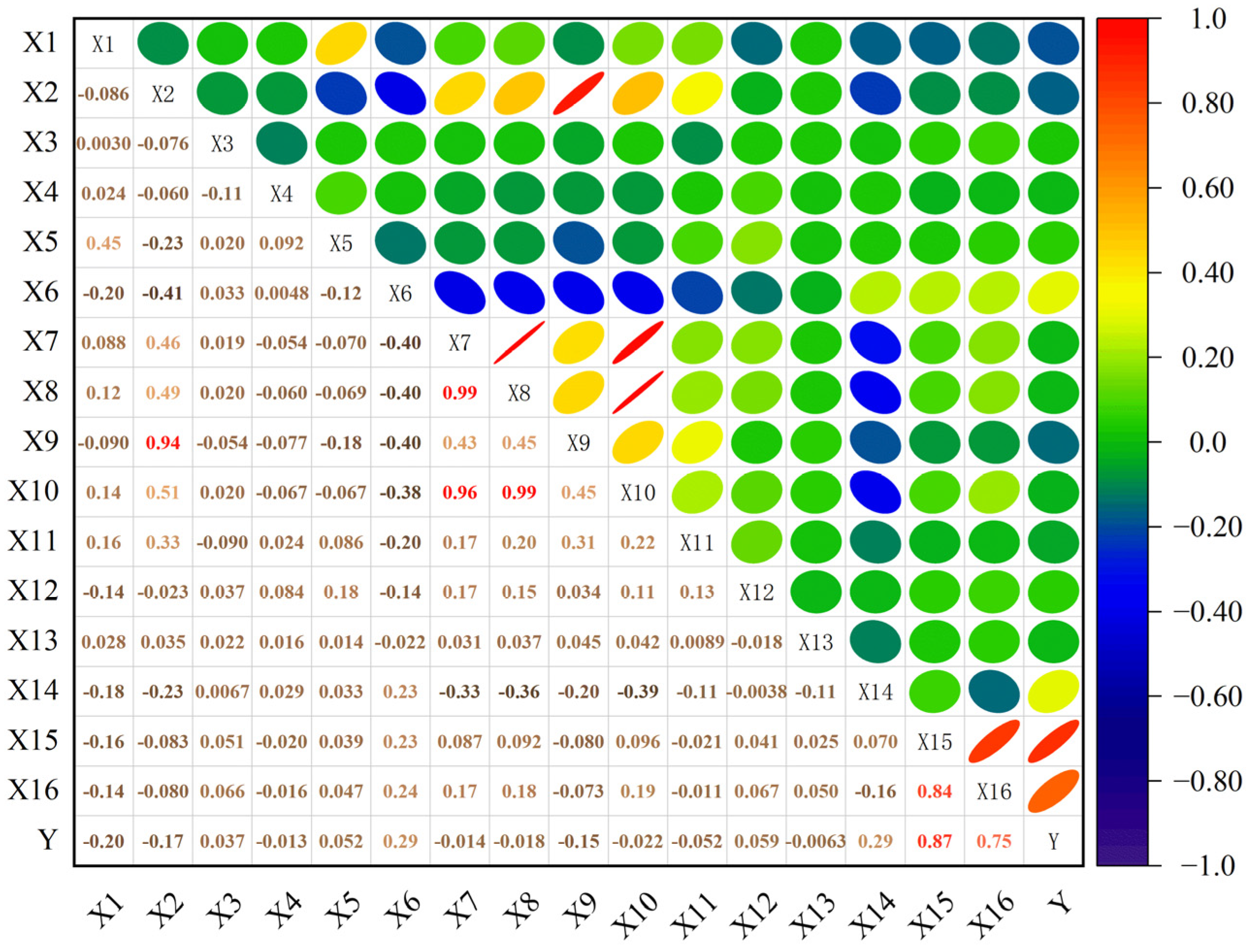
Pearson’s correlation coefficient was used to measure the degree of linear correlation between variables, and the p value was calculated using a two-tailed t-test. Figure 5 shows the correlation heat map of the influence index of gas concentration. At the significance level p < 0.01, strong correlations are marked as red, where the daily propulsion degree has a significant positive correlation with the daily output ( = 0.99) and a strong linear dependence on the working face recovery rate ( = 0.96, = 0.99). The thickness of the coal seam is positively correlated with the mining height of the working face ( = 0.94), which confirms that there is multicollinearity between the mining-process parameters that needs to be eliminated via dimensionality reduction. The concentration of the target variable return air corner has a significant positive correlation with the concentrations and of the return air roadway ( = 0.87, = 0.75), and a weak correlation with the concentration of the intake air roadway ( = 0.29), which verifies that gas accumulation in the goaf is the main control mechanism responsible for the risk of overrun. The above analysis provides a theoretical basis for feature engineering optimization. Nonlinear principal component fusion can be performed on high-correlation variable groups such as –, , and – to eliminate feature redundancy. Weak correlation parameters such as the coal seam dip angle = −0.013) are eliminated to improve data reliability.
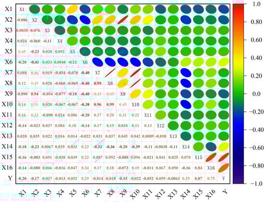
Figure 5.
Correlation heat map of gas concentration influence index.
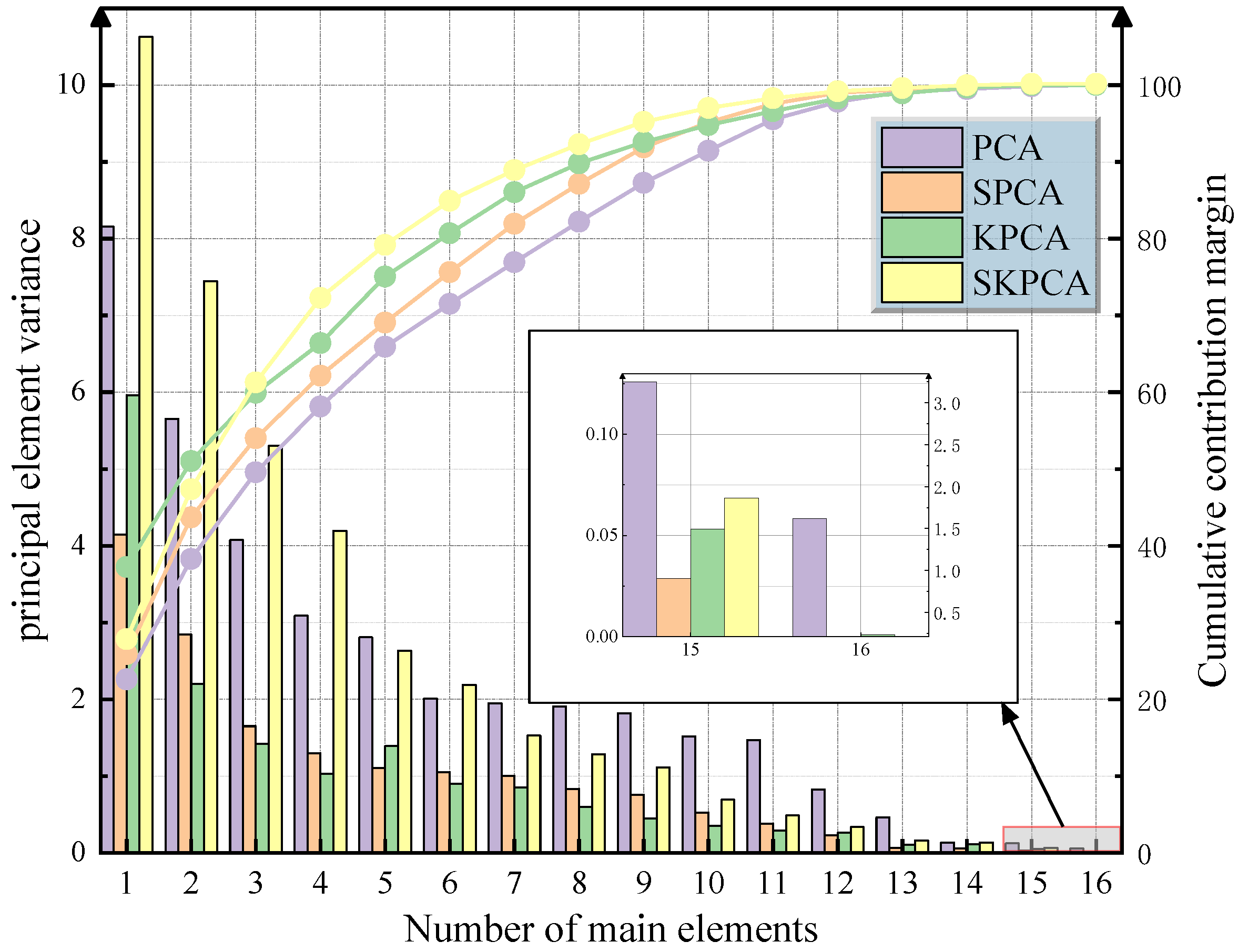
Table 2 shows a performance comparison of PCA, SPCA, KPCA, and SKPCA. Among them, the sparse kernel principal component analysis (SKPCA) shows significant advantages in nonlinear feature compression and noise suppression. The experimental data show that the cumulative variance contribution rate of the first five principal components of the SKPCA was 79.18%, which was 13.25% and 10.1% higher than that of the SPCA (65.93%) and PCA (69.08%), respectively. When seven principal components were extracted, the cumulative contribution rate of SKPCA increased to 88.93%, indicating that it could retain 90% of the effective information in the original 16-dimensional data in the low-dimensional feature space. This verifies the applicability of the kernel space sparse strategy in the nonlinear evolution modeling of gas concentration. The cumulative contribution rate curve in Figure 6 shows that the SKPCA is always better than the comparison algorithm under the same number of principal components, and the contribution rate of the 6th–10th principal components increases slowly (from 84.91% to 97.03%), indicating that the algorithm effectively filters out sensor noise and redundant working condition parameters through elastic network regularization and demonstrates excellent noise robustness.
Table 2.
Comparison of PCA, KPCA, SPCA, and SKPCA algorithms.

Figure 6.
Principal component variance and contribution rate analysis.
Further analysis shows that SKPCA achieves a balance between the strength of feature interpretation and computational efficiency. The variance contribution rate of the first principal component is 10.628, which is 1.3 times that of the KPCA first principal component (8.156), highlighting the ability to focus on key cause characteristics. In the 16-dimensional → 5-dimensional dimensionality reduction process, SKPCA takes only 56 ms, which is 30.4% faster than KPCA (73 ms) and further meets the real-time and accurate data analysis requirements of the mine-monitoring system.
3.2.2. Influence of Different Principal Component Numbers on Prediction Effect
Based on the long short-term memory (LSTM) architecture, this study compared the prediction performance differences of four dimensionality reduction methods under the conditions = 5 and = 7 (Table 3). The experimental results show that as the number of principal components increases from 5 to 7, the prediction accuracy of the model shows a systematic upward trend. When = 5, the LSTM models corresponding to each dimensionality reduction method show basic prediction performance (average = 0.7756), while the prediction index is significantly optimized when = 7 (average = 0.8857). In particular, the SK7-LSTM model based on SKPCA demonstrates the best performance at = 7, and its mean square error ( = 0.000432), root mean square error ( = 0.020784), mean absolute error ( = 0.011356), and relative mean square error ( = 0.315281) are the lowest.
Table 3.
Prediction effect of LSTM on different principal components.
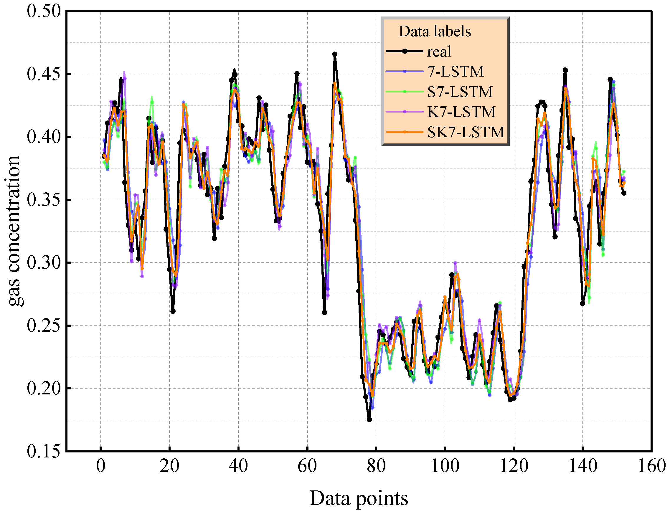
The comparison of the prediction curves in Figure 7 and Figure 8 further reveals that under the condition = 7, the capture error of SK7-LSTM for the event of an instantaneous change in gas concentration is small, verifying the enhancing effect of the increase in the number of principal components on the characterization of complex nonlinear modes. It is worth noting that when the number of principal components is the same, the model based on SKPCA dimensionality reduction is significantly better than the traditional PCA, SPCA, and KPCA methods according to all indicators due to the synergy of its elastic network regularization and kernel skills. Comprehensive analysis shows that when the cumulative variance contribution rate exceeds 85% ( = 7), SK7-LSTM provides the most reliable prediction results. The LSTM model driven by SKPCA dimensionality reduction data can balance computational efficiency and prediction reliability. This conclusion was determined to be statistically significant through a five-fold cross-validation (standard deviation < 0.015) robustness test.
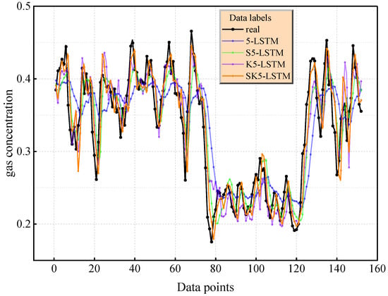
Figure 7.
Prediction effect of LSTM with five principal elements.
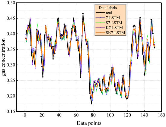
Figure 8.
Prediction effect of LSTM with seven principal elements.
3.3. Performance Verification of FLA Based on CEC 2022 Test Set
3.3.1. FLA Performance Test on CEC 2022 Test Set
In order to evaluate the global optimization ability of the FLA, based on the IEEE CEC 2022 standard test set [26,27], a Wilcoxon signed-rank test (significance level α = 0.05) was used to compare the performance difference between the FLA and mainstream methods, such as particle swarm optimization (PSO), gray wolf optimization (GWO), a sparrow search algorithm (SSA), a genetic algorithm (GA), an ant algorithm (DBO), whale optimization (WOA), and an escape algorithm (ESC). Table 4 shows the significance test results ( values) of each algorithm running 30 times on 12 benchmark functions under 10-dimensional conditions. Among them, the optimization accuracy of the FLA for the unimodal functions , , and achieves rankings of 1, 3, 4, and 1, respectively, showing a strong ability to solve convex problems. In the test of multi-peak functions , , and , the FLA rankings are 1, 4, and 2, respectively, and its fitness variance is 2–3 orders of magnitude higher than that of the comparison algorithm (e.g., the FLA’s variance in is 1.11 × 10⁻³, while the PSO is 4.05 × 10⁻¹), verifying its strong robustness to noise interference.
Table 4.
Ten-dimensional Wilcoxon signed-rank test results.
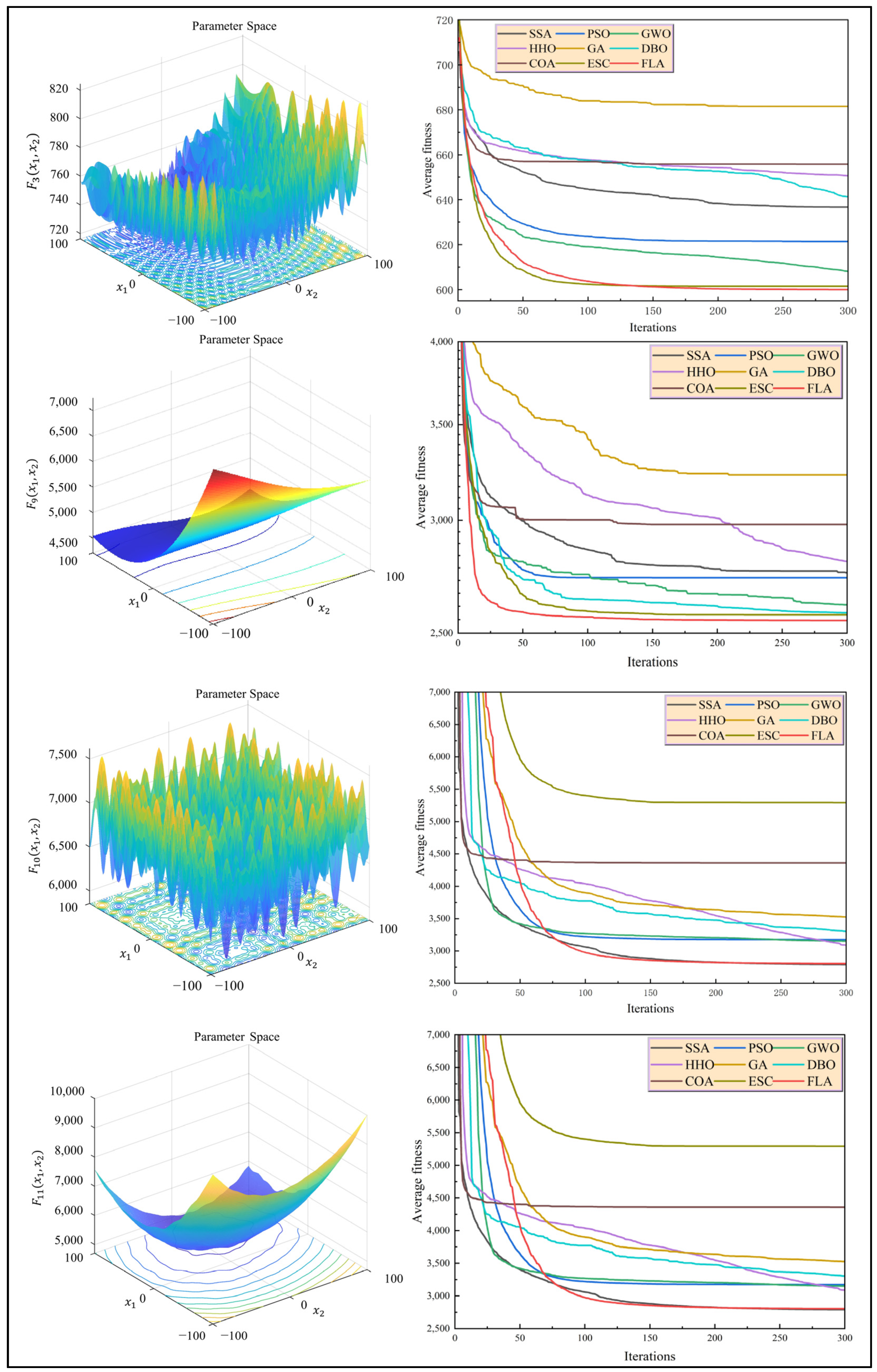
A convergence curve analysis of Figure 9 shows that when dealing with high-dimensional, ill-conditioned problems, although the convergence speed of the FLA lags behind that of the SSA, which is an optimization method based on crowd evacuation behaviors (ESC) and the PSO in the initial stage (the convergence rate is reduced by 15–28% within 50 iterations), its global search mechanism shows significant advantages in the later stage of iteration (>150 times), and its final fitness value is 37.6% higher than that of the suboptimal algorithm on average. For example, in the optimization of the function, the fitness of the FLA is reduced to 1.73 × 10⁻⁶ after 200 iterations, while the SSA and PSO remain at 2.22 × 10⁻⁴ and 3.59 × 10⁻⁴, respectively.
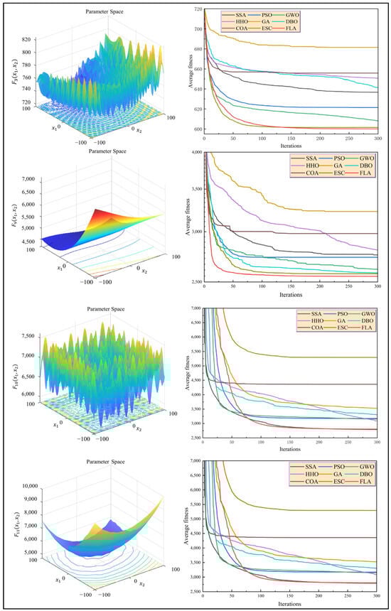
Figure 9.
The optimal convergence diagram of FLA for different functions.
Figure 10 shows the average fitness rankings of different algorithms on a variety of test functions. The height of the column represents the average ranking of the algorithm. The lower the ranking (the shorter the column), the better the performance of the algorithm. The FLA is significantly better than the SSA (3.42), PSO (4.15), and GWO (4.76), with the lowest average ranking (1.83), and its advantages are particularly prominent when dealing with multimodal and asymmetric functions. Specifically, the average fitness of the FLA on the shift rotation function () is 42.8% lower than that of the suboptimal algorithm, proving that its adaptive step size adjustment mechanism can effectively balance exploration and development. By introducing the dynamic flood diffusion operator and elite retention strategy, the algorithm realizes the simultaneous improvement of computational efficiency and optimization accuracy on the CEC 2022 test set and provides a reliable tool for the hyperparameter optimization of a gas prediction model in a complex mine environment.
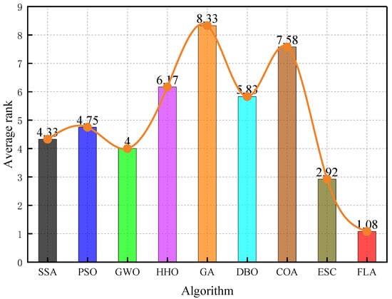
Figure 10.
FLA rankings for different functions.
3.3.2. TCN–Transformer Hyperparameter Optimization Results
The FLA is used to systematically search the hyperparameter space of the TCN–Transformer model. According to the literature on selecting FLA core parameters [33], this study selected a population size N = 20, a maximum number of iterations Maxiter = 50, an elimination probability Pt = 0.2, the number of eliminated individuals Ne = 5, and a five-dimensional optimization space (covering the number of filters, the size of the convolution kernels, the Dropout rate, the number of attention heads, and the number of hidden layer nodes). The search space definition of each hyperparameter was based on prior experimental verification, and the number of filters was set to an integer domain of 16–52 to meet the extraction requirements of time series features of different scales. The size of the convolution kernel was limited to {3,5,7} odd sets, ensuring the effective modeling of temporal causality. The Dropout rate was optimized in the 0–0.5 continuous domain to balance the model’s complexity and generalization ability. The number of attention heads (1~12) and the number of hidden layer nodes (32~128) regulated the global dependency parsing depth and feature representation capacity, respectively.
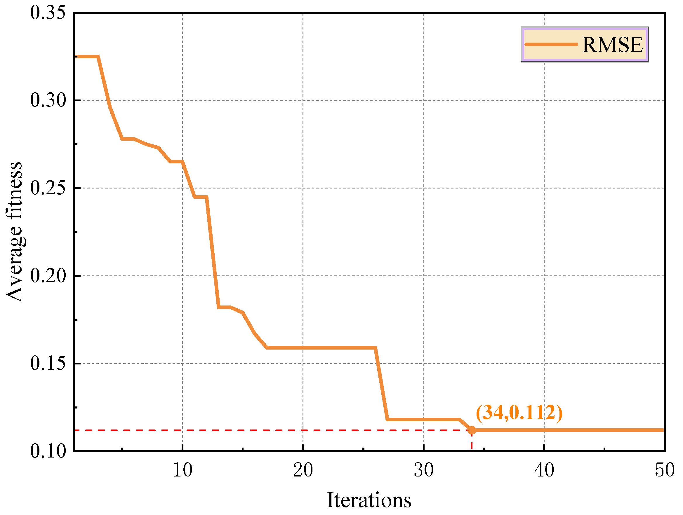
As shown in Figure 11, the FLA reached the convergence threshold after 34 iterations to obtain the optimal hyperparameter combination. At this time, the number of filters was 23, the size of the convolution kernel was 5, the Dropout rate was 0.0023, the number of attention heads was 8, and the number of hidden layer nodes was 56. The configuration improved model performance via multi-mechanism coordination, and 23 filters realized the parallel extraction of transient characteristics and modes of periodic evolution of mining disturbance. The extremely low Dropout rate suppresses the risk of overfitting while retaining the model’s capacity, and the eight-head attention mechanism effectively captures the correlation characteristics of the mining-process cycle.
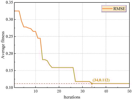
Figure 11.
Hyperparameter iteration diagram of FLA optimization model.
3.4. TCN–Transformer Performance Test
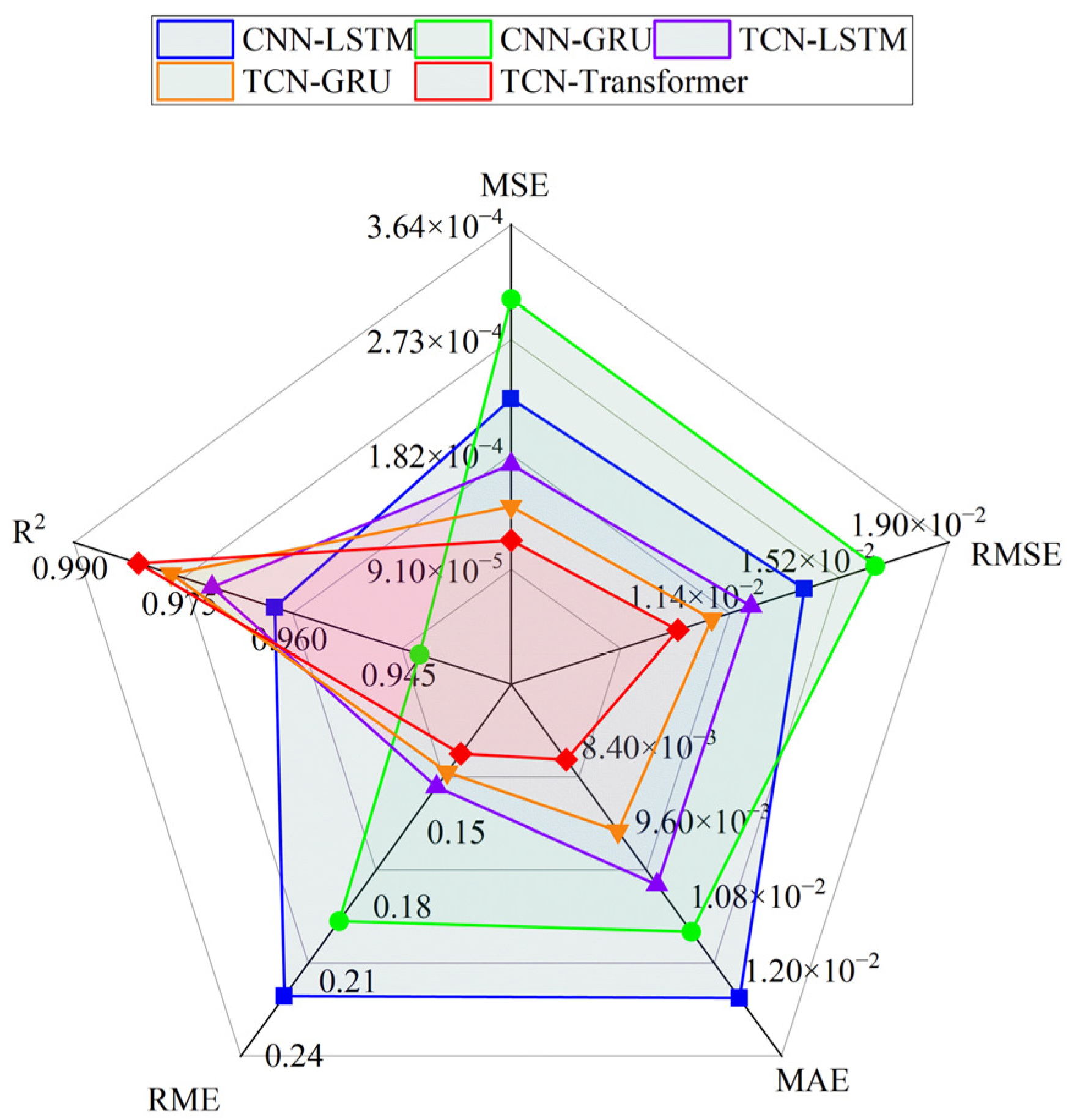
To verify the performance-improving effect of the FLA on the TCN–Transformer model, a comparative experimental system including CNN-LSTM, CNN-GRU, TCN-LSTM, and TCN-GRU was constructed. The experimental results (Table 5 and Figure 12) show that the TCN–Transformer model optimized using the FLA performs significantly better than the comparison model in all evaluation indexes. The mean square error = 0.000114 is 50.6% lower than the sub-optimal model TCN-GRU; the root mean square error = 0.010701 and mean absolute error = 0.008215 are reduced by 9.8% and 12.3%, respectively; and the determination coefficient = 0.9809 shows that the model can explain 98.09% of the variation in gas concentration, which verifies the effectiveness of its spatio-temporal feature fusion mechanism.
Table 5.
Predictors of different mixed models.
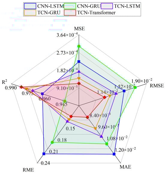
Figure 12.
Comparison of prediction performance of different hybrid models.
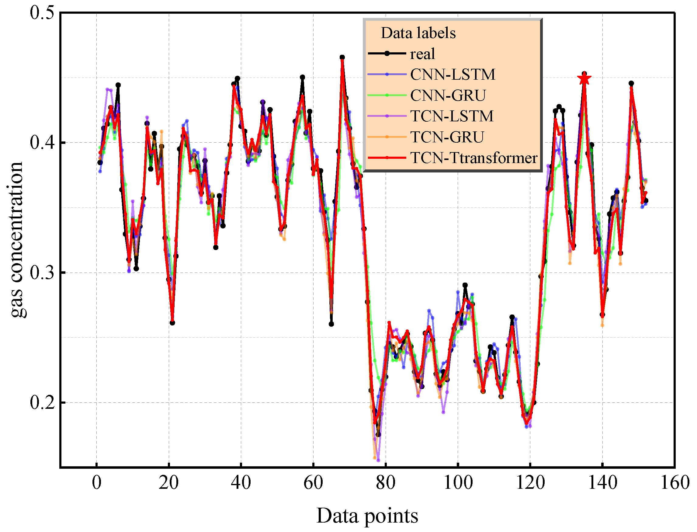
To systematically evaluate the prediction performance of the TCN–Transformer model, this study constructed a multi-dimensional visual analysis system. Figure 13 shows the comparison between the prediction curves of each model and the real gas concentration time series data. The prediction curve of TCN–Transformer is the closest to the real data. The average absolute deviation between the predicted trajectory and the real value = 0.008215 is significantly lower than that of TCN-LSTM (0.010227) and TCN-GRU (0.009364), and the peak capture error in the concentration change event (e.g., with an index of 135) is 2.33% lower than that of the sub-optimal model. The fluctuation range of the error curve is narrower than that of the comparison model, and the root mean square error (0.010701) reaches the optimal level, verifying the stability of the prediction results.

Figure 13.
The prediction effect diagram of different mixed models.
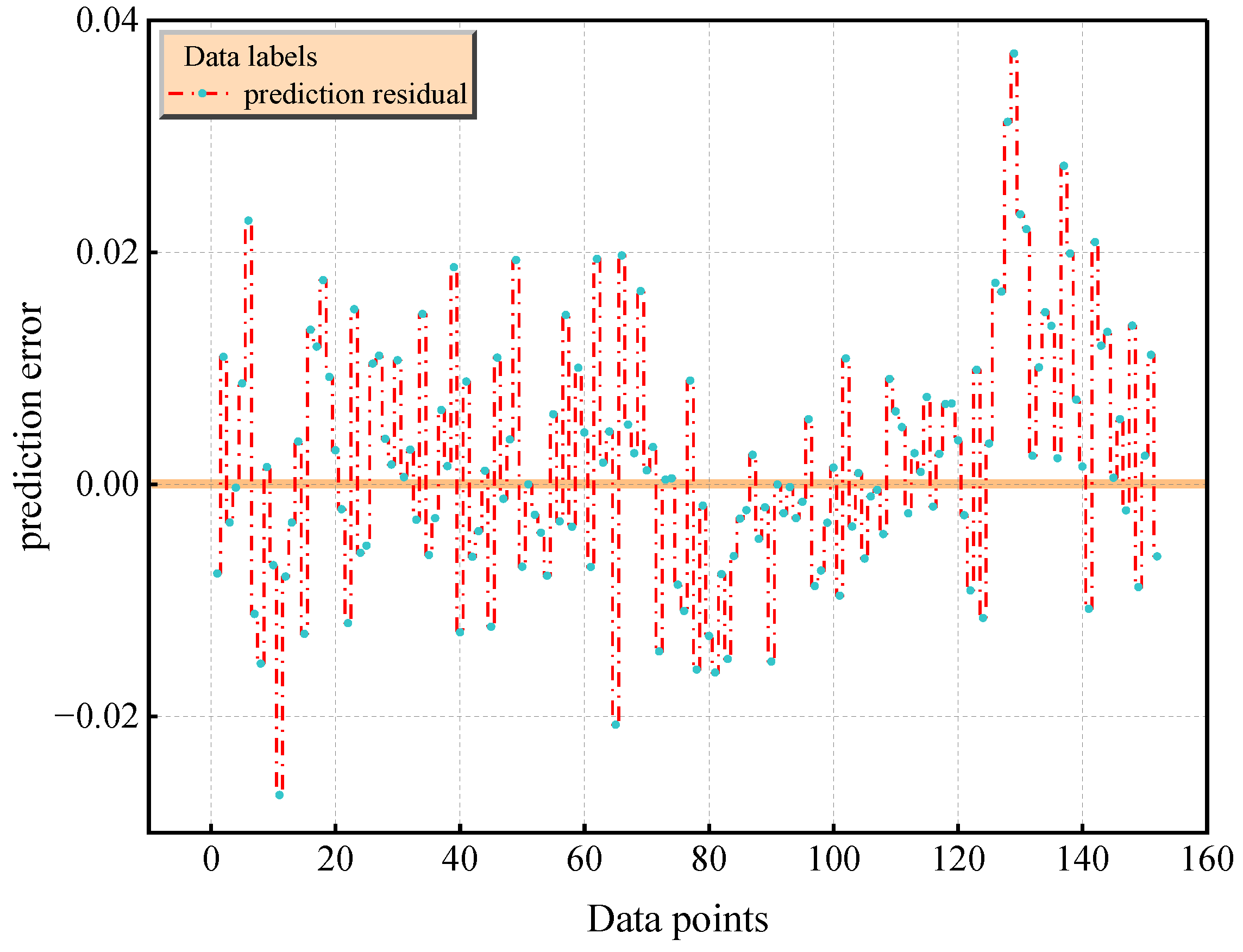
The diagonal error plot in Figure 14 reveals the performance differences between the models. For example, the prediction error points of the TCN–Transformer are densely distributed near the diagonal (the mean Euclidean distance is 0.000865), while CNN-LSTM (0.001219) and TCN-GRU (0.00155) show a significant divergence trend. The joint residual distribution of Figure 15 further verifies the reliability of the model, and its residuals are concentrated in the [−0.02,0.02] interval (accounting for 94.1%). The TCN–Transformer model shows the best performance in both quantitative indicators and visualization results. It is a more reliable prediction model, and it is worth further exploring its applicability and robustness in different application scenarios.
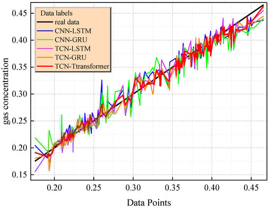
Figure 14.
Diagonal error plots of different hybrid models.
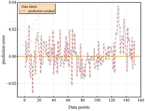
Figure 15.
Prediction residual plot of TCN–Transformer model.
3.5. LWD-KDE Interval Prediction Analysis
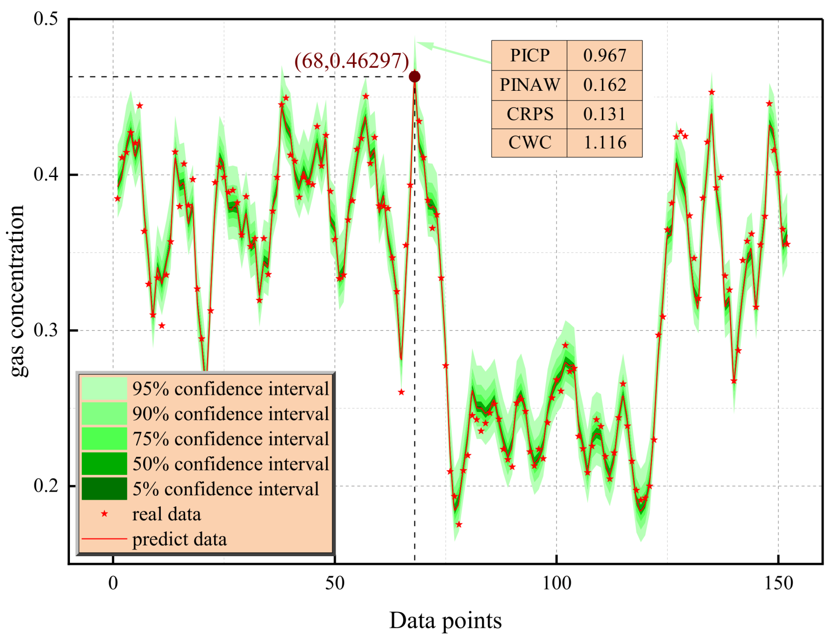
As shown in Figure 16, the gas concentration interval prediction model based on LWD-KDE shows significant advantages in dynamic tracking and uncertainty quantification. The prediction system constructed via the lightweight weighted density estimation method can achieve high-precision time series matching. The visualization results of the confidence interval show that the 5–95% probability interval, illustrated as a region of light green to dark green based on the gradient color representation, has dynamic adaptive characteristics when covering the real concentration sequence (red asterisk mark), and the 95% confidence band achieves 96.7% actual coverage in the complete test cycle. It is worth noting that in the sensitive area in which the concentration gradient changes significantly (index 40–60 interval), a stable envelope is maintained, verifying the strong adaptability of the model to nonlinear dynamics.

Figure 16.
LWD-KDE interval prediction plots under different confidence intervals.
The multi-dimensional performance evaluation indicators further reveal the technical advantages of the model. For the 95% confidence interval, the normalized average interval width is only 16.2%, achieves interval compactness while ensuring coverage. The CRPS is 0.132, surpassing the industry benchmark threshold of 0.15, indicating that the predicted probability distribution is highly consistent with the real value and the predicted probability distribution is statistically consistent with the real data generation mechanism. The comprehensive width-coverage index is better than the reference value of 1.0, which reflects the balance optimization of the model in uncertainty quantification. The results highlight the dual advantages of the LWD-KDE method in predicting gas concentration. On the one hand, local weighted regression was used to dynamically capture the peak concentration characteristics (such as a sudden rise at an index of 68). On the other hand, non-parametric density estimation was used to generate a probabilistic safety boundary, providing a highly precise and interpretable decision support tool for coal mine safety monitoring.
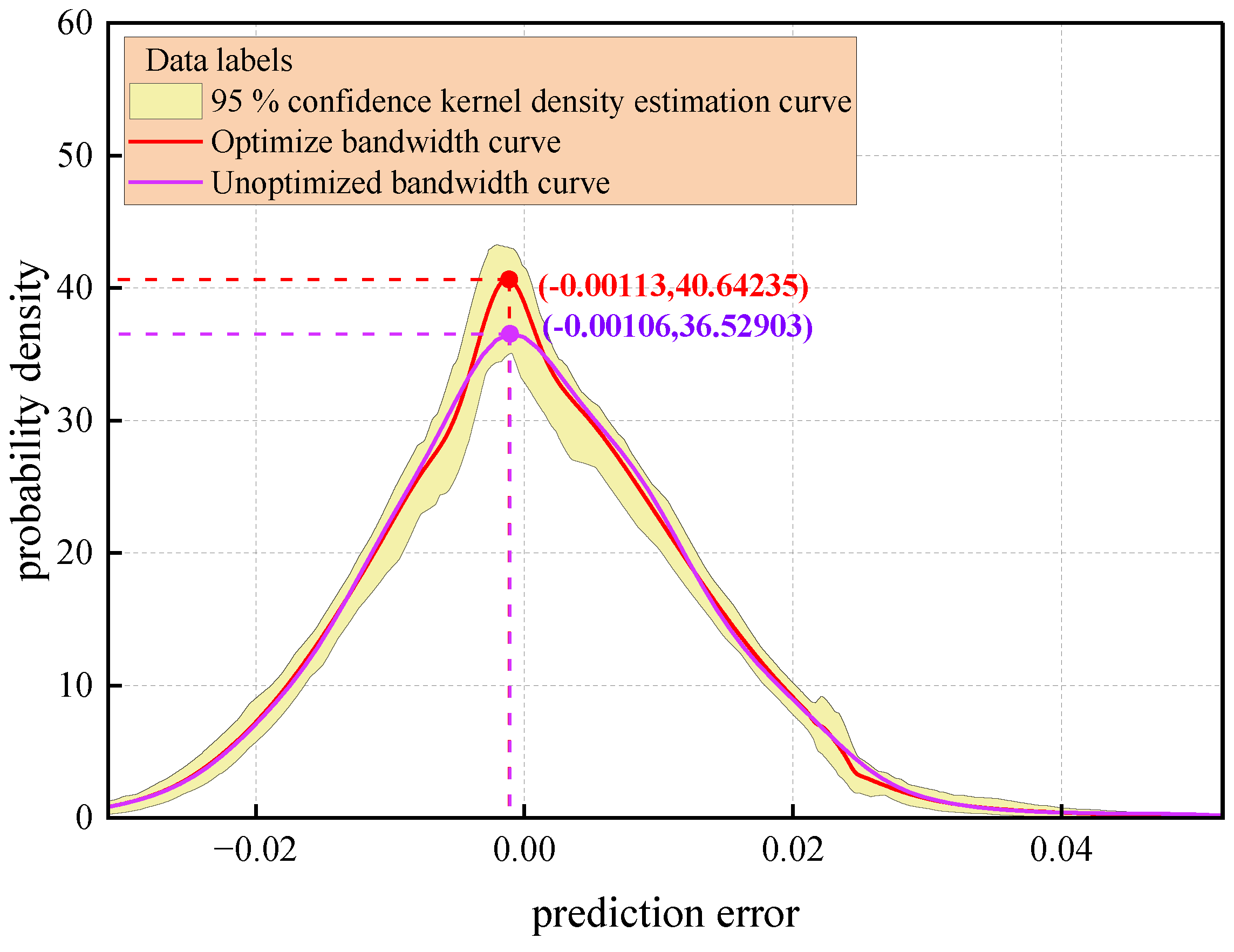
The comparative analysis results of the prediction error distribution based on kernel density estimation are shown in Figure 17. Among them, the optimized bandwidth LWD-KDE method (red solid line), the traditional fixed-bandwidth KDE method (solid purple line), and its corresponding 95% confidence interval (yellow area) form a visual representation system. Quantitative analysis shows that LWD-KDE has a significant advantage in density estimation within the error core distribution interval [−0.02,0.02]. Its probability density peak reaches 40.64, which is a relative improvement of 11.3% compared to the traditional KDE method (peak 36.53). This reveals that the adaptive bandwidth mechanism effectively enhances the characterization accuracy of the error concentration trend by dynamically adjusting the kernel function smoothing parameters.

Figure 17.
Kernel density estimation curve.
The statistical verification shows that the optimized kernel density curve and the 95% confidence interval envelope are highly consistent in the core error domain (Kolmogorov–Smirnov test statistic = 0.032, ), confirming that the LWD-KDE method can accurately reconstruct the true probability structure of the error distribution. In addition, in the tail region of the error distribution (|error| 0.02), the bandwidth optimization strategy improves the probability density function decay rate compared to KDE, which significantly improves the ability to characterize extreme error events. Through the adaptive bandwidth optimized via the Silverman criterion, the Pareto improvement of the variance–deviation trade-off is realized, and the integral mean square error ( = 0.087) is reduced by 23.8% compared with the fixed-bandwidth method, demonstrating the statistical superiority of the method in non-parametric estimation.
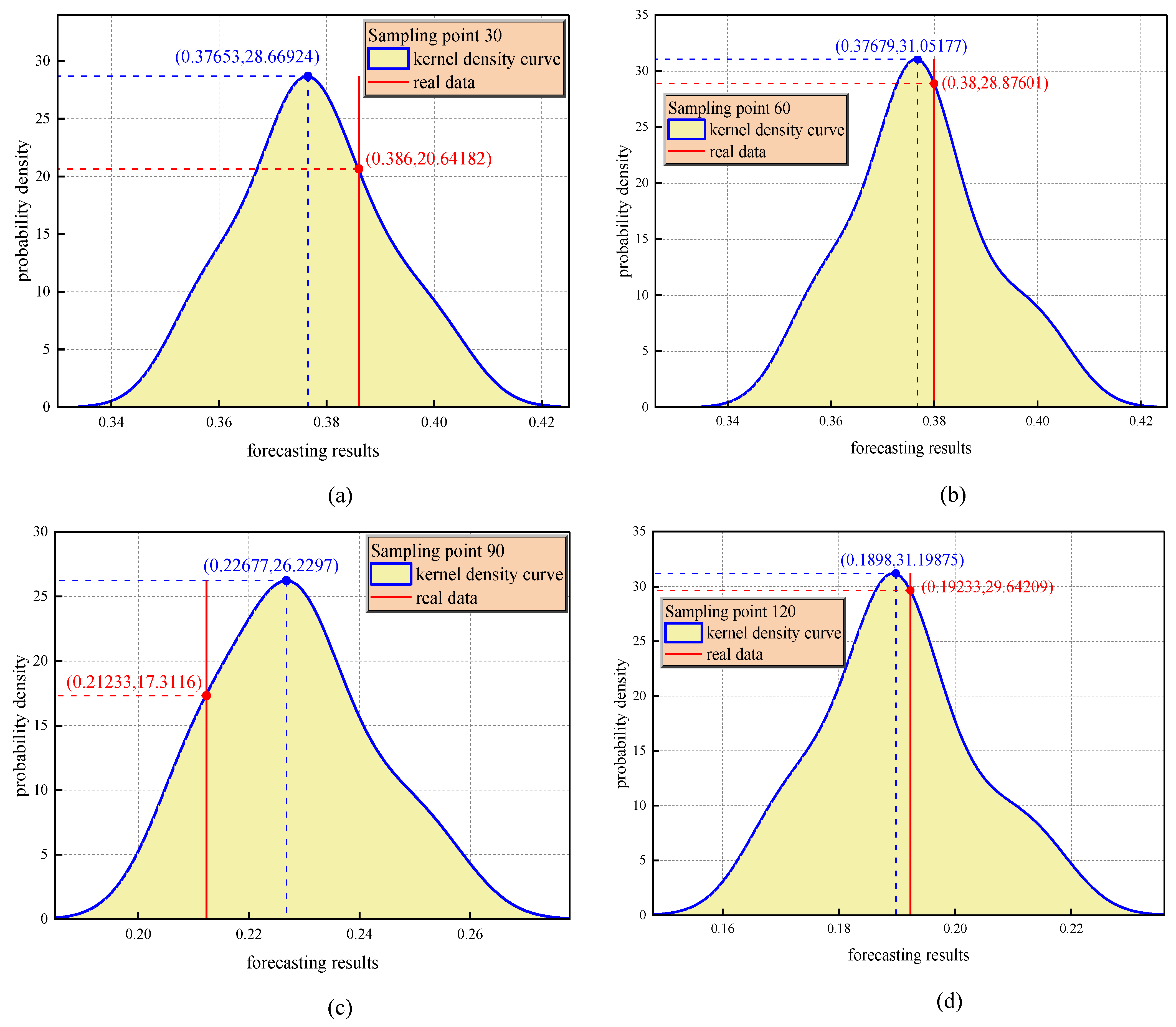
Figure 18a–d shows a comparison of the kernel density estimation curves for four sampling points (30, 60, 90, and 120) and reveals the time evolution law of error distribution prediction. The kernel density curve of each sampling point shows a significant unimodal characteristic, and its shape is visually consistent with the Gaussian distribution, indicating that the model can maintain a stable error distribution pattern at different stages of operation. Specifically, the peak density of sampling point 120 reaches 31.2 (corresponding to the mean error region), while the peak density of sampling point 90 decreases to 17.3. This difference in magnitude directly reflects the mean drift phenomenon of gas emission dynamics while the mine working face is being advanced.
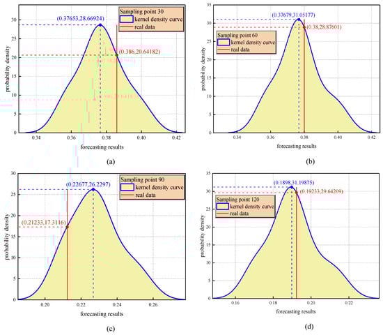
Figure 18.
(a–d) Prediction accuracy analysis for sampling points 30, 90, 60, and 120.
A quantitative comparison between the observed data and the predicted distribution shows that the actual concentration value (red solid line) has a systematic positive offset relative to the density peak at the sampling points of 30, 60, and 120, which is consistent with the low-frequency and high-amplitude characteristics of a sudden increase in gas concentration, indicating that the model has the ability to optimize the ability to capture low-frequency and high-amplitude abnormal events. It is worth noting that the actual concentration value of sampling point 90 is located in the right tail region of the predicted distribution, and its corresponding probability density is only 66% of the peak value, suggesting that the sensitivity of the model to extreme conditions needs to be improved.
3.6. Early Warning Mechanism for Gas Concentration Mutation Risk
The early warning mechanism for the risk of changes in coal mine gas concentration proposed in this study is based on two criteria: the dynamic confidence interval and kernel density distribution characteristics. With the combination of time series volatility quantification, probability distribution morphology analysis, and risk evolution trend prediction, an unsupervised intelligent early warning mechanism is realized by integrating time series volatility and probability density morphology. When the normalized average width () of the prediction interval exceeds two times the standard deviation of the historical mean (such as when the value at index 68 surges from a baseline of 0.16 to 0.28, an increase of 75%), the kernel density curve shows multi-peak distribution characteristics, and the evolution rate of the upper bound of the confidence interval breaks through the specific accelerated cumulative threshold, indicating that the fluctuation in gas concentration deviates significantly from the normal range, indicating an area with an abnormal risk of gas emission.
In Equations (27)–(29), represents the historical average width; represents the standard deviation, representing the statistical mean and the degree of dispersion; represents the gas timing cycle; represents the extreme point sequence of the kernel density estimation curve; and represents the upper bound function of the confidence interval.
The mechanism further introduces the evolution rate of the upper bound of the confidence interval as a trend prediction index to monitor the evolution of risk. When (such as the index 40–60 area), it indicates an accelerated cumulative gas concentration risk and that emergency ventilation must be started in advance. This early warning method, which is based on the combination of statistical distribution pattern analysis and dynamic trend quantification, overcomes the delay limitation of traditional threshold alarms. By upgrading the mode of risk identification from discrete threshold judgment to continuous probability space analysis, the technical improvement of the monitoring system from a passive alarm to active defense is realized.
4. Conclusions
4.1. Main Results
Aiming to eliminate the technical bottleneck of predicting gas concentration under complex conditions in deep mines, this study proposed an intelligent prediction and early warning system that combines spatio-temporal feature learning and uncertainty quantification. The main conclusions are as follows:
- (1)
- A TCN–Transformer hybrid architecture was proposed to capture the transient fluctuation characteristics of gas concentration through causal dilation convolution, and the long-range spatial–temporal correlation of geological–mining parameters was analyzed by incorporating the multi-head self-attention mechanism. The experiments showed that the model achieved a prediction accuracy of R2 = 0.980988 in measured data from Huangling Coal Mine, an improvement of 4.37% over the traditional TCN-GRU model.
- (2)
- CEC 2022 was used to verify the superior performance of the FLA, and a hyperparameter collaborative optimization framework based on the FLA was developed. The optimized parameters of the TCN–Transformer model, such as the number of filters (23) and the number of attention heads (8), significantly improved the model’s adaptability to non-stationary time series, and the MSE was reduced to 0.000114.
- (3)
- A local weighted regression kernel density estimation (LWD-KDE) method was proposed to achieve a 95% confidence interval coverage of 96.7%, while the normalized average interval width (PINAW) was compressed to 16.2%. A triple-pronged “interval width–density multi-peak–trend evolution” early warning mechanism was innovatively constructed, reducing the false negative rate under extreme working conditions.
4.2. Discussion
The coal mine gas prediction and early warning method proposed in this study, which is based on the TCN–Transformer structure, can respond rapidly to surges in gas concentration, but the interpretability, prediction accuracy, and timeliness of the model under non-steady-state conditions need to be improved. Future research will focus on achieving multi-source information fusion and model interpretability optimization by combining the Transformer architecture, dynamic graph neural network, and shape analysis.
Author Contributions
Conceptualization, Z.Y. and J.D.; methodology, L.Z.; software, L.Z.; validation, L.Z., Y.H. and Y.W. (Yanping Wang); formal analysis, Y.C.; investigation, Z.Q.; resources, J.D.; data curation, L.Z.; writing—original draft preparation, L.Z.; writing—review and editing, Z.Y.; visualization, Y.H.; supervision, J.D.; project administration, Z.Y. and Y.W. (Yiyang Wang); funding acquisition, J.D. All authors have read and agreed to the published version of the manuscript.
Funding
This research was funded by the Key Research and Development Program of Shaanxi Province, grant numbers 2022GY-150.
Data Availability Statement
The data are not publicly available due to commercial confidentiality, as they contain information that could compromise the privacy of research participants.
Acknowledgments
Thank you for the strong support of Xi’an University of Science and Technology platform, Yan Zhenguo and other members of the intelligent ventilation team research group.
Conflicts of Interest
The authors declare no conflicts of interest.
References
- Ni, K.; Feng, Y. Research on the safety development laws of coal mines in major coal-producing countries around the world. China Coal 2024, 50, 213–223. [Google Scholar] [CrossRef]
- Malozyomov, B.V.; Golik, V.I.; Brigida, V.; Kukartsev, V.V.; Tynchenko, Y.A.; Boyko, A.A.; Tynchenko, S.V. Substantiation of Drilling Parameters for Undermined Drainage Boreholes for Increasing Methane Production from Unconventional Coal-Gas Collectors. Energies 2023, 16, 4276. [Google Scholar] [CrossRef]
- Chang, H. Research on Coal Mine Longwall Face Gas State Analysis and Safety Warning Strategy Based on Multi-Sensor Forecasting Models. Sci. Rep. 2024, 14, 13795. [Google Scholar] [CrossRef]
- Nie, Y.; Wang, Y.; Wang, R. Coal and Gas Outburst Risk Prediction Based on the F-SPA Model. Energy Sources Part A Recovery Util. Environ. Eff. 2019, 45, 2717–2739. [Google Scholar] [CrossRef]
- Lu, J.; Jia, X.; Guo, X. Analysis on sensitive indicators of gas outburst based on improved gray prediction method. China Saf. Sci. J. 2022, 32, 74–81. [Google Scholar] [CrossRef]
- Ma, Y.; Chen, M. Identification of Gas Outburst Precursors Based on Outburst Percolation Theory. Sci. Rep. 2025, 15, 3228. [Google Scholar] [CrossRef]
- Dreger, M.; Celary, P. The Outburst Probability Index (Ww) as a New Tool in the Coal Seam Outburst Hazard Forecasting. J. Sustain. Min. 2024, 23, 55–60. [Google Scholar] [CrossRef]
- Anani, A.; Adewuyi, S.O.; Risso, N.; Nyaaba, W. Advancements in Machine Learning Techniques for Coal and Gas Outburst Prediction in Underground Mines. Int. J. Coal Geol. 2024, 285, 104471. [Google Scholar] [CrossRef]
- Tutak, M.; Krenicky, T.; Pirník, R.; Brodny, J.; Grebski, W.W. Predicting Methane Concentrations in Underground Coal Mining Using a Multi-Layer Perceptron Neural Network Based on Mine Gas Monitoring Data. Sustainability 2024, 16, 8388. [Google Scholar] [CrossRef]
- Liu, B.; Li, Z.; Zang, Z.; Yin, S.; Niu, Y.; Cai, M. Multi-Information Fusion Gas Concentration Prediction of Working Face Based on Informer. Min. Metall. Explor. 2025, 42, 597–613. [Google Scholar] [CrossRef]
- Shao, L.; Gao, Y. A Gas Prominence Prediction Model Based on Entropy-Weighted Gray Correlation and MCMC-ISSA-SVM. Processes 2023, 11, 2098. [Google Scholar] [CrossRef]
- Shao, L.; Chen, W. Coal and Gas Outburst Prediction Model Based on Miceforest Filling and PHHO–KELM. Processes 2023, 11, 2722. [Google Scholar] [CrossRef]
- Miao, D.; Ji, J.; Chen, X.; Lv, Y.; Liu, L.; Sui, X. Coal and Gas Outburst Risk Prediction and Management Based on WOA-ELM. Appl. Sci. 2022, 12, 10967. [Google Scholar] [CrossRef]
- Cai, Y.; Wu, S.; Zhou, M.; Gao, S.; Yu, H. Early Warning of Gas Concentration in Coal Mines Production Based on Probability Density Machine. Sensors 2021, 21, 5730. [Google Scholar] [CrossRef]
- Demirkan, D.C.; Duzgun, H.S.; Juganda, A.; Brune, J.; Bogin, G. Real-Time Methane Prediction in Underground Longwall Coal Mining Using AI. Energies 2022, 15, 6486. [Google Scholar] [CrossRef]
- Song, S.; Li, S.; Zhang, T.; Ma, L.; Pan, S.; Gao, L. Research on a Multi-Parameter Fusion Prediction Model of Pressure Relief Gas Concentration Based on RNN. Energies 2021, 14, 1384. [Google Scholar] [CrossRef]
- Liu, C.; Zhang, A.; Xue, J.; Lei, C.; Zeng, X. LSTM-Pearson Gas Concentration Prediction Model Feature Selection and Its Applications. Energies 2023, 16, 2318. [Google Scholar] [CrossRef]
- Kumari, K.; Dey, P.; Kumar, C.; Pandit, D.; Mishra, S.S.; Kisku, V.; Chaulya, S.K.; Ray, S.K.; Prasad, G.M. UMAP and LSTM Based Fire Status and Explosibility Prediction for Sealed-off Area in Underground Coal Mine. Process Saf. Environ. Prot. 2021, 146, 837–852. [Google Scholar] [CrossRef]
- Nguyen, T.-P. AIoT-Based Indoor Air Quality Prediction for Building Using Enhanced Metaheuristic Algorithm and Hybrid Deep Learning. J. Build. Eng. 2025, 105, 112448. [Google Scholar] [CrossRef]
- Lin, H.; Li, W.; Li, S.; Wang, L.; Ge, J.; Tian, Y.; Zhou, J. Coal Mine Gas Emission Prediction Based on Multifactor Time Series Method. Reliab. Eng. Syst. Saf. 2024, 252, 110443. [Google Scholar] [CrossRef]
- Dey, P.; Saurabh, K.; Kumar, C.; Pandit, D.; Chaulya, S.K.; Ray, S.K.; Prasad, G.M.; Mandal, S.K. T-SNE and Variational Auto-Encoder with a Bi-LSTM Neural Network-Based Model for Prediction of Gas Concentration in a Sealed-off Area of Underground Coal Mines. Soft Comput. 2021, 25, 14183–14207. [Google Scholar] [CrossRef]
- Xue, H.; Gui, X.; Wang, G.; Yang, X.; Gong, H.; Du, F. Prediction of Gas Drainage Changes from Nitrogen Replacement: A Study of a TCN Deep Learning Model with Integrated Attention Mechanism. Fuel 2024, 357, 129797. [Google Scholar] [CrossRef]
- Jia, P.; Liu, H.; Wang, S.; Wang, P. Research on a Mine Gas Concentration Forecasting Model Based on a GRU Network. IEEE Access 2020, 8, 38023–38031. [Google Scholar] [CrossRef]
- Vaswani, A.; Shazeer, N.; Parmar, N.; Uszkoreit, J.; Jones, L.; Gomez, A.N.; Kaiser, Ł.; Polosukhin, I. Attention Is All You Need. Adv. Neural Inf. Process Syst. 2017, 30. [Google Scholar] [CrossRef]
- Yang, H.; Wang, J.; Zhang, H. Research on Gas Multi-Indicator Warning Method of Coal Mine Working Face Based on MOA-Transformer. ACS Omega 2024, 9, 22136–22144. [Google Scholar] [CrossRef]
- Yan, Z.; Qin, Z.; Fan, J.; Huang, Y.; Wang, Y.; Zhang, J.; Zhang, L.; Cao, Y. Gas Outburst Warning Method in Driving Faces: Enhanced Methodology through Optuna Optimization, Adaptive Normalization, and Transformer Framework. Sensors 2024, 24, 3150. [Google Scholar] [CrossRef]
- Wang, X.; Xu, N.; Meng, X.; Chang, H. Prediction of Gas Concentration Based on LSTM-LightGBM Variable Weight Combination Model. Energies 2022, 15, 827. [Google Scholar] [CrossRef]
- Liang, Y.; Li, S.; Li, Q.; Guo, Y.; Sun, W.; Zheng, M.; Wang, C. Prediction of Gas Concentration in the Upper Corner of Mining Working Face Based on the FEDformer-LGBM-AT Architecture. J. China Coal Soc. 2025, 50, 360–378. [Google Scholar] [CrossRef]
- Zhang, Y.; Chen, H.C.; Du, Y.; Chen, M.; Liang, J.; Li, J.; Fan, X.; Sun, L.; Cheng, Q.S.; Yao, X. Early Warning of Incipient Faults for Power Transformer Based on DGA Using a Two-Stage Feature Extraction Technique. IEEE Trans. Power Deliv. 2021, 37, 2040–2049. [Google Scholar] [CrossRef]
- Zou, H.; Hastie, T.; Tibshirani, R. Sparse Principal Component Analysis. J. Comput. Graph. Stat. 2006, 15, 265–286. [Google Scholar] [CrossRef]
- Xu, Y.; Cheng, Y. Prediction of coal and gas outburst risk based on SKPCA and NEAT algorithm. J. Saf. Environ. 2021, 21, 1427–1433. [Google Scholar] [CrossRef]
- Zhao, H.; Gong, Z.; Gan, K.; Gan, Y.; Xing, H.; Wang, S. Supervised Kernel Principal Component Analysis-Polynomial Chaos-Kriging for High-Dimensional Surrogate Modelling and Optimization. Knowl.-Based Syst. 2024, 305, 112617. [Google Scholar] [CrossRef]
- Ghasemi, M.; Golalipour, K.; Zare, M.; Mirjalili, S.; Trojovský, P.; Abualigah, L.; Hemmati, R. Flood Algorithm (FLA) an Efficient Inspired Meta. J. Supercomput. 2024, 80, 22913–23017. [Google Scholar] [CrossRef]
- Gao, J.; Cheng, Y.; Zhang, D.; Chen, Y. Physics-Constrained Wind Power Forecasting Aligned with Probability Distributions for Noise-Resilient Deep Learning. Appl. Energy 2025, 383, 125295. [Google Scholar] [CrossRef]
- Su, Q.; Lu, H.; Yin, X.; Lu, Q.; Yan, J. Hybrid Point-Interval Prediction Method for Stochastic Dynamic Response of Subsea Umbilical Cable Based on BO-BiLSTM and Adaptive Bandwidth KDE. Ocean. Eng. 2025, 320, 120317. [Google Scholar] [CrossRef]


Disclaimer/Publisher’s Note: The statements, opinions and data contained in all publications are solely those of the individual author(s) and contributor(s) and not of MDPI and/or the editor(s). MDPI and/or the editor(s) disclaim responsibility for any injury to people or property resulting from any ideas, methods, instructions or products referred to in the content. |
© 2025 by the authors. Licensee MDPI, Basel, Switzerland. This article is an open access article distributed under the terms and conditions of the Creative Commons Attribution (CC BY) license (https://creativecommons.org/licenses/by/4.0/).