
Investigation of Various Fire Dynamics Simulator Approaches to Modelling Airflow in Road Tunnel Induced by Longitudinal Ventilation


Abstract
1. Introduction
2. Materials and Methods
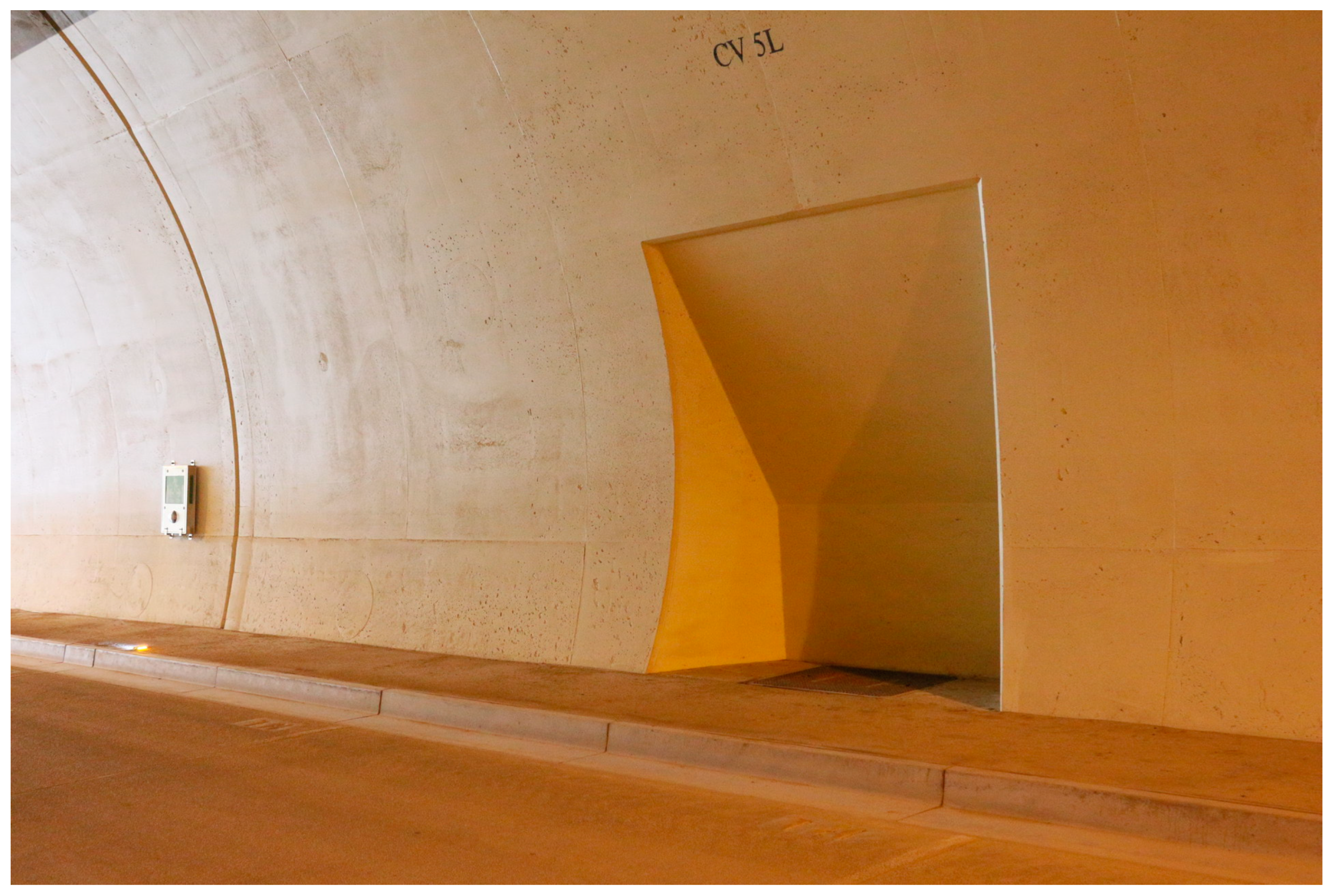
2.1. Ventilation Tests in the Polana Tunnel
2.2. FDS Modelling of the Polana Tunnel
2.3. Determination of Free Parameters of the Models
3. Results and Discussion
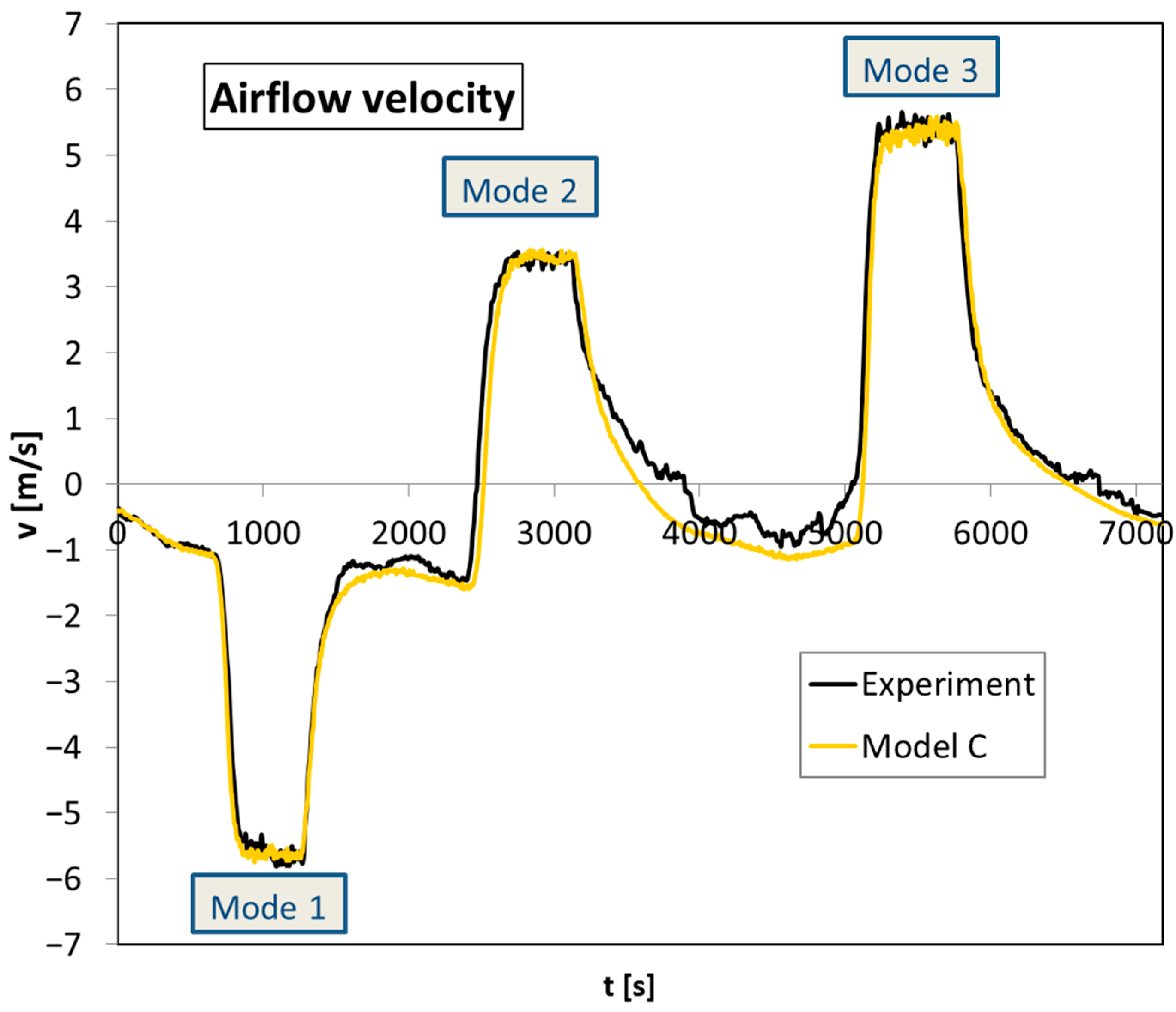
3.1. Airflow Velocity Evaluation
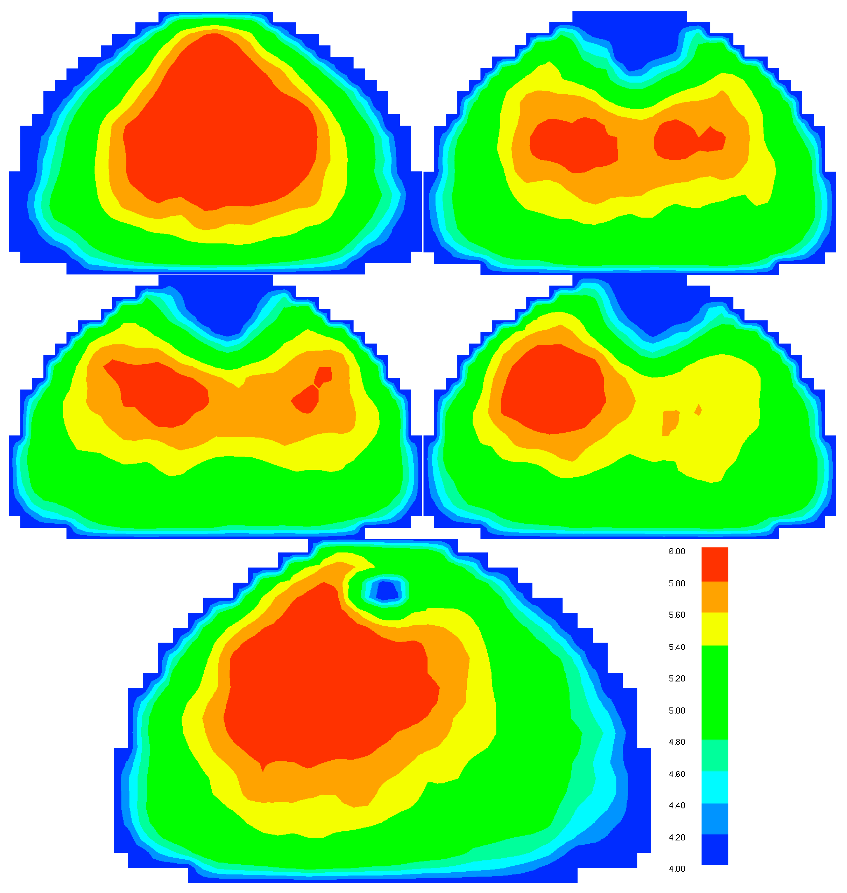
3.2. Airflow Velocity Profile
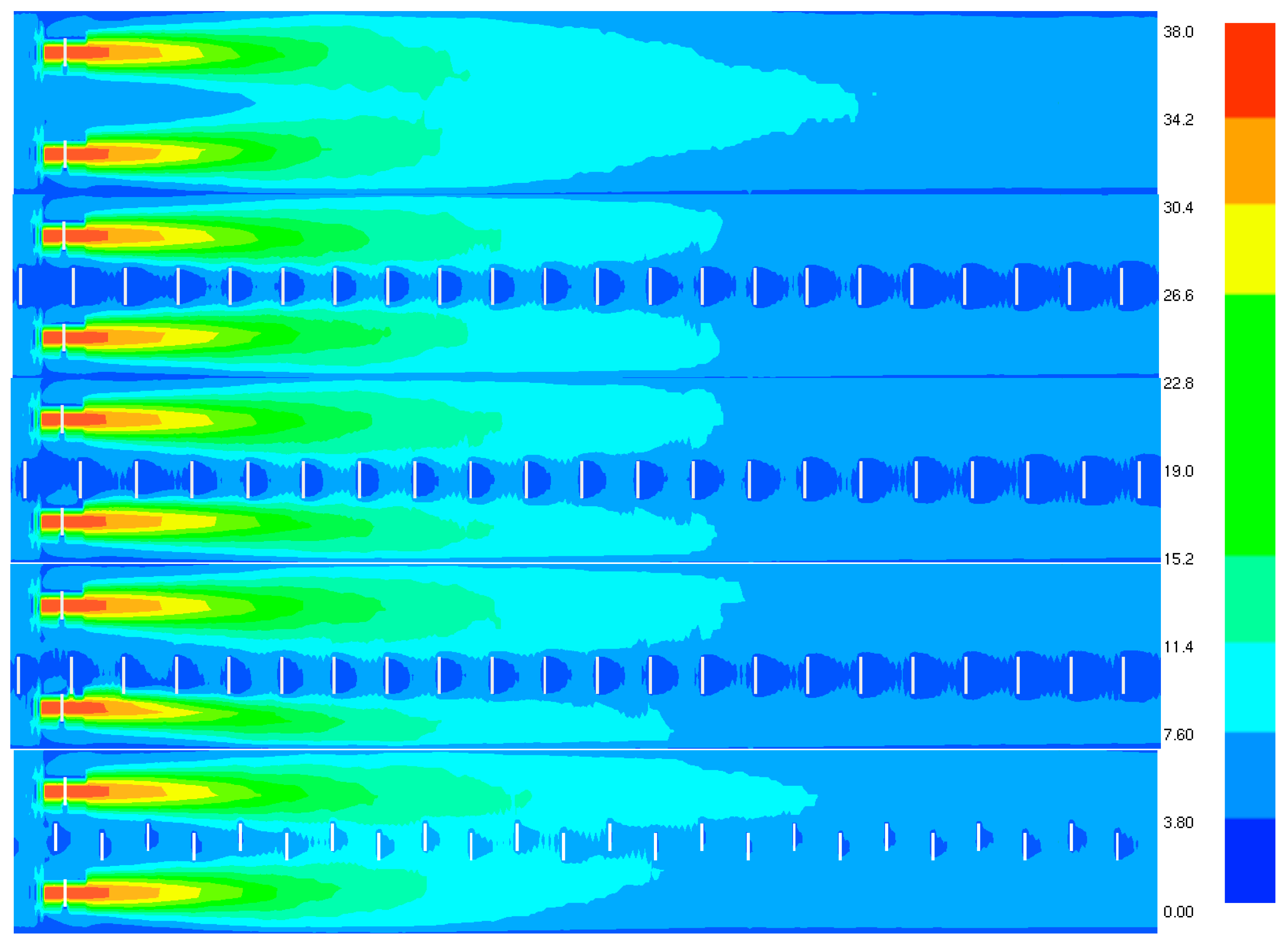
3.3. Velocity Profile and Velocity Distribution Visualization
3.4. Airflow Velocities Measured by Tunnel Anemometers
3.5. Simulation Performance
4. Conclusions
Author Contributions
Funding
Institutional Review Board Statement
Informed Consent Statement
Data Availability Statement
Acknowledgments
Conflicts of Interest
References
- McGrattan, K.; Hostikka, S.; McDermott, R.; Floyd, J.; Weinschenk, C.; Overholt, K. Fire Dynamics Simulator, Technical Reference Guide, 6th ed.; NIST and VTT Technical Research Centre of Finland: Espoo, Finland, 2017. [Google Scholar]
- McGrattan, K.; Hostikka, S.; McDermott, R.; Floyd, J.; Weinschenk, C.; Overholt, K. Fire Dynamics Simulator, User’s Guide, 6th ed.; NIST and VTT Technical Research Centre of Finland: Espoo, Finland, 2017. [Google Scholar]
- Deckers, X.; Haga, S.; Tilley, N.; Merci, B. Smoke control in case of fire in a large car park: CFD simulations of full-scale configurations. Fire Saf. J. 2013, 57, 22–34. [Google Scholar] [CrossRef]
- Valasek, L.; Glasa, J. On Realization of Cinema Hall Fire Simulation Using Fire Dynamics Simulator. Comput. Inform. 2017, 36, 971–1000. [Google Scholar] [CrossRef]
- Kim, E.; Woycheese, J.P.; Dembsey, N.A. Fire dynamics simulator (Version 4.0) simulation for tunnel fire scenarios with forced, transient, longitudinal ventilation flows. Fire Technol. 2008, 44, 137–166. [Google Scholar] [CrossRef]
- Álvarez-Coedo, D.; Ayala, P.; Cantizano, A.; Węgrzyński, W. A coupled hybrid numerical study of tunnel longitudinal ventilation under fire conditions. Case Stud. Therm. Eng. 2022, 36, 102202. [Google Scholar] [CrossRef]
- Zisis, T.; Vasilopoulos, K.; Sarris, I. Numerical simulation of a fire accident in a longitudinally ventilated railway tunnel and tenability analysis. Appl. Sci. 2022, 12, 5667. [Google Scholar] [CrossRef]
- Weng, M.C.; Yu, L.X.; Liu, F.; Nielsen, P.V. Full-scale experiment and CFD simulation on smoke movement and smoke control in a metro tunnel with one opening portal. Tunn. Undergr. Space Technol. 2014, 42, 96–104. [Google Scholar] [CrossRef]
- Hsu, W.-S.; Huang, Y.-H.; Shen, T.-S.; Cheng, C.-Y.; Chen, T.-Y. Analysis of the Hsuehshan Tunnel Fire in Taiwan. Tunn. Undergr. Space Technol. 2017, 69, 108–115. [Google Scholar] [CrossRef]
- Du, T.; Li, P.; Wei, H.; Yang, D. On the backlayering length of the buoyant smoke in inclined tunnel fires under natural ventilation. Case Stud. Therm. Eng. 2022, 39, 102455. [Google Scholar] [CrossRef]
- Zhang, X.; Lin, Y.; Shi, C.; Zhang, J. Numerical simulation on the maximum temperature and smoke back-layering length in a tilted tunnel under natural ventilation. Tunn. Undergr. Space Technol. 2022, 107, 103661. [Google Scholar] [CrossRef]
- Ang, C.D.; Rein, G.; Peiro, J.; Harrison, R. Simulating longitudinal ventilation flows in long tunnels: Comparison of full CFD and multi-scale modelling approaches in FDS6. Tunn. Undergr. Space Technol. 2016, 52, 119–126. [Google Scholar] [CrossRef]
- Król, A.; Król, M.; Koper, P.; Wrona, P. Numerical modeling of air velocity distribution in a road tunnel with a longitudinal ventilation system. Tunn. Undergr. Space Technol. 2019, 91, 103003. [Google Scholar] [CrossRef]
- Brzezińska, D. Practical aspects of jet fan ventilation systems modelling in fire dynamics simulator code. Int. J. Vent. 2018, 17, 225–239. [Google Scholar] [CrossRef]
- Brzezinska, D.; Sompolinski, M. The accuracy of mapping the airstream of jet fan ventilators by fire dynamics simulator. Sci. Technol. Built Environ. 2017, 23, 736–747. [Google Scholar] [CrossRef]
- Król, A.; Król, M. some tips on numerical modeling of airflow and fires in road tunnels. Energies 2021, 14, 2366. [Google Scholar] [CrossRef]
- Król, A.; Król, M. Study on numerical modeling of jet fans. Tunn. Undergr. Space Technol. 2018, 73, 222–235. [Google Scholar] [CrossRef]
- Weisenpacher, P.; Valasek, L. Computer simulation of airflows generated by jet fans in real road tunnel by parallel version of FDS 6. Int. J. Vent. 2021, 20, 20–33. [Google Scholar] [CrossRef]
- Pope, S.B. Turbulent Flows; Cambridge University Press: Cambridge, UK, 2000. [Google Scholar]
- Weisenpacher, P. Modeling of road tunnel airflows by FDS using tunnel model with a system of geometrical objects. In Proceedings of the 35rd European Modeling and Simulation Symposium (EMSS 2023), Athens, Greece, 18–20 September 2023. [Google Scholar] [CrossRef]
- Pospisil, P.; Ockajak, R. Tunel Polana—DRS Vetranie Tunela a Unikovej Stolne; Technical Report; IP Engineering GmbH: Munchenstein, Switzerland, 2016. [Google Scholar]
- Danišovič, P.; Šrámek, J.; Hodoň, M.; Húdik, M. Testing measurements of airflow velocity in road tunnels. MATEC Web Conf. 2017, 117, 00035. [Google Scholar] [CrossRef]
- Pospisil, P.; Ockajak, R. Skusky Vetrania Tunela Polana a Svrcinovec; Technical Report; IP Engineering GmbH: Munchenstein, Switzerland, 2017. [Google Scholar]
- Glasa, J.; Valasek, L.; Weisenpacher, P.; Kubisova, T. Improvement of modeling velocity of airflow created by emergency ventilation in a road tunnel using FDS 6. Appl. Sci. 2023, 13, 2762. [Google Scholar] [CrossRef]
- Beyer, M.; Sturm, P.-J.; Sauerwein, M.; Bacher, M. Evaluation of Jet Fan Performance in Tunnels. In IVT Reports: Proceedings Tunnel Safety and Ventilation; Verlag der Technischen Universität Graz: Graz, Austria, 2016; Volume 100, p. 298. [Google Scholar]
- Chen, T.; Zhou, D.; Lu, Z.; Li, Y.; Xu, Z.; Wang, B.; Fan, C. Study of the applicability and optimal arrangement of alternative jet fans in curved road tunnel complexes. Tunn. Undergr. Space Technol. 2021, 108, 103721. [Google Scholar] [CrossRef]
- Wang, F.; Wang, M.; He, S.; Zhang, J.; Deng, Y. Computational study of effects of jet fans on the ventilation of a highway curved tunnel. Tunn. Undergr. Space Technol. 2010, 25, 382–390. [Google Scholar] [CrossRef]
- nscc.sk. Available online: https://userdocs.nscc.sk/devana/system_overview/ (accessed on 10 August 2024).


| Fan wheel diameter | 0.8 m |
| Length of shroud | 3.7 m |
| Maximal volume flow | 19 m3·s−1 |
| Maximal velocity at fan exit | 38.5 m·s−1 |
| Thrust | 850 N |
| Location | 101, 201, 716, and 801 m from the west portal at a height of 5.1 m |
| Jet Fan Power | Direction | |
|---|---|---|
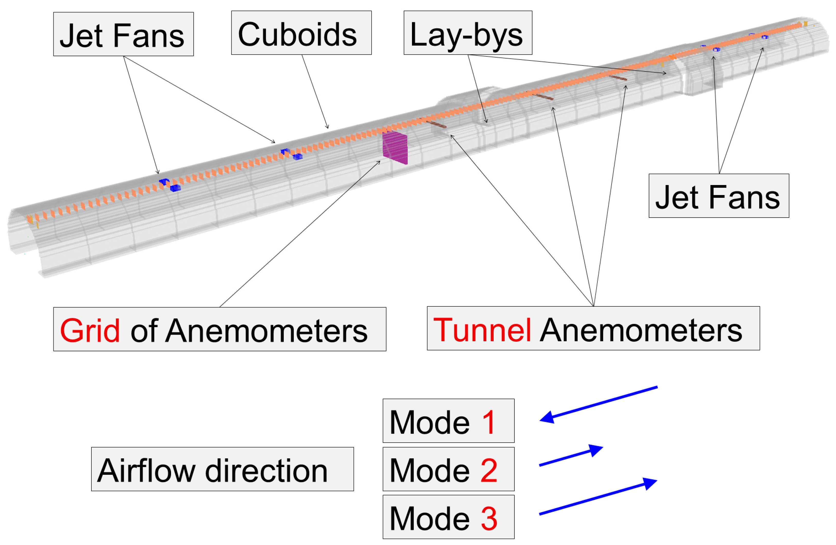
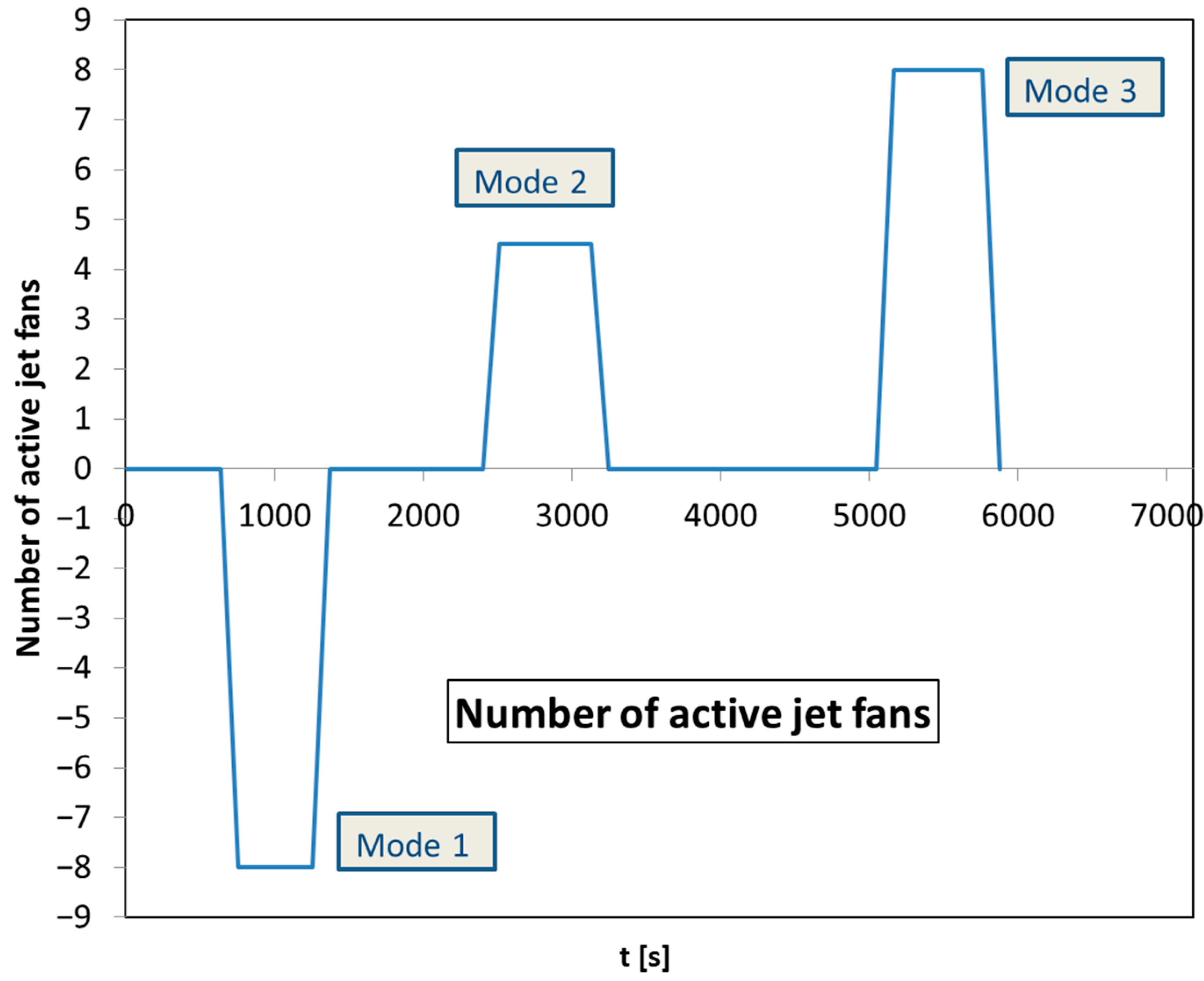
| Mode 1 | 8 jet fans: 100% | Westward |
| Mode 2 | 3 jet fans: 100% 5 jet fans: 30% | Eastward |
| Mode 3 | 8 jet fans: 100% | Eastward |
| Accuracy | Recording Frequency | Location | |
|---|---|---|---|
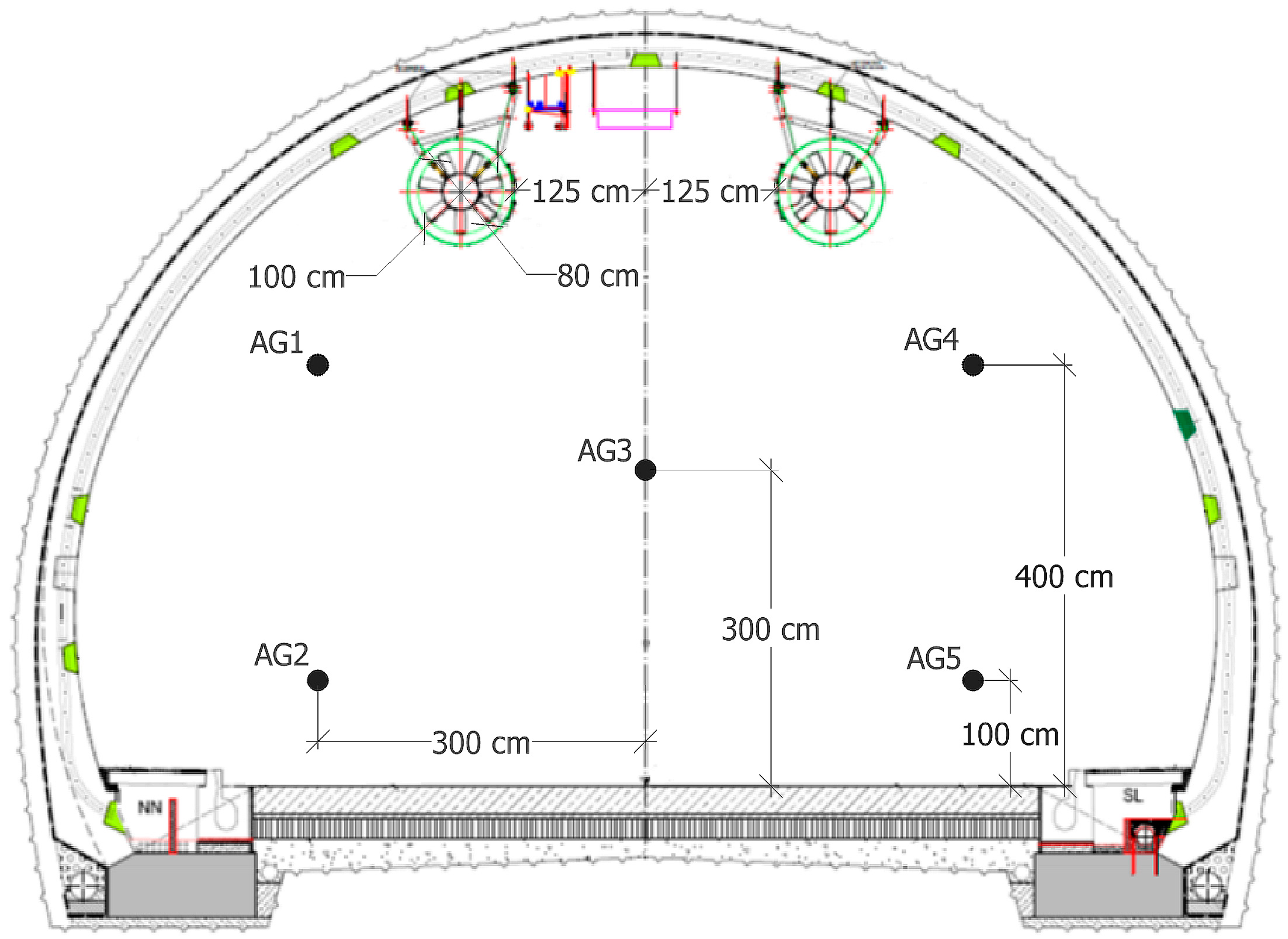
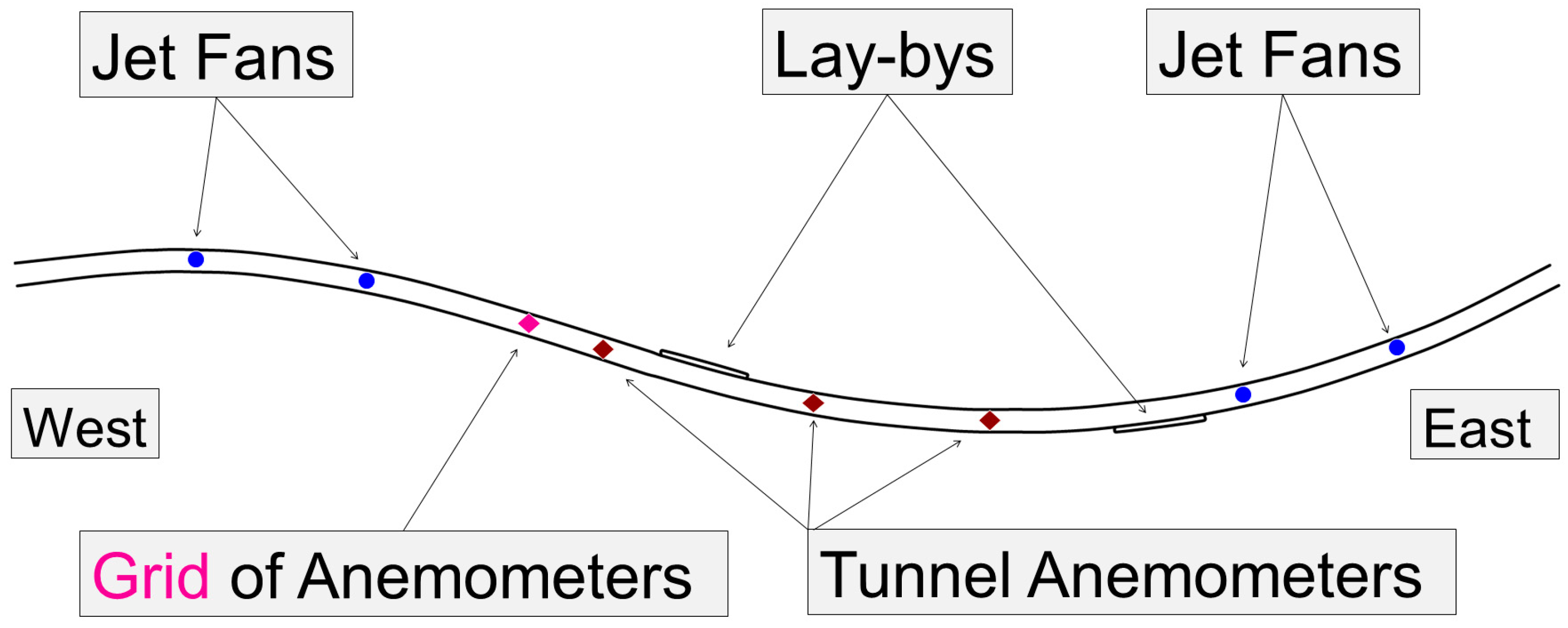
| AG1–5 | 0.3 m·s−1 | 5 s | 300 m, Figure 1 and Figure 2 |
| AT1–3 | 0.1 m·s−1 | 5 s | 340, 465, 565 m, Figure 2 |
| Ambient temperature | 6 °C |
| Mesh resolution | 30 cm |
| Computational domain | 900 × 18 × 8.1 m |
| Mesh decomposition | 12 × 1 × 1 (12 identical meshes) |
| Cells | 3000 × 60 × 27 (4,860,000 total) |
| Cells per mesh | 250 × 60 × 27 (405,000 total) |
| Turbulence | LES, Deardorff model |
| Boundary conditions | CONCRETE for tunnel walls, OPEN with prescribed dynamic pressure for tunnel portals |
| Dynamic pressure | Variable, from −6.3 to −1 Pa [18] |
| Time step | Variable, typically 6·10−3 s for active jet fans |
| Simulation time | 7180 s |
| Simulation elapsed time | 458 hrs (A1), 450 hrs (A2), 453 hrs (S), 469 hrs (C) |
| Settings | Cuboids | RMSD3 | RMSD15 |
|---|---|---|---|
| 1 | 160 | 0.162 | 0.579 |
| 2 | 166 | 0.113 | 0.581 |
| 3 | 170 | 0.115 | 0.531 |
| 4 | 174 | 0.081 | 0.536 |
| 5 | 178 | 0.029 | 0.524 |
| Settings | εH | Cuboids | RMSD3 | RMSD15 |
|---|---|---|---|---|
| 1 | 160 | 334 | 0.053 | 0.445 |
| 2 | 200 | 300 | 0.115 | 0.458 |
| 3 | 200 | 200 | 0.036 | 0.441 |
| 4 | 250 | 150 | 0.037 | 0.450 |
| S | 173 cuboids (1 × 4 × 3 cells) above centreline, 5.1 m mutual distance |
| A1 | 83 cuboids (1 × 4 × 3 cells) shifted to the right, 83 cuboids shifted to the left, 5.4 m mutual distance |
| A2 | 89 cuboids (1 × 4 × 3 cells) shifted to the right, 89 cuboids shifted to the left, 5.1 m mutual distance |
| C | Roughness: εH = 0.200 m (convex walls), εL = 0.003 m (all other surfaces), 200 cuboids (1 × 3 × 1 cells), 4.5 m mutual distance |
| Mode 1 | Mode 2 | Mode 3 | RMSD3 | RMSD15 | ||||
|---|---|---|---|---|---|---|---|---|
| Experiment | −5.61 | 3.42 | 5.41 | |||||
| Model 0 | −5.72 | 2.1% | 3.47 | 1.5% | 5.43 | 0.3% | 0.074 | 0.593 |
| Model S | −5.69 | 1.5% | 3.45 | 1.0% | 5.44 | 0.7% | 0.057 | 0.518 |
| Model A1 | −5.68 | 1.2% | 3.48 | 1.8% | 5.48 | 1.4% | 0.069 | 0.522 |
| Model A2 | −5.64 | 0.6% | 3.41 | −0.1% | 5.44 | 0.7% | 0.029 | 0.524 |
| Model C | −5.63 | 0.5% | 3.45 | 1.1% | 5.37 | −0.8% | 0.036 | 0.441 |
| AG1 | AG2 | AG3 | AG4 | AG5 | MAPD5 | Max5 | |
|---|---|---|---|---|---|---|---|
| Experiment | −5.19 | −5.39 | −6.09 | −5.53 | −5.83 | ||
| Model 0 | −5.41 | −5.64 | −6.29 | −5.56 | −5.71 | ||
| 4.2% | 4.6% | 3.4% | 0.5% | −2.1% | 3.0% | 4.6% | |
| Model S | −5.32 | −5.65 | −5.98 | −5.48 | −6.04 | ||
| 2.3% | 4.8% | −1.8% | −0.9% | 3.6% | 2.7% | 4.8% | |
| Model A1 | −5.30 | −5.65 | −5.97 | −5.44 | −6.03 | ||
| 2.1% | 4.7% | −1.9% | −1.6% | 3.3% | 2.7% | 4.7% | |
| Model A2 | −5.37 | −5.64 | −5.91 | −5.36 | −5.94 | ||
| 3.3% | 4.5% | −2.9% | −3.1% | 1.9% | 3.1% | 4.5% | |
| Model C | −5.57 | −5.48 | −5.85 | −5.61 | −5.66 | ||
| 7.2% | 1.6% | −3.8% | 1.4% | −2.9% | 3.4% | 7.2% |
| AG1 | AG2 | AG3 | AG4 | AG5 | MAPD5 | Max5 | |
|---|---|---|---|---|---|---|---|
| Experiment | 3.30 | 3.40 | 3.59 | 3.55 | 3.25 | ||
| Model 0 | 3.21 | 3.37 | 3.93 | 3.41 | 3.42 | ||
| −2.5% | −0.9% | 9.4% | −3.9% | 5.2% | 4.4% | 9.4% | |
| Model S | 3.40 | 3.38 | 3.61 | 3.42 | 3.45 | ||
| 3.1% | −0.6% | 0.6% | −3.7% | 6.3% | 2.9% | 6.3% | |
| Model A1 | 3.48 | 3.43 | 3.67 | 3.35 | 3.47 | ||
| 5.5% | 0.9% | 2.1% | −5.7% | 6.9% | 4.2% | 6.9% | |
| Model A2 | 3.51 | 3.36 | 3.63 | 3.21 | 3.37 | ||
| 6.3% | −1.3% | 1.1% | −9.6% | 3.8% | 4.4% | 9.6% | |
| Model C | 3.60 | 3.47 | 3.81 | 3.19 | 3.20 | ||
| 9.1% | 2.1% | 6.1% | −10.0% | −1.5% | 5.8% | 10.0% |
| AG1 | AG2 | AG3 | AG4 | AG5 | MAPD5 | Max5 | |
|---|---|---|---|---|---|---|---|
| Experiment | 5.93 | 6.55 | 5.53 | 4.87 | 4.16 | ||
| Model 0 | 5.23 | 4.96 | 6.34 | 5.51 | 5.09 | ||
| −11.7% | −24.3% | 14.6% | 13.2% | 22.2% | 17.2% | 24.3% | |
| Model S | 5.54 | 5.14 | 5.70 | 5.67 | 5.18 | ||
| −6.6% | −21.4% | 3.0% | 16.4% | 24.4% | 14.4% | 24.4% | |
| Model A1 | 5.70 | 5.16 | 5.61 | 5.71 | 5.23 | ||
| −3.8% | −21.2% | 1.4% | 17.3% | 25.7% | 13.9% | 25.7% | |
| Model A2 | 5.70 | 5.12 | 5.59 | 5.53 | 5.28 | ||
| −3.8% | −21.8% | 1.1% | 13.5% | 26.8% | 13.4% | 26.8% | |
| Model C | 5.69 | 5.24 | 5.98 | 5.15 | 4.77 | ||
| −4.0% | −20.0% | 8.0% | 5.8% | 14.6% | 10.5% | 20.0% |
| Mode 1 | Mode 2 | Mode3 | ||||
|---|---|---|---|---|---|---|
| Experiment | −5.15 | 3.24 | 5.08 | |||
| Model S | −4.96 | −3.8% | 2.91 | −10.1% | 4.79 | −5.8% |
| Model C | −5.19 | 0.8% | 3.17 | −2.1% | 5.18 | 2.0% |
| Meshes | Number of Meshes | Cells in Mesh | Number of Cells in Mesh | Tunnel Region | Section |
|---|---|---|---|---|---|
| 1–17 | 17 | 50 × 40 × 24 | 48,000 | [0.0, 255.0] | A |
| 18–25 | 8 | 49 × 40 × 24 | 47,040 | [255.0, 372.6] | |
| 26–30 | 5 | 34 × 50 × 27 | 45,900 | [372.6, 423.6] | B |
| 31–39 | 9 | 50 × 40 × 24 | 48,000 | [423.6, 558.6] | C |
| 40–44 | 5 | 51 × 40 × 24 | 48,960 | [558.6, 635.1] | |
| 45–49 | 5 | 34 × 50 × 27 | 45,900 | [635.1, 686.1] | D |
| 50–56 | 7 | 47 × 40 × 24 | 45,120 | [686.1, 784.8] | E |
| 57–64 | 8 | 48 × 40 × 24 | 46,080 | [784.8, 900.0] | |
| Total | 64 | 3,012,600 | [0.0, 900.0] |
| Mode 1 Velocity [m·s−1] | Mode 1 Velocity [m·s−1] | Mode 1 Velocity [m·s−1] | RMSD3 [m·s−1] | RMSD15 [m·s−1] | Wall Clock Time [hrs] | Speedup | |
|---|---|---|---|---|---|---|---|
| Experiment | −5.61 | 3.42 | 5.41 | ||||
| SIVVP, 12 M | −5.63 | 3.45 | 5.37 | 0.036 | 0.441 | 469 | |
| 0.5% | 1.1% | −0.8% | |||||
| Devana, 12 M | −5.62 | 3.48 | 5.38 | 0.038 | 0.438 | 157 | 3.0 |
| 0.2% | 1.7% | −0.4% | |||||
| Devana, 64 M | −5.68 | 3.48 | 5.45 | 0.061 | 0.430 | 36 | 13.1 |
| 1.3% | 2.0% | 0.7% |
Disclaimer/Publisher’s Note: The statements, opinions and data contained in all publications are solely those of the individual author(s) and contributor(s) and not of MDPI and/or the editor(s). MDPI and/or the editor(s) disclaim responsibility for any injury to people or property resulting from any ideas, methods, instructions or products referred to in the content. |
© 2025 by the authors. Licensee MDPI, Basel, Switzerland. This article is an open access article distributed under the terms and conditions of the Creative Commons Attribution (CC BY) license (https://creativecommons.org/licenses/by/4.0/).
Share and Cite
Weisenpacher, P.; Glasa, J.; Valasek, L. Investigation of Various Fire Dynamics Simulator Approaches to Modelling Airflow in Road Tunnel Induced by Longitudinal Ventilation. Fire 2025, 8, 74. https://doi.org/10.3390/fire8020074
Weisenpacher P, Glasa J, Valasek L. Investigation of Various Fire Dynamics Simulator Approaches to Modelling Airflow in Road Tunnel Induced by Longitudinal Ventilation. Fire. 2025; 8(2):74. https://doi.org/10.3390/fire8020074
Chicago/Turabian StyleWeisenpacher, Peter, Jan Glasa, and Lukas Valasek. 2025. "Investigation of Various Fire Dynamics Simulator Approaches to Modelling Airflow in Road Tunnel Induced by Longitudinal Ventilation" Fire 8, no. 2: 74. https://doi.org/10.3390/fire8020074
APA StyleWeisenpacher, P., Glasa, J., & Valasek, L. (2025). Investigation of Various Fire Dynamics Simulator Approaches to Modelling Airflow in Road Tunnel Induced by Longitudinal Ventilation. Fire, 8(2), 74. https://doi.org/10.3390/fire8020074