Development of a Combustible Material Pyrolysis Model for Ultra-Fast Analysis: A Study on the Behavior of Ultra-Fast Fire in Industrial Complexes

Abstract

This study develops a combustible material pyrolysis model capable of numerically predicting and analyzing ultra-fast fire scenarios. The model was subsequently applied to investigate fire behavior in industrial complex facilities. Based on a propolis model and a User-Defined Function (UDF), the proposed approach simulated the mass loss of specimens due to pyrolysis and combustion, and the results were compared with experimental data. A strong correlation confirmed the reliability of the model. Using this validated framework, flame propagation patterns under various fire scenarios were analyzed, providing a quantitative characterization of the thermal behavior and propagation mechanisms of ultra-fast fires in industrial complexes.

1. Introduction

Industrial complexes are characterized by the concentration of numerous enterprises and diverse facilities. Most factory buildings employ prefabricated sandwich panels as their primary structural components to ensure construction efficiency and economic feasibility. While sandwich panels offer advantages such as rapid construction and cost reduction, they have the critical drawback of being far more vulnerable to fire compared with conventional reinforced concrete structures. In particular, when a fire breaks out in an industrial complex where large amounts of hazardous materials and gases are handled, the damage can quickly extend beyond a single facility, spreading to neighboring buildings and potentially escalating into a large-scale urban fire [1,2,3,4]. As illustrated by recent cases—including the fire at the Aricell’s lithium battery factory (2024), the Fire at Cheonan Auto Parts Factory (2025), and the fire at Kumho Tire’s Gwangju plant (2025)—the high density of buildings within industrial complexes contributes to rapid fire spread. Furthermore, hazardous substances released during such events can inflict severe harm on human health and the environment [5,6,7].

To mitigate these risks and enhance the fire safety of buildings, Korean regulations require that structures with a total floor area exceeding 1000 m² be compartmentalized using fire-resistant floors, walls, fire doors, or automatic fire shutters. The performance of these fire-resistant assemblies is evaluated according to standardized fire heating curves, such as ISO 834 [8] and KS F 2257 [9], which define temperature rise conditions over time. However, fires occurring in industrial complexes often deviate significantly from typical fire scenarios. In particular, ultra-fast fires—characterized by a rapid release of heat, with the heat release rate (HRR) reaching 1 MW within just one minute—can develop. Such sudden energy release produces fire conditions far more severe than those represented by standardized curves, making it difficult to ensure structural safety under existing criteria.

Moreover, research on ultra-fast fires remains in its infancy. Current studies primarily focus on HRR as a function of time, without establishing clear definitions or application boundaries. This gap complicates efforts to accurately characterize actual fire behavior in industrial complexes and to design effective structural and fire protection strategies.

In addition, although full-scale fire experiments can provide high-fidelity insight into fire dynamics and structural response, they are often constrained by excessive costs, time consumption, pollutant generation, and significant safety concerns—factors that limit their widespread applicability. Consequently, computational fluid dynamics (CFD) modeling has emerged as a practical alternative to large-scale testing, enabling detailed investigation of flame propagation and thermal behavior under various scenarios. For example, CFD simulations using the SMARTFIRE program were conducted to reproduce large-scale aircraft fire experiments carried out by the Federal Aviation Administration (FAA), successfully predicting the flashover time with only a 10 s deviation from the experimental result, thereby demonstrating the predictive capability of the model [10]. A separate numerical study reconstructed the 2022 fire accident of the Wan’an Bridge—a timber bridge—using the Fire Dynamics Simulator (FDS), showing that while the simulation reproduced the overall flame spread patterns, it tended to underestimate the propagation rate due to limitations in representing accidental ignition conditions [11]. Another investigation employed FDS to analyze flame spread from LED screens installed on building façades, utilizing experimentally derived heat release rate per unit area (HRRPUA) curves from ASTM tests to account for variations in polymer composition among manufacturers. The results indicated that combining standardized test data with CFD modeling provides a cost-effective engineering approach for predicting façade fire behavior [12]. In addition, a customized pyrolysis model (Pyropolis model) was developed to simulate ignition and combustion of solid samples exposed to Bunsen burner flames. When coupled with ANSYS Fluent 2023 R2 (version 23.2), the model demonstrated good agreement with benchmark experiments such as UL 94 and VBB tests, suggesting that CFD-based pyrolysis simulations can reliably replicate standard fire test conditions [13,14].

Therefore, this study develops a combustible material pyrolysis model capable of analyzing ultra-fast fire behavior and applies it to industrial facilities. The pyrolysis model for solid combustibles was derived based on the Arrhenius law, numerically resolving mass and heat transfer between solid fuels and the gaseous domain. In the gas phase, conservation equations for mass, momentum, and energy, as well as the ideal gas law and species transport equations, were considered. The analysis was conducted using ANSYS Fluent in combination with User-Defined Functions (UDFs). Model reliability was verified by comparing numerical results with experimental data obtained from Microscale Combustion Calorimetry (MCC) [13]. The validated model was then applied to investigate ultra-fast fire characteristics under various fire scenarios in industrial facilities.

2. Vertical Flame Propagation Experiment Using a Bunsen Burner

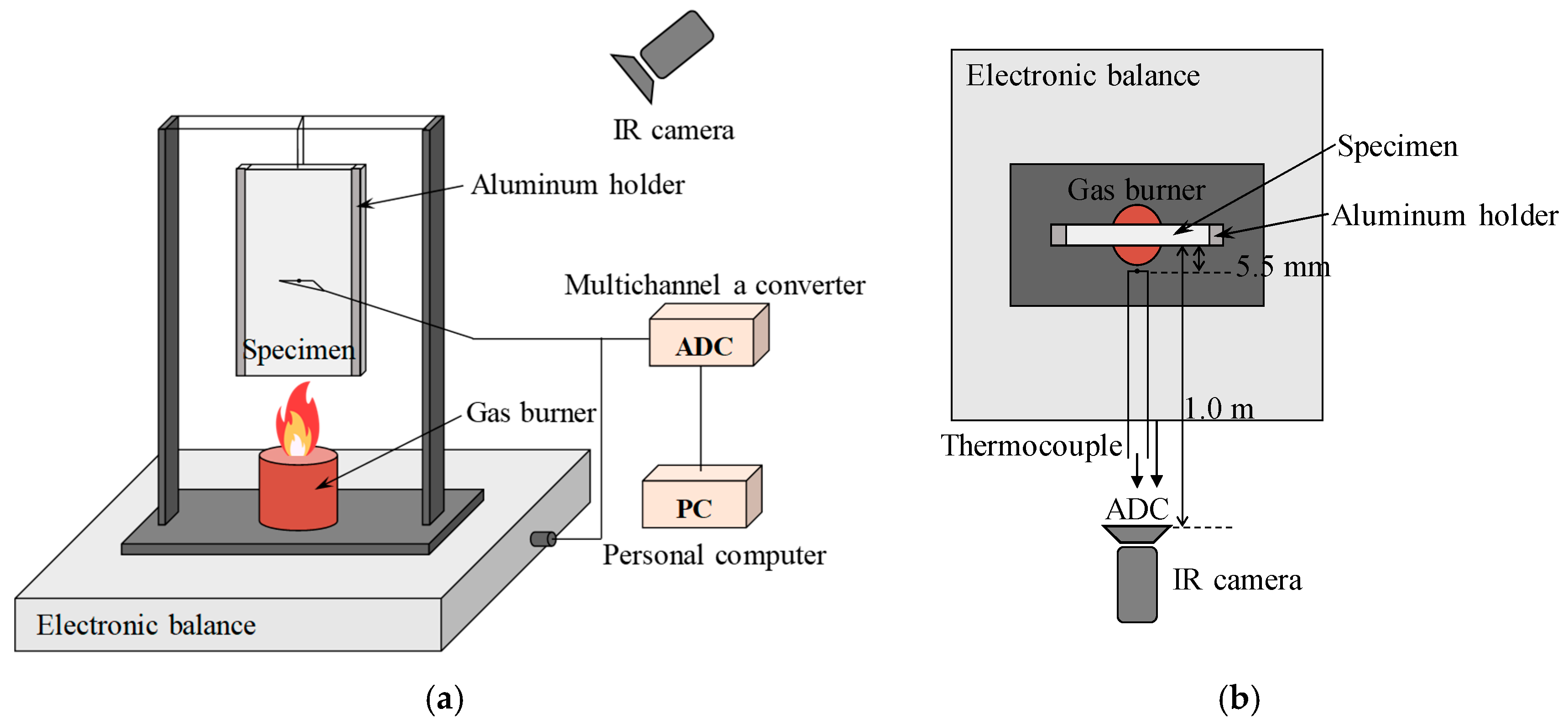
The vertical flame propagation experiment was conducted as illustrated in Figure 1 [13]. Specimens measuring 30 mm in width, 80 mm in length, and 1.2 mm in thickness were mounted above the nozzle tip of a Bunsen burner, and the upward flame propagation was observed. The prepreg slabs were fabricated using glass fiber fabric with a binder content of approximately 35.0%. The binder consisted of resin (ED-22), a curing accelerator (DYHARD UR5400), and a hardener (Dicyandiamide OKD 100S). The specimens were manufactured by vacuum molding and subjected to curing processes at 90 °C and 135 °C for 2 h each. On both sides of the specimens, aluminum holders covered with 5 mm-wide strips were attached, leaving an exposed specimen surface width of 20 mm.

The nozzle of the Bunsen burner was made of copper pipe with an internal diameter of 11 mm and a wall thickness of 1.5 mm. Through the nozzle, a laminar diffusion flame fueled by a propane–butane mixture was supplied, with the fuel flow rate set to 0.46 cm³/s. The gas temperature was measured using a Pt-(Pt + 10%Rh) thermocouple (wire diameter: 100 $\mathrm{\mu }\mathrm{m}$) at a position 5.5 mm away from the specimen surface, located 30 mm above the lower edge of the specimen. The mass variation in the specimen was also recorded. In addition, an infrared camera was installed 1 m away from the specimen to continuously monitor surface temperature.

3. Materials

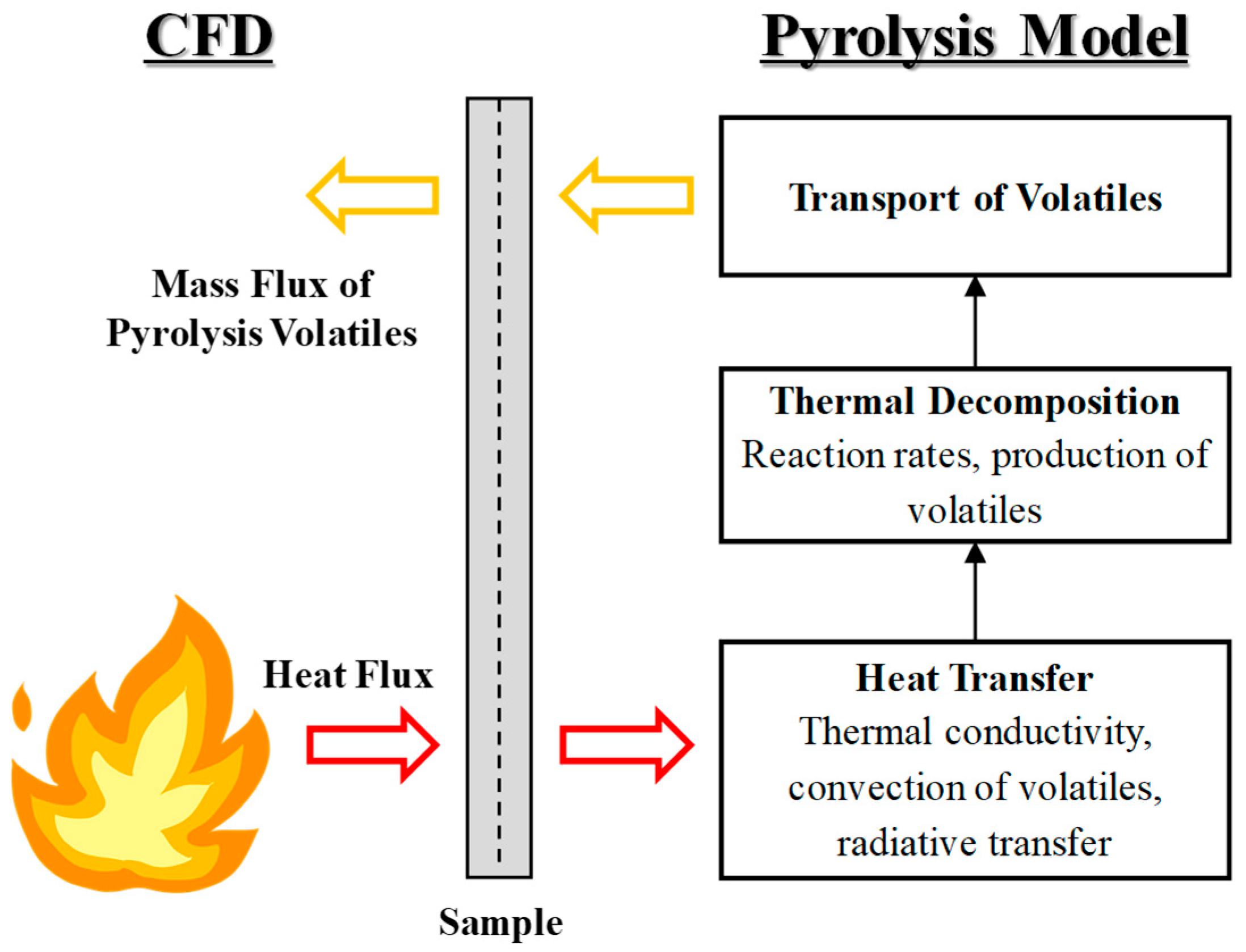
Computational Fluid Dynamics (CFD) is a numerical method for replicating and analyzing phenomena using physical and chemical models implemented in computer simulations. Among commercial CFD software packages, ANSYS Fluent 2023 R2 (version 23.2) is widely used, as it supports various physical models including heat transfer, combustion, turbulence, multiphase flow, and particle-laden flow. Through discretization techniques, it can generate results comparable to those from experiments or actual conditions, making it applicable across diverse industrial fields. However, due to inherent limitations of fluid dynamics, no direct predictive model exists for pyrolysis occurring in solid combustibles such as plastics or composite materials. To overcome this limitation, the present study employed User-Defined Functions (UDFs) within Fluent and introduced a pyrolysis model capable of numerically simulating the decomposition of composite materials, including the generation and release of volatiles. The interaction between the pyrolysis model and the CFD solver is illustrated in Figure 2.

When applying the pyrolysis model within CFD, thermal properties such as surface temperature and heat flux are used as input parameters to calculate the mass flow rate of volatiles generated through pyrolysis. This value is then expressed as the mass flux at the specimen surface. To compute the mass flux originating from the solid phase, the following assumptions were made:

• The specimen undergoing pyrolysis is assumed to have a sandwich structure, with pyrolysis occurring on both surfaces.
• At the beginning of the analysis, the solid phase is considered homogeneous, composed of fiber and matrix polymer.
• An irreversible pyrolysis reaction occurs in the matrix polymer, producing volatile compounds and char. A single-step reaction is considered in this study.
• The pyrolysis reaction is modeled using the conversion function ($f\left(\alpha \right)$), apparent activation energy ($E_a$), pre-exponential factors ($A$).
• In the three-dimensional CFD analysis, the spatial distribution of the specimen surface is represented in two dimensions, and each cell on the surface is treated independently.
• Both the solid and gas phases are assumed to be in local thermal equilibrium.
• Changes in thickness and geometry of the specimen due to pyrolysis are not considered in the CFD analysis.

3.1. Flame Propagation Model

3.1.1. Kinetics of Thermal Decomposition

The kinetic characteristics of material pyrolysis can be derived using Microscale Combustion Calorimetry (MCC), and the model simulating the MCC measurements is expressed in the form of Equations (1) and (2).

$${\displaystyle \frac{dT}{dt}}=\beta , T\left(0\right)=T_0$$

(1)

$$\dot{q}=\overline{∆q^{\prime }}{\displaystyle \frac{d\alpha }{dt}}=\overline{∆q^{\prime }}Af\left(\alpha \right)\exp \left(-{\displaystyle \frac{E_a}{RT}}\right), \alpha \left(0\right)=0$$

(2)

Here, $T$ denotes the temperature of the specimen, $\beta$ the heating rate, $\overline{∆q^{\prime }}$ the heat of combustion of volatiles per unit mass of the initial material, $\alpha$ the heat-release-based conversion (defined as the ratio of the current heat release rate to ($\overline{∆q^{\prime }}$), R the universal gas constant, $f\left(\alpha \right)$ the conversion function, $E_a$ the apparent activation energy, and $A$ the pre-exponential factor. The conversion function $f\left(\alpha \right)$ was estimated from experimental results and can be expressed as $\left({\alpha }^m+{\alpha }^{*}\right){\left(1-\alpha \right)}^n$, with the values of each parameter summarized in

Table 1. Kinetic parameters of the decomposition reaction [13].

No.	Variable	Content	Value
1	$R$	Universal gas constant	(8.314 J/mol$·$K)
2	$E_a$	Apparent activation energy	136.9 kJ/mol
3	$A$	Pre-exponential factors	8.555$·$108/s
4	$m$	-	0.18
5	$n$	-	1.5
6	${\alpha }^{*}$	-	0.001

.

From the MCC tests, the heat of combustion of volatiles was measured to be 25.4 ± 0.2 kJ/g, and the mass fraction of the solid residue $Y_{res}$ at the final stage was determined to be 0.658.

To apply the pyrolysis model, the volume fraction of fiber $X_{fib}$ and the mass fraction of polymer converted into volatiles $v_g$ are defined. These two variables can be obtained from the residue mass fraction $Y_{res}$ using Equations (3) and (4).

$$Y_{res}={\displaystyle \frac{m_{\infty }}{m_0}}={\displaystyle \frac{m_{fib}+m_{ch}}{m_{fib}+m_{mp,0}}}={\displaystyle \frac{X_{fib}{\rho }_{fib}+\left(1-v_g\right)\left(1-X_{fib}\right){\rho }_{mp}}{\rho }}$$

(3)

$$\rho =X_{fib}{\rho }_{fib}+\left(1-X_{fib}\right){\rho }_{mp}$$

(4)

In Equation (3), $\rho$ represents the initial density of the specimen, $m_0$ is the initial mass of the fiber and polymer (measured as 2.63 g), and $m_{\infty }$ is the residual mass of the specimen after completion of the combustion reaction (measured as 1.73 g). The density $\rho$ was determined to be 1370 kg/m³, and the material properties of the other components are listed in

Table 2. Thermal properties of the components [13].

	Thermal Conductivity (W/m$·$K)	Density (kg/m3)	Specific Heat (J/kg$·$K)
Polymer ($\mathit{mp}$)	0.28	1250	800
Fiber ($\mathit{fib}$)	0.28	1750	800
Char ($\mathit{ch}$)	30.0	1800	1720

. From the calculation of Equation (4), $X_{fib}$ is obtained as 0.24, and using Equations (3) and (4), $v_g$ is calculated to be 0.494, as shown in Equation (5).

$$v_g=1-{\displaystyle \frac{Y_{res}\rho -X_{fib}{\rho }_{fib}}{\left(1-X_{fib}\right){\rho }_{mp}}}$$

(5)

3.1.2. Calculating Heat Transfer Using Equations Conservation of Energy and Mass

The constituents of the composite material are represented by three components: the original composite matrix ($fib$) prior to flame exposure, the polymer decomposed by the flame ($mp$), and the residual char ($ch$). When dividing the specimen into solid and gaseous phases, the volume fractions of gas ($X_g$) and solid ($X_s$) satisfy the relation $X_g+X_s=1$. For the solid phase, the three mass fractions corresponding to each constituent—$X_{s,fib}$, $X_{s,mp}$, and $X_{s,ch}$—satisfy the relation $X_{s,fib}$ + $X_{s,mp}$+ $X_{s,ch}$ = 1. In the pyrolysis model, the conservation of mass between the gaseous and solid phases during pyrolysis is described by Equations (6) and (7).

$${\displaystyle \frac{\mathit{\partial }{\left(1-\varnothing \right)}_{{\rho }_s}}{\mathit{\partial }t}}=-{g^{″}}^{\prime }$$

(6)

$${\displaystyle \frac{\mathit{\partial }\varnothing {\rho }_s}{\mathit{\partial }t}}+{\displaystyle \frac{\mathit{\partial }{g}^{″}}{\mathit{\partial }x}}=-{g^{″}}^{\prime }$$

(7)

In Equations (6) and (7), ${g^{″}}^{\prime }$ represents the mass generation rate of gaseous volatiles due to pyrolysis (kg/m³·s), and $g^{″}$ denotes the mass flux in the gas phase (kg/m²·s). The conservation of energy is then expressed by Equations (8) and (9).

$${\displaystyle \frac{\mathit{\partial }\left(1-\varnothing \right){\rho }_s{h}_s}{\mathit{\partial }t}}+{\displaystyle \frac{\mathit{\partial }}{{\mathit{\partial }}_x}}{q^{″}}_{cond,s}=-{{q^{″}}^{\prime }}_r$$

(8)

$${\displaystyle \frac{\mathit{\partial }\varnothing {\rho }_s{h}_s}{\mathit{\partial }t}}+{\displaystyle \frac{\mathit{\partial }}{{\mathit{\partial }}_x}}\left(q^{″}{h}_g+{q^{″}}_{cond,s}\right)=0$$

(9)

$h_s$ and $h_g$ represent the enthalpy of the solid and gas phases, respectively, and are expressed in Equations (10) and (11).

$$h_s=h_s^0+{{\displaystyle \int }}_{T^0}^T{c}_s\left(T\right)dT$$

(10)

$$h_g=h_g^0+{{\displaystyle \int }}_{T^0}^T{c}_g\left(T\right)dT$$

(11)

In Equations (10) and (11), $c_s$ and $c_g$ denote the specific heat of the solid and gas phases, respectively; $h_s^0$ and $h_g^0$ represent the reference enthalpies of each phase at the reference temperature $T^0$ ${q^{″}}_s$ and ${q^{″}}_g$ correspond to the conductive heat fluxes; and ${{q^{″}}^{\prime }}_r$ represents the radiative heat term. Assuming thermal equilibrium between the solid and gas phases such that their temperatures are identical, Equations (8) and (9) can be combined into a single energy conservation equation, expressed as Equation (12).

$${\displaystyle \frac{\mathit{\partial }}{\mathit{\partial }t}}\left(\varnothing {\rho }_s{h}_s+\left(1-\varnothing \right){\rho }_s{h}_s\right)+{\displaystyle \frac{\mathit{\partial }}{{\mathit{\partial }}_x}}\left(q^{″}{h}_g+{q^{″}}_{cond,s}\right)=-{{q^{″}}^{\prime }}_r$$

(12)

In Equation (9), ${q^{″}}_{cond}=-k{\displaystyle \frac{\mathit{\partial }T}{\mathit{\partial }x}}$ represents the conductive heat flux in the porous medium where the solid and gas phases coexist, while ${{q_r}^{\prime \prime }}^{\prime }={\displaystyle \frac{\mathit{\partial }{q_r}^{\prime \prime }}{\mathit{\partial }x}}$ denotes the radiative heat flux emitted from the specimen surface. The thermal conductivity $k$ is expressed as a weighted sum of the conductivities of the solid and gas phases, where both phases are assumed to consist of components parallel ($k_{\parallel }$) and perpendicular ($k_{\perp }$) to the specimen surface.

$$k=k_{\parallel }WF+k_{\perp }\left(1-WF\right)=\left(\varnothing k_g\left(1-\varnothing \right)k_s\right)WF+{\left({\displaystyle \frac{\varnothing }{k_g}}+{\displaystyle \frac{1-\varnothing }{k_s}}\right)}^{-1}\left(1-WF\right)$$

(13)

In Equation (13), $k_s$ can be expressed as $k_{s,i}$ according to the proportion of each constituent component of the solid phase.

$$k=k_{\parallel }WF+k_{\perp }\left(1-WF\right)=\left({\displaystyle \sum }_i{X}_{s,i}{k}_{s,i}\left(T\right)\right)WF+{\left({\displaystyle \sum }_i{\displaystyle \frac{X_{s,i}}{k_{s,i}\left(T\right)}}\right)}^{-1}\left(1-WF\right)$$

(14)

At elevated temperatures, such as those encountered during combustion, radiative heat transfer within pores becomes significant. In this study, the radiative conductivity $k_g$ was incorporated, and the radiation correction term $k_{g,r}=k_g\left(T\right)+{\delta }_r\left(16/3\right)\sigma T^3$ was substituted into $k_g$ in Equation (13). By substituting the mass conservation equations (Equations (6) and (7)) together with the relations in Equations (10) and (11) into the energy equation (Equation (12)), the formulation can be rearranged as shown in Equation (15).

$$\rho c{\displaystyle \frac{\mathit{\partial }T}{\mathit{\partial }t}}+g^{″}{c}_g{\displaystyle \frac{\mathit{\partial }T}{\mathit{\partial }x}}-{\displaystyle \frac{\mathit{\partial }}{\mathit{\partial }x}}k{\displaystyle \frac{\mathit{\partial }T}{\mathit{\partial }x}}={{q^{″}}^{\prime }}_g+{{q^{″}}^{\prime }}_r$$

(15)

In Equation (15), $\rho c=\varnothing {\rho }_g{c}_g+\left(1-\varnothing \right){\rho }_s{c}_s$, and ${{q^{″}}^{\prime }}_g=\left(h_s-h_g\right){q^{″}}^{\prime }=∆h_g{q^{″}}^{\prime }$. Each specimen surface is influenced by the radiative heat flux ${q^{″}}_r$ and the convective heat flux ${q^{″}}_c$ from the adjacent gas phase. The net heat flux, expressed as the sum of these contributions, is given as ${q^{″}}_{net}$ in Equation (16).

$${q^{″}}_{net}={q^{″}}_r+{q^{″}}_c$$

(16)

The radiative heat flux is given by the product of the absorptivity and the incident radiative flux, minus the re-radiated flux from the surface.

$${q^{″}}_r=ϵq_{r,inc}\prime \prime -ϵ\sigma T_{surf}^4$$

(17)

3.1.3. Computation of Radiative Heat Transfer in Flame Propagation Models

Radiative heat transfer is modeled by dividing the specimen into the right side ($x_{right}$) and the left side ($x_{left}$). The incident radiation $G$ and the radiative heat flux ${q^{″}}_r$ are expressed in Equations (18) and (19), respectively.

$${\displaystyle \frac{1}{k_s}}{\displaystyle \frac{d{q^{″}}_r}{dx}}=4\mathsf{\sigma }{T}^4-G$$

(18)

$${q^{″}}_r=-{\displaystyle \frac{1}{4k_s}}{\displaystyle \frac{dG}{dx}}$$

(19)

Here, $k_s$ denotes the absorption coefficient. By substituting Equation (19) into Equation (18), a second-order differential equation for the incident radiation can be obtained.

$${\displaystyle \frac{1}{4k_s}}{\displaystyle \frac{d}{dx}}\left({\displaystyle \frac{1}{k_s}}{\displaystyle \frac{dG}{dx}}\right)=G-4\mathsf{\sigma }{T}^4$$

(20)

For Equation (20), the boundary conditions are defined by applying the emissivities ${ϵ}^{\left(1\right)}$ and ${ϵ}^{\left(2\right)}$, which allow for the absorption and emission of radiative heat.

$$x_{left}: {\displaystyle \frac{1}{4k_s}}{\displaystyle \frac{dG}{dx}}={\displaystyle \frac{2{ϵ}^{\left(1\right)}}{2-{ϵ}^{\left(1\right)}}}\left(-{\displaystyle \frac{G}{4}}+\mathsf{\sigma }{T}^4\right)$$

(21)

$$x_{right}: {\displaystyle \frac{1}{4k_s}}{\displaystyle \frac{dG}{dx}}={\displaystyle \frac{2{ϵ}^{\left(2\right)}}{2-{ϵ}^{\left(2\right)}}}\left({\displaystyle \frac{G}{4}}+\mathsf{\sigma }{T}^4\right)$$

(22)

By solving Equation (20) together with the boundary conditions given in Equations (21) and (22), the emissive power of the radiative heat flux can be determined.

$${\displaystyle \frac{\mathit{\partial }{q^{″}}_r}{\mathit{\partial }x}}=k_s\left(4\mathsf{\sigma }{T}^4-G\right)$$

(23)

Equation (23) is used as a source term in the energy conservation equation.

3.1.4. Chemical Reactions and the Formation of Volatile Compounds

In this study, a single-step pyrolysis reaction was considered. The chemical reaction can be expressed as shown in Equation (24).

$$m_{mp}\to \left(1-v_g\right)m_{mp}+v_g{m}_{mp}$$

(24)

$$\dot{r}={\displaystyle \frac{d\alpha }{dt}}=-{\displaystyle \frac{1}{m_{mp,0}-m_{mp,\infty }}}{\displaystyle \frac{d{m}_{mp}}{dt}}={\displaystyle \frac{1}{v_g{m}_{mp}}}{\displaystyle \frac{d{m}_{mp}}{dt}}$$

(25)

In Equation (25), $m_{mp}$ denotes the mass of the polymer (kg/m²) within each grid cell, which varies over time due to combustion.

$$\mathsf{\alpha }={\displaystyle \frac{m_{mp,0}-m_{mp}}{m_{mp,0}-m_{mp,\infty }}}={\displaystyle \frac{1}{v_g}}\left(1-{\displaystyle \frac{m_{mp}}{m_{mp,0}}}\right)$$

(26)

The conversion variable $\alpha$ represents the progress of the chemical reaction and takes values between 0 and 1. The reaction rate is determined as follows.

$$\dot{r}=Af\left(\alpha \right)\exp \left({\displaystyle \frac{E_a}{RT}}\right)$$

(27)

Equation (27) can be rearranged into the form of Equation (28).

$${\displaystyle \frac{d{m}_{mp}}{dt}}=-v_g{m}_{mp,0}\dot{r}=-\dot{R}$$

(28)

By discretizing Equation (28) over a small-time interval ($∆t$), it can be expressed as shown in Equation (29).

$${\displaystyle \frac{m_{mp}^{n+1}-m_{mp}^n}{∆t}}={\displaystyle \frac{\frac{m_{mp}^n+m_{mp}^{n+1}}{2}}{m_{mp}^n}}min\left(\dot{R},2{\displaystyle \frac{m_{mp}^n}{∆t}}\right)$$

(29)

Rearranging for $m_{mp}^{n+1}$, the formulation can be expressed as Equation (30).

$$m_{mp}^{n+1}=m_{mp}^n\max \left({\displaystyle \frac{m_{mp}^n-\dot{R}∆t/2}{m_{mp}^n+\frac{\dot{R}∆t}{2}}},0\right)$$

(30)

To prevent $m_{mp}^{n+1}$ from taking negative values, a max function was applied as a constraint. The amount of volatile matter generated at each time step is expressed as ${q^{″}}^{\prime }=\left(v_g\left(m_{mp}^{n+1}-m_{mp}^n\right)/∆t\right)/∆x$, where $∆x$ denotes the area of the grid cell.

3.2. Numerical Simulation Strategies and Boundary Conditions

3.2.1. Geometric Model, Grids, and Time Steps

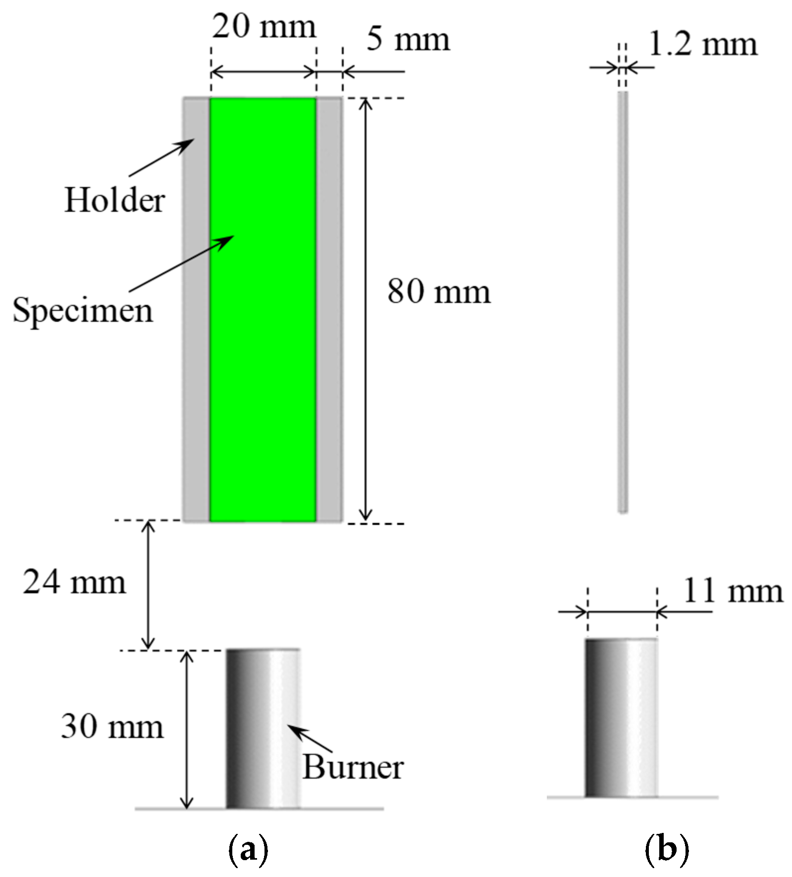
The entire computational domain was defined as a cylinder with a diameter of 0.3 m and a height of 0.32 m. As shown in Figure 3, the analysis model included a tube-shaped burner with a diameter of 11 mm, a thickness of 1.2 mm, and a height of 30 mm installed at the bottom surface. The specimen was positioned at the center, 24 mm above the top of the burner. The specimen dimensions were 80 mm in length, 20 mm in width, and 1.2 mm in thickness, with aluminum holders of 5 mm in width attached on both sides, having the same thickness and length as the specimen.

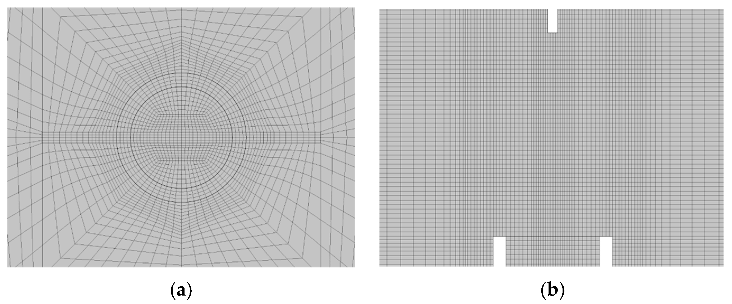
As illustrated in Figure 4, the computational grid consisted of approximately 1,370,000 hexahedral cells. In the previous research, similar results were obtained with a coarse mesh (388,752 elements), which is about a quarter of the fine mesh (1,513,472 elements) [13]. In this study, 0.3 mm mesh was generated near the specimen surface and applied a bias factor to the space above the specimen, reducing the number of mesh. To ensure the stability of the initial combustion analysis, the region up to 25 mm above the burner outlet was filled with 100% propane mass fraction. The subsequent 5 mm-high region above the burner tip was initialized with a temperature of 1200 K and reaction products corresponding to complete combustion. The time step size was set to 0.001 s, and the simulation was performed for a total duration of 80 s.

3.2.2. Setting Conditions

In this analysis, laminar flow was assumed due to the low inlet velocity of the burner. To separately calculate the chemical reactions occurring in the lower burner and the volatiles released from the specimen surface, the burner reactant was assumed to be propane (C₃H₈), while the volatiles from the specimen were assumed to be ethylene (C₂H₄) with a heat of combustion of 25.4 kJ/g, as measured in experiments. Although volatile transport in porous media typically follows Darcy’s law, porous effects were not considered in this analysis, and therefore mass transport within porous media was not included. The fuel mass flow rate at the burner inlet was set to 0.88 mg/s with an inlet temperature of 300 K. The chemical reaction for propane was defined as C₃H₈ + 5O₂→3CO₂ + 2H₂O, with an activation energy of 125.6 kJ/mol, a pre-exponential factor of 4.836 × 10⁹, and reaction orders of 0.1 for hydrocarbons and 1.65 for oxygen. The reaction for ethylene was defined as C₂H₄ + 3O₂→2CO₂ + 2H₂O, with an activation energy of 121 kJ/mol, a pre-exponential factor of 7.516 × 10¹², and reaction orders of 0.42 for hydrocarbons and 1.27 for oxygen.

For simulating chemical reactions, the species transport model was employed, and the stiff chemistry solver with the In Situ Adaptive Tabulation (ISAT) method was used to improve computational efficiency. The DO model was applied to account for radiative heat transfer.

3.3. Validation with Experimental Results

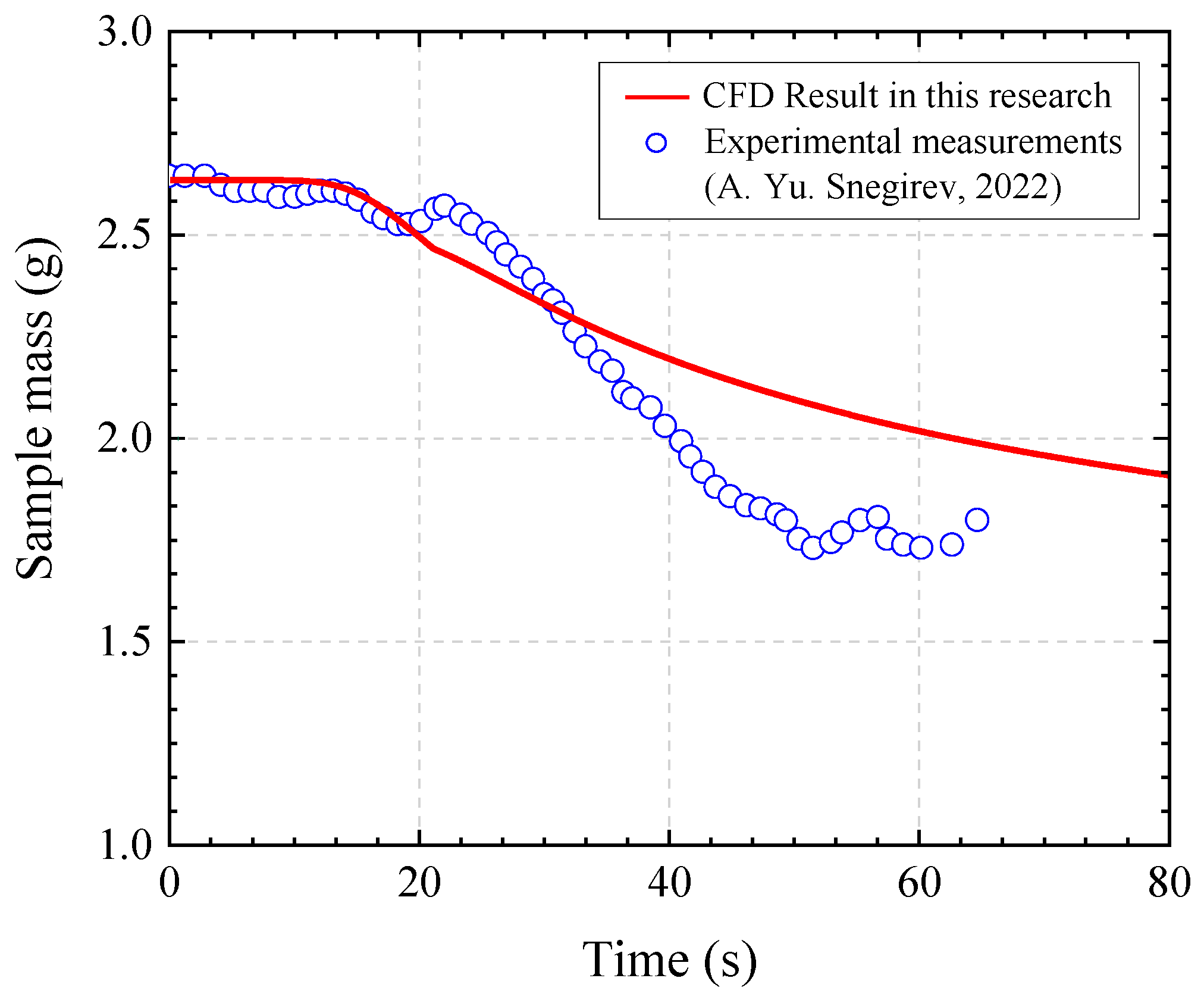
To compare the CFD analysis results of this study with experimental findings from previous literature [13], Figure 5 presents the mass loss of the specimen as a function of time. The analysis showed that from the initial calculation time (0 s) to approximately 30 s, the mass variation in the specimen was consistent with experimental observations. However, beyond this point, the residual mass predicted by the present analysis was observed to be higher. This discrepancy is attributed to differences in grid resolution and to the exclusion of volatile transport within porous media in the simulation conditions. Nevertheless, since the mass variation during the early stage—immediately after ignition, when flame propagation begins—was in good agreement with previous studies, it is concluded that the proposed model can physically and reliably predict the pyrolysis and flame propagation behavior of non-porous solid materials. 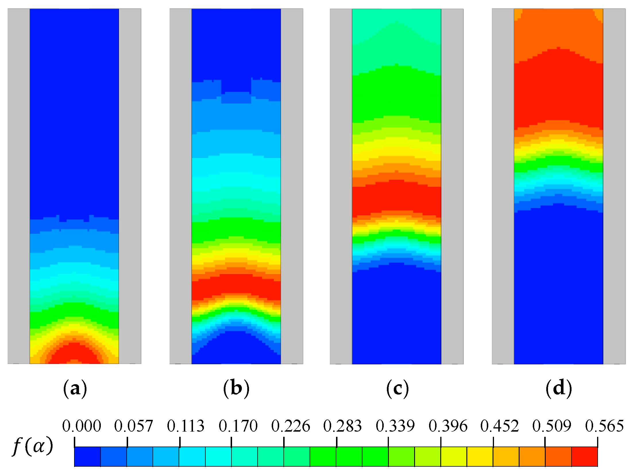Figure 6 illustrates the temporal evolution of the conversion function $f\left(\alpha \right)$ on the specimen surface. The function $f\left(\alpha \right)$ represents the region where pyrolysis reactions predominantly occur, and it was observed that the reaction zone rose over time as the flame propagated.

4. Ultra-Fast Fire Analysis in Industrial Complexes

Unlike ordinary fires, those occurring in industrial complex facilities may develop into ultra-fast fires, in which the heat release rate increases sharply over time, resulting in a rapid intensification of fire severity. Such events can reach a heat release rate of approximately 1 MW within just one minute, causing significant damage to medium-sized factories and similar facilities. However, ultra-fast fires are currently described only in terms of their heat release rate curves, with no clear definitions or application boundaries, highlighting the need for further studies to characterize their behavior.

In this study, the previously validated pyrolysis model, capable of analyzing ultra-fast fire behavior, was applied to industrial complex facilities with a floor area of less than 1000 m². The first analysis applied fire growth scenarios—derived from fire growth rates and the time to reach peak heat release—into the computational model, and CFD simulations were performed to numerically analyze the temperature and flame distribution during fire development. The second analysis extended the validated model to a full-scale industrial facility, where flame propagation patterns under different fire scenarios were investigated.

4.1. Modeling and Simulations

4.1.1. Simulations for Fire Growth Scenarios

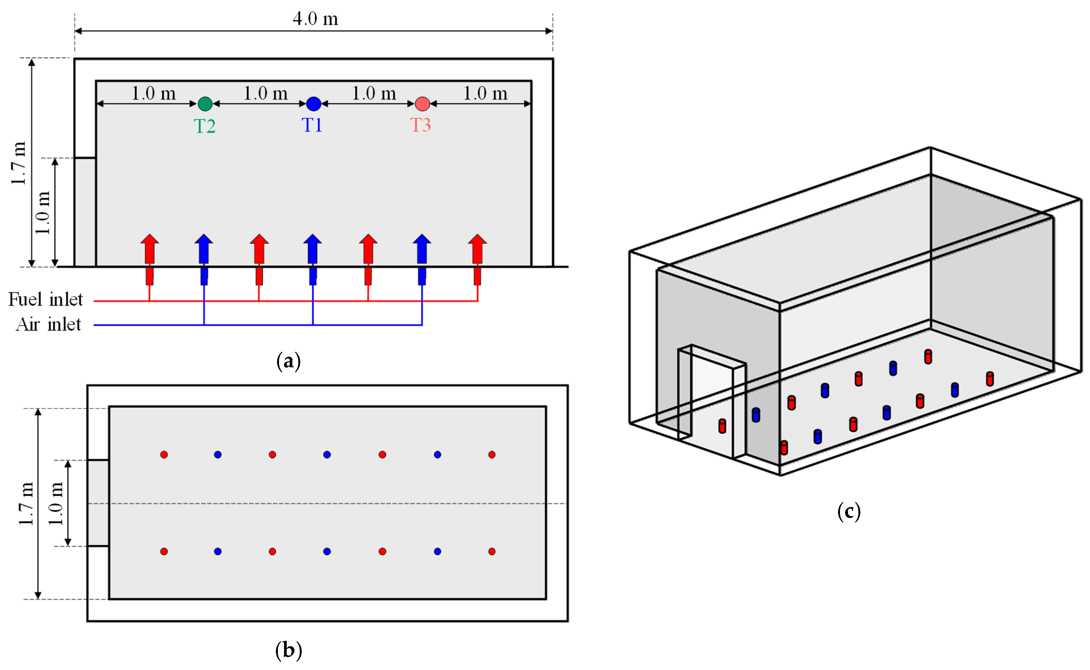
For the numerical analysis, a model structure with dimensions of 4.0 m in length, 1.8 m in width, and 1.7 m in height was constructed based on a realistic scale, as illustrated in Figure 7. If the fire occurring inside the compartment were to be assumed as a closed system, it would be difficult to accurately simulate combustion reactions and heat release because they strongly depend on the ratio of fuel to oxidizer. Therefore, an opening measuring 1 m in both width and height was created at the center of the model, while oxygen and fuel (methane) were supplied from the floor to establish combustion conditions.

Prior to applying the fire growth scenario, a preliminary numerical simulation was conducted under the condition of a constant heat release rate of 1 MW to examine the temperature rise trend within the upper region of the model compartment. In this analysis, a single-step reaction mechanism (CH₄ + 2O₂→CO₂ + 2H₂O) was applied, in which methane (CH₄) and oxygen (O₂) react to produce carbon dioxide (CO₂) and water (H₂O). Based on the enthalpy of formation of the combustion products CO₂ and H₂O (−877,236 kJ/k·mol), the methane mass inflow rate was set to 0.01828 kg/s. The volumetric flow rate of air was calculated as twice the molar quantity of the fuel and was applied as the velocity boundary condition.

Following this preliminary analysis, an additional simulation was performed by applying a fire growth curve with a growth coefficient of $\mathsf{\alpha }$ = 1.876, in which the heat release rate increased over time and reached 100 MW at 12 min and 15 s. The fuel inflow was determined using the same method as in the initial case, while the inlet flow rates of fuel and oxidizer were defined as time-dependent functions using the Expression feature of ANSYS Fluent.

4.1.2. Simulations of Flame Propagation in Full-Scale Enclosures

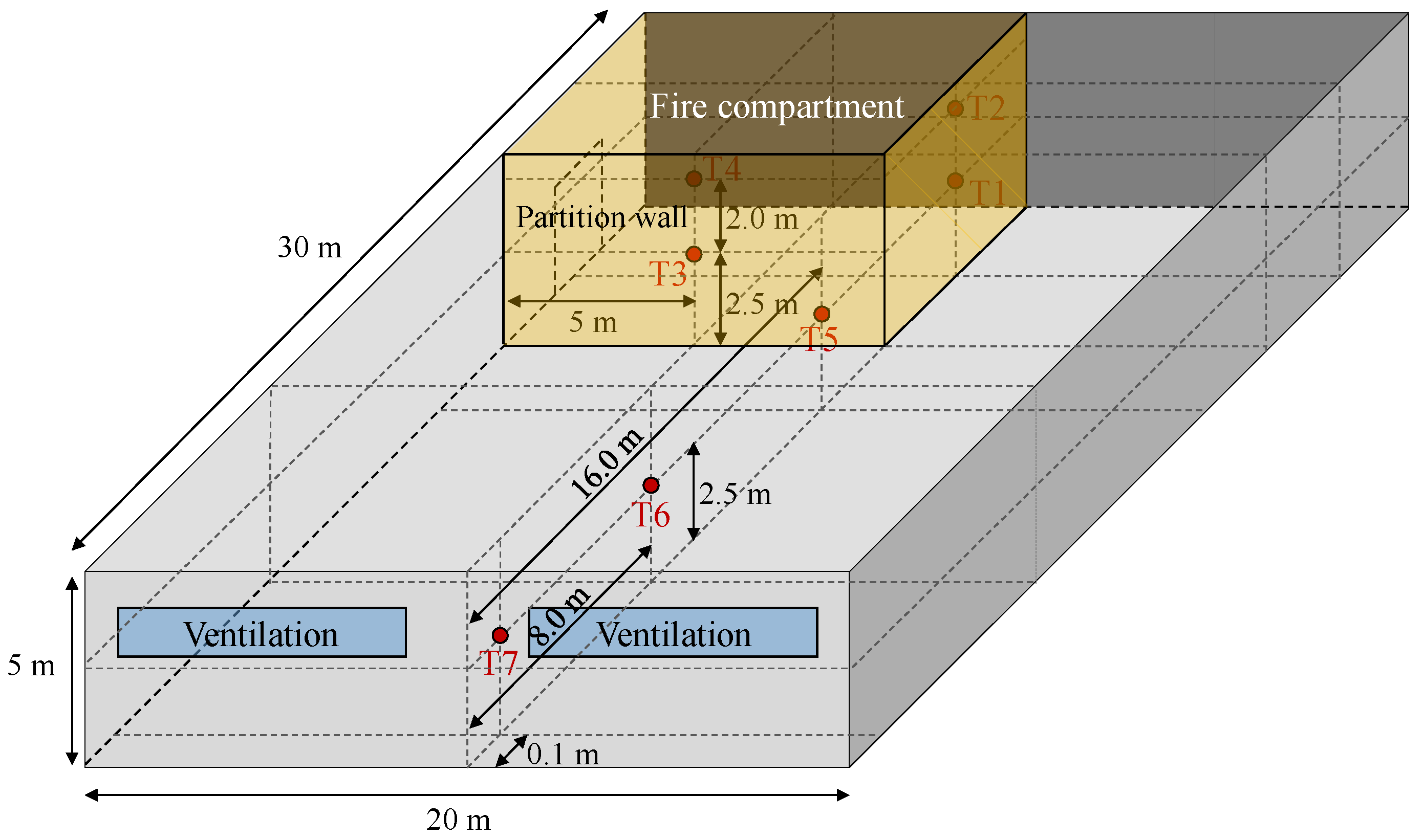
For the numerical analysis of industrial complex facilities, a full-scale model structure measuring 20.0 m in length, 30.0 m in width, and 5.0 m in height was developed, as illustrated in Figure 8. To ensure similarity with realistic conditions, the initial fire region was set to 5.0 m in length and 10.0 m in width. As shown in Figure 8, the simulation assumed a fire scenario in which combustion occurred within a compartmented space during the first minute after ignition, followed by the opening of the partition wall, allowing the fire to spread throughout the entire domain over a period of 12 min.

The fire growth conditions were set identical to those in Section 4.1.1 Simulations for Fire Growth Scenarios, with fuel and oxidizer inlets evenly distributed along the bottom of the model. Temperature data were collected over time at a total of seven locations: four points (T1–T4) within the fire origin zone and three points (T5–T7) in the external region. In addition, to simulate pyrolysis of the wall surfaces and the subsequent flame propagation behavior, a User-Defined Function (UDF) in ANSYS Fluent was applied. Through the UDF, fuel release was triggered once the wall temperature reached a critical threshold, and the fuel release rate was modeled as a time-dependent function. To simulate flame propagation from an initial ignition source, a temperature of 1500 K was applied as an initial condition to a cell with an area of 0.1 × 0.1 m at the corner of the fire compartment. This approach enabled a more realistic representation of flame propagation spreading outward from the ignition source.

4.2. Results and Discussions

4.2.1. Simulations Results for Fire Growth Scenarios

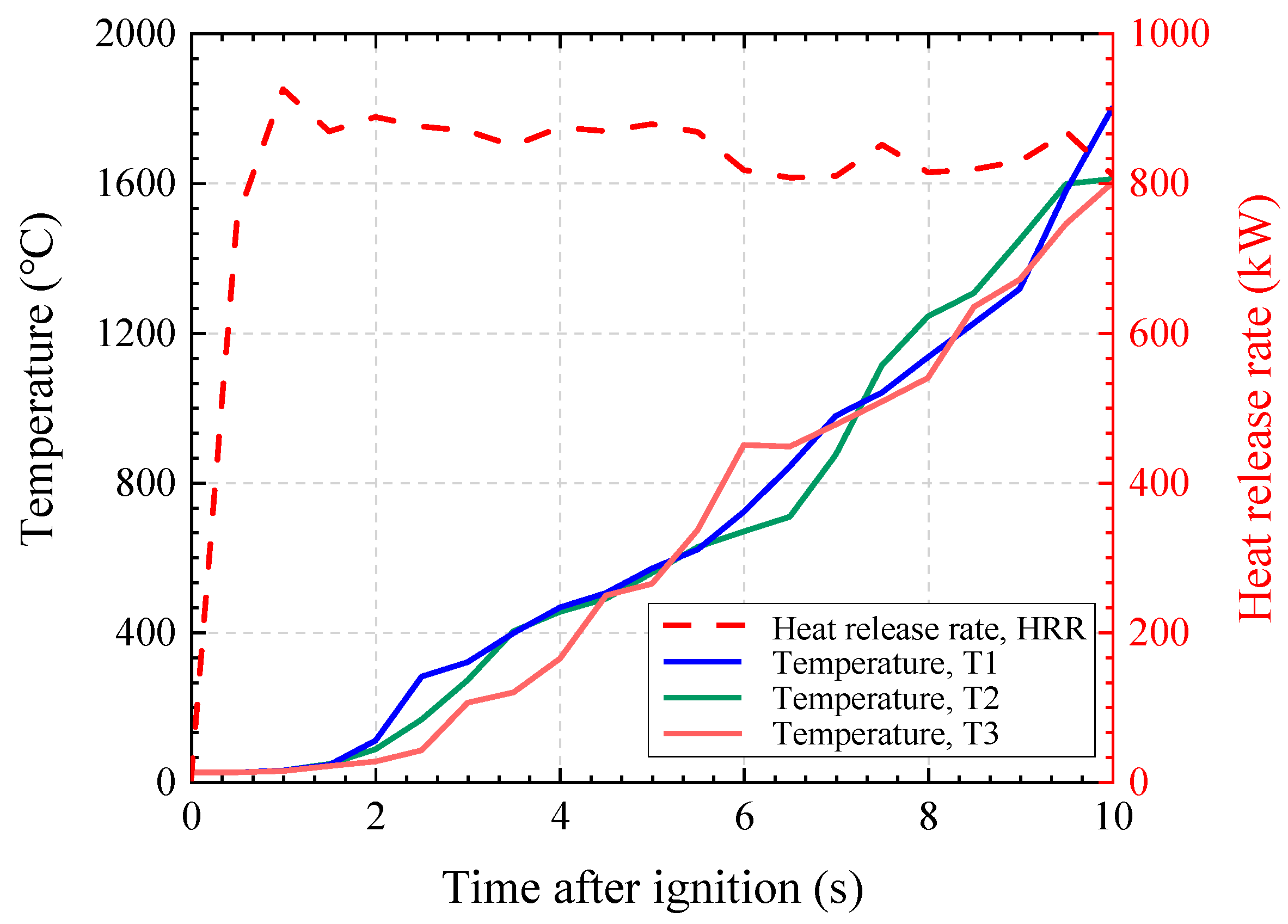
A CFD analysis was conducted under the assumption of a constant heat release rate of 1 MW. The total simulation time was set to 10 s, and the temporal variations in temperature and heat release rate (HRR) at three locations (T1–T3) inside the model are presented in Figure 9. HRR means summation of the volumetric heat of reaction within the computational domain. In ANSYS Fluent, volumetric heat of reaction in each cell is computed as follows: $S_h=-{{\displaystyle \sum }}_j{\displaystyle \frac{h_j^0}{M_j}}{R}_j$. Where $h_j^0$ is the enthalpy of formation, $M_j$ is the molecular weight, and $R_j$ is the volumetric rate of creation of species $j$. Although the methane inflow corresponding to a theoretical HRR of 1 MW was specified as a boundary condition, the actual simulation results showed HRR values of approximately 900–800 kW over time. This discrepancy is attributed to the characteristics of the combustion modeling process, in which part of the fuel escaped through internal boundaries before complete combustion could occur.

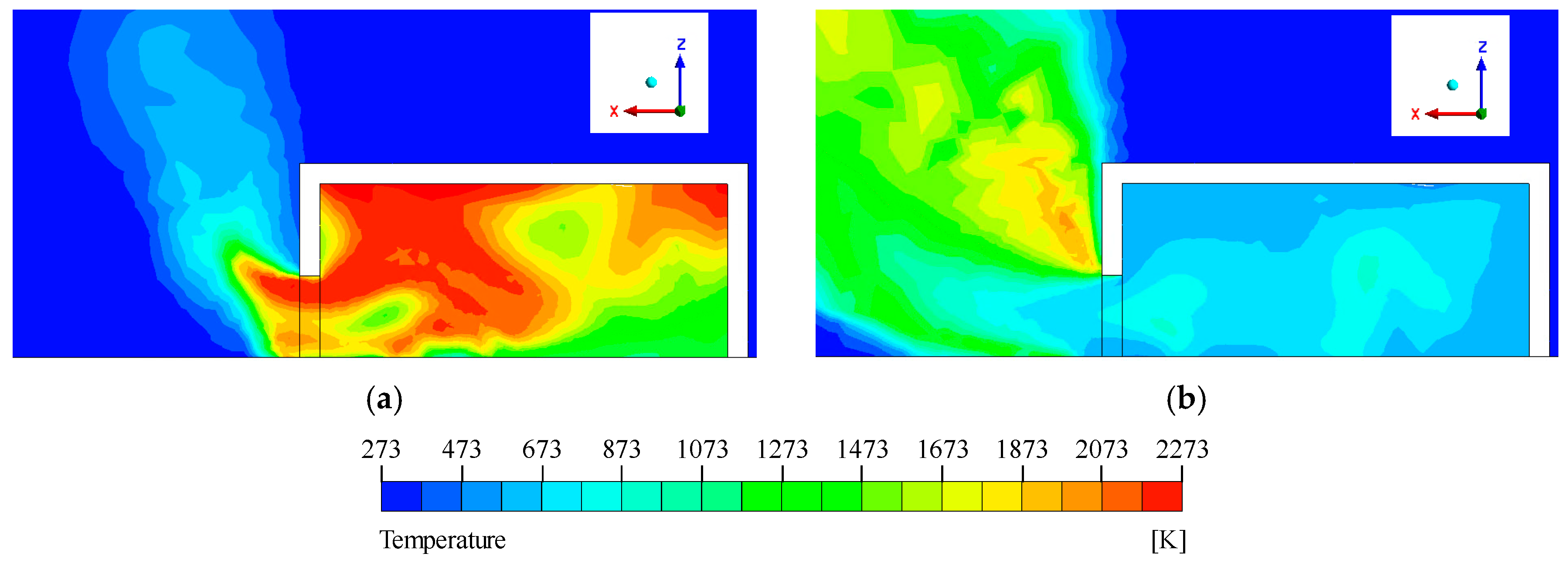
The temperature exhibited a continuous upward trend over time, converging to approximately 1600–1800 °C at the end of the 10 s simulation. Since all three measurement points were located at the same height, the temporal variation in temperature appeared similar across these locations. Meanwhile, as shown in Figure 10, the temperature distribution at the end of the simulation revealed a localized high-temperature region near the innermost upper wall, due to the structural characteristic of having no outlet. At this location, the maximum temperature was found to reach approximately 2073 °C.

Subsequently, under the same conditions, a fire growth curve with a growth coefficient of $\mathsf{\alpha }$ = 1.876 was applied, and a CFD simulation was conducted in which the heat release rate (HRR) increased over time, reaching 100 MW at 12 min and 15 s. The simulation was performed for 500 s, and the HRR values and temperature distributions at different locations are presented in Figure 11. As shown in Figure 11a, the HRR within the internal region of the model remained relatively stable over time, whereas the external region exhibited a continuous increase. Furthermore, as shown in Figure 11b, the temperatures measured at three internal points were maintained at approximately 2000 °C until about 200 s after ignition, after which they gradually decreased, reaching around 500 °C at the end of the simulation (500 s). This trend is further illustrated in Figure 12. At 100 s (Figure 12a), the central cross-section of the model showed a high-temperature zone of about 2000 °C, resulting from the combustion reactions inside the compartment. In contrast, at 500 s (Figure 12b), the same cross-section showed a significantly reduced internal temperature of around 500 °C, while relatively higher temperatures of approximately 1000–1200 °C were observed near the outlet region. These results indicate that, unlike the constant 1 MW initial condition, the increasing HRR scenario led to substantially higher inflow rates of fuel and oxidizer. Consequently, incomplete combustion occurred inside the compartment, allowing excess fuel to escape and combust in the external region, thereby increasing the HRR outside. In addition, due to the higher inflow velocity of fuel and oxidizer, combustion reactions occurred predominantly near the outlet rather than inside, which explains the high temperatures observed in the outlet region in Figure 12b.

4.2.2. Simulations Results of Flame Propagation in Full-Scale Enclosures

For the full-scale model, the CFD analysis was conducted under the condition that the partition wall remained closed during the first 1 min, after which it was opened for the subsequent 12 min. The temporal variations in HRR and the temperature distributions at different locations are presented in Figure 13. As shown in Figure 13a, the computed HRR values were slightly higher than the prescribed input curve; however, the overall increasing trend was consistent and closely followed the fire growth curve. In addition, Figure 13b shows that the temperatures at locations T1–T4, situated within the compartment, increased up to 60 s before the partition wall was opened, then temporarily decreased, and subsequently increased again. Meanwhile, locations T1, T3, T5, T6, and T7—being at the same height—exhibited similar temperature distributions. This phenomenon is attributed to the fact that the data were obtained at the same vertical level, where the flow was not yet fully developed, and thus buoyancy-driven effects led to comparable thermal behavior across those points.

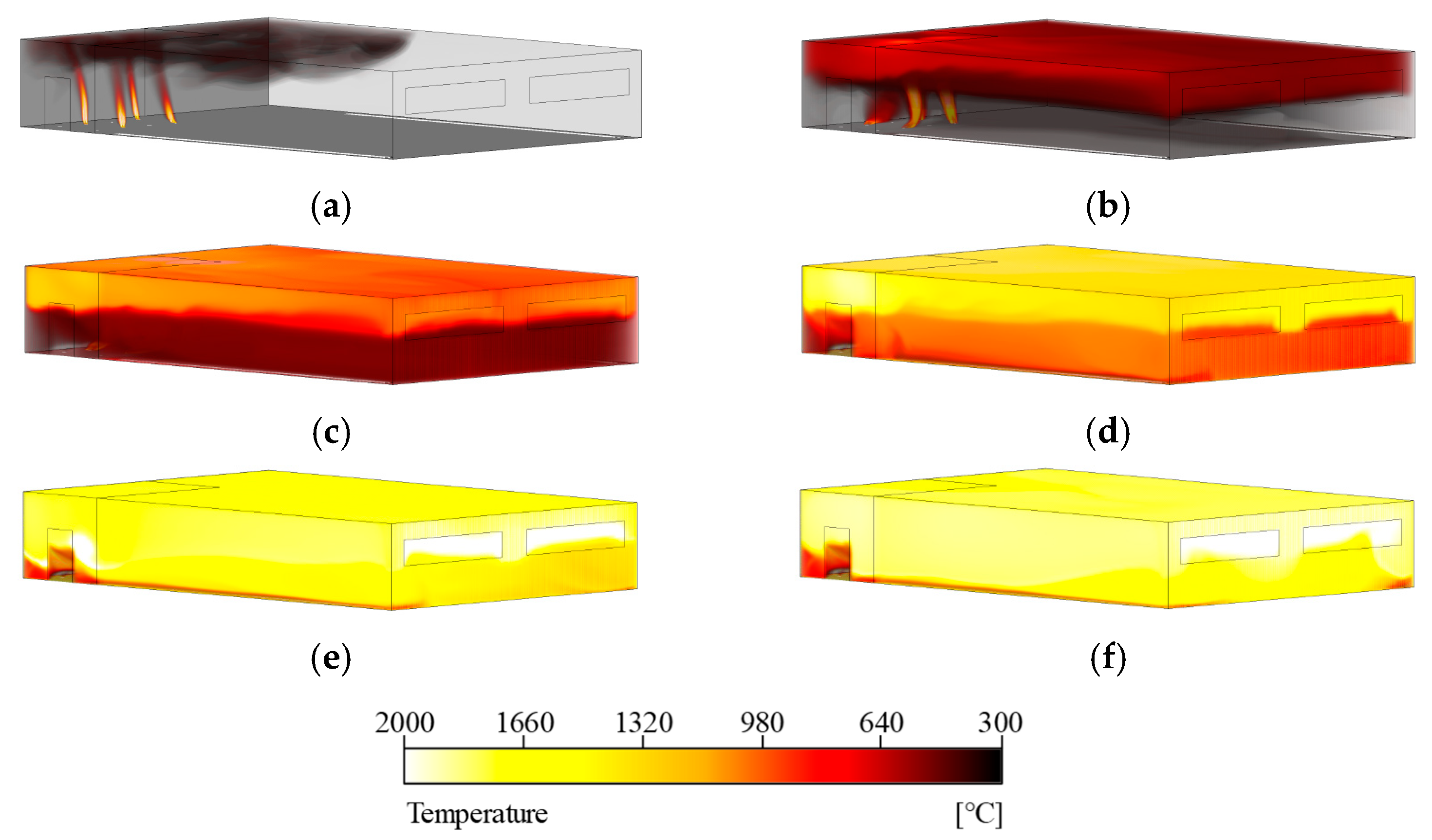
Figure 14 visualizes the three-dimensional temperature distribution within the compartment over time. From 70 s, approximately 10 s after the partition wall was removed, it was observed that hot gases generated by the fire rapidly spread throughout the compartment. Due to buoyancy effects caused by temperature differences, high-temperature regions initially developed near the ceiling and gradually descended as time progressed. A comparison of the temperature distributions at 600 s and 720 s showed similar thermal patterns, indicating that the compartment approached a quasi-steady state. 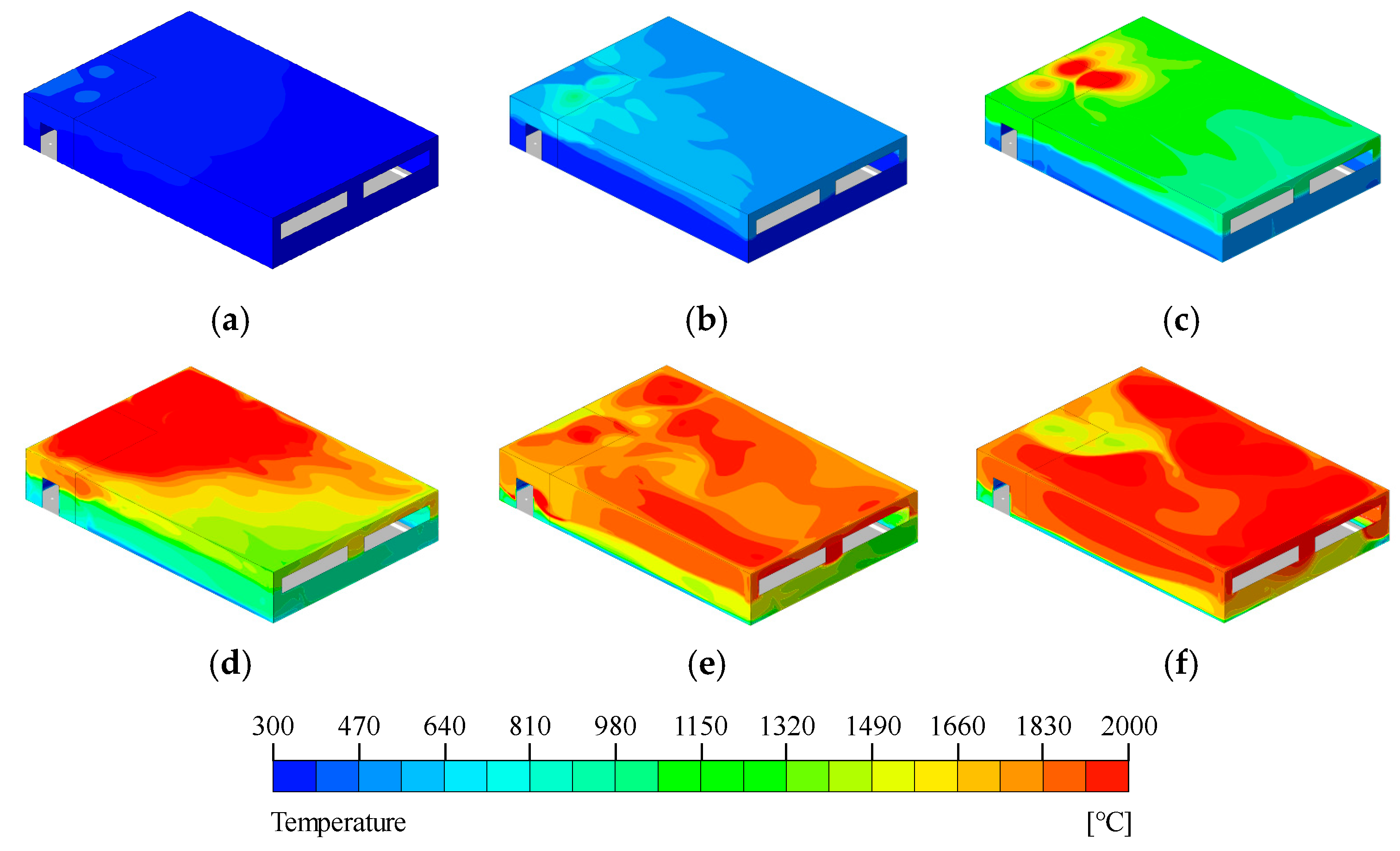In addition, as shown in Figure 15, the wall temperature increased beginning at the fire-exposed region directly impacted by the flames. After about 5 min of simulation, temperatures exceeding 2000 °C were observed on the upper wall surfaces. As the simulation continued, the influence of flame propagation caused a sustained increase in temperature across the entire wall surface. Subsequently, a numerical simulation was conducted by applying a User-Defined Function (UDF) to model pyrolysis phenomena and flame propagation within the compartment. The temporal variations in temperature at seven locations (T1–T7) are presented in Figure 16. The results showed that the temperature trends at each measurement point were similar depending on their height, and the overall compartment temperature continuously increased as the simulation progressed.

As shown in Figure 17, a localized high-temperature region formed around the ignition source during the first 30 s. Between 50 and 110 s, heat was observed to propagate along the ceiling. Once a critical temperature was reached, fuel was released from the wall surfaces, which promoted combustion and further elevated the temperature. The elevated temperature, in turn, induced additional fuel release through interaction with the walls. This chain reaction repeatedly resulted in relatively higher temperatures in corner regions where reactions were more intense. 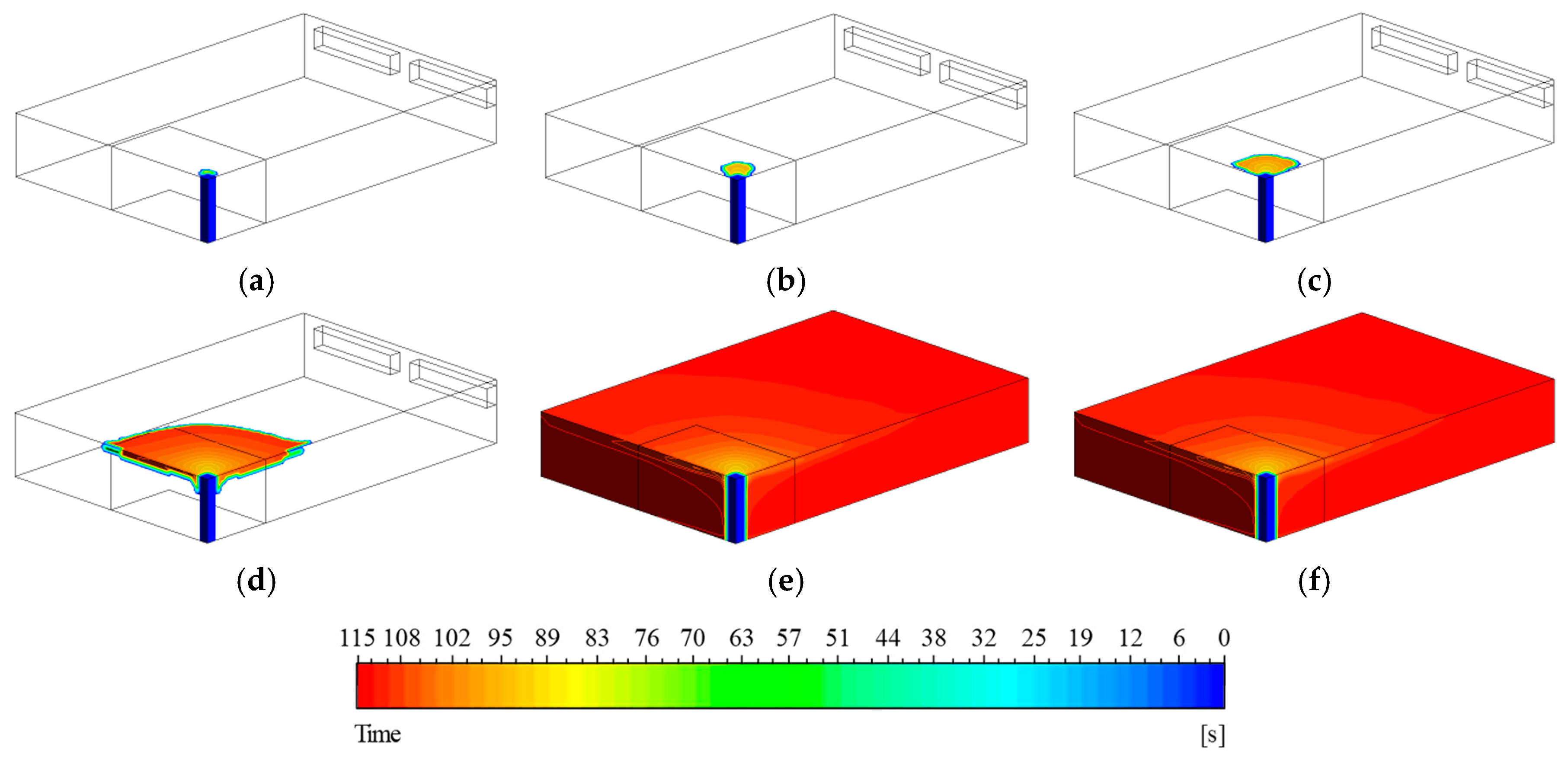The ignition timeline visualized in Figure 18 shows that after 100 s, flames rapidly spread across the ceiling, and by approximately 115 s, combustion occurred throughout the entire compartment. This phenomenon indicates a transition to a fully developed combustion state due to the rapid spread of pyrolysis and combustion reactions.

5. Conclusions

In this study, a pyrolysis model for combustible materials capable of analyzing ultra-fast fire behavior was developed and applied to investigate the characteristics of ultra-fast fires in industrial complex facilities. The main conclusions can be summarized as follows:

• To simulate the mass loss of matrix polymer specimens due to pyrolysis and combustion, the pyrolysis model was incorporated into the CFD analysis. This model predicts ignition and flame spread on solid surfaces and was implemented in ANSYS Fluent using User-Defined Functions (UDFs). As a result, the temporal mass variation in the specimen surface showed good agreement with experimental results, thereby validating the reliability of the model. Furthermore, this model was successfully applied to analyze the characteristics of ultra-fast fires in industrial complex facilities.
• In the analysis of Section 4.1.1 Simulations for Fire Growth Scenarios, a comparison was made between a constant HRR condition (1 MW) and a gradually increasing HRR condition (0 → 100 MW). Under the constant HRR condition, the internal HRR remained stable at approximately 1 MW, while the temperature continued to rise over time. In contrast, under the increasing HRR condition, the internal HRR stabilized at around 1 MW, but the external HRR continued to increase. This indicates that as the inflow rates of fuel and oxidizer increased, the dominant combustion reactions shifted from the internal to the external region. Consequently, the internal heat release reached a steady-state level, while additional combustion in the external region led to an overall increase in the total HRR.
• In the analysis of Section 4.1.2 Simulations of Flame Propagation in Full-Scale Enclosures, two conditions were considered. The first condition assumed that the HRR increased over time and that, one minute into the simulation, the partition wall was removed, allowing flames to spread throughout the entire domain. The second condition applied a User-Defined Function (UDF) to model fuel release from wall surfaces, where fuel was introduced into the compartment once a critical wall temperature was reached. The results showed that under the first condition, the temperature initially increased but dropped to lower positions once the partition was removed, before rising again as the HRR continued to grow. Similar temperature distributions were observed at the same vertical levels, attributed to buoyancy effects. Under the second condition, a high-temperature region initially formed near the ignition source, and as time progressed, flames rapidly propagated along the ceiling surface.

The pyrolysis model developed in this study enables the quantitative prediction and analysis of ultra-fast fire scenarios and is expected to serve as a useful tool for fire safety assessment and risk analysis in real industrial settings. In particular, the proposed model effectively reproduces high-temperature pyrolysis and rapid flame propagation characteristics, thereby providing practical contributions to fire simulations and the development of fire protection strategies for various industrial facilities in the future. Moreover, to enhance the applicability and accuracy of the model, further experimental and numerical validation that reflects diverse material properties and realistic fire environments will be required. Such efforts are anticipated to advance the model into a more reliable predictive framework.

References

- Fang, Y.; Qi, D.; Wu, L. Flame retardant cotton fabrics with ultra-fast and long-term fire early warning response. Int. J. Biol. Macromol. 2024, 271 Pt 1, 132673. [Google Scholar] [CrossRef] [PubMed]
- Saadet, A.; Ercument, A.; Kudret, A. Risk Assessment of Industrial Fires for Surrounding Vulnerable Facilities Using a Multi-Criteria Decision Support Approach and GIS. Fire 2021, 4, 53. [Google Scholar] [CrossRef]
- Yuri, M.; Fares, A.A.; Leonid, C.; Sergey, Z. Visualization of Hazardous Substance Emission Zones During a Fire at an Industrial Enterprise Using Cellular Automaton Method. Fire 2025, 8, 250. [Google Scholar] [CrossRef]
- Yuri, M.; Fares, A.A.; Olga, Z.; Sergey, Z. Simulation Modeling of the Process of Danger Zone Formation in Case of Fire at an Industrial Facility. Fire 2024, 7, 221. [Google Scholar] [CrossRef]
- BBC. Boss Arrested over Deadly Fire at S Korea Battery Plant. 2024. Available online: https://www.bbc.com/news/articles/c5y35nvvepwo (accessed on 25 August 2025).
- Maeil Business Newsletter. Fire at Auto Parts Factory. 2025. Available online: https://www.mk.co.kr/en/society/11319506 (accessed on 25 August 2025).
- Asia Business Daily. The Fire at Kumho Tire’s Gwangju Plant. 2025. Available online: https://cm.asiae.co.kr/en/article/2025060115464758710 (accessed on 25 August 2025).
- ISO 834; Fire Resistance Tests—Elements of Building Construction. International Standards Organization: Geneva, Switzerland, 1980.
- KS F 2257-1; Methods of Fire Resistance Test for Elements of Building Construction-General Requirements. Korea Standards & Certification: Seoul, Republic of Korea, 2019.
- Wang, Z.; Jia, F.; Galea, E.R.; Ewer, J. Computational fluid dynamics simulation of a post-crash aircraft fire test. J. Aircr. 2013, 50, 164–175. [Google Scholar] [CrossRef]
- Jiang, H.; Teng, J.; Wang, D.; Zhou, L.; Chen, Y. Numerical Investigation of the Wan’an Bridge Fire and the Protection Effect of Intumescent Flame-Retardant Coatings. Fire 2025, 8, 184. [Google Scholar] [CrossRef]
- Chen, X.; Wang, F. Performance-based engineering approach to accurately determine flame propagation characteristics over exterior video cladding wall. Fire Mater. 2021, 45, 690–696. [Google Scholar] [CrossRef]
- Snegirev, A.Y.; Kuznetsov, E.A.; Korobeinichev, O.P.; Shmakov, A.G.; Trubachev, S.A. Ignition and burning of the composite sample impacted by the Bunsen burner flame: A fully coupled simulation. Fire Saf. J. 2022, 127, 103507. [Google Scholar] [CrossRef]
- Ansys Fluent, Ansys Fluent Theory Guide; Ansys Inc.: Canonsburg, PA, USA, 2024; pp. 724–746. Available online: https://ansyshelp.ansys.com/public/account/secured?returnurl=/Views/Secured/corp/v242/en/flu_th/flu_th.html (accessed on 25 August 2025).
Figure 1.
Experimental setup: (a) Side view; (b) Top view.
Figure 2.
Correlation between CFD solver and pyrolysis model.
Figure 3.
Condition of analysis model: (a) Front view; (b) Side view.
Figure 4.
Section grids of analysis model: (a) Top view; (b) Side view.
Figure 5.
Transient variation in the sample mass [
13].
Figure 6.
Spatial distributions of conversion function : (a) t = 10 s; (b) t = 20 s; (c) t = 40 s; (d) t = 80 s.
Figure 7.
CFD Model geometry and dimensions conditions: (a) Side view; (b) Plan view; (c) Three-dimensional view.
Figure 8.
CFD Model geometry and dimensions conditions.
Figure 9.
Results of temperature and heat release rate (HRR).
Figure 10.
Temperature distribution of the simulation model: (a) Central cross-section of the simulation model, (b) Central cross-section of the fuel inlet.
Figure 11.
Results of temperature and heat release rate (HRR): (a) Temperature results by location, (b) Internal and external HRR results.
Figure 12.
Central cross-section temperature distribution of the simulation model: (a) analysis time 100 s, (b) analysis time 500 s.
Figure 13.
Results of temperature and heat release rate (HRR): (a) temperature results by location, (b) heat release rate (HRR).
Figure 14.
Internal temperature distribution of the simulation model: (a) t = 70 s, (b) t = 180 s, (c) t = 300 s, (d) t = 420 s, (e) t = 600 s, (f) t = 720 s.
Figure 15.
Temperature distribution on the walls of the simulation model: (a) t = 70 s, (b) t = 180 s, (c) t = 300 s, (d) t = 420 s, (e) t = 600 s, (f) t = 720 s.
Figure 16.
CFD Results of pyrolysis in the simulation model: (a) temperature and HRR results by location (T1~4), (b) external temperature of the fire compartment (T5~7).
Figure 17.
Temperature distribution on the wall of the simulation model: (a) t = 10 s, (b) t = 30 s, (c) t = 50 s, (d) t = 90 s, (e) t = 110 s, (f) t = 130 s.
Figure 18.
Distribution of ignition time on the wall surface: (a) t = 70 s, (b) t = 180 s, (c) t = 300 s, (d) t = 420 s, (e) t = 600 s, (f) t = 720 s.