The Role of Fuel Characteristics and Heat Release Formulations in Coupled Fire-Atmosphere Simulation

Abstract

In this study, we focus on the effects of fuel bed representation and fire heat and smoke distribution in a coupled fire-atmosphere simulation platform for two landscape-scale fires: the 2018 Camp Fire and the 2021 Caldor Fire. The fuel bed representation in the coupled fire-atmosphere simulation platform WRF-Fire currently includes only surface fuels. Thus, we enhance the model by adding canopy fuel characteristics and heat release, for which a method to calculate the heat generated from canopy fuel consumption is developed and implemented in WRF-Fire. Furthermore, the current WRF-Fire heat and smoke distribution in the atmosphere is replaced with a heat-conserving Truncated Gaussian (TG) function and its effects are evaluated. The simulated fire perimeters of case studies are validated against semi-continuous, high-resolution fire perimeters derived from NEXRAD radar observations. Furthermore, simulated plumes of the two fire cases are compared to NEXRAD radar reflectivity observations, followed by buoyancy analysis using simulated temperature and vertical velocity fields. The results show that while the improved fuel bed and the TG heat release scheme have small effects on the simulated fire perimeters of the wind-driven Camp Fire, they affect the propagation direction of the plume-driven Caldor Fire, leading to better-matching fire perimeters with the observations. However, the improved fuel bed representation, together with the TG heat smoke release scheme, leads to a more realistic plume structure in comparison to the observations in both fires. The buoyancy analysis also depicts more realistic fire-induced temperature anomalies and atmospheric circulation when the fuel bed is improved.

1. Introduction

Wildland fires can lead to substantial ecological, social, and economical losses [1] as well as health burdens due to smoke produced from biomass burning [2]. Affected by climate change and human activities, the frequency of wildfires has increased in recent years [3,4,5,6], leading to increased loss of life and property. Accurate wildfire simulations are an essential piece in predicting and managing these losses, benefiting both pre-fire risk mitigation and preparedness as well as active-fire emergency response management. However, accurate simulations require characterization and parametrization of the complex multi-physics nature of the fire combustion process including fire interactions with the atmosphere that can lead to localized fire-induced weather condition caused by fire generated heat [7]. To simulate fire–atmosphere interactions, coupled wildland fire-atmosphere simulation platforms have been developed, first of which was the work of Clark et al. [8], that showed empirical fire spread models coupled with atmospheric numerical models can reproduce the observed fire-weather characteristics.

Current coupled fire-atmosphere simulation platforms [9] are based on physics-based or semi-empirical approaches to model the combustion process for fire propagation simulation. While the physics-based models directly resolve fire combustion processes, and thus, represent the combustion process more realistically, they are hindered by high computational demand making their application limited to small-scale fires. In contrast, the coupled semi-empirical simulation platforms utilize semi-empirical fire spread models (e.g., Rothermel [10]) coupled with physics-based Numerical Weather Prediction (NWP) models. Therefore, their computational demand is lower than the physics-based simulation platforms, making them suitable for landscape-scale and operational fire simulations. One of these simulation platforms is the Weather Research and Forecasting-Fire (WRF-Fire) simulation platform [11,12] used in this study. In the WRF-Fire, the wind field is resolved by the WRF model and passed to the fire behavior model to compute the fire rate of spread (ROS) and the heat generated by combustion, which is then released into the WRF meteorological simulation to allow the fire to feed heat fluxes back into the atmosphere. The fire-generated heat is calculated based on the combusted mass of the simulation domain’s fuel bed, which currently consists of only surface fine fuels. Representing only the surface fuels in the simulation domain may lead to an inaccurate fire-weather simulation, as will be shown in our study. This is due to the fact that, in addition to surface fuels, canopy and course woody materials with significantly larger fuel loads than surface fuels (e.g., [13,14] for Sierra Nevada) and longer residence times (e.g., [15,16]) can burn during active fires. This can result in higher heat flux from the fire over a longer period of time, leading to more extreme atmosphere perturbations compared to surface fuels alone [17,18,19].

While various studies have been conducted to assess the performance of WRF-Fire in simulating landscape-scale fire behavior and its sensitivity to various modeling parameters and assumptions (e.g., [11,20,21,22,23,24,25,26,27]), no study exists that incorporates the parametrization of canopy and coarse woody materials in WRF-Fire to evaluate the relationship between fire energy and WRF-Fire simulated fire-weather. Kochanski et al. (2013) assessed the performance of WRF-SFIRE, which is a variation of WRF-Fire with the same fire behavior model, when simulating the FireFlux I prescribed burn [25]. The authors concluded that the ability of WRF-SFIRE to simulate the fire weather is reasonable. However, they increased the default fuel load value in WRF-SFIRE to almost three times to yield reasonable agreement between simulated and measured wind velocities and updraft. In another study by Mallia et al., a within-canopy wind profile model was implemented in WRF-SFIRE and its effects were examined in a simulation of the RxCadre prescribed burn [28]. While their results showed improved accuracy with the observations compared to the model without the canopy wind model, their study was limited to the within-canopy wind parametrization. Therefore, we highlight that no study exists that evaluates the sensitivity of the WRF-Fire simulated fire perimeter and smoke lofting height to fuel bed representation in a landscape-scale fire.

In light of this fire-atmosphere modeling gap, the objectives of this study are (1) to develop a new parametrization for crown fire heat release and a new scheme for fire generated heat and smoke distribution in the atmosphere for WRF-Fire, and (2) to investigate the sensitivity of fire perimeter, fire plume rise and transport, and fire-induced atmospheric circulation results of WRF-Fire to fuel bed representation in the simulation of two landscape-scale fires: a wind-driven fire (the 2018 Camp Fire) and a plume-driven fire (the 2021 Caldor Fire). The selection of a wind-driven and a plume-driven fire is influenced by the fact that the propagation of a wind-driven fire is mostly dictated by the ambient wind, whereas the propagation of a plume-driven fire is dictated by the fire plume. Hence, the latter is more sensitive to the fire heat fluxes than the former. Aside from the addition of new parametrizations in WRF-Fire, the outcomes of this study will lead to an improved understanding of fire feedbacks on the atmosphere, highlighting the challenges in coupled fire-atmosphere simulations, and guiding future directions in coupled fire-atmosphere simulation platform developments.

The structure of the paper is as follows. In Section 2, we start by introducing the study areas, WRF-Fire platform, and model setup. Next, the method developed for crown fire heat calculation, as well as the new heat and smoke distribution schemes are introduced. Section 2 is then concluded by our model setup for the Camp Fire and Caldor Fire. In Section 3, the simulated fire perimeters and plumes are compared with semi-continuous, high-resolution NEXRAD observations, and the simulated temperature and vertical velocity characteristics are compared with those observed during prescribed burns. Finally, we summarize results, discuss conclusions, and provide details of future directions in Section 4.

2. Methods

2.1. Study Area

2.1.1. Camp Fire as a Wind-Driven Fire

The Camp Fire started around 0620 PST on 8 November 2018 near the community of Pulga in Butte County, CA, USA, due to the failure of electrical transmission lines. With most of the damage occurring within the first day after ignition, it lasted for about 18 days, burning a total of 62,053 ha. The fire destroyed 18,804 structures and resulted in 85 civilian fatalities and several firefighter injuries. This fire was the most destructive and deadliest fire in California’s history and the costliest natural disaster worldwide in 2018 [29].

The Camp Fire area consists of Mediterranean California Mesic Mixed Conifer Forest vegetation cover based on LANDFIRE vegetation maps [30]. Therefore, the burned area is mainly composed of Ponderosa Pine (Pinus ponderosa), Jeffrey Pine (Pinus jeffreyi), Sugar Pine (Pinus lambertiana), Douglas Fir (Pseudotsuga menziesii), California White Fire (Abies lowiana), and incense cedar (Calocedrus decurrens). Furthermore, the Remote Automated Weather Stations (RAWS) observed wind speeds around 3 to 8 m s⁻¹ with gusts reaching 9 to 15 m s⁻¹ during the Camp Fire classifying this fire as a wind-driven fire [20].

In this study, the Camp Fire is simulated from 1300 to 2345 UTC, November 8, 2018. The simulation results are compared to semi-continuous, high-resolution fire boundaries and plumes identified from NEXRAD radar observations at 15 min intervals [31].

2.1.2. Caldor Fire as a Plume-Driven Fire

The Caldor Fire, which ignited near Omo Ranch in El Dorado County, CA, burned for 67 days. The fire burned 89,787 ha between August 14 and the end of October 2021 in the Northern Sierra Nevada and south of Lake Tahoe. The Caldor Fire destroyed ~1800 structures, and resulted in two non-fatal injuries [32]. It is the 15th largest and 16th most destructive wildfire in Californian history [33]. Detailed description of the events during the Caldor Fire can be found in [34].

Similar to the Camp Fire, the Caldor Fire area is mostly covered with Mediterranean California Mesic Mixed Conifer Forest based on LANDFIRE vegetation maps and a previous study [35]. However, compared to the Camp Fire, environmental winds were weaker during the period at which the Caldor Fire is simulated in this study. The Caldor Fire is simulated from 1545 to 2345 UTC 17 August 2021. During this period the RAWS in the area recorded wind speeds of approximately 0.5 to 2 m s⁻¹ with gusts reaching 3.5 to 6 m s⁻¹, resulting in a plume-driven fire in that period. Similar to the Camp Fire, the simulation results during this period are compared with NEXRAD-derived perimeters and plumes.

2.2. WRF-Fire and Model Setup

The Weather Research and Forecasting model (WRF) [35] is a widely used Computational Fluid Dynamics-based Numerical Weather Prediction model capable of multiscale atmospheric simulation bridging the mesoscale and microscale. In this study, we use the WRF-Fire model [11], which couples a fire behavior model to WRF, resulting in a fully coupled wildland fire-atmosphere simulation platform. WRF provides the fire behavior model with the atmospheric state, allowing it to calculate the fire rate of spread (ROS) based on the Rothermel ROS model [10], and thus propagate the fire on surface fuels using a level-set algorithm [36]. Once a model grid cell is ignited, its fuel mass loss is calculated at each time step, and the resulting sensible and latent heat fluxes are used to resolve the heat and moisture released from the fire into the atmosphere to simulate fire-generated weather. WRF-Fire can also simulate fire smoke emission, dispersion, and transport.

The model setup here for both the Camp and the Caldor Fires closely follows our previous studies [20,21,22,23], which is based on the Colorado Fire Prediction System (CO-FPS) model setup. In summary, the model utilizes two one-way nested atmospheric domains with a grid size of 1 km and 111 m in the outer and the inner domains, respectively, and 46 exponentially spaced vertical levels with the first level located ~7 m Above Ground Level (AGL). The fire behavior model grid size is set to be four times finer than the inner domain grid size (27.75 m) to better match the input fuel data obtained from LANDFIRE fuel maps, which has a resolution of 30 m. The surface fuel for the Camp and the Caldor Fire is assigned using Scott and Burgan 40 fuel categories [37] from LANDFIRE 2014 and 2021-capable fuel maps, respectively, which are the closes available fuel maps for each fire. To realistically represent the fuel moisture content (FMC), RAWS FMC measurements (retrieved from [38]) proximal to each fire is used. Thus, Jarbo Gap RAWS FMC records are used for the Camp Fire between 1300 and 2345 UTC, 8 November 2018, which is the simulation period of this fire. Similarly, Sugarloaf RAWS measurements between 1545 and 2345 UTC 17 August 2021 are used to determine the FMC for the Caldor Fire. Taking the mean of the measured FMC in the mentioned periods, the FMC is set to 4.7% and 5.92% for the Camp and Caldor Fires, respectively, and kept constant throughout the simulation. Compared to the default value of 8% FMC, these FMCs reflect notable fuel dryness conducive to rapid fire spread and high heat release. The timestep of the outer domain is 2 s for both cases while the inner domain timestep is 0.222 s for the Camp Fire and 0.111 s for the Caldor Fire to avoid numerical instabilities caused by large updrafts. The outer domain is parametrized with MYNN Level 2.5 [39] Planetary Boundary Layer (PBL) parametrization, and the inner domain is configured in Large Eddy Simulation (LES) mode with 3D 1.5-order Turbulent Kinetic Energy closure sub-grid scale mixing scheme [40]. The initial atmospheric and lateral boundary conditions are derived from ERA5 forcing data [41]. To represent the terrain, 30 arc second and 30 m resolution NASA SRTM topography maps are used for the outer and the inner domains, respectively. Further details on the model setup as well as WRF-Fire tutorials to generate inputs can be found in [20] and [42], respectively.

2.3. Fire Heat Representation in WRF-Fire

In WRF-Fire, the fire-atmosphere coupling (i.e., fire-generated weather) is simulated by the release of fire-generated sensible and latent heat fluxes to the WRF atmospheric model calculated using the following equations.

$$H_s=\frac{∆F}{∆t}\frac{1}{1+M_f}{w}_{l}h$$

(1)

$$H_l=\frac{∆F}{∆t}\frac{M_f+0.56}{1+M_f}{w}_{l}L$$

(2)

where $H_s$ (W m⁻²) and $H_l$ (W m⁻²) are sensible and latent heat fluxes, respectively, $∆F$ is the fraction of the fuel burned at the current timestep, $∆t$ (s) is the timestep size, $M_f$ is the fuel moisture content, $w_l$ (kg m⁻²) is the total fuel load including moisture, $h$ (J kg⁻¹) is the heat content of dry fuel, and $L$ (J kg⁻¹) is the specific heat of water condensation at 0 °C [12].

The flux divergences (i.e., the vertical gradient of heat fluxes) from the calculated sensible and latent heat fluxes from Equations (1) and (2) are inserted into the WRF atmospheric model as tendencies to the potential temperature and the water vapor prognostic equations, respectively. This scheme is currently used for surface fuels in WRF-Fire, and it will be also used for crown fire heat calculation and release in this study.

2.4. Canopy Heat Parametrization

As discussed in the Introduction, the fuel bed can be divided into (i) surface fine fuels, (ii) canopy fuels, and (iii) coarse down woody materials [43]. The current version of WRF-Fire considers only surface fine fuels for fire propagation and fire-induced atmospheric circulation simulation. While this may be suitable for fire propagation simulations, it may not be suitable for fire-induced atmospheric circulation simulation since canopy and coarse down woody materials can generate significant heat due to their significantly larger load and/or release heat over long periods because of their slower burning rate compared to surface fine fuels. To investigate this sensitivity and to represent the fuel bed more accurately in this study, the heat generated from the combustion of thermally thin canopy fuels is added to our simulations with several assumptions. The first assumption is that only thermally thin fuels of the canopy burn. This assumption is based on the rapid nature of this process, during which thermally thick canopy fuels, including 100 h and 1000 h fuels, may not receive a significant heat input to burn. This is in agreement with the definition of “crown fire” in the literature, which is also the basis of current crown fire propagation models (e.g., [44,45,46,47,48,49]). Therefore, the burning of thermally thin canopy fuels will be referred to as crown fire from this point forward. Nonetheless, the possibility of heat release due to the smoldering or glowing of thermally thick canopy fuels should be further investigated. The other assumption is that canopy preheating (i.e., time lag between canopy and surface fuel ignition) is not considered in this study due to a lack of proper data to correlate canopy preheating with surface fire heat fluxes. Following this, it is assumed that the surface fire can produce enough heat to ignite canopy fuel. Therefore, canopy fuel is ignited with the surface fuel. Additionally, the fire propagation (i.e., ROS) is calculated using surface fuels only by assuming that the surface fuels dominate the fire propagation due to their combustion characteristics. Future research is needed to further investigate these assumptions. It should also be noted that modeling heat release from coarse down woody materials is out of the scope of this study due to fundamental differences between these fuels and surface or canopy fine fuels such as smoldering burn over a long period.

Implementing crown fire in the WRF-Fire requires identifying canopy fuel characteristics, including canopy fuel load, mass loss rate, heat content, and FMC. Among the available data sources for canopy fuels (e.g., LANDFIRE and Forest Inventory Analysis), LANDFIRE canopy fuel maps are used to represent the canopy fuel load in this study. The LANDFIRE canopy fuel maps include canopy bulk density (CBD), canopy height (CH), and canopy base height (CBH). It should be noted that these data are not direct measurements. Instead, CBD is the output of a program known as “FuelCalc” [45], which calculates CBD using species-specific allometric relationships that relate CBD to crown characteristics such as diameter at breast height, canopy height and its ratio to live crown, canopy cover, and the number of trees per acre. Furthermore, CBH is the height at which CBD reaches 0.012 kg m⁻³, and CH is the output of a model that uses LANDSAT data and spatially explicit biophysical gradients [30]. Therefore, the canopy data likely includes modeling errors in addition to measurement uncertainties.

Using the LANDFIRE canopy parameters, the canopy fuel load (CFL) in kg m⁻² is calculated as follows.

$$CFL=CBD(CH-CBH)$$

(3)

It should be noted that the CFL calculated from Equation (3) only includes canopy fine fuel loads, which is the mass of foliage and half of the mass of twigs with diameters smaller than ~6 mm, based on the CBD definition. The calculated CFL together with the surface fine fuel load for the Camp Fire and Caldor Fire simulation domains are shown in Figure 1.

The heat from crown fire, as a result of burning CFL from Equation (3), is calculated using Equations (1) and (2), which require several more additional parameters. The dry canopy fuel heat content and FMC are assumed to be the same as surface fine fuels due to lack of observations. Therefore, the heat content is set to the heat content of dry fuel, which is equal to 17,433 kJ kg⁻¹. The calculation of thermally thin canopy fuel mass loss rate of the canopy is discussed in the following section.

2.5. Canopy Mass Loss Rate

Currently, WRF-Fire uses a simplified e-folding method derived from various experiments on woody pieces [15,50] to model rate of fuel consumption or mass loss rate. In this method, the mass loss rate is defined as an exponential function of time controlled by “fuel time”, which is the time required for the fuel to burn down to 36.89% of its original mass (see [12] for details). This mass loss rate scheme and the default fuel time values are used to burn the surface fine fuels in this study. For canopy fuels, however, this scheme is not valid due to the fundamental differences between canopy and surface fine fuels. For instance, surface fine fuels are compact and narrowly distributed in the vertical domain, whereas canopy fine fuels are diffuse and have a broader vertical distribution.

To address the canopy fuel consumption rate, we utilize the experiments conducted on Douglas Fir in [51] and Wildland Fire Dynamics Simulator (WFDS) [52] models of Ponderosa Pine from [53], which are two of the dominant species in the Camp Fire and the Caldor Fire domains as discussed in Section 2.1. The mass loss curve reported in the two previous studies are first shifted horizontally (i.e., along time axis) to omit the canopy heating and ignition periods for the experiments that have reported these periods since canopy preheating is not considered herein. Next, the Douglas Fir curves are shifted vertically (i.e., along the mass axis) with an initial tree mass that includes foliage mass and half of the twigs less than ~6 mm in diameter. The Ponderosa Pine curves are also shifted vertically to remove half of the mass of the twigs with diameters smaller than ~6 mm. This step is performed to make the curves compatible with the LANDFIRE CBD calculation scheme. All the curves are then normalized by the original mass of canopy fine fuels along the vertical axis to make the curves compatible with WRF-Fire fuel consumption calculations. Finally, the curves for both Ponderosa Pine and Douglas Fir experiments are used to fit an exponential curve for mass loss rate as follows.

$$F\left(t\right)=0.917e^{-0.07123t}+0.083$$

(4)

where $F\left(t\right)$ is the fraction of fuel remaining at time $t$, and $t$ is the time since grid ignition (s). The fitted curve achieves R² score of 92% and Root Mean Squared Error of 8%. Note that $F\left(0\right)=1$ initial condition. The fuel mass loss curves from the two previous studies, as well as the fitted exponential curves, are shown in Figure 2.

The fitted curve is implemented in WRF-Fire for this study to calculate the mass loss rate of the canopy fuel. It should be noted, however, that this mass loss rate calculation assumes that only Ponderosa Pine and Douglas Fir are present in the burn area. This assumption oversimplifies the burn characteristics of the canopy fuel by combining Ponderosa Pine and Douglas Fir burn characteristics and not considering other canopy characteristics such as canopy height. Further efforts are needed to address these shortcomings.

The heat generated from the crown fire together with the heat generated from the surface fine fuels are added to the atmospheric model as tendencies for fire-induced atmospheric circulation simulation. To avoid large vertical gradients in the heat flux and temperature that can result in numerical instability, the tendencies in WRF-Fire are distributed across vertical levels until a user-defined altitude (m AGL) known as the “heat extinction depth” (namelist option fire_ext_grnd) as will be discussed in the next section.

2.6. Heat Release Scheme in WRF-Fire

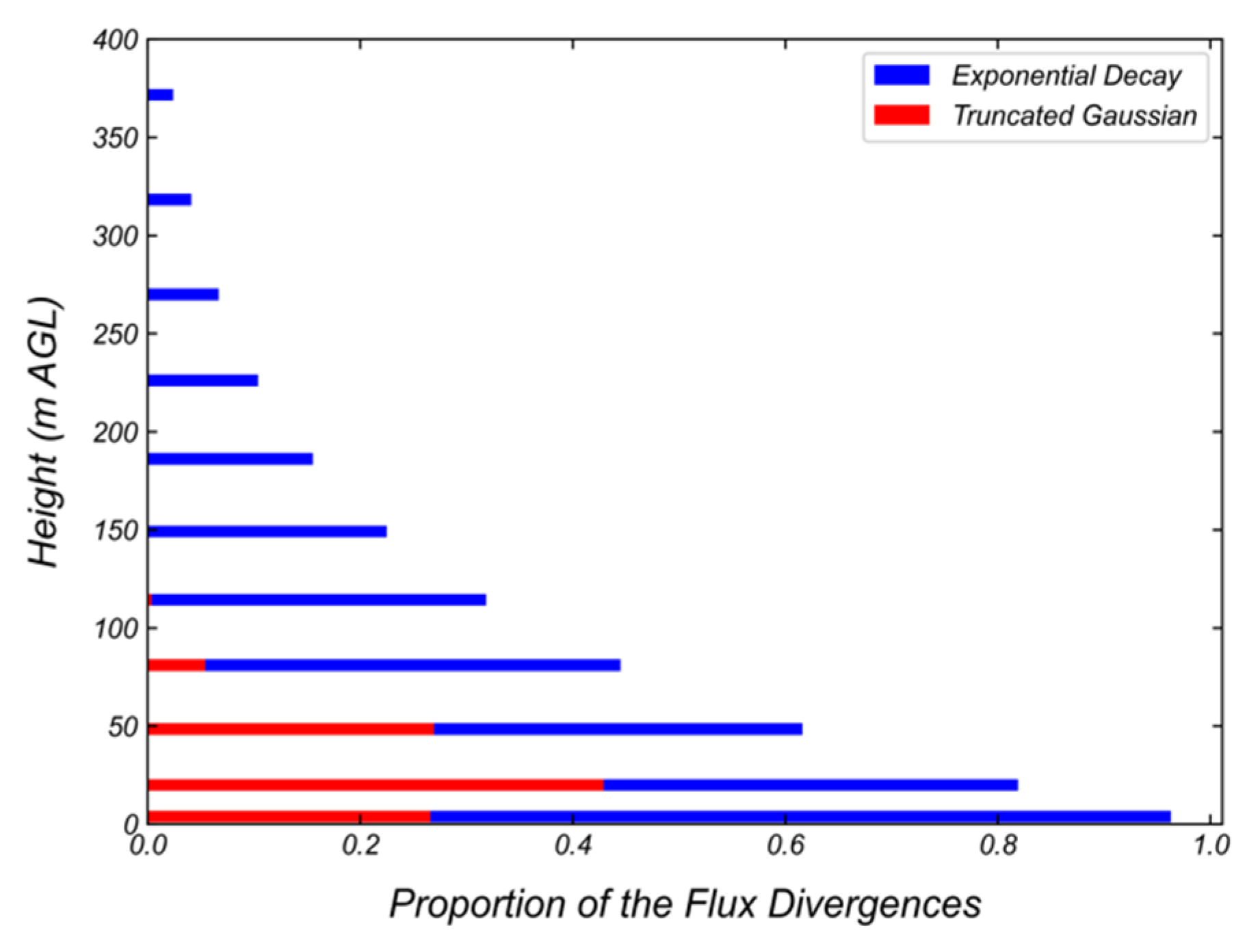
2.6.1. Original Heat Release Scheme

At present, in WRF-Fire, the heat fluxes from the modeled fire are distributed through the vertical levels using an exponential decay scheme by assuming that a simple radiation pretermination can be used to distribute the fire heat fluxes into the atmosphere [8,11] due to the lack of flux boundary conditions parametrization in WRF [12]. This exponential decay scheme is as follows.

$$P_i=e^{(-\frac{z_i}{z_{ext}})}$$

(5)

where $P_i$ is the proportion of the temperature and moisture flux divergences to be inserted at the ith vertical level located at $z_i$ AGL, and $z_{ext}$ is the heat extinction depth. The main issue with this formulation is that the total heat fluxes from the fire are not conserved, and they can be either magnified or reduced depending on the parameters of the scheme. For instance, Figure 3 shows the proportion of the flux divergences calculated using the exponential decay scheme with the heat extinction depth of 100 m for the model setup of this study. As can be seen, this scheme incorrectly magnifies the heat generated from the fire as the sum of the proportions of all vertical levels is equal to ~3.78.

2.6.2. Proposed Heat Release Scheme

To overcome the heat conservation issue of the current scheme, the following Truncated Gaussian (TG) scheme is proposed for the distribution of fire-generated sensible and latent heat in the atmospheric model. The choice of this functional form is influenced by the fact that Gaussian functions and their derivatives are smooth, and the function requires only two parameters, making it suitable to implement localized forcing or source (i.e., fire heat fluxes herein). Furthermore, the functional form integrates to one, allowing it to conserve the heat. The TG takes the following form.

$$p\left(\frac{z-\mu }{{0.5z}_{ext}}\right)=\left\{\begin{array}{c}\frac{2}{z_{ext}}\frac{\phi \left(\frac{z-\mu }{{0.5z}_{ext}}\right)}{\Phi \left(\frac{z_{max}-\mu }{{0.5z}_{ext}}\right)-\Phi \left(\frac{-\mu }{{0.5z}_{ext}}\right)} 0\le z\le z_{max}\\ 0 z>z_{max}\end{array}\right.$$

(6)

where $\mu$ (m AGL) is peak heat release elevation, z (m AGL) is elevation, $z_{max}$ (m AGL) is the upper bound of the function defined by the user and set to 1000 m in this study. Functions $\phi$ and $\Phi$ are calculated using:

$$\phi \left(x\right)=\frac{1}{2}(\alpha +3\beta x^2)(1-{tanh}^2(\alpha x+\beta x^3))$$

(7)

$$\Phi \left(x\right)=\frac{1}{2}(1+\mathit{tanh}(\alpha x+\beta x^3))$$

(8)

in which $\alpha$ and $\beta$ are constants set to 1.1284 and 0.1, respectively, so that the $\phi$ and $\Phi$ have similar characteristics as standard normal distribution and cumulative distribution functions, respectively, following [54].

The $p$ calculated from Equation (6) is a continuous TG Function. In order to apply the values of this distribution to discrete vertical levels of the WRF model, the continuous function is discretized using the following equation.

$$P_i=p(\frac{z_i-\mu }{{0.5z}_{ext}})∆z_i$$

(9)

in which, $∆z_i$ (m) is the ith vertical level spacing of the WRF model. This function assures the conservation of the fire heat fluxes when distributed through the vertical levels.

Furthermore, to allow for various forms of heat distribution schemes following the proposed TG function, the peak heat release elevation ($\mu )$ and extinction depth ($z_{ext})$ are set as user-defined parameters, and the effect of the peak heat release elevation is investigated in the case studies. A sample distribution using the proposed TG scheme for the model setup of this study is shown with red bars in Figure 3. In this figure, the peak heat release and extinction depth is set to 0 and 25 m, respectively. As can be seen, the TG scheme can preserve the heat released into the atmosphere unlike the exponential decay scheme. It should be noted that the shift in peak heat release location of this scheme in Figure 3 is due to the discretization of the continuous function in Equation (6) using Equation (9). The vertically stretching grid with refined vertical levels near the surface of this study model setup results in small $∆z_i$ near the surface compared to higher elevations.

2.7. Smoke Emission in WRF-Fire

In this study, WRF-Fire simulated smoke concentration is used to compare the atmospheric circulations with NEXRAD reflectivity data as a source of observation to study the effects of crown fire and the proposed TG scheme. In the current version of WRF-Fire, the fire smoke emission is simulated by releasing tracers at the first vertical level with values equal to 2% of the mass of the burned fuel at each timestep. This approach, however, poses two shortcomings. First, WRF-Fire currently does not simulate the concentration of different pollutants, such as Carbon Dioxide (CO₂), Particular Matter 2.5 (PM2.5), etc. It should be noted that WRF-SFIRE has this capability via coupling with WRF-Chem (e.g., [55,56]). Second, releasing the tracers at only the first vertical grid, which is usually less than 10 m AGL, is not realistic considering the heat release distribution and the height of burning canopy (if it exists). Addressing the first limitation is beyond the scope of this study. However, the second limitation is addressed by using the same TG distribution used for the heat release in the previous section. Therefore, the tracers are released across the height using the TG scheme discussed before. At each fire cell that is actively burning, 2% of the mass of the burned fuel at each timestep is distributed vertically until the extinction depth. This new TG smoke release scheme can possibly lead to more accurate simulation of the smoke emission (i.e., plume rise and transport) from fires, as will be shown later, which can be useful for mitigating wildfire impacts related to human health as well as decision support for fire suppression and management.

2.8. Sensitivity Studies

A series of case studies are conducted to investigate the effects of crown fire (i.e., improved representation of fuel bed) as well as the new TG heat release scheme, on fire propagation and fire-induced atmospheric circulation for the Camp Fire and the Caldor Fire.

Table 1. Summary of the case studies. LF and N/A in the table denote LANDFIRE and not applicable, respectively.

Fire	Case Name	Surface Fuel	Canopy Fuel	Heat Release Scheme	Extinction Depth (m)	Peak Heat Release (m)
Camp Fire	CampBase	LF 2014	N/A	Exponential Decay	100	N/A
	CampCan	LF 2014	LF 2014	Exponential Decay	100	N/A
	CampTGH1	LF 2014	LF 2014	Truncated Gaussian	100	0
	CampTGH2	LF 2014	LF 2014	Truncated Gaussian	100	25
Caldor Fire	CalBase	LF 2021 Capable	N/A	Exponential Decay	100	N/A
	CalCan	LF 2021 Capable	LF 2021 Capable	Exponential Decay	100	N/A
	CalTGH1	LF 2021 Capable	LF 2021 Capable	Truncated Gaussian	100	0
	CalTGH2	LF 2021 Capable	LF 2021 Capable	Truncated Gaussian	100	25

lists our experiments performed in this study and their assigned names and setups. We start with baseline cases: CampBase and CalBase for the Camp Fire and Caldor Fire, respectively. Baseline cases use only surface fine fuels based on LANDFIRE and the default heat and smoke release schemes. The heat extinction depth for the exponential decay scheme is set at 100 m for both cases. Our first set of sensitivity simulations, CampCan and CalCan, impose canopy fuel loads from the LANDFIRE 2014 and 2021-capable canopy datasets for the Camp and Caldor Fires simulations, respectively, to include crown fire heat in the simulations. In these cases, current WRF-Fire heat and smoke release formulation is used, which are exponential decay heat release and smoke tracers released at first vertical level. Next, we examine the effects of the proposed TG heat and smoke release scheme in Section 2.6.2. To this end, the heat extinction depth is set to 100 m to be the same as previous cases, and the sensitivity of the simulation results to the location of the peak heat release is investigated by assigning $\mu =0$ in CampTGH1 and CalTGH1 cases, and $\mu =25 \mathrm{m}$ in CampTGH2 and CalTGH2 cases.

3. Results

In this section the effects of the new parametrizations (i.e., crown fire heat and TG heat and smoke distribution) are investigated on the simulation results of Camp Fire and Caldor Fire. The simulated fire progression is investigated for the two fires followed by plume rise and transport analysis. Additionally, we provide buoyancy analysis for the Camp Fire to further investigate the plume rise and transport as well as the effects of the parametrization on the simulated temperature and vertical velocity. This analysis is not presented for the Caldor Fire due to the lack of measurements and similar patterns in the simulation results to the Camp Fire cases.

3.1. Camp Fire

3.1.1. Fire Progression

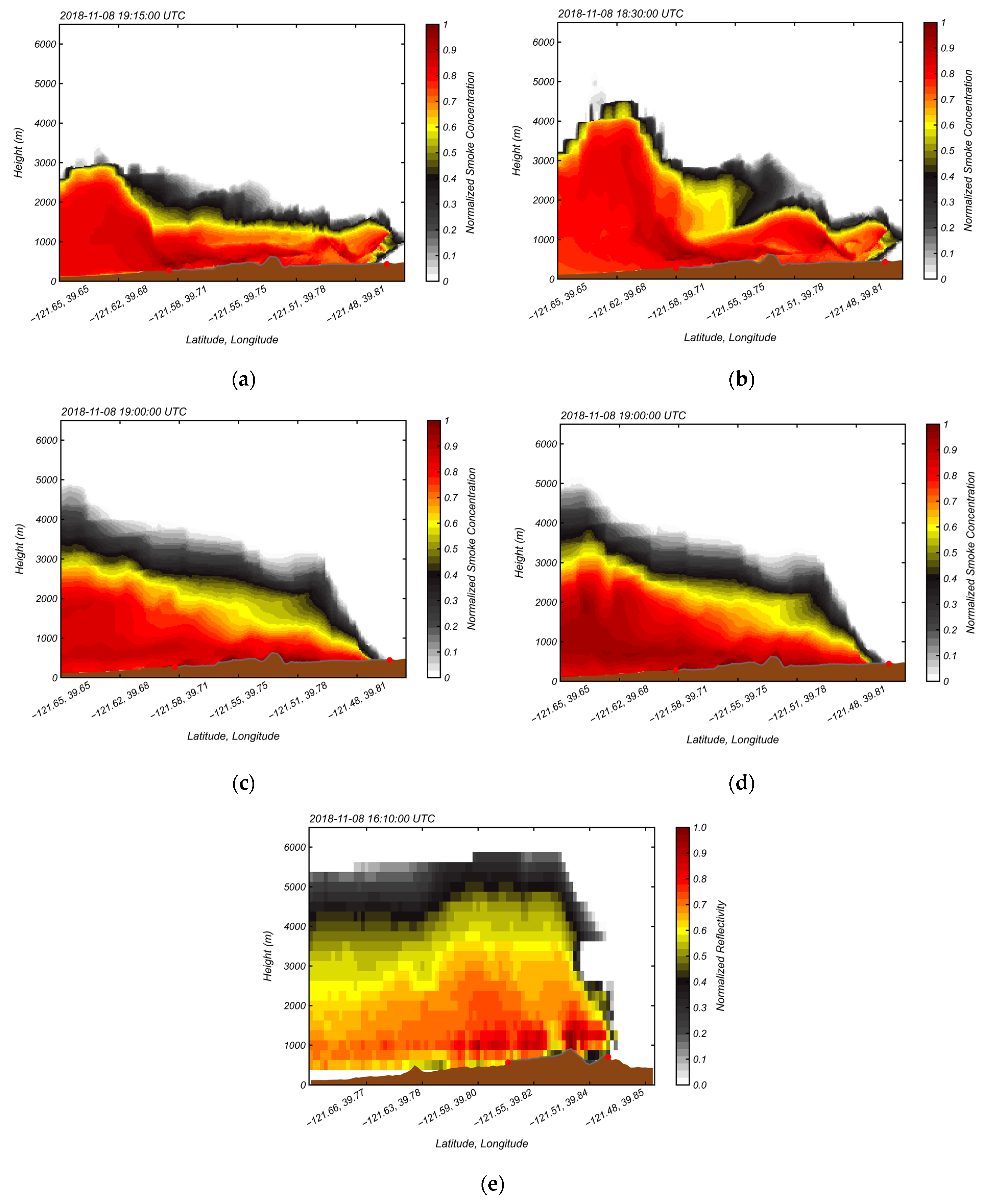
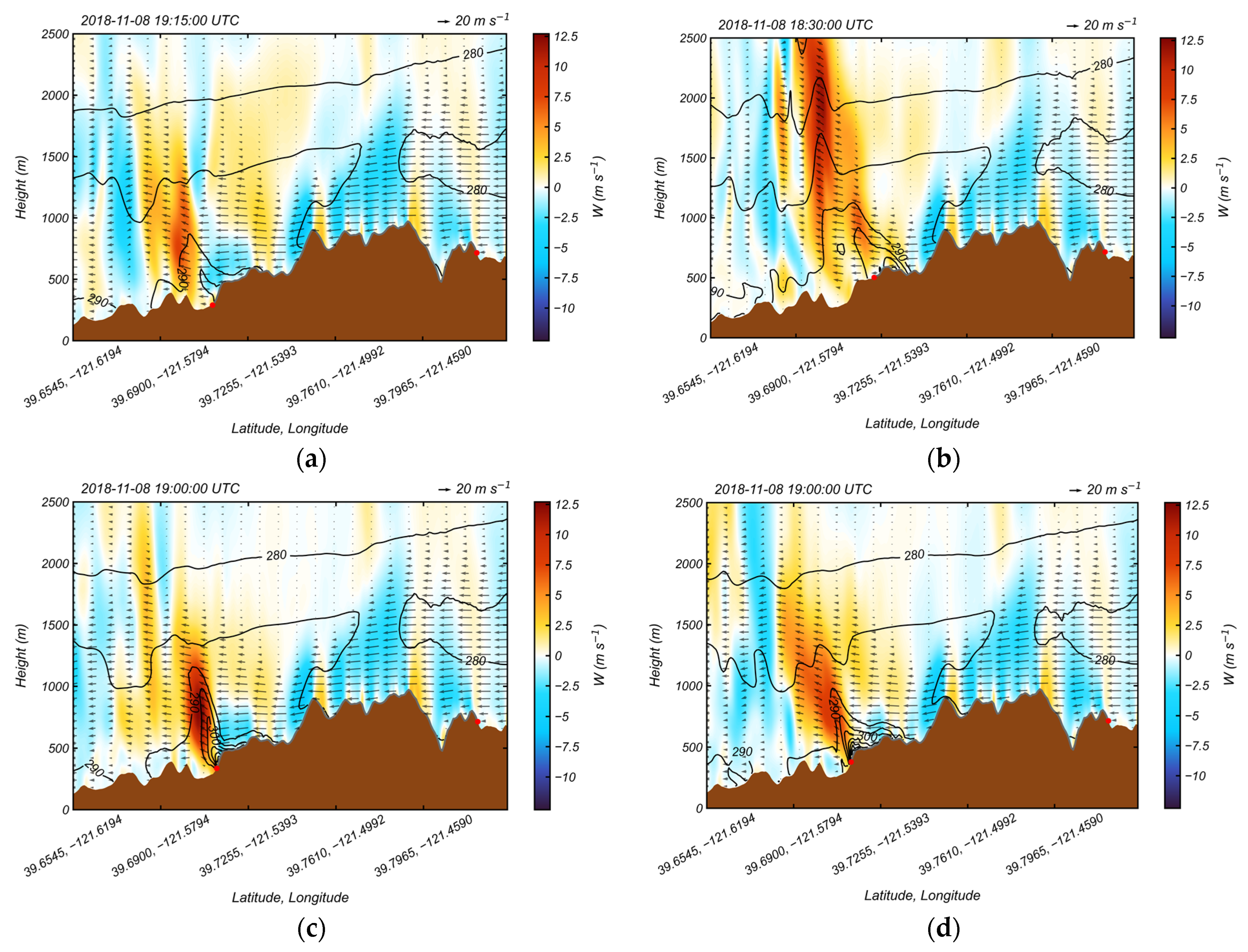
Camp Fire progression snapshots from the suite of simulations outlined in Table 1 are shown in Figure 4, and compared with estimated fire perimeters from NEXRAD observations [31]. Notably, while the simulated fire progression (colored lines) diverges from the radar-derived observations (gray shading), which will be called “the observations” from this point forward, the ROS between the cases varies, thus enabling a comparison amongst cases with different physics and fuel settings. The baseline case (CampBase, blue perimeter in Figure 4) propagates slower than the observations, especially during the first few hours of the simulation prior to 1900 UTC. Furthermore, the simulated fire erroneously slows down at the West Feather River Canyon near Paradise until 0015 UTC. In our previous study, we identified the possible source of this error to be an incorrectly simulated wind field at this canyon, which may be overcome by refining the atmospheric grid resolution to represent topography with finer details [20].

By modifying the fuel bed representation to include crown fire, the CampCan case (red perimeter in Figure 4) results in increased ROS compared to the CampBase case throughout the simulation. Compared to the observations, the fire, in this case, propagates with smaller ROS before 0015 UTC and with larger ROS after this time. Similar to the CampBase case, the fire, in this case, slows down at the valley, but it propagates uphill sooner at around 2215 UTC. Considering that only crown fire heat is added to this simulation compared to the CampBase case, the faster propagating fire, in this case, can be attributed to the effects of crown fire heat on the atmospheric circulation leading to strong fire-induced near-surface horizontal wind speed at the fire head directed toward propagation direction. This is evident in Figure S1, which shows the comparison of the simulated wind field of the CampBase and CampCan cases. Using the proposed TG heat release scheme, however, the simulated fire in the CampTGH1 (green perimeter in Figure 4) propagates at roughly the same ROS as the CampBase case, which is lower than the CampCan case, leading to the simulated fire head reaching the observed one around 1900 UTC. Furthermore, the CampTGH1 fire slows down at the canyon, similar to the CampBase and CampCan cases, and it propagates uphill roughly at the same time as the CampBase case at around 0015 UTC. The different fire propagation in this case compared to the CampCan case can be due to the conserved fire heat distributed in the atmosphere by the TG scheme, as the fuel bed is the same in both cases. In fact, Figure 3 shows that the exponential decay scheme magnifies the fire heat release by about ~237% of the fire-generated heat at <50 m AGL, which can lead to strong unrealistic fire-induced horizontal wind, and hence, larger ROS in the CampCan case. Moreover, this can also justify the approximately similar fire propagation between CampBase and CampTGH1 cases, as the fire in the CampTGH1 case has the added crown fire heat compared to the CampBase case. The CampTGH2 (magenta perimeter in Figure 4) case results in nearly identical fire propagation with the CampTGH1 case, which may show the insensitivity of the fire propagation to the mean value of TG scheme.

Overall, the fire propagation analysis for the Camp Fire suggests that the fire propagation is roughly insensitive to the added crown fire heat except for the CampCan case. In this case, however, the exponential decay heat release unrealistically magnified the heat generated from the fire when distributed in the atmosphere, which is physically inaccurate. The insensitivity of the fire propagation to the added crown fire can be due to the wind-driven nature of this fire as well as the effects of spotting as the fire propagation was mostly dictated by background wind and spotting during the Camp Fire.

Figure 4. Snapshots of fire progression of the Camp Fire case studies: (blue) CampBase, (red) CampCan, (green) CampTGH1, and (magenta) CampTGH2. Abbreviations are based on Table 1, and the black dashed line shows the location of the simulations vertical cross section of Section 3.1.2 and Section 3.1.3. The maroon dashed line indicates the cross-section location of NEXRAD reflectivity in Section 3.1.2. The radar-derived perimeters are shown with gray shading.

Figure 4. Snapshots of fire progression of the Camp Fire case studies: (blue) CampBase, (red) CampCan, (green) CampTGH1, and (magenta) CampTGH2. Abbreviations are based on Table 1, and the black dashed line shows the location of the simulations vertical cross section of Section 3.1.2 and Section 3.1.3. The maroon dashed line indicates the cross-section location of NEXRAD reflectivity in Section 3.1.2. The radar-derived perimeters are shown with gray shading.

3.1.2. Plume

NEXRAD radar reflectivity is sensitive to Pyrometeors [31,57], and thus can be used to validate simulated smoke plumes from the WRF-Fire. However, radar reflectivity is depicted in units of decibels relative to Z (dBZ), where Z is a quantity proportional to the size distribution and concentration of Pyrometeors [58], while WRF-Fire smoke concentration is depicted in units of smoke mass per unit mass of air. Due to the inherent differences in these two quantities, data pre-processing is performed to make them qualitatively comparable. First, a threshold of 10 dBZ is applied to the radar reflectivity to filter noise and non-smoke particles in the air. Similarly, the simulated smoke concentration is cut off at 1 ng to filter small smoke concentration values. Next, the simulated smoke concentration is converted into a logarithmic scale to have a comparable scale to the radar reflectivity dBZ unit. Lastly, both the radar reflectivity and simulated smoke concentration are normalized between zero and one using a min–max normalizer as follows.

$$X_{scaled}=\frac{X-X_{min}}{X_{max}-X_{min}}$$

(10)

where $X$ is either the radar reflectivity or smoke concentration. While a true quantitative comparison between the observed and simulated plumes is still not possible, the resulting data from the pre-processing steps can enable qualitative comparisons with the simulation results.

Figure 5a,d depict the vertical cross sections of the normalized smoke concentration of the Camp Fire simulations along the black dashed line in Figure 4, when the fire head is collocated in each case. The times when the fire head is collocated are identified by visual inspection of the 15 min interval vertical cross sections and plan view of the fire progression. These cross sections are the envelope of 61 cross sections 0.001 degrees apart with the black dashed line in Figure 4 being the middle one that captures the advancing fire head. This method is used to cover roughly the whole fire perimeter and to capture maximum plume concentration above the fire region. Using a similar approach for the observations, Figure 5e shows the vertical cross section of normalized NEXRAD reflectivity along the maroon dashed line in Figure 4 for the time when the fire head is located at the same longitude as the simulated cross sections determined by visual inspection of 5 and 15 min interval vertical cross sections of the observations and simulations, respectively. Nonetheless, it should be noted that this time is an approximation due to differences in fire propagation between the observed and simulated fire as well as the temporal resolution of the vertical cross sections.

As can be seen in Figure 5, the CampBase case (Figure 5a) has the shallowest plume among the cases, with a plume depth ~3 km above and downwind of the fire head and a ~1.8 to 2.5 km deep plume along the fire flanks. The inclusion of crown fire heat in the CampCan case (Figure 5b) yields a deeper plume, reaching ~4.5 km above and downwind of the head fire and 1.8 to 3 km along the flanks. This deeper plume stems from the added crown fire heat, which can cause increased buoyancy, especially above and downwind of the head fire leading to a larger plume rise (i.e., deeper plume). This will be further analyzed in the next section by analyzing the simulated temperature and vertical velocity. With the TG smoke distribution, the CampTGH1 and CampTGH2 cases (Figure 5c,d, respectively) achieve the deepest plumes among the cases with a ~3.4 km deep plume near the fire back, stretching to 5 km downwind of the fire head. Similar to the CampCan case, this deeper plume, compared to the CampBase case, can be due to the increased buoyancy caused by the added crown fire heat, as well as the TG smoke release scheme. However, compared to the CampCan case, the deeper plume can be largely attributed to the TG smoke distribution of these cases as the TG heat release reduces the amount of fire heat released in the atmosphere compared to the CampCan case as discussed in the previous section, which in turn can lead to decreased buoyancy and, hence, lower plume rise. The TG smoke distribution scheme in these cases, on the other hand, releases smoke tracers at vertical levels up to 100 m AGL compared to the CampCan case, in which the smoke tracers are released at ~7 m AGL (first vertical level). Therefore, a larger plume rise is expected in CampTGH1 and CampTGH2 cases as fire-induced updrafts should be weaker just above the surface than higher altitudes in these cases based on the expected fire plume dynamics described in [59]. This will be further analyzed in the next section by investigating fire-induced updraft.

Figure 5. Vertical cross sections of the normalized simulated smoke concentration for the Camp Fire (a) CampBase, (b) CampCan, (c) CampTGH1, and (d) CampTGH2 cases together with (e) normalized NEXRAD-observed reflectivity when the fire is located roughly at the same longitude. The brown shading shows the terrain. The gray line and the red circles show the burned area and the fire head, respectively. Abbreviations are based on Table 1.

Figure 5. Vertical cross sections of the normalized simulated smoke concentration for the Camp Fire (a) CampBase, (b) CampCan, (c) CampTGH1, and (d) CampTGH2 cases together with (e) normalized NEXRAD-observed reflectivity when the fire is located roughly at the same longitude. The brown shading shows the terrain. The gray line and the red circles show the burned area and the fire head, respectively. Abbreviations are based on Table 1.

Compared to the NEXRAD-observed reflectivity (Figure 5e), in which a 5 km deep plume is observed along the fire line and downwind the head fire, the CampTGH1 and CampTGH2 cases are in better agreement with the observed plume depth, whereas the CamBase case has the lowest agreement, and the CampCan case stands in between these cases. Nonetheless, all simulation cases underestimate the plume depth compared to the observations, which can be due to the lack of coarse down woody materials in the simulations. Further investigation of the simulated smoke concentration values reveals that, in all the cases, the highest smoke concentration occurs above and downwind of the fire head as well as in several scattered locations along the flanking fire line. This pattern is also evident in the observed reflectivity, with the difference that the observed reflectivity decreases as the distance from the fire head increases in the downwind direction. This can be partially due to the fall out of larger debris at this location, which is not captured by the simulations due to simplified smoke transport modeling in WRF-Fire that uses passive scalar tracers.

To expand our plume analysis beyond these snapshots, time-height plots of the maximum simulated smoke concentration and observed reflectivity are examined in Figure 6. These plots are prepared by taking the maximum value of the smoke concentration within 1.2 by 1.2 km squares around each pixel of the fire line at each vertical level and timestamp. Thus, these plots can enable validation of the simulation results for the simulation period rather than a single timestamp, as in Figure 5. After finding the maxima, the values are normalized using Equation (10). These data show the CampBase (Figure 6a) plume reaches ~3 and ~3.5 km prior to and after 1945 UTC, respectively. In the CampCan case (Figure 6b), while the plume stays below 3 km before 1800 UTC, similar to the CampBase case, the plume depth increases to an average of 5 km after this time with several spikes reaching ~7.5 km around 1930 UTC, when the fire is propagating with large ROS (see Figure 4). This is higher than the CampBase case, likely due to the buoyancy effects mentioned earlier for the snapshots. Unlike the other two cases, the CampTGH1 and CampTGH2 cases (Figure 6a,b) result in deeper plumes reaching >5 km between 1630 and 1815 UTC and average ~7 km with spikes reaching 8 and 8.6 km in the CampTGH1 and CampTGH2 cases, respectively, after 1815 UTC, likely due to the reasons mentioned earlier. Moreover, similar to the previous cases, these TG cases result in a shallow plume (<3 km) at the beginning of the simulation when the simulated fire is not well-established.

The time height plot of the maximum normalized radar reflectivity (Figure 6e) shows that the observed plume stays below 4 km before 1519 UTC followed by spikes to 7 km around 1545 UTC when the fire is well-established. Therefore, the shallow plume depth in the simulations when the fire is small agrees with the observed plume. However, only the CampCan, CampTGH1, and CampTGH2 cases can simulate the observed spike in the observed plume depth. Nevertheless, the occurrence time of the plume spike in these cases does not match the observation, which is due to the slower simulated fire spread compared to the observations during this period. In fact, investigation of Figure 4 shows that when the simulated fire starts to propagate with large ROS and the simulated burned area roughly matches the observed burned area, the spike in the plume depth occurs in the CampCan, CampTGH1, and CampTGH2 cases. This can be interpreted as a success for the cases with improved fuel beds. After this period, the observed plume depth decreases to around 4 km and remains roughly constant throughout the analyzed period. The plume depth at this period is overestimated by the CampCan, CampTGH1, and CampTGH2 cases, likely due to the coarse vertical resolution at high elevations (i.e., ~800 m between 7 and 8 km AGL).

Figure 6. Time height plots of the maximum normalized simulated smoke concentration over the simulation domain for the Camp Fire (a) CampBase, (b) CampCan, (c) CampTGH1, and (d) CampTGH2 cases together with the time height plot of (e) normalized NEXRAD-observed reflectivity. Abbreviations are based on Table 1.

Figure 6. Time height plots of the maximum normalized simulated smoke concentration over the simulation domain for the Camp Fire (a) CampBase, (b) CampCan, (c) CampTGH1, and (d) CampTGH2 cases together with the time height plot of (e) normalized NEXRAD-observed reflectivity. Abbreviations are based on Table 1.

3.1.3. Buoyancy Analysis

Accurate prediction of fire heat release and associated temperature increase, which results in enhanced buoyancy (i.e., vertical velocity), is essential for the accurate prediction of the plume rise as well as the atmospheric circulations at the head of the fire, potential wind convergence, and reverse flow that impact fire spread. Therefore, the simulated temperature and vertical velocity of the Camp Fire cases are investigated in this section. However, due to the lack of temperature and vertical velocity observations during the Camp Fire, the features of the simulated temperature and vertical velocity can be compared qualitatively with the features observed during prescribed burns experiments (e.g., [25,60,61,62,63,64,65,66]).

Figure 7 depicts the vertical cross sections of the simulated temperature and vertical velocity along black dashed line shown in Figure 4 for the Camp Fire cases for the same timestamp of plume cross sections in Figure 5. As can be seen in Figure 7, all cases show local temperature maxima at the proximal to the head fire wherein the temperature is decreasing with height above the surface. This temperature distribution is in agreement with the observation collected from FireFlux prescribed burn [65]. However, the magnitude and the structure of this peak temperature varies between the cases. While the CamBase case (Figure 7a) shows an increase in the temperature reaching ~300 K at the fire head, the increase is not significant compared to the ambient temperature (~290 K) unlike the pattern observed during the prescribed burns. In contrast, the CampCan, CampTGH1, and CampTGH2 cases (Figure 7b–d) exhibit a larger temperature increase to a maximum of ~305, ~315, and ~315 K, respectively, and they generate a wider area of temperature increase behind the fire head resulting in relatively better agreement with the prescribed burn observations.

In terms of the simulated vertical velocity, Figure 7 shows that all cases exhibit similar flow structures comprising increased horizontal wind preceding the head fire, weakly tilted updraft extending downwind of the head fire, and a downdraft region upstream of the head fire. This flow structure is consistent with those linked to prescribed fires [59], and an analysis of simulations without fire demonstrates they are fire-induced rather than terrain-induced features (Figure S2). The key difference in these simulations is the increased vertical velocity where the CampCan, CampTGH1, and CampTGH2 cases reach updrafts around 10, 12.5, and 7.5 m s⁻¹, respectively, as compared to ~7.5 m s⁻¹ in the CampBase case, which is likely due to the increased temperature perturbation from the fire caused by the addition of the crown fire heat. This analysis of the simulated temperature and vertical velocity shows enhanced buoyancy in the CampCan, CampTGH1, and CampTGH2 cases compared to the CampBase case, which can cause the plume to rise higher in these cases as shown earlier. Furthermore, it can be seen that the updraft magnitude around the head fire is weaker just above the surface compared to the higher altitudes in the cases, which is in agreement with the expected near-fire flow behavior described in [59]. This can also explain the deeper plume of the CampTGH1 and CampTGH2 cases compared to the CampBase and CampCan cases as the smoke tracers are distributed in the atmosphere, as mentioned earlier.

Further investigation of the simulated fire temperature and vertical velocity perturbations are accomplished using time-height plots of maximum temperature and maximum updrafts for the Camp Fire cases in Figure 8 and Figure 9. These plots are calculated by taking the maximum value of the temperature or updraft within 1.2 by 1.2 km squares around each pixel of the fire line at each vertical level, which is the same method used in the Plume section. As can be seen, the CampBase case (Figure 8a) achieves maximum temperatures of ~310 K at several time instances between 1845 UTC and 2045 UTC. In contrast, the CampCan, CampTGH1, and CampTGH2 cases (Figure 8b–d) achieve considerably higher maximum temperatures, reaching ~390, ~380, and ~380 K several times, which are likely more realistic compared to the CampBase case based on the pattern observed in the prescribed burns (e.g., [25,60,61,62,63,64,65,66]). The higher maximum temperatures of the CampCan case compared to CampTGH1 and CampTGH2 cases can be attributed to the unrealistically magnified fire heat fluxes by the exponential decay scheme.

Examining the time-height plots of the maximum updrafts of the Camp Fire cases depicts a pattern consistent with the temperature and plume analyses. The CampBase case (Figure 9a) achieves lower maximum updraft values than the cases with added crown fire (Figure 9b–d), with the CampCan case achieving the highest updraft values throughout the simulation. The maximum updrafts in the CampBase case are capped at ~12 m s⁻¹, while the maximum updrafts in the CampCan, CampTGH1, and CampTGH2 cases reach values above 30, 25, and 25 m s⁻¹, respectively. The maximum updrafts values obtained in these cases are more comparable to the FROSTFIRE crown fire experimental burn in [66] in contrast to the CampBase case. Similar to the cross-section snapshots, these simulated maximum temperatures and updrafts depict a greater buoyancy in the cases with added crown fire (CampCan, CampTGH1, and CampTGH2 cases) compared to the CampBase case, which can explain the deeper plumes achieved in the crown fire cases. Additionally, the higher maximum updrafts in the CampCan case compared to the CampTGH1 and CampTGH2 can show the effects of the unrealistically magnified fire heat fluxes by the exponential decay, similar to the pattern observed in the temperature analysis. Furthermore, closely following the cross-section snapshots, the maximum updrafts are weaker just above the surface than the higher elevations in all cases, likely leading to the deeper plume observed in the cases with TG smoke distribution compared to the other cases.

Figure 8. Time height plots of the maximum simulated temperature (T) over the simulation domain for the Camp Fire (a) CampBase, (b) CampCan, (c) CampTGH1, and (d) CampTGH2 cases. Abbreviations are based on Table 1.

Figure 8. Time height plots of the maximum simulated temperature (T) over the simulation domain for the Camp Fire (a) CampBase, (b) CampCan, (c) CampTGH1, and (d) CampTGH2 cases. Abbreviations are based on Table 1.

In summary, the plume and buoyancy analysis show that the inclusion of crown fire heat in the Camp Fire simulations results in improved prediction of plume depth compared to the radar observations, due to increased buoyancy by fire heat fluxes. That is, the addition of crown fire heat in simulations lead to stronger fire-induced updraft which is associated with larger temperature anomalies in the atmosphere by the fire. Furthermore, the addition of the TG heat and smoke distribution schemes results in further improvements in the prediction of fire plume and fire-induced buoyancy, respectively.

Figure 9. Time height plots of the maximum simulated updraft (W) over the simulation domain for the Camp Fire (a) CampBase, (b) CampCan, (c) CampTGH1, and (d) CampTGH2 cases. Abbreviations are based on Table 1.

Figure 9. Time height plots of the maximum simulated updraft (W) over the simulation domain for the Camp Fire (a) CampBase, (b) CampCan, (c) CampTGH1, and (d) CampTGH2 cases. Abbreviations are based on Table 1.

3.2. Caldor Fire

3.2.1. Fire Progression

Figure 10 depicts snapshots of fire progression of the Caldor Fire case studies outlined in Table 1. Unlike the Camp Fire cases, the baseline case, CalBase (blue perimeter in Figure 10) exhibits similar ROS and spread direction compared to the observations (gray shading) until 1800 UTC. Despite the overall agreement, the simulated fire head falls behind the observations after 2000 UTC, when the fire accelerates, and it propagates northeasterly rather than easterly in the observations leading to roughly 30 degrees propagation direction difference. Similar to the Camp Fire simulations, inclusion of crown fire heat (CalCan, red perimeter in Figure 10) yields to a faster propagating fire that almost matches the observed ROS in all directions throughout the simulations. This can be due to higher fire heat in this case compared to the CalBase case due to added crown fire heat, leading to stronger winds at fire head and localized fire-induced circulation. In terms of spread direction, however, the CalCan case propagates similar to the CalBase with a correct direction before 2000 UTC and somewhat errant (e.g., more northeasterly rather than easterly) direction after this time as compared with observations.

Adding the TG heat release (0 m and 25 m mean) in the CalTGH1 and CalTGH2 cases (green and magenta perimeters in Figure 10), respectively, results in almost identical simulated fire perimeters with CalCan case prior to 2100 UTC. After this time, these cases have a more easterly propagation compared to the northeasterly propagation in the CalCan case, which is in somewhat better agreement with the observations. This likely indicates the importance of local fire-induced atmospheric circulation in the simulation platform. In fact, taking into account that the distributed fire heat fluxes in the atmosphere are lower in the CalTGH1 and CalTGH2 cases than the CalCan case and that this fire is plume-driven, the propagation direction difference of these cases can be attributed to the lower heat fluxes leading to weaker fire plumes (i.e., less buoyant plumes) especially at the northeast head fire, where the plume is stronger than fire flanks (i.e., east side of the perimeter). This weaker plume can have a lower influence on the wind field compared to the CalCan case, which in turn can allow possibly weaker fire plumes on the east side of the fire perimeter to have stronger influence on their surrounding wind field changing the wind direction towards the east (i.e., toward the fire plume); hence, leading to the more easterly propagation in this case. This phenomenon was not observed in the Camp Fire simulations, which can be due to the wind-driven nature of fire causing the wind to dictate the propagation direction rather than the fire plume. Moreover, the CalTGH1 and CalTGH2 cases achieve roughly the same ROS as the CalCan case in all direction, which are in better agreement with the observations than the CalBase case.

Overall, the fire progression of the Caldor cases suggests that improving the fuel bed representation results in slightly better agreement with the observations, and adding the proposed TG heat release slightly improves the propagation direction. Following the analysis approach for the Camp Fire, the simulated plume, temperature, and vertical velocity are investigated in the following sub-sections.

Figure 10. Snapshots of fire progression of the Caldor Fire case studies. Abbreviations in the legend are based on Table 1, and the black dashed line shows the location of the vertical cross section of Section 3.2.2. The radar-driven perimeters are shown with gray shading.

Figure 10. Snapshots of fire progression of the Caldor Fire case studies. Abbreviations in the legend are based on Table 1, and the black dashed line shows the location of the vertical cross section of Section 3.2.2. The radar-driven perimeters are shown with gray shading.

3.2.2. Plume

Similar to the Camp Fire analysis, the simulated smoke plumes are compared with NEXRAD observations of the Caldor Fire. We begin by examining cross sections of the simulated normalized smoke concentration of the Caldor Fire cases depicted in Figure 11a to 11d for an envelope of 0.001 degree apart cross sections surrounding the transect shown by a dashed line in Figure 10 to roughly capture the whole fire perimeter including the head fire. This is the same approach utilized for the Camp Fire analysis. These data show a large disparity between the maximum plume depth in CalBase case (~4.7 km, Figure 11a) and the CalCan, CalTGH1, and CalTGH2 cases, which yield 6–7 km deep plumes (Figure 11b–d) likely stemming from the increased buoyancy by the added crown fire heat (see Figure S3). Additionally, all the simulation cases show a plume that rises vertically at the fire head until the plume top reaches a certain elevation, at which it is not buoyant anymore due to thermal stability, before sinking downwind. This behavior is encouraging, as it agrees with the expected plume structure of plume-driven fires. It is worth mentioning that this is different than the plume rises and transport in the Camp Fire simulations, as the primary driver of the plume transport was the strong ambient wind leading to lower vertical rise before being advected downwind.

Compared to the NEXRAD observations, the CalCan, CalTGH1, and CalTGH2 cases all compare favorably with the NEXRAD observations (Figure 11e) in terms of plume height and qualitative plume structure, although the observed plume is deeper than in all of the simulations (i.e., average 7.5 km deep observed plume), which can be due to the lack of coarse down woody materials in the simulation. The deeper plume of these cases can be attributed to more buoyant plume in these cases compared to the CalBase due to the added canopy heat flux closely following the pattern observed in the Camp Fire simulations. However, unlike the Camp Fire where the addition of TG smoke release led to a deeper plume, the addition of TG smoke release in CalTGH1 and CalTGH2 cases results in roughly the same plume depth as in the CalCan case. A possible reason for this is the vertical rise before horizontal advection of the plume in this fire as discussed earlier. Unlike the CalCan case, however, the CalTGH1 and CalTGH2 cases present higher smoke concentration roughly below 4 km, which is in better agreement with the observations than the CalCan case. This can stem from the TG smoke distribution which, as discussed in the Camp Fire simulation, releases the smoke tracers at higher elevations where strong fire-induced circulation leads to large updrafts aiding the plume rise.

To expand the plume analysis, time-height plots of the maximum simulated normalized smoke concentration for the Caldor Fire cases are shown in Figure 12a–d. The maximum plume depth of the CalBase case (Figure 12a) is 3 km AGL until 1845 UTC and ~4.7 km AGL from this time until the end of the simulation. In contrast, the maximum plume depth in the CalCan case (Figure 12b) reaches around 9 km AGL at several time stamps and averages at 6.4 km AGL throughout the simulation, which is likely due to the added crown fire heat leading to increased buoyancy (see Figures S4 and S5) similar to the Camp Fire simulations. Closely following this case, the plumes in CalTGH1 and CalTGH2 cases (Figure 12c,d) reach ~8 km AGL and ~9 km AGL, respectively, at several time stamps and average at ~6 km AGL in both cases. This pattern is contrary to the Camp Fire cases, where the CampTGH1 and CampTGH2 cases resulted in deeper plumes compared to the CampCan case. However, unlike the Camp Fire simulations, the Caldor Fire is a plume-driven fire, in which, as mentioned earlier, the plume first rises vertically until it is no longer buoyant. This can explain the similar maximum plume depths in the cases with added crown fire heat as the atmospheric potential temperature profile is likely affected less by the fire at 7–8 km AGL compared to the lower elevations.

Comparison of the simulated results with the time height plot of the maximum radar reflectivity (Figure 12e) supports our inferences from the snapshot cross-sections. Namely, there is much better agreement between observations and the mean and maximum plume depths in the CalCan, CalTGH1, and CalTGH2 cases as compared with the baseline case. Nevertheless, the underestimation of the plume depth observed in the snapshots is also evident in the time-height plots. Further investigation of the results shows that the simulated maximum normalized smoke concentration values in the CalTGH1 and CalTGH2 cases below 2 km AGL match the observations better compared to the CalCan case. This can be attributed to the TG smoke scheme of these cases releasing smoke tracers at higher elevations, where fire-induced updrafts are stronger, compared to the original scheme in WRF-Fire, which releases the tracers at the first level (~7 m AGL).

Figure 11. Vertical cross sections of the normalized simulated smoke concentration for the Caldor Fire (a) CalBase, (b) CalCan, (c) CalTGH1, and (d) CalTGH2 cases together with (e) normalized NEXRAD-observed reflectivity when the fire is located roughly at the same location. The brown shading shows the terrain. The gray line and the red circles show the burned area and the fire head, respectively. Abbreviations are based on Table 1.

Figure 11. Vertical cross sections of the normalized simulated smoke concentration for the Caldor Fire (a) CalBase, (b) CalCan, (c) CalTGH1, and (d) CalTGH2 cases together with (e) normalized NEXRAD-observed reflectivity when the fire is located roughly at the same location. The brown shading shows the terrain. The gray line and the red circles show the burned area and the fire head, respectively. Abbreviations are based on Table 1.

Figure 12. Time height plots of the maximum normalized simulated smoke concentration over the simulation domain for the Caldor Fire (a) CalBase, (b) CalCan, (c) CalTGH1, and (d) CalTGH2 cases together with (e) time height plot of normalized NEXRAD-observed reflectivity. Abbreviations are based on Table 1.

Figure 12. Time height plots of the maximum normalized simulated smoke concentration over the simulation domain for the Caldor Fire (a) CalBase, (b) CalCan, (c) CalTGH1, and (d) CalTGH2 cases together with (e) time height plot of normalized NEXRAD-observed reflectivity. Abbreviations are based on Table 1.

In summary, the plume analysis indicates that the improved fuel bed leads to closer-to-reality plume depth and that using the TG scheme for the smoke release can lead to further yet slight improvements in the simulated plume compared to the observations. Indeed, our analyses of the temperature and vertical velocity structure of the Caldor plume (available in Figures S4 and S5) support these inferences and point to a similar conclusion as in the Camp Fire cases. That is, the improved fuel bed representation produces larger temperature anomalies and correspondingly larger vertical velocities resulting in increased buoyancy and, in turn, more realistic plume depth in comparison to the cases with only surface fuels.

4. Conclusions

This study used NEXRAD observations and a coupled fire-atmosphere model, WRF-Fire, to examine the sensitivity of fire progression, as well as smoke plume rise and depth resulting from fire-generated heat to fuel bed representation and fire heat release formulation. To this end:

• A new parametrization to calculate the heat from the combustion of thermally thin canopy fuels was developed for the WRF-Fire using canopy burn experiments and physics-based simulations in the literature;
• An improved formulation to distribute fire-generated heat fluxes into the atmosphere was developed using a Truncated Gaussian (TG) functional form to overcome the heat conservation issue of the original heat distribution scheme of WRF-Fire;
• The proposed TG heat distribution scheme was also used to release fire smoke tracers in the atmosphere to account for the effects of fuel height, which can vary significantly depending on the fuel structure (i.e., various combinations of surface and canopy fuels).

The effects of the aforementioned new parametrizations were investigated in WRF-Fire simulations of a wind-driven fire, the 2018 Camp Fire, and a plume-driven fire, the 2021 Caldor Fire, using a series of sensitivity cases and baseline cases. For the baseline cases, we used default WRF-Fire options; that is, a fuel bed that includes only surface fine fuels, an exponential decay heat release scheme, and smoke tracers released at the first vertical level. The simulated fire progression of the cases was then compared to semi-continuous, high-resolution fire perimeters estimated from NEXRAD observations, and the simulated plume rise and transport of the cases were analyzed using NEXRAD reflectivity observations. The analysis was further accompanied by buoyancy analysis using the simulated temperature and vertical velocity.

Figure 13 depicts the simulated and observed burned area for both the Camp Fire and Caldor Fire. This figure and the fire progression analysis suggested that the simulated fire progression results of wind-driven fires are likely insensitive to the crown fire heat as these fires are mostly governed by the background and fire spotting. However, in the case of plume-driven fires, the inclusion of the combustion heat of other fuel types (e.g., canopy fuel) can have large effects on the propagation results as these fires are governed by the fire plume. Specifically, the simulated fire perimeters and burned area of the CampBase, CampTGH1, and CampTGH2 cases were roughly the same, although the CampTGH1 and CampTGH2 cases included canopy fuels in addition to surface fine fuels; hence, larger fire-generated heat fluxes due to added crown fire heat. It should be noted that while the CampCan case resulted in a faster propagating fire and higher burned area than the other cases, the exponential decay heat release scheme of this case was unrealistically magnifying the fire heat fluxes leading to unrealistic fire propagation results. Unlike the Camp Fire cases, the Caldor Fire case’s fire perimeters and burned area depicted a larger sensitivity to the fire heat fluxes, where the cases with added crown fire heat and TG heat release scheme propagated with different directions and larger burned area compared to the baseline case (CalBase) in better agreement with the NEXRAD-derived fire perimeters. This is expected, as the primary driver of the plume-driven fires is the fire-induced atmospheric circulations by their plume, whereas in wind-driven fires, the primary driver of the fire is the ambient wind.

Unlike the fire progression analysis, the fire plume analysis in both fires favored the cases with added crown fire heat as well as TG smoke heat and smoke release scheme.

Table 2. Summary of the simulated and observed plume depth as well as fire-induced temperature and updraft maxima for the Camp Fire and Caldor Fire. N/A denotes not applicable.

Fire	Case	Maximum Plume Depth (km)	Average Plume Depth (km)	Maximum Temperature (K)	Maximum Updraft (m s−1)
Camp Fire	NEXRAD	6.57	4.08	N/A	N/A
	CampBase	4.61	3.45	310	12
	CampCan	7.61	4.55	395	32.8
	CampTGH1	8	6.53	380	25.8
	CampTGH2	8.59	6.61	383	27
Caldor Fire	NEXRAD	12.34	6.66	N/A	N/A
	CalBase	4.79	3.52	310	17.1
	CalCan	8.89	6.4	368	35.3
	CalTGH1	8	5.98	357	33.5
	CalTGH2	9.17	6.18	361	34.1

summarizes the simulated and observed plume depth together with the fire-induced temperature and updraft maxima for both Camp Fire and Caldor Fire. Based on this table and the results discussed in Section 3, the cases with added crown fire heat using the original WRF-Fire heat and smoke distribution (i.e., the CampCan and CalCan for the Camp Fire and Caldor Fire, respectively) yielded higher plume depth compared to their respective baseline cases (i.e., the CampBase and CalBase) in better agreement with the NEXRAD-observed reflectivity. This deeper, better-matching plume was likely due to the increased buoyancy in these cases due to the higher fire-generated heat fluxes from both surface and canopy fuels compared to their baseline cases, which included only surface fine fuels. This was further supported by a buoyancy analysis, which showed stronger fire-induced temperature anomalies and updrafts. Additionally, the simulated temperature and vertical velocity structure of these cases were more realistic than the baseline cases when compared to the structures observed during prescribed burn experiments. With smaller effects, the addition of TG heat smoke release led to a deeper plume in the Camp Fire cases (i.e., the CampTGH1 and CampTGH2 cases), which was in better agreement with the observations, while the plume depth of the Caldor Fire cases (i.e., the CalTGH1 and CalTGH2 cases) remained the same. This highlights the importance of the TG smoke distribution for wind-driven fires, in which the plume does not raise until a stable height before being advected horizontally, unlike plume-driven fires. This scheme is thus also important for obtaining more realistic smoke concentrations.

Figure 13. Comparison of the burned area from the simulations and NEXRAD-derived fire perimeters for (a) Camp Fire and (b) Caldor Fire. Abbreviations are based on Table 1.

Figure 13. Comparison of the burned area from the simulations and NEXRAD-derived fire perimeters for (a) Camp Fire and (b) Caldor Fire. Abbreviations are based on Table 1.

Overall, the results of this study showed that a more realistic representation of the fuel bed, as well as fire heat and smoke release formulation, is essential to achieve closer-to-reality simulated fire propagation, fire plume rise and transport, and fire-induced circulation. In other words, representing the simulation fuel bed with only surface fine fuels, which is the current practice, is an underrepresentation of reality, possibly leading to inaccurate simulation results. Hence, other types of fuels on the ground, such as canopy fuel and coarse down woody materials, should be considered for landscape-scale fire simulations.

Nonetheless, several systematic problems exist that impede further investigations and modeling improvements. First, the surface fuel and canopy characteristics were derived from LANDFIRE data, which may not be accurate due to various reasons, such as low update frequency (e.g., [22]) and uncertainties associated with the fact that these data are model outputs rather than true measurements (e.g., [30,67]). Furthermore, the LANDFIRE data only includes surface fine fuels and thermally thin canopy fuels. Second, we assumed that the canopy ignites with surface fuels (i.e., no pre-heating) and that only thermally thin canopy fuel burns. Third, the canopy mass loss rate was calculated based on limited experimental data for only short-height Ponderosa Pine and Douglas Fir, which may not be an adequate representation of reality, showing the need for experimental studies that can better inform crown fire modeling. Fourth, the effects of coarse down woody materials were not considered, which can release a significant amount of heat over a long period by smoldering. However, adequate modeling of the burning of these fuels requires extensive experimental studies, which are currently lacking in the literature. Fifth, the lack of refined measurements from landscape-scale fires hindered the buoyancy analysis. Sixth, the lack of spotting in the simulations hindered the fire propagation comparison with the observed boundaries. Lastly, we developed a crown fire heat parametrization for WRF-Fire while other aspects of crown fire, such as crown fire spread and within canopy wind structure, can affect the simulation result. Future efforts should be directed to incorporate a full crown fire model in WRF-Fire, further improve the mass loss calculation of the canopy, and incorporate coarse woody materials’ heat in the simulation platform.

References

1. Thomas, D.S.; Butry, D.T.; Gilbert, S.W.; Webb, D.H.; Fung, J.F. The Costs and Losses of Wildfires. NIST Spec. Publ. 2017, 1215. [Google Scholar] [CrossRef]
2. Burke, M.; Driscoll, A.; Heft-Neal, S.; Xue, J.; Burney, J.; Wara, M. The Changing Risk and Burden of Wildfire in the United States. Proc. Natl. Acad. Sci. USA 2021, 118, e2011048118. [Google Scholar] [CrossRef]
3. Westerling, A.L.R. Increasing Western US Forest Wildfire Activity: Sensitivity to Changes in the Timing of Spring. Philos. Trans. R. Soc. B Biol. Sci. 2016, 371, 20150178. [Google Scholar] [CrossRef] [Green Version]
4. Westerling, A.L.; Hidalgo, H.G.; Cayan, D.R.; Swetnam, T.W. Warming and Earlier Spring Increase Western U.S. Forest Wildfire Activity. Science 2006, 313, 940–943. [Google Scholar] [CrossRef] [PubMed] [Green Version]
5. Littell, J.S.; Mckenzie, D.; Peterson, D.L.; Westerling, A.L. Climate and Wildfire Area Burned in Western U.S. Ecoprovinces, 1916–2003. Ecol. Appl. 2009, 19, 1003–1021. [Google Scholar] [CrossRef] [PubMed]
6. Abatzoglou, J.T.; Williams, A.P. Impact of Anthropogenic Climate Change on Wildfire across Western US Forests. Proc. Natl. Acad. Sci. USA 2016, 113, 11770–11775. [Google Scholar] [CrossRef] [PubMed] [Green Version]
7. Sun, R.; Krueger, S.K.; Jenkins, M.A.; Zulauf, M.A.; Charney, J.J. The Importance of Fire–Atmosphere Coupling and Boundary-Layer Turbulence to Wildfire Spread. Int. J. Wildl. Fire 2009, 18, 50–60. [Google Scholar] [CrossRef]
8. Clark, T.L.; Jenkins, M.A.; Coen, J.; Packham, D. A Coupled Atmosphere Fire Model: Convective Feedback on Fire-Line Dynamics. J. Appl. Meteorol. Climatol. 1996, 35, 875–901. [Google Scholar] [CrossRef]
9. Bakhshaii, A.; Johnson, E.A. A Review of a New Generation of Wildfire–Atmosphere Modeling. Can. J. For. Res. 2019, 49, 565–574. [Google Scholar] [CrossRef] [Green Version]
10. Rothermel, R.C. A Mathematical Model for Predicting Fire Spread in Wildland Fuels; USDA Forest Service Research Paper INT; Intermountain Forest & Range Experiment Station, Forest Service, U.S. Department of Agriculture: Ogden, UT, USA, 1972.
11. Coen, J.L.; Cameron, M.; Michalakes, J.; Patton, E.G.; Riggan, P.J.; Yedinak, K.M. WRF-Fire: Coupled Weather–Wildland Fire Modeling with the Weather Research and Forecasting Model. J. Appl. Meteorol. Climatol. 2013, 52, 16–38. [Google Scholar] [CrossRef]
12. Mandel, J.; Beezley, J.D.; Kochanski, A.K. Coupled Atmosphere-Wildland Fire Modeling with WRF-Fire. Geosci. Model Dev. 2011, 4, 591–610. [Google Scholar] [CrossRef] [Green Version]
13. Cansler, C.A.; Swanson, M.E.; Furniss, T.J.; Larson, A.J.; Lutz, J.A. Fuel Dynamics after Reintroduced Fire in an Old-Growth Sierra Nevada Mixed-Conifer Forest. Fire Ecol. 2019, 15, 16. [Google Scholar] [CrossRef] [Green Version]
14. Stephens, S.L.; Bernal, A.A.; Collins, B.M.; Finney, M.A.; Lautenberger, C.; Saah, D. Mass Fire Behavior Created by Extensive Tree Mortality and High Tree Density Not Predicted by Operational Fire Behavior Models in the Southern Sierra Nevada. For. Ecol. Manag. 2022, 518, 120258. [Google Scholar] [CrossRef]
15. Albini, F.A.; Brown, J.K.; Reinhardt, E.D.; Ottmar, R.D. Calibration of a Large Fuel Burnout Model. Int. J. Wildl. Fire 1995, 5, 173–192. [Google Scholar] [CrossRef]
16. Monsanto, P.G.; Agee, J.K. Long-Term Post-Wildfire Dynamics of Coarse Woody Debris after Salvage Logging and Implications for Soil Heating in Dry Forests of the Eastern Cascades, Washington. For. Ecol. Manag. 2008, 255, 3952–3961. [Google Scholar] [CrossRef]
17. Accary, G.; Sutherland, D.; Frangieh, N.; Moinuddin, K.; Shamseddine, I.; Meradji, S.; Morvan, D. Physics-Based Simulations of Flow and Fire Development Downstream of a Canopy. Atmosphere 2020, 11, 683. [Google Scholar] [CrossRef]
18. Kiefer, M.T.; Zhong, S.; Heilman, W.E.; Charney, J.J.; Bian, X. A Numerical Study of Atmospheric Perturbations Induced by Heat From a Wildland Fire: Sensitivity to Vertical Canopy Structure and Heat Source Strength. J. Geophys. Res. Atmos. 2018, 123, 2555–2572. [Google Scholar] [CrossRef]
19. Hoffman, C.M.; Linn, R.; Parsons, R.; Sieg, C.; Winterkamp, J. Modeling Spatial and Temporal Dynamics of Wind Flow and Potential Fire Behavior Following a Mountain Pine Beetle Outbreak in a Lodgepole Pine Forest. Agric. For. Meteorol. 2015, 204, 79–93. [Google Scholar] [CrossRef]
20. Shamsaei, K.; Juliano, T.W.; Roberts, M.; Ebrahimian, H.; Kosovic, B.; Lareau, N.P.; Taciroglu, E. Coupled Fire-Atmosphere Simulation of the 2018 Camp Fire Using WRF-Fire. Int. J. Wildl. Fire 2023, 32, 195–221. [Google Scholar] [CrossRef]
21. Juliano, T.W.; Lareau, N.; Frediani, M.E.; Shamsaei, K.; Eghdami, M.; Kosiba, K.; Wurman, J.; DeCastro, A.; Kosović, B.; Ebrahimian, H. Toward a Better Understanding of Wildfire Behavior in the Wildland-Urban Interface: A Case Study of the 2021 Marshall Fire. Geophys. Res. Lett. 2023, 50, e2022GL101557. [Google Scholar] [CrossRef]
22. Decastro, A.L.; Juliano, T.W.; Kosović, B.; Ebrahimian, H.; Balch, J.K. A Computationally Efficient Method for Updating Fuel Inputs for Wildfire Behavior Models Using Sentinel Imagery and Random Forest Classification. Remote Sens. 2022, 14, 1447. [Google Scholar] [CrossRef]
23. Jiménez, P.A.; Muñoz-Esparza, D.; Kosović, B. A High Resolution Coupled Fire–Atmosphere Forecasting System to Minimize the Impacts of Wildland Fires: Applications to the Chimney Tops II Wildland Event. Atmosphere 2018, 9, 197. [Google Scholar] [CrossRef] [Green Version]
24. Kochanski, A.K.; Jenkins, M.A.; Mandel, J.; Beezley, J.D.; Krueger, S.K. Real Time Simulation of 2007 Santa Ana Fires. For. Ecol. Manag. 2013, 294, 136–149. [Google Scholar] [CrossRef] [Green Version]
25. Kochanski, A.K.; Jenkins, M.A.; Mandel, J.; Beezley, J.D.; Clements, C.B.; Krueger, S. Evaluation of WRF-Sfire Performance with Field Observations from the FireFlux Experiment. Geosci. Model Dev. Discuss. 2012, 6, 121–169. [Google Scholar] [CrossRef] [Green Version]
26. Lai, S.; Chen, H.; He, F.; Wu, W. Sensitivity Experiments of the Local Wildland Fire with WRF-Fire Module. Asia-Pac. J. Atmos. Sci. 2020, 56, 533–547. [Google Scholar] [CrossRef] [Green Version]
27. Eghdami, M.; Juliano, T.W.; Jiménez, P.A.; Kosovic, B.; Castellnou, M.; Kumar, R.; Vila-Guerau de Arellano, J. Characterizing the Role of Moisture and Smoke on the 2021 Santa Coloma de Queralt Pyroconvective Event Using WRF-Fire. J. Adv. Model. Earth Syst. 2023, 15, e2022MS003288. [Google Scholar] [CrossRef]
28. Mallia, D.V.; Kochanski, A.K.; Urbanski, S.P.; Mandel, J.; Farguell, A.; Krueger, S.K. Incorporating a Canopy Parameterization within a Coupled Fire-Atmosphere Model to Improve a Smoke Simulation for a Prescribed Burn. Atmosphere 2020, 11, 832. [Google Scholar] [CrossRef]
29. Maranghides, A.; Link, E.; Mell, W.; Hawks, S.; Wilson, M.; Brewer, W.; Brown, C.; Vihnaneck, B.; Walton, W.D. A Case Study of the Camp Fire–Fire Progression Timeline; NIST: Gaithersburg, MD, USA, 2021.
30. LANDFIRE (LF) Program: Products–Overview. Available online: https://www.landfire.gov/data_overviews.php (accessed on 1 April 2023).
31. Lareau, N.P.; Donohoe, A.; Roberts, M.; Ebrahimian, H. Tracking Wildfires with Weather Radars. J. Geophys. Res. Atmos. 2022, 127, e2021JD036158. [Google Scholar] [CrossRef]
32. Schmidt, J. The Effects of Vegetation, Structure Density, and Wind on Structure Loss Rates in Recent Northern California Wildfires. 2022. Available online: https://mpra.ub.uni-muenchen.de/112191/ (accessed on 16 May 2023).
33. Caldor Fire|CAL FIRE. Available online: https://www.fire.ca.gov/incidents/2021/8/14/caldor-fire/ (accessed on 16 May 2023).
34. Sisson, M. Facing the Fire-Challenges and Triumphs of Western Firefighters in a Changing Climate; University of Montana: Missoula, MT, USA, 2022. [Google Scholar]
35. Cadman, T.; Morgan, E.; Baker, B.C.; Hanson, C.T. Cumulative Tree Mortality from Commercial Thinning and a Large Wildfire in the Sierra Nevada, California. Land 2022, 11, 995. [Google Scholar] [CrossRef]
36. Muñoz-Esparza, D.; Kosović, B.; Jiménez, P.A.; Coen, J.L. An Accurate Fire-Spread Algorithm in the Weather Research and Forecasting Model Using the Level-Set Method. J. Adv. Model. Earth Syst. 2018, 10, 908–926. [Google Scholar] [CrossRef] [Green Version]
37. Scott, J.H.; Burgan, R.E. Standard Fire Behavior Fuel Models: A Comprehensive Set for Use with Rothermel’s Surface Fire Spread Model; US Department of Agriculture, Forest Service, Rocky Mountain Research Station: Bozeman, MT, USA, 2005; Volume 153, pp. 1–76. [CrossRef]
38. MesoWest Data. Available online: https://mesowest.utah.edu/ (accessed on 4 May 2023).
39. Nakanishi, M.; Niino, H. An Improved Mellor–Yamada Level-3 Model: Its Numerical Stability and Application to a Regional Prediction of Advection Fog. Bound.-Layer Meteorol. 2006, 119, 397–407. [Google Scholar] [CrossRef]
40. Deardorff, J.W. Stratocumulus-Capped Mixed Layers Derived from a Three-Dimensional Model. Bound.-Layer Meteorol. 1980, 18, 495–527. [Google Scholar] [CrossRef]
41. Hersbach, H.; Bell, B.; Berrisford, P.; Hirahara, S.; Horányi, A.; Muñoz-Sabater, J.; Nicolas, J.; Peubey, C.; Radu, R.; Schepers, D.; et al. The ERA5 Global Reanalysis. Q. J. R. Meteorol. Soc. 2020, 146, 1999–2049. [Google Scholar] [CrossRef]
42. Shamsaei, K.; Juliano, T.W.; Igrashkina, N.; Ebrahimian, H.; Kosovic, B.; Taciroglu, E. WRF-Fire Wikipage. Available online: https://Unr-Wrf-Fire.Rtfd.Io (accessed on 17 April 2023).
43. Brown, J.K.; Oberheu, R.D.; Johnston, C.M. Handbook for Inventorying Surface Fuels and Biomass in the Interior West; Forest Service, Intermountain Forest and Range Experiment Station: Ogden, UT, USA, 1982; Volume 129. [CrossRef] [Green Version]
44. Parsons, R.A. Spatial Variability in Forest Fuels: Simulation Modeling and Effects on Fire Behavior; University of Montana: Missoula, MT, USA, 2007; ISBN 0549321586. [Google Scholar]
45. Reinhardt, E.; Lutes, D.; Scott, J. FuelCalc: A Method for Estimating Fuel Characteristics. In Proceedings of the Fuels Management-How to Measure Success: Conference Proceedings: USDA Forest Service, Rocky Mountain Research Station, Portland, OR, USA, 28–30 March 2006; pp. 273–282. [Google Scholar]
46. Scott, J.H.; Reinhardt, E.D. Estimating Canopy Fuels in Conifer Forests. Fire Manag. Today 2002, 62, 45–50. [Google Scholar]
47. Reinhardt, E.; Scott, J.; Gray, K.; Keane, R. Estimating Canopy Fuel Characteristics in Five Conifer Stands in the Western United States Using Tree and Stand Measurements. Can. J. For. Res. 2006, 36, 2803–2814. [Google Scholar] [CrossRef]
48. Cruz, M.G.; Alexander, M.E.; Wakimoto, R.H. Assessing Canopy Fuel Stratum Characteristics in Crown Fire Prone Fuel Types of Western North America. Int. J. Wildl. Fire 2003, 12, 39–50. [Google Scholar] [CrossRef] [Green Version]
49. Contreras, M.A.; Parsons, R.A.; Chung, W. Modeling Tree-Level Fuel Connectivity to Evaluate the Effectiveness of Thinning Treatments for Reducing Crown Fire Potential. For. Ecol. Manag. 2012, 264, 134–149. [Google Scholar] [CrossRef]
50. Albini, F.A.; Reinhardt, E.D. Improved Calibration of a Large Fuel Burnout Model. Int. J. Wildl. Fire 1997, 7, 21–28. [Google Scholar] [CrossRef]
51. Mell, W.; Maranghides, A.; McDermott, R.; Manzello, S.L. Numerical Simulation and Experiments of Burning Douglas Fir Trees. Combust. Flame 2009, 156, 2023–2041. [Google Scholar] [CrossRef]
52. Mell, W.; Jenkins, M.A.; Gould, J.; Cheney, P.; Mell, W.; Jenkins, M.A.; Gould, J.; Cheney, P. A Physics-Based Approach to Modelling Grassland Fires. Int. J. Wildl. Fire 2007, 16, 1–22. [Google Scholar] [CrossRef]
53. Parsons, R.A.; Mell, W.; McCauley, P. Modeling the Spatial Distribution of Forest Crown Biomass and Effects on Fire Behavior with FUEL3D and WFDS. In Proceedings of the 6th International Conference on Forest Fire Research, Coimbra, Portugal, 11–18 November 2022; pp. 15–18. [Google Scholar]
54. Vedder, J.D. Simple Approximations for the Error Function and Its Inverse. Am. J. Phys. 1987, 55, 762–763. [Google Scholar] [CrossRef]
55. Kochanski, A.K.; Mallia, D.V.; Fearon, M.G.; Mandel, J.; Souri, A.H.; Brown, T. Modeling Wildfire Smoke Feedback Mechanisms Using a Coupled Fire-Atmosphere Model With a Radiatively Active Aerosol Scheme. J. Geophys. Res. Atmos. 2019, 124, 9099–9116. [Google Scholar] [CrossRef]
56. Mallia, D.V.; Kochanski, A.K.; Kelly, K.E.; Whitaker, R.; Xing, W.; Mitchell, L.E.; Jacques, A.; Farguell, A.; Mandel, J.; Gaillardon, P.E.; et al. Evaluating Wildfire Smoke Transport Within a Coupled Fire-Atmosphere Model Using a High-Density Observation Network for an Episodic Smoke Event Along Utah’s Wasatch Front. J. Geophys. Res. Atmos. 2020, 125, e2020JD032712. [Google Scholar] [CrossRef]
57. McCarthy, N.; Guyot, A.; Dowdy, A.; McGowan, H. Wildfire and Weather Radar: A Review. J. Geophys. Res. Atmos. 2019, 124, 266–286. [Google Scholar] [CrossRef] [Green Version]
58. Dbz—Glossary of Meteorology. Available online: https://glossary.ametsoc.org/wiki/Dbz (accessed on 27 January 2023).
59. Potter, B.E.; Potter, B.E. Atmospheric Interactions with Wildland Fire Behaviour—II. Plume and Vortex Dynamics. Int. J. Wildl. Fire 2012, 21, 802–817. [Google Scholar] [CrossRef]
60. Clements, C.B.; Kochanski, A.K.; Seto, D.; Davis, B.; Camacho, C.; Lareau, N.P.; Contezac, J.; Restaino, J.; Heilman, W.E.; Krueger, S.K.; et al. The FireFlux II Experiment: A Model-Guided Field Experiment to Improve Understanding of Fire–Atmosphere Interactions and Fire Spread. Int. J. Wildl. Fire 2019, 28, 308–326. [Google Scholar] [CrossRef] [Green Version]
61. Moody, M.J.; Gibbs, J.A.; Krueger, S.; Mallia, D.; Pardyjak, E.R.; Kochanski, A.K.; Bailey, B.N.; Stoll, R.; Moody, M.J.; Gibbs, J.A.; et al. QES-Fire: A Dynamically Coupled Fast-Response Wildfire Model. Int. J. Wildl. Fire 2022, 31, 306–325. [Google Scholar] [CrossRef]
62. Clements, C.B.; Lareau, N.P.; Seto, D.; Contezac, J.; Davis, B.; Teske, C.; Zajkowski, T.J.; Hudak, A.T.; Bright, B.C.; Dickinson, M.B.; et al. Fire Weather Conditions and Fire–Atmosphere Interactions Observed during Low-Intensity Prescribed Fires–RxCADRE 2012. Int. J. Wildl. Fire 2015, 25, 90–101. [Google Scholar] [CrossRef]
63. Butler, B.; Teske, C.; Jimenez, D.; O’Brien, J.; Sopko, P.; Wold, C.; Vosburgh, M.; Hornsby, B.; Loudermilk, E.; Butler, B.; et al. Observations of Energy Transport and Rate of Spreads from Low-Intensity Fires in Longleaf Pine Habitat–RxCADRE 2012. Int. J. Wildl. Fire 2015, 25, 76–89. [Google Scholar] [CrossRef] [Green Version]
64. O’Brien, J.J.; Loudermilk, E.L.; Hornsby, B.; Hudak, A.T.; Bright, B.C.; Dickinson, M.B.; Hiers, J.K.; Teske, C.; Ottmar, R.D.; O’Brien, J.J.; et al. High-Resolution Infrared Thermography for Capturing Wildland Fire Behaviour: RxCADRE 2012. Int. J. Wildl. Fire 2015, 25, 62–75. [Google Scholar] [CrossRef]
65. Clements, C.B.; Clements, C.B. Thermodynamic Structure of a Grass Fire Plume. Int. J. Wildl. Fire 2010, 19, 895–902. [Google Scholar] [CrossRef]
66. Coen, J.; Mahalingam, S.; Daily, J. Infrared Imagery of Crown-Fire Dynamics during FROSTFIRE. J. Appl. Meteorol. 2004, 43, 1241–1259. [Google Scholar] [CrossRef]
67. Alipour, M.; Puma, I.L.; Picotte, J.; Shamsaei, K.; Rowell, E.; Watts, A.; Kosovic, B.; Ebrahimian, H.; Taciroglu, E. A Multimodal Data Fusion and Deep Learning Framework for Large-Scale Wildfire Surface Fuel Mapping. Fire 2023, 6, 36. [Google Scholar] [CrossRef]
Figure 1. (a) surface and (b) canopy fuel loads for the Camp Fire and (c) surface fuel and (d) canopy fuel loads for the Caldor Fire simulation domains. The white perimeters depict the NEXRAD-derived fire perimeters at the end of the considered period in this study. It should be noted that the contour ranges for the two fires are different.
Fire 06 00264 g001
Figure 2. Fuel mass loss curves adopted from (blue dashed line) [51] and (red dashed line) [53], and (black solid line) the fitted curve presented in Equation (4).
Fire 06 00264 g002
Figure 3. Example of the proportion of the flux divergences calculated for this study’s model setup using (blue) exponential decay and (red) Truncated Gaussian scheme.
Fire 06 00264 g003
Figure 7. Vertical cross sections of the simulated (shaded contour) vertical velocity (W) and (black contour lines) temperature (in K) for the Camp Fire (a) CampBase, (b) CampCan, (c) CampTGH1, and (d) CampTGH2 cases for the same timestamp as plume cross sections in Figure 5. Arrows show the wind speed and direction, and the brown shading shows the terrain. The gray line and the red circles show the burned area and the fire head, respectively. Abbreviations are based on Table 1.
Fire 06 00264 g007