Abstract
The modern methods of predicting the fire front spread characteristics during forest fires have significant limitations. The main challenge is to adequately describe the impact of the flame length (reaching 10–15 m even during surface fires) on the fire intensity, containment and suppression. This research presents a new approach to the description of a set of physical and chemical processes developing when a forest fire flame interacts with a strip of forest fuel, part of which has been wetted. A system of differential equations has been derived to provide adequate mathematical modeling of the processes developing in a forest fuel layer (including its wetted part). The formulated mathematical problem was solved using the finite difference method at a flame temperature of 900 K and flame height of 0.15 m, which is characteristic of the incipient stage of surface fires. The control line width in the analysis was 0.3 m; the forest fuel layer thickness was 0.05 m. The obtained findings were consistent with the corresponding experimental data on the control line span providing complete containment of forest fuel combustion. It has been demonstrated that the span of a wetted forest fuel strip (control line sizes) providing forest fire containment at all flame lengths can be reliably predicted.
1. Introduction
One promising way to fight forest fires is to set up a control line before the combustion front by wetting a layer of forest fuel to a certain depth, using water or specialized water-based compositions (slurries, solutions, emulsions, multicomponent mixtures) [1,2]. The experiments [3] revealed that the combustion front reaches this control line, stops until the wetted forest fuel part becomes completely dry and then continues moving with a significantly lower velocity than the initial one. This velocity depends on the wetting depth, moisture concentration in forest fuel and control line span. This latter size is commonly called the line width. A control line can be set up by an aircraft moving along the combustion front. For small fires, such a control line can be arranged using manual water jets and other equipment. The analysis of the findings [4] indicates that as forest fuels burn out, the flame length and thus the radiant heat flux to the forest fuel surface decreases. This reduces the rates of forest fuel heating and pyrolysis. The flame front slows down until forest fuels completely stop burning [4].
Forest fire behavior prediction models are crucial for population rescue and evacuation [5,6,7]. Extensive experimental research has been carried out in recent years on the patterns of heat transfer and physical and chemical transformations in forest fuels [8,9,10]. Yet most of the experiments of such kind were conducted under laboratory conditions [11,12,13] using forest fire mock-ups (the so-called model fires with specific heat release, corresponding to real fires of different categories) with relatively small combustion areas and flame lengths. It is reasonable, therefore, to analyze a possibility of using the results of the laboratory experiments with the mock-ups of small fires (dozens of centimeters) when estimating the span of control lines capable of containing large forest fires (with a flame length of 10–15 m). It is almost impossible to carry out experimental research with considerable flame lengths under laboratory conditions [14]. Mathematical modeling must be the main tool for analyzing the conditions and characteristics of forest fire containment. Currently, there are various software products for modeling the physical and chemical processes of the propagation of forest fires and their prediction (for example: FIRETEC, FDS, FireFOAM). The studies [15,16,17] use these computing systems and such problem statements that the simulation results agree satisfactorily with the experimental results. Models [18,19] and methods have been proposed to solve the corresponding tasks that can be considered essential in the theory of forest fire containment [20]. In those setups, the effect of liquid (water or specialized composition) on the heat transfer and pyrolysis of forest fuel was not taken into account. In the general case, mathematical modeling is inextricably linked with the conditions of the task, the physical and chemical laws underlying the processes and the various approximations for a specific numerical model. This study describes a set of key physicochemical processes that occur in the wet layer of forest fuel during rapid heating, mainly due to radiation. These processes include convection and thermal conductivity, evaporation of water or specialized composition liquids, filtration of vapors to the heated surface and thermal decomposition of forest fuel. The forest fuel in the research is a porous frame with known thermophysical properties (coniferous forest litter, birch leaves). The wetted part of the forest fuel in the frame cells contains water. The presence of water in the pores directly influences the heat and mass transfer inside the material and in the gas region near its surface (the filtration of water vapors and their injection into the gas region). In the study of the temperature field evolution, the calculation results will differ when varying the span of the wetted region. The calculation result within the proposed mathematical model is the minimum span of the wetted part of the forest fuel required to suppress fire. Without doubt, this effect is significant, since the heat capacity of water is high, and it accumulates heat when heated. Moreover, rapid heat absorption also occurs during water evaporation, and the vapors injected into the oxidizer medium are heated to relatively low temperatures. These processes have a significant impact on the formation of the forest fuel temperature field, achieving (or failing to achieve) the conditions of thermal decomposition and its intensity (temperatures from 350 to 450 K depending on the material properties). Moreover, the known models of forest fuel combustion [11,21,22] do not take full account of the specific aspects of heated air convection near the forest fuel surface in the regions of the flame front’s influence. As for the fundamental experimental studies [23,24,25], they mainly investigate the kinetics of thermochemical processes developing when forest fuels are heated. At the same time, forest fuel combustion (chemical reaction) is frequently considered in a simplified problem statement with the main emphasis put on heat and mass transfer, as well as fluid dynamics near the forest fuel surface [26,27]. The characteristics of these processes depend greatly on the temperature in and ahead of the combustion front. It is important to accurately estimate the temperatures in these areas and in the deep layers of forest material that have partly undergone thermal decomposition. Thus, the challenge is to develop a method to analyze the efficiency of control lines constructed of wetted forest fuel ahead of combustion fronts of various sizes for real-life large forest fires characterized by considerable flame lengths. This is the purpose of this research.
2. Materials and Methods
A physical model of heat transfer was derived [3,4] from the analysis and generalization of the experimental research findings in the system consisting of a forest fuel layer and the gas environment near its surface. It was used in the problem statement. Some part of a forest fuel layer of a known span is wetted with water (the concentration of which is specified). The size of this part is an essential input parameter of the problem. The left boundary of the wetted forest fuel coincides with the surface fire front (Figure 1). The length and temperature of the flame whose front is perpendicular to the forest fuel surface are preset. It is assumed that there is no directed movement of air parallel to the forest fuel surface (wind). It is reasonable to consider this factor separately, as there are interesting experimental findings [3,4,28] on the emergence of possible unexpected effects (such as flame extinction, backfire, etc.). Flame radiation causes the heating of the forest fuel layer, which intensifies the evaporation of water accumulated in it, followed by its thermal decomposition after it becomes completely dry. Water vapors are injected into the air layer adjacent to the wetted material surface. A high flame temperature sets off thermogravitational convection in the gas environment near the forest fuel surface. The movement of the mixture of air and water vapor cools down the forest fuel surface that rapidly dries and heats up. A temperature increase facilitates the forest fuel pyrolysis. After the forest fuel dries out, the gaseous pyrolysis products are also injected into the gas–vapor mixture near its surface. The isotherm corresponding to the thermal decomposition initiation moves deep into the layer to a certain distance from the forest fuel combustion front. If the forest fuel combustion time determined by the characteristics of the fire area is shorter than is necessary for drained forest fuel to undergo active pyrolysis, combustion stops. In the numerical simulation, the time determined in the experiments [3,4] was used.
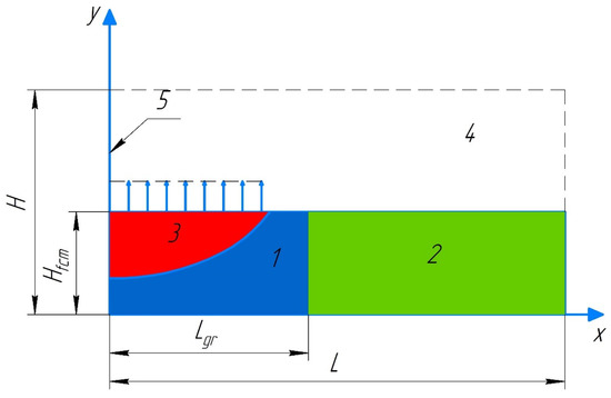
Figure 1.
Scheme of solution domain 1—wetted forest fuel; 2—dry part of forest fuel; 3—drained part of forest fuel; 4—mixture of water vapors and air; 5—forest fire front.
It was assumed in the problem statement that the main heating source of forest fuel is flame radiation. It is concentrated in the left boundary of the wetted forest fuel line (Figure 1). At t = 0, the combustion front velocity is assumed to be 0. The flame length and temperature are known and set equal to certain constant values. In practice, when a fire approaches a control line (wetted forest fuel) and the combustion front stops moving, the flame length will decrease due to the burnout of forest fuel in the region ahead of the control line. This factor was taken into account in the problem statement. The most unfavorable scenario (more complicated in terms of fire containment) was considered, in which the flame length was constant throughout the modeling time. Thus, the model values of the control line span obtained under the given conditions are bound to contain fire in more favorable situations. The flame temperature was considered constant throughout combustion duration, which was set using the experimental data [3,4].
A forest fuel layer of a given thickness Hfcm and total span L was considered (Figure 1). Some part of it was in a wetted state (the span of this part was Lgr, zone 1). The forest fuel surface is subjected to the radiant heat flux from a high-temperature source (a flame with a length Hrad and temperature Trad). As the forest fuel part wetted with water heats up, the moisture at the wet/dry interface evaporates. Then, the water vapors pass through the drained forest fuel layer (3) and are injected into the near-surface gas region (zone 4).
Based on the analysis of the experimental research [4], it was assumed that the main heat flux comes to the forest fuel surface from the flame zone as a result of radiation. In contrast, heat removal from the forest fuel surface mainly occurs due to thermogravitational convection [29], thermal conductivity of the mixture of air and water vapors and reradiation from the heated forest fuel surface. The mixture of air, water vapors and gaseous pyrolysis products is considered transparent for radiation. This approximation seems reasonable in mathematical modeling, since the introduction of the radiation absorption of the mixture would reduce the forest fuel pyrolysis rate, other things being equal.
The solution domain for the problem (Figure 1) is divided into four rectangular areas with different thermophysical characteristics: wetted forest fuel (1), dry forest fuel (2), drained forest fuel (3), gas region (4). The gas/forest fuel interface region is heated as a result of the radiant heat exchange with a high-temperature heat source (a flame with a length Hrad).
The convective–conductive heat transfer in the gas region (4) is described by the Navier–Stokes two-dimensional unsteady equations in the Boussinesq approximation (1–4) [30,31,32,33,34] and the equation of water vapor diffusion in the air (5) [33] (0 < x < L, Hfcm < y < H):
where ρ is the mixture density; µ is the dynamic viscosity of the mixture; c is the mixture heat capacity; λ is the thermal conductivity of the mixture; β is the volumetric thermal expansion coefficient of gas; g is the free-fall acceleration projected to the Y-axis (x equals 0); T0 is the initial temperature of the region; D is the water vapor diffusion coefficient in the air.
The use of a two-dimensional model in the mathematical problem statement is conditioned by the presence of a combustion front whose span is assumed by the authors to be much wider than the linear dimensions of the computational domain under study.
In numerical simulation, the density, heat capacity and thermal conductivity of the gas mixture are assumed to depend on the mass concentration of water vapors in the air:
where ca = 1005 J/(kg·K), cH2O = 4200 J/(kg·K)—heat capacity of air and water vapors; λa = 0.0259 W/(m·K), λH2O = 0.0237 W/(m·K)—thermal conductivity of air and water vapors; ρa = 1.205 kg/m3, ρp = 0.598 kg/m3—density of air and water vapors.
In the region of the wetted forest fuel (0 < x < Lgr, 0 < y < Hfcm, Figure 1), the heat transfer is given by the thermal conductivity equation in the generalized statement by Stefan [35,36]:
where c, λ, ρ—smoothed heat capacity J/(kg·K), thermal conductivity and density over the whole wetted forest fuel area: T*—boiling point (373 K); Lw—phase transition heat; ε—smoothing interval, K; cw, λw, ρw—specific isobaric heat capacity, thermal conductivity and density of wetted forest fuel; cpd, λd, ρd—specific isobaric heat capacity, thermal conductivity and density of dry forest fuel.
The heat transfer In the dry part of the forest fuel (Figure 1, region 2) (Lgr < x < L, 0 < y < Hfcm) is given by a two-dimensional unsteady equation of thermal conductivity [34,37,38]:
In region 3, the water vapors produced from the evaporation on the s(t) boundary pass through the porous frame of the dry forest fuel, cooling it down as a result of filtration. A number of assumptions were made for the mathematical description of the heat and mass transfer in the region of the drained forest fuel part: the gases are filtered at moderate rates and are assumed to be incompressible; heat transfer through thermal conductivity occurs in the porous frame (the forest fuel elements and gases have an equal temperature); local one-dimensional filtration is assumed (the vapor moves in the pores vertically upwards).
The velocity of the vapor passing through the porous frame was found, assuming the conservation of mass in the regression of the phase interface s(x,t). The average integral coordinate of the dry/wet interface of the forest fuel in the region x ϵ [0; Lgr] (average draining depth) at the point t was calculated from the following ratio:
The evaporation surface regression rate was derived from the equation:
The velocity of water vapors in the porous frame was given by
where ρwater and ρp are the densities of water and vapor.
Given the above assumptions, the energy equation under the conditions of water vapor filtration in the drained forest fuel region (Figure 1, region 3) takes the form:
where Vf is the rate of the water vapor filtration through the porous forest fuel frame; ρp is the water vapor density; cp is the heat capacity of water vapors.
The system of Equations (1)–(15) was solved with the following initial and boundary conditions:
On the boundary y = Hfcm, x ϵ [0; Lgr] (Figure 1), the concentration of water vapors and the vertical component of their velocity were set:
It was assumed that the resultant heat flux qri comes to the gas/forest fuel interface (y = Hfcm, 0 ≤ x ≤ L) from the source with a length Hrad (flame) with a constant temperature Trad. The value of qri on the forest fuel surface was determined using the zonal method [37,39]. In the case of an isothermal surface with a length Hrad, the resultant heat flux equals [37]:
where E0i and E0k are the total radiant fluxes per unit area of a black body of the i-th and k-th surfaces, W/m2; Ai = 1 and Ak = 0.97 are the emissivities of the i-th and k-th surfaces; φi,k are local angular coefficients (depending only on the body system geometry).
When the elemental areas are perpendicular (Figure 2) (there is no wind), the angular coefficients were given by [40,41]
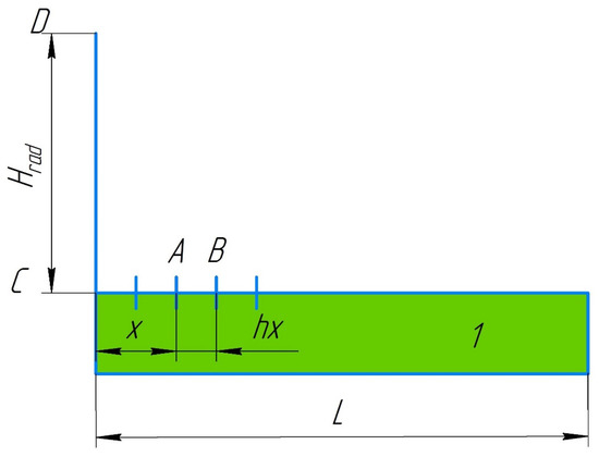
Figure 2.
Scheme of radiant heat flux calculation.
When the geometrical layout of the bodies was as presented in Figure 2, the areas of the elements participating in the radiant heat exchange were calculated using the equations:
where x ϵ [0; L] is the forest fuel surface coordinate; l is the linear size in the direction perpendicular to the X0Y plane; hx is a step on the forest fuel surface in the X-axis direction.
Given the resultant radiant flux, the boundary condition on the ‘mixture of the air and water vapors/forest fuel’ interface takes the form:
The mathematical model is represented by a system of differential equations with initial and boundary conditions (16)–(36). The finite volume method was used as a discretization method for all the equations. In this method, the computational domain is partitioned into a finite set of disjoint control volumes that contain one node point. After that, the initial differential equation is integrated over each control volume, assuming the profile of the function change between the nodes to be a known value. In this manuscript, the power law differencing scheme of the unknown value between the nodes of the computational mesh was applied for each differential equation. The time approximation was performed using the fully implicit scheme [40,41].
The equations include the value of pressure for the projection of the momentum. To find the pressure field, the SIMPLE algorithm was utilized [42]. This is an iterative algorithm. It calculates the pressure field satisfying the momentum equation in line with continuity conservation. The algorithm requires that a staggered grid be used.
Each differential equation is converted to a six-point discrete analog (using the above described finite volume method). The alternating direction method works well when solving such kind of algebraic equation systems. It suggests applying the Thompson’s algorithm along each grid line. The algorithm is repeated until the system is solved with the required accuracy.
The connection between the domains is determined by the conditions specified at inner and outer boundaries, i.e., when solving the differential equation system, the obtained fields satisfy the discrete analogs of differential equations and the specified boundary conditions.
Differential equations are solved in sequence, while the system is solved iteratively. At each time step, all the algebraic equation systems are solved until a convergent solution is obtained with the prescribed accuracy for all the unknown values. The code was written by the authors in Delphi.
3. Results and Discussion
The calculations were performed with the computational domain dimensions H × L = 0.1 × 1 m2 and flame length of 0.15 m. The radiation source temperature was taken to be 900 K. This ensured that the average heat flux to the forest fuel surface was close to the one obtained experimentally [3]. Moreover, based on the experimental research findings obtained under laboratory conditions [27], as assumption was made that the time of the complete burnout of forest fuels when using a wet line ahead of the combustion front was 120 s. The typical wet line width in the experiments [3] was no more than 0.5 m with a material sample thickness up to 0.05 m. Therefore, the mathematical modeling results in Figure 3 are shown at a point t = 120 s at a control line span Lgr of 0.3 m. The thickness of a coniferous forest fuel sample Hfcm was 0.05 m. These conditions can be considered general for different values of the radiant heat flux and flame length when analyzing the typical fire suppression conditions. By analyzing the mathematical modeling results under these conditions and taking account of the experimental data on fire types, characteristics and sizes [3,4,27], it is possible to predict how far the flame length affects the containment time and liquid consumption volume when using different component compositions. The experiments [3,4,27] compare the integral characteristics of forest fuel combustion when using liquids without additives, slurries, emulsions and solutions.
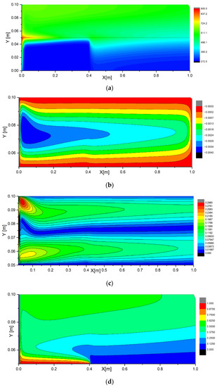
Figure 3.
Temperature distribution (a) (K) in the forest fuel layer and in gas; contour lines of the stream function (b) (m2/s) of the mixture of air and water vapors near the forest fuel surface; contour lines of the velocity vector module (c) (m/s) near the forest fuel surface; mass concentration of water vapors in the air near the forest fuel surface (d).
The analysis of the numerical simulation results established that a wet line has a significant influence on the heat transfer characteristics (Figure 3a). The moisture in the pores of forest fuel slows down its heating due to the absorption of heat during the phase transition and therefore the higher heat capacity c of the wet forest fuel compared to the dry one. As a result, the wetted forest fuel part is heated much more slowly than the dry one is. Moreover, the injection of relatively cold water vapors that have passed through the porous frame of the drained forest fuel part reduces the temperature of the forest fuel surface and the gas mixture around it. The dry part of the forest fuel (y = 0.05 m; 0.3 ≤ x ≤ 1 m) subjected to the resultant radiant heat flux and natural convective heat exchange heated up much faster and had a higher maximum surface temperature (approx. 471 K). At the same time, the temperature profiles were highly nonlinear, which indicates that the heating rates of the material were different in the deep and near-surface layers of the sample. These profiles also illustrate the heat transfer directions and temperature fluctuations. The analysis of T (x, y) distributions at different points in time indicates the conditions of the most efficient suppression of forest fires. Thus, it is possible to predict the minimum volume of moisture in a forest fuel sample necessary to contain combustion of varying intensities and pyrolyzing material thickness.
Figure 3b,c show the contour lines of the stream function and the gas mixture velocity vector near the forest fuel surface (0 ≤ x ≤ L; 0.05 ≤ y ≤ 0.1). It is clear that the nonuniform heating of the material surface results in a whirl with vertical movement along the boundary y = 0. The negative values of the contour line of the current function are typical of the clockwise movement. Figure 3c shows the contour lines of the velocity vector module of the gas mixture near the forest fuel surface. Uneven heating of the forest fuel surface due to the radiant flux from a high-temperature source intensifies natural convection in the gas region. A vortex with vertical movement along the boundary x = 0 forms by the time point considered in the study. The above described convective processes have a direct effect on the temperature field generation and development near the forest fuel surface, as well as on the temperature distribution over it within the whole time interval of the problem solution. The maximum values of the velocity vector module were 0.290 m/s in the fairly typical conditions under consideration.
The flame radiation heats the surface of the dry forest fuel too (contour lines in Figure 3a). This heating then initiates and maintains the swirling of the air/water vapor mixture (Figure 3b,c). The calculation results for the water vapor concentrations are shown in Figure 3d. Due to a vapor flow injected into the near-wall area, thermogravitational convection and water vapor diffusion in the air, the mass concentration distribution of the water vapor is highly inhomogeneous. When moving away from the forest fuel surface, the water vapor concentration grows in the region above the dry part of the forest fuel and falls in the region above its wetted part.
Figure 4 presents the forest fuel surface temperatures (T) at varying control line spans (Lgr = 0.2; 0.3; 0.4 m), other things being equal. It is clear that an increase in the control line span leads to a lower maximum temperature of the forest fuel surface (its unwetted part). It is apparent from Figure 4 that the T(x) curve is quite complex.
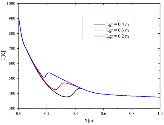
Figure 4.
Forest fuel surface temperature at different control line spans.
The distributions of the forest fuel surface temperature on the coordinate parallel to this surface, presented in Figure 4, can be tentatively divided into three regions corresponding to certain variations of the temperature T.
The first one—500 K ≤ T ≤ 900 K (for Lgr = 0.2 m)—corresponds to the span of the control line from which all the moisture has already evaporated. A great temperature variation over the surface of this region illustrates the distributed flows from the combustion front, on the one hand, and the effect of water and water vapors, on the other hand. Farther away from the combustion front, the forest fuel surface temperature quickly decreases due to the moisture evaporating in the control line structure. The local minima and maxima on the three curves T(x) at different spans of control lines illustrate the second characteristic region that includes a small area to the left of the right boundary of the control line and to the right of this boundary. The local maxima of the surface temperature on the curves in Figure 4 correspond to a small area behind the control line on the right, where water and its vapors have a modest effect. The third area of T(x) is characterized by a slight rise in the temperature of the forest fuel surface due to radiant heating from the flame front that is quite far from the forest fuel.
When determining the effective value of the control line span (at which forest fuel combustion stops), it was assumed that the thermal decomposition begins at a temperature of 473 K. If the maximum temperature of the forest fuel surface does not reach the pyrolysis initiation temperature during the numerical experiment (120 s), the thermal decomposition completely stops and the forest fuel combustion is contained. Figure 4 shows the curve of the maximum temperature of the forest fuel surface versus the wet line span. At a flame length Hrad of 0.15 m, the minimum span of the control line Lgr, at which combustion is contained, is 0.3 m.
The key parameter to be defined when preparing a control line is its span in the direction of the surface fire spread (the line width) at a flame height characteristic of particular terrain and type of forest fuel. Significantly, control lines of wetted forest fuels are effective in fighting surface fires whose initial stage is characterized by relatively low flame heights (under 1 m). The combustion temperature of wood of different types ranges from 300 to 1100 K.
The experiments [27] revealed that the minimum effective span of the wet line ahead of the flame front for coniferous forest fuel with a sample thickness of 0.05 m was 0.3 m. This indicates that the modeling results are consistent with the experimental data from [27]. The minimum wet line span in the mathematical model above is 40% higher than the experimental value and is 0.5 m (Figure 5). This difference in the effective values of Lgr can be attributed to the fact that the flame length during the numerical experiment was taken to be constant. In a real fire, the flame length ahead of the wet line decreases over time (which was recorded in the experiments [27]). This process reduces the heat flux to the forest fuel surface, and the fire suppression condition is satisfied at lower Lgr.
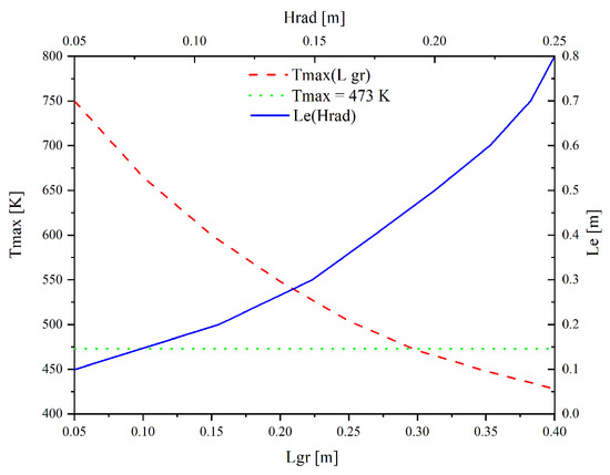
Figure 5.
Maximum forest fuel surface temperature depending on the control line span and the effective control line span (typical size of the wetted forest material strip ahead of the combustion front) at different flame lengths.
Figure 5 presents the effective span (Le, characteristic width) of the wet line, which should be placed ahead of the combustion front using hand tools or an aircraft, calculated for varying flame lengths. The effective wet line span increases with an increase in the flame length. In a real fire, the higher the flame, the greater the heat flux supplied to the forest fuel surface and the higher the vaporization rates. This process results in a buffer vapor layer emerging between the forest fuel and the flame zone. As a result, the rates of the physical and chemical processes decrease, which stabilizes the forest fuel surface temperature to some degree.
The experience of combatting forest fires on all the populated continents over the last 5–10 years demonstrates that the efforts to completely suppress fire on a large area are not very effective (it is impossible to provide large amounts of water or specialized firefighting agents due to a limited number of airtankers) [12]. It appears to be more effective to fight forest fires by containing them and preventing the combustion spread beyond the boundaries of certain fire areas. In this respect, two recommendations on the practical application of control lines in surface fire containment follow from the fire suppression characteristics (primarily temperature), obtained in this numerical study. The first one is that the control line span should be chosen from the comparison of the heat spent on complete evaporation of all the water accumulated by the control line with the heat content of the bulk of the flame advancing towards this line.
The numerical analysis revealed that with a layer of forest fuel fairly typical thickness (0.05 m), its surface temperature does not rise to the temperature of rapid thermal decomposition until all the moisture accumulated in it evaporates. Water vapors leaking to the heating surface of forest fuel cool the elements of its structure (needles, leaves, twigs). Moreover, the heat capacity of water vapors is quite high, and the heat reaching the forest fuel surface is partially absorbed by them. Significantly, the water vapors entering the air layer near the heated surface of forest fuel, when continuing their movement through the radiation flux to the forest fuel surface, reduce the concentration of combustible gases ahead of the flame front, slowing down combustion. The mass concentrations of water vapors in the air near the forest fuel surface, presented in Figure 3d, illustrate the above conclusions.
When water is sprayed from an aircraft immediately above the flame, most of the water droplet flow was found [3] to pass through the flame and reach a layer of forest fuel that had already burned out, having no far-reaching effect on fire suppression or containment. There is no point in cooling the forest fuel layer in which pyrolysis, generating combustible gases, almost stopped. Moreover, pyrolysis significantly increases the volume of pores in the forest fuel structure, and water droplets pass through this highly porous structure, reaching the boundary separating forest fuel and soil. This makes water application ineffective. If water arrives on the control line of forest fuel in the initial state, water droplets wet the forest fuel structure elements (e.g., needles). Further heating causes this moisture to evaporate completely.
Another recommendation arises from these findings: it is a good idea to compact a forest fuel layer before wetting it, if possible; this would minimize the trickling of water off the pores of highly porous forest fuel to the ‘forest fuel–soil’ interface.
4. Conclusions
The results of the numerical studies on the thermophysical processes and fluid dynamics in the area of a control line constructed of wetted forest fuel indicate that the proposed approach to the mathematical modeling of heat transfer in the ‘forest fuel–control line’ system makes it possible to adequately describe the conditions and characteristics of forest fire containment when forest fuel is wetted ahead of the fire front. The influence of the flame length (being the main factor determining forest fuel heating intensity) in a forest fire (impossible to reproduce in laboratory experiments) can be reliably estimated using the mathematical model developed in this study.
Author Contributions
G.K.—conceptualization, funding acquisition; A.K.—software and validation; A.Z.—Writing—Original draft preparation of manuscript. All authors have read and agreed to the published version of the manuscript.
Funding
The Research was supported by the Russian Science Foundation (project No 21-19-00009, https://rscf.ru/en/project/21-19-00009/).
Conflicts of Interest
The authors declare no conflict of interest.
References
- Thompson, M.P.; Calkin, D.E.; Herynk, J.; McHugh, C.W.; Short, K.C. Airtankers and wildfire management in the US Forest Service: Examining data availability and exploring usage and cost trends. Int. J. Wildl. Fire 2013, 22, 223–233. [Google Scholar] [CrossRef]
- Vysokomornaya, O.V.; Kuznetsov, G.V.; Strizhak, P.A. Experimental investigation of atomized water droplet initial parameters influence on evaporation intensity in flaming combustion zone. Fire Saf. J. 2014, 70, 61–70. [Google Scholar] [CrossRef]
- Volkov, R.S.; Kuznetzov, G.V.; Strizhak, P.A. Experimental Determination of the Fire Break Size and Specific Water Consumption for Effective Control and Complete Suppression of the Front Propagation of a Typical Ground Fire. Appl. Mech. Tech. Phys. 2019, 60, 79–93. [Google Scholar] [CrossRef]
- Atroshenkom, Y.K.; Kuznetsov, G.V.; Strizhak, P.A.; Volkov, R.S. Protective Lines for Suppressing the Combustion Front of Forest Fuels: Experimental Research. Process Saf. Environ. Prot. 2019, 13, 73–88. [Google Scholar] [CrossRef]
- Li, X.; Zhang, M.; Zhang, S.; Liu, J.; Sun, S.; Hu, T.; Sun, L. Simulating Forest Fire Spread with Cellular Automation Driven by a LSTM Based Speed Model. Fire 2022, 5, 13. [Google Scholar] [CrossRef]
- Jiang, W.; Wang, F.; Su, G.; Li, X.; Wang, G.; Zheng, X.; Wang, T.; Meng, Q. Modeling Wildfire Spread with an Irregular Graph Network. Fire 2022, 5, 185. [Google Scholar] [CrossRef]
- Edalati-Nejad, A.; Ghodrat, M.; Fanaee, S.A.; Simeoni, A. Numerical Simulation of the Effect of Fire Intensity on Wind Driven Surface Fire and Its Impact on an Idealized Building. Fire 2022, 5, 17. [Google Scholar] [CrossRef]
- Anand, C.; Shotorban, B.; Mahalingam, S.; McAllister, S.; Weise, D.R. Physics-based modeling of live wildland fuel ignition experiments in the forced ignition and flame spread test apparatus. Combust. Sci. Technol. 2017, 189, 1551–1570. [Google Scholar] [CrossRef]
- Fuentes, A.; Consalvi, J.L. Experimental study of the burning rate of small-scale forest fuel layers. Int. J. Therm. Sci. 2013, 74, 119–125. [Google Scholar] [CrossRef]
- Bebieva, Y.; Speer, K.; White, L.; Smith, R.; Mayans, G.; Quaife, B. Wind in a natural and artificial wildland fire fuel bed. Fire 2021, 4, 30. [Google Scholar] [CrossRef]
- Fateev, V.; Agafontsev, M.; Volkov, S.; Filkov, A. Determination of smoldering time and thermal characteristics of firebrands under laboratory conditions. Fire Saf. J. 2017, 91, 791–799. [Google Scholar] [CrossRef]
- Zhdanova, A.; Volkov, R.; Voytkov, I.; Osipov, K.; Kuznetsov, G. Suppression of forest fuel thermolysis by water mist. Int. J. Heat Mass Transf. 2018, 126, 703–714. [Google Scholar] [CrossRef]
- Johnston, J.M.; Wheatley, M.J.; Wooster, M.J.; Paugam, R.; Davies, G.M.; DeBoer, K.A. Flame-front rate of spread estimates for moderate scale experimental fires are strongly influenced by measurement approach. Fire 2018, 1, 16. [Google Scholar] [CrossRef]
- Hoffman, C.M.; Sieg, C.H.; Linn, R.R.; Mell, W.; Parsons, R.A.; Ziegler, J.P.; Hiers, J.K. Advancing the science of wildland fire dynamics using process-based models. Fire 2018, 1, 32. [Google Scholar] [CrossRef]
- Marshall, G.; Thompson, D.K.; Anderson, K.; Simpson, B.; Linn, R.; Schroeder, D. The Impact of Fuel Treatments on Wildfire Behavior in North American Boreal Fuels: A simulation Study Using FIRETEC. Fire 2020, 3, 18. [Google Scholar] [CrossRef]
- De Silva, D.; Sassi, S.; De Rosa, G.; Corbella, G.; Nigro, E. Effect of the Fire Modelling on the Structural Temperature Evolution Using Advanced Calculation Models. Fire 2023, 6, 91. [Google Scholar] [CrossRef]
- Zhao, J.; Wang, Z.; Hu, Z.; Cui, X.; Peng, X.; Zhang, J. Effects of Fire Location and Forced Air Volume on Fire Development for Single-Ended Tunnel Fire with Forced Ventilation. Fire 2023, 6, 111. [Google Scholar] [CrossRef]
- Grishin, A.M.; Shipulina, O.V. Mathematical model for spread of crown fires in homogeneous forests and along openings. Combust. Explos. Shock Waves. 2002, 38, 622–632. [Google Scholar] [CrossRef]
- Subbotin, A.N. Mathematical model of ground fire spread over forest litter and fallen conifer needles. Fire Saf. J. 2008, 1, 109–116. [Google Scholar]
- Kopylov, N.P.; Kopylov, N.P.; Khasanov, I.R.; Kuznetsov, A.E.; Fedotkin, D.V.; Moskvilin, E.A.; Strizhak, P.A.; Karpov, V.N. Aerial water drop parameters for forest fire suppression. Fire Saf. J. 2015, 2, 49–55. [Google Scholar]
- Grishin, A.M.; Zima, V.P.; Kuznetsov, V.T.; Skorik, A.I. Ignition of combustible forest materials by a radiant energy flux. Combust. Explos. Shock Waves. 2002, 38, 24–29. [Google Scholar] [CrossRef]
- Snegirev, A.Y.; Tsoy, A.S. Treatment of local extinction in CFD fire modeling. Proc. Combust. Inst. 2015, 35, 2519–2526. [Google Scholar] [CrossRef]
- Korobeinichev, O.P.; Shmakov, A.; Chernov, A.A.; Bol’Shova, T.A.; Shvartsberg, V.M.; Kutsenogii, K.P.; Makarov, V.I. Fire suppression by aerosols of aqueous solutions of salts. Combust. Explos. Shock Waves 2010, 46, 16–20. [Google Scholar] [CrossRef]
- Korobeinichev, O.P.; Paletsky, A.A.; Gonchikzhapov, M.B.; Shundrina, I.K.; Chen, H.; Liu, N. Combustion chemistry and decomposition kinetics of forest fuels. Procedia Eng. 2013, 62, 182–193. [Google Scholar] [CrossRef]
- Korobeinichev, O.; Shmakov, A.; Shvartsberg, V.; Chernov, A.; Yakimov, S.; Koutsenogii, K.; Makarov, V. Fire suppression by low-volatile chemically active fire suppressants using aerosol technology. Fire Saf. J. 2012, 51, 102–109. [Google Scholar] [CrossRef]
- Kataeva, L.Y.; Maslennikov, D.A. Influence of the water barrier on the dynamics of a forest fire considering the inhomogeneous terrain and two-tier structure of the forest. ARPN J. Eng. Appl. Sci. 2016, 11, 2972–2980. [Google Scholar]
- Kataeva, L.Y.; Maslennikov, D.A.; Loshchilova, N.A. On the laws of combustion wave suppression by free water in a homogeneous porous layer of organic combustible materials. Fluid Dyn. 2016, 51, 389–399. [Google Scholar] [CrossRef]
- Beer, T. The interaction of wind and fire. Bound. -Layer Meteorol. 1991, 54, 287–308. [Google Scholar] [CrossRef]
- Finney, M.A.; Cohen, J.D.; Forthofer, J.M.; McAllister, S.S.; Gollner, M.J.; Gorham, D.J.; Saito, K.; Akafuah, N.K.; Adam, B.A.; English, J.D. Role of buoyant flame dynamics in wildfire spread. Proc. Natl. Acad. Sci. USA 2016, 112, 9833–9838. [Google Scholar] [CrossRef]
- Schlichting, H. Boundary Layer Theory; Nauka: Moscow, Russia, 1974. [Google Scholar]
- Anderson, D.; Tannehill, D.; Pletcher, R. Basic equations of fluid mechanics and heat transfer. In Computational Fluid Dynamics and Heat Transfer; Mir: Moscow, Russia, 1990; Volume 1. [Google Scholar]
- Anderson, D.; Tannehill, D.; Pletcher, R. Numerical methods for solving the Navier–Stokes equations. In Computational Fluid Dynamics and Heat Transfer; Mir: Moscow, Russia, 1990; Volume 2. [Google Scholar]
- Poinsot, T.; Veynante, D. Theoretical and Numerical Combustion; Erdwards: Eagle County, CO, USA, 2001. [Google Scholar]
- Incopera, F.P.; DeWitt, D.P. Fundamentals of Heat Transfer and Mass Transfer, 5th ed.; John Wiley & Sons: New York, NY, USA, 2002. [Google Scholar]
- Samarskii, A.A.; Vabishchevich, P.N. Computational Heat Transfer; Editorial URSS: Moscow, Russia, 1987. [Google Scholar]
- Vabishchevich, P.N. Numerical Methods of Solving Free-Boundary Problems; MSU Press: Moscow, Russia, 1987. [Google Scholar]
- Isachenko, V.P.; Osipova, V.A.; Sukomel, A.S. Heat Transfer, 3rd ed.; Energiya: Moscow, Russia, 1975. [Google Scholar]
- Drysdale, D. An Introduction to Fire Dynamics, 2nd ed.; John Wiley & Sons: New York, NY, USA, 1998. [Google Scholar]
- Siegel, R.; Howell, J. Thermal Radiation Heat Transfer; Mir: Moscow, Russia, 1975. [Google Scholar]
- Patankar, S. Numerical Heat Transfer and Fluid Flow; Energoatomizdat: Moscow, Russia, 1984. [Google Scholar]
- Paskonov, V.M.; Polezhaev, V.I.; Chudov, L.A. Numerical Simulation of Heat and Mass Transfer; Nauka: Moscow, Russia, 1984. [Google Scholar]
- Versteeg, H.G.; Malalasekera, W. An Introduction to Computational Fluid Dynamics; Pearson Education Limited: Harlow, UK, 2007. [Google Scholar]


Disclaimer/Publisher’s Note: The statements, opinions and data contained in all publications are solely those of the individual author(s) and contributor(s) and not of MDPI and/or the editor(s). MDPI and/or the editor(s) disclaim responsibility for any injury to people or property resulting from any ideas, methods, instructions or products referred to in the content. |
© 2023 by the authors. Licensee MDPI, Basel, Switzerland. This article is an open access article distributed under the terms and conditions of the Creative Commons Attribution (CC BY) license (https://creativecommons.org/licenses/by/4.0/).