Study on the Prediction Model of Coal Spontaneous Combustion Limit Parameters and Its Application

Abstract

The limit parameters of coal spontaneous combustion are important indicators for determining the risk of spontaneous combustion in coal seams. By analyzing the limit parameters of coal spontaneous combustion, the dangerous areas of coal spontaneous combustion can be determined, and corresponding measures can be taken to avoid the occurrence of fires. In order to accurately predict the limit parameters of coal spontaneous combustion, the prediction model of coal spontaneous combustion limit parameters based on GA-SVM was constructed by coupling genetic algorithm (GA) and support vector machine (SVM). Meanwhile, the GA and particle swarm optimization algorithm (PSO) were used to optimize the back propagation neural network (BPNN) to construct the GA-BPNN and PSO-BPNN prediction models, respectively. To predict the intensity of air leakage of the upper limit of coal spontaneous combustion in the goaf, the prediction results of the models were compared and analyzed using MAE, MAPE, RMSE, and R² as the prediction performance evaluation indexes. The results show that the MAE of the GA-SVM model, the PSO-BPNN model, and the GA-BPNN model are 0.0960, 0.1086, and 0.1309, respectively; the MAPE is 2.46%, 3.11%, and 3.69%, respectively; the RMSE is 0.1180, 0.1789, and 0.2212, respectively; and the R² is 0.9921, 0.9818, and 0.9722. The prediction results of the GA-SVM model are the most optimal in four evaluation indexes, followed by the PSO-BPNN and the GA-BPNN models. Applying each model to the prediction of minimum residual coal thickness in the goaf of a coal mine in Shanxi, the GA-SVM model has higher accuracy, which further verifies the universality and stability of the model and its suitability for the prediction of coal spontaneous combustion limit parameters.

1. Introduction

Coal spontaneous combustion is a coal mine endogenous fire affected by multiple factors. Such fires constitute a large proportion of mine fires and seriously restrict the high productivity, high efficiency, and safe production of mines [1,2]. Since the spontaneous combustion of coal requires meeting certain conditions, the quantitative indicators are applied to describe the coal spontaneous combustion conditions [3]. When the oxidized exothermicity of coal itself is equal to the heat dissipation intensity of the surrounding environment, it may cause spontaneous combustion of coal, which is the limiting condition for triggering spontaneous combustion of coal, also known as the limiting parameter of coal spontaneous combustion [4,5], mainly including the lower limit oxygen concentration, the upper limit air leakage intensity, and the minimum floating coal thickness [6]. Due to the complicated influencing factors of coal spontaneous combustion limit parameters, the relationship between the limit parameters and the influencing factors is characterized by nonlinearity. Therefore, scientific and effective methods are used to predict the limit parameters of the spontaneous combustion of coal, and, then, accurately determine the dangerous zone of the occurrence of spontaneous combustion of coal, which has important significance for coal mine fire prevention and suppression work.

In recent years, related scholars have carried out much research around coal spontaneous combustion limit parameters [7,8]. Xu Jingcai et al. [9] studied the relationship between the spontaneous combustion limit parameters of coal and their influencing factors, and proposed to predict the spontaneous combustion limit parameters of coal by using a BP neural network. Deng Jun et al. [10] studied the exothermicity and oxygen consumption rate of coal samples from mines in the east Sichuan region on the basis of programmed heating experiments, and analyzed the gas products of each coal sample at different temperatures as well as the change rule of the spontaneous combustion limit parameters. Meng Qian et al. [11] applied the support vector machine to the prediction of the spontaneous combustion limit parameters of coal and made contrastive analysis with the neural network model, which can result in a high prediction accuracy with a limited number of samples. Wang C et al. [12] made contrastive analysis for the spontaneous combustion limit parameters of coal with different degrees of metamorphism through the spontaneous combustion programmed heating experiment, and concluded the change rule of the limit parameters. Zhang Y et al. [13] studied the effect of sulfur content in coal on the spontaneous combustion characteristics and the limiting parameters of coal. Zhang Fei [14] analyzed the spontaneous combustion and characteristics of oxidation and the limit parameters of No. 4 seam coal in the Xiagou mine with the help of the coal spontaneous combustion programmed heating experiment, and diagnosed the spontaneous combustion hazardous area of the coal left at a work face in the upper and lower goaf during the final mining period. Wang Yilei et al. [15] tested coal samples from a high geothermal mine by a large coal spontaneous combustion experimental device to determine the coal spontaneous combustion limiting parameters, and the natural combustion period as well as the generation rules of oxidization-characteristic gases in high geothermal mines at different temperatures. Zhang Xinhai et al. [16] calculated coal spontaneous combustion limiting parameters by the analytical solution method, which was verified by practical application in the Kaida coal mine. Wang Jianli et al. [17] studied the effect of sulfur content in coal on the spontaneous combustion characteristics and the limiting parameters of coal. Zhou Xihua et al. [18] investigated the changes of lignite spontaneous combustion limiting parameters under different air supply conditions by analysing the temperature programmed experiments. However, the above studies mainly focused on analysis and verification of the coal spontaneous combustion limiting parameters through experimental tests or single prediction models, while few scholars conducted studies utilising combined prediction models. In order to reduce the errors by simplified calculation and avoid the defects of the single prediction model because of the complexity of the influencing factors of coal spontaneous combustion limiting parameters, it is necessary to establish the prediction model of coal spontaneous combustion limiting parameters by combining machine learning methods to improve prediction accuracy, which could provide better guidance for the prevention and control of coal spontaneous combustion in the goaf.

In view of this, based on the analysis of the influencing factors of coal spontaneous combustion limit parameters by the previous authors, the author intends to combine the genetic algorithm (GA) and use of the support vector machine (SVM) into the prediction of coal spontaneous combustion limit parameters to construct a GA-SVM prediction model. In order to verify the accuracy of the prediction model, the GA and particle swarm optimization (PSO) algorithms were used to improve the BP neural network to establish the GA-BPNN model and PSO-BPNN model, respectively. These models were applied to the prediction of coal spontaneous combustion limit parameters in a coal mine in Shanxi to get a better prediction model by analyzing these prediction results, with a view to providing a theoretical basis for the prevention and management of the natural ignition of coal.

2. Optimized BP Neural Network Model

2.1. Sample Data

Taking the upper limit air leakage intensity of coal spontaneous combustion limit parameters as an example, the prediction model of coal spontaneous combustion limit parameters was constructed. There are five parameters in the input layer in the prediction model, namely, exothermic strength, coal body temperature, measured oxygen volume fraction, distance of the goaf from the working face, and thickness of the remaining coal; the output layer is the upper limit air leakage strength. The data from the reference [9] are selected as samples for prediction, the training samples are shown in

Table 1. Training sample data.

No.	Distance/m	Oxygen Concentration/%	Coal Temperature/°C	Heat Liberation Intensity/105 J·s−1·cm−3	Thickness of Residual Coal/m	Upper Limit Air Leakage Intensity/cm3·cm−2·s−1
1	1.7	20.60	19.60	0.87	0.7	0.70
2	2.5	20.04	20.30	1.04	0.6	0.83
3	4.7	19.88	22.00	1.27	0.5	1.08
4	7.6	19.03	22.50	1.34	0.4	1.56
5	16.3	18.21	24.20	1.43	0.2	2.35
6	20.5	17.99	25.60	1.51	0.3	2.58
7	25.2	17.60	26.70	1.58	0.4	2.88
8	29.1	17.36	26.80	1.58	0.3	3.17
9	36.4	16.90	27.50	1.62	0.2	3.43
10	43.9	15.74	28.30	1.67	0.3	3.87
11	44.3	15.68	28.60	1.69	0.4	3.92
12	47.0	14.91	28.10	1.66	0.5	4.12
13	53.7	13.77	25.13	1.49	0.7	5.60
14	56.4	13.09	24.80	1.47	0.6	5.77
15	59.0	12.44	24.30	1.43	0.5	6.00
16	61.2	11.93	23.60	1.40	0.4	6.53
17	70.6	10.78	24.67	1.46	0.2	5.39
18	74.3	9.81	26.30	1.55	0.2	4.18
19	78.0	8.85	27.80	1.61	0.3	3.76
20	89.2	7.14	30.40	1.79	0.3	2.89

, and the test samples are shown in

Table 2. Test sample data.

No.	Distance/m	Oxygen Concentration/%	Coal Temperature/°C	Heat Liberation Intensity/105 J·s−1·cm−3	Thickness of Residual Coal/m	Upper Limit Air Leakage Intensity/cm3·cm−2·s−1
21	11.0	18.59	23.40	1.39	0.3	1.88
22	39.7	16.50	27.90	1.64	0.2	3.52
23	50.4	14.36	28.20	1.66	0.6	4.24
24	66.8	11.18	24.20	1.43	0.3	6.01
25	83.5	7.97	28.10	1.66	0.4	3.76

.

2.2. BP Neural Network

The BP neural network is one of the most widely used methods in artificial neural network models and algorithms. The BP neural network is a feed-forward multi-layer neural network with the main features being back propagation of the error and transmission forward of the signal [19]. The main idea of the BP neural network algorithm is to import the original sample data into the BP neural network prediction model, then the actual output of the BP neural network is obtained through arithmetic. When the relative error between the actual output and the desired output does not meet the requirements of the error accuracy, the error is propagated in the reverse direction to promptly adjust the weights and thresholds in the BP neural network model. Then, the original sample data are reintroduced for another calculation, which could reduce the relative errors between the actual output and the desired output to meet the requirements of error accuracy.

The BP neural network model consists of three parts, namely, input layer, hidden layer, and output layer. The mathematical expression is the following:

$$h_j=f(x_j)=\frac{1}{1+\exp (-{\displaystyle {\sum }_{j=1}^p{l}_j}{b}_j+\epsilon )},j=1,2,\dots ,p$$

(1)

where h_j is the output value, f(x) is the activation function, x_j is the input value, l_j is the connection weights of the hidden nodes, b_j is the threshold between the hidden nodes, ε is the threshold of the hidden nodes, and p is the number of hidden nodes.

A coal spontaneous combustion limit parameters prediction model was constructed based on the BP neural network in the reference [9], but the BP neural network has some defects of non-convergence, slow convergence, and output results that easily fall into the local minima during the training process. In order to predict the coal spontaneous combustion limit parameters more accurately and avoid the shortcomings of the BP neural network, the GA and PSO, respectively, are introduced to optimize the BP neural network.

2.3. GA-BP Neural Network Model

The genetic algorithm (GA) is a parallel and random search optimization algorithm which simulates the genetic mechanism of nature and biological evolution. Based on the principles of selection, crossover, and mutation of genetics, the initial weights and thresholds of BP neural networks are improved by the GA so that the optimized BP neural network can better predict the output values. The elements of the BP neural network optimized by GA include cluster initialization, fitness function, selection operation, crossover operation, and mutation operation [20,21]. The genetic algorithm mainly has the following steps:

(1)

Coding. Real coding is used to prevent falling into the local optimum with the mean square error as the evaluation index and the inverse of the mean square error 1/EMSE as the fitness function f. The smaller the loss is, the higher the fitness is, i.e.,

$$f=1/E_{MSE}=1/\left(\frac{1}{N}{\displaystyle \sum {\left(O-T\right)}^2}\right)$$

(2)

where O is the model desired output, T is the mean, and N is the number of input samples.

(2)

Generating initial population. N individuals that are randomly generated form a population. The GA starts evolving continuously based on the initial point.

(3)

Selecting operator. The purpose of the selection operation is to pick the best individuals which can reproduce their offspring as parents, reflecting the idea of survival of the fittest. The probability of individual selection is based on a method of roulette wheel, that is, individuals that account for a larger proportion of fitness have a higher chance of being selected.

$$P_k=f_k/{\displaystyle \sum _{j=1}^N{f}_i}$$

(3)

where k represents individuals in the population.

(4)

Crossover operator. Crossover operation is a major genetic method of genetic algorithm, reflecting the idea of information exchange. The real coding method is adopted in this paper. The method of crossover is to take a (0, 1) random number m and a certain position (j) in the two chromosomes (a_k and a_l) for crossover, combining to get two new chromosomes, i.e.,

$$\{\begin{array}{c}{a}_{kj}^{\prime }=a_{kj}(1-m)+a_{lj}m\\ a_{lj}^{\prime }=a_{lj}(1-m)+a_{kj}m\end{array}$$

(4)

(5)

Mutation operator. Mutation is the process of mutating selected individuals to form new individuals on the basis of a particular probability, which is to maintain the diversity of the population. Based on the random probability r (r $\in$ (0, 1)), the yth gene of the xth chromosome is selected to mutate and the mutated chromosome a′_xy is obtained with the expression:

$$a_{xy}^{\prime }=\{\begin{array}{cc}{a}_{xy}+\left(a_{xy}-a_{max}\right)f\left(t\right)& r>0.5\\ a_{xy}+\left(a_{min}-a_{xy}\right)f\left(t\right)& r\le 0.5\end{array}$$

(5)

where a_max and a_min are the upper and lower bounds of gene a_xy, respectively, and f(t) = r₁(1 − t/G_max), where t is the current iteration number, G_max is the maximum evolution number, and r₁ is a random number of (0, 1).

The GA-BPNN prediction model was constructed by utilising the MATLAB R2021b software, setting the number of neurons in the hidden layer to 20, the number of genetic generations to 50, the population to 5, the maximum number of iterations to 1000, the learning rate to 0.01, and the error threshold to 0.0000001. The specific parameter settings are shown in

Table 3. Parameter setting of the GA-BPNN model.

Parameter	Specific Values
Genetic generations	50
Population size	5
Maximum number of iterations	1000
Learning rate	0.01
Error threshold	0.0000001

. The iteration process of the GA-BP neural network is shown in Figure 1, and when the number of iterations reaches 100, the fitting rate reaches 0.9422. The results from the GA-BPNN prediction model are shown in

Table 4. Comparison between real values and predicted values of the GA-BPNN model.

No.	True Values /cm3·cm−2·s−1	Prediction Values /cm3·cm−2·s−1	Absolute Error	Relative Error/%
1	1.88	1.9433	0.0633	3.37
2	3.52	3.5554	0.0354	1.00
3	4.24	4.2388	0.0012	0.03
4	6.01	5.9394	0.0706	1.17
5	3.76	4.2442	0.4842	12.88

. As can be seen from Table 4, the relative error between the predicted and true values of the GA-BPNN modeling operations ranged from 0.03% to 12.88%, with a difference of 12.85% and an average relative error of 3.69%, while the absolute error ranged from 0.0012 to 0.4842, with a difference of 0.4830 and an average absolute error of 0.1309. The absolute error is the absolute value of the difference between the true value and the predicted value.

2.4. The PSO-BP Neural Network Model

The particle swarm optimization algorithm (PSO), also known as the particle swarm algorithm, is a random search algorithm based on observations of the study of the flock foraging behavior of birds [22]. The algorithm adopts the concepts of “group” and “evolution” with the characteristics of information sharing and co-evolution among groups. The basic idea of the PSO is that the solution of each problem is considered as the position of each particle and the particle swarm composed of all the particles searches in a D-dimensional space. These particles are constantly correcting their positions to realize the purpose of optimization.

In PSO, the set of particles is x_i = (x_i1, x_i2, …, x_id) and the set of velocities is v_i = (v_i1, v_i2, …, v_id), where v is the velocity of each particle 1 ≤ d ≤ n. The global and individual extremes are g_Besti and p_Besti at iteration t. The equation of particle velocity and position is updated as follows:

$$v_{i(t+1)}=\omega v_{i(t)}+c_1{r}_1\left(p_{Besti}-x_{i(t)}\right)+c_2{r}_2\left(g_{Besti}-x_{i(t)}\right)$$

(6)

$$x_{i(t+1)}=x_{i(t)}+v_{1(t+1)}$$

(7)

where t is the number of current iterations, r₁ and r₂ are numbers randomly distributed in the interval [0, 1], respectively, c₁ and c₂ are the learning factors, and inertia weight ω is a parameter that balances the global search ability and local search ability of the population. Part 1 in the Formula (6) is the momentum part that makes it move by inertia based on its own velocity; part 2 reflects the thinking and evolutionary ability of the particles themselves; and part 3 represents the information sharing and mutual collaboration among the particles.

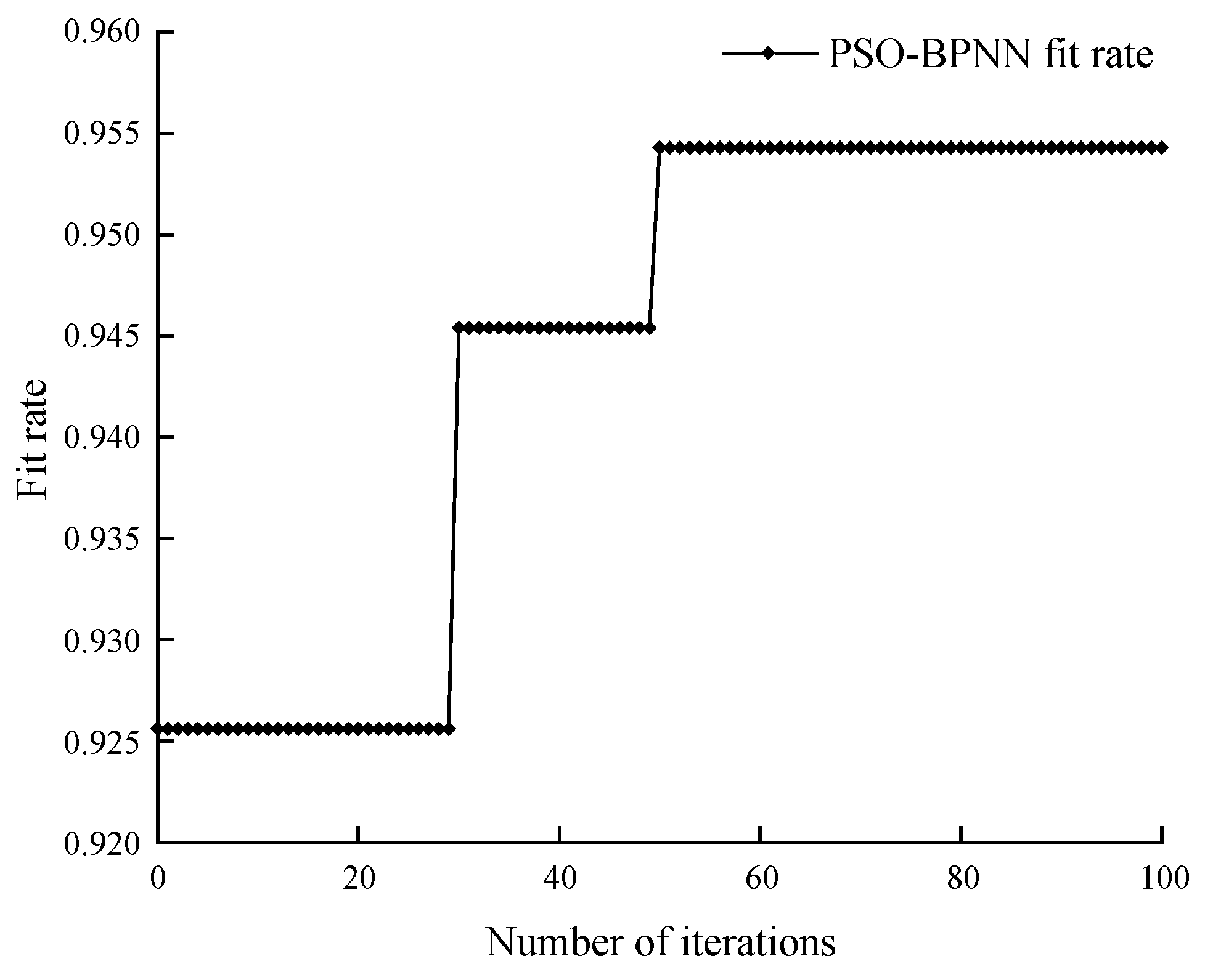
The PSO-BPNN prediction model was constructed by utilising the MATLAB software, setting the number of neurons in the hidden layer to 20, the maximum number of iterations to 1000, the learning rate to 0.01, the error threshold to 0.0000001, the learning factors to 2, the population to 5, and the number of population updates to 30. The specific parameter settings are shown in

Table 5. Parameter setting of the PSO-BPNN model.

Parameter	Specific Values
Population size	5
Maximum number of iterations	1000
Learning rate	0.01
Error threshold	0.0000001
Learning factors	2
Number of population updates	30

. The iteration process of the PSO-BP neural network is shown in Figure 2, and when the number of iterations reaches 100, the fitting rate reaches 0.9543. The comparison between the predicted and true values obtained from the PSO-BPNN model is shown in

Table 6. Comparison between real values and predicted values of the PSO-BPNN model.

No.	True Values /cm3·cm−2·s−1	Prediction Values /cm3·cm−2·s−1	Absolute Error	Relative Error/%
1	1.88	1.9263	0.0463	2.46
2	3.52	3.5737	0.0537	1.53
3	4.24	4.2859	0.0459	1.08
4	6.01	6.0041	0.0059	0.10
5	3.76	4.1511	0.3911	10.40

. As shown in Table 6, the relative error between the predicted value and the true value is between 0.10% and 10.40%, with a difference of 10.30% and an average relative error of 3.11%; its absolute error is between 0.0059 and 0.3911, with a difference of 0.3852 and an average absolute error of 0.1086. The absolute error, as shown in Table 6, is the absolute value of the difference between the true value and the predicted value.

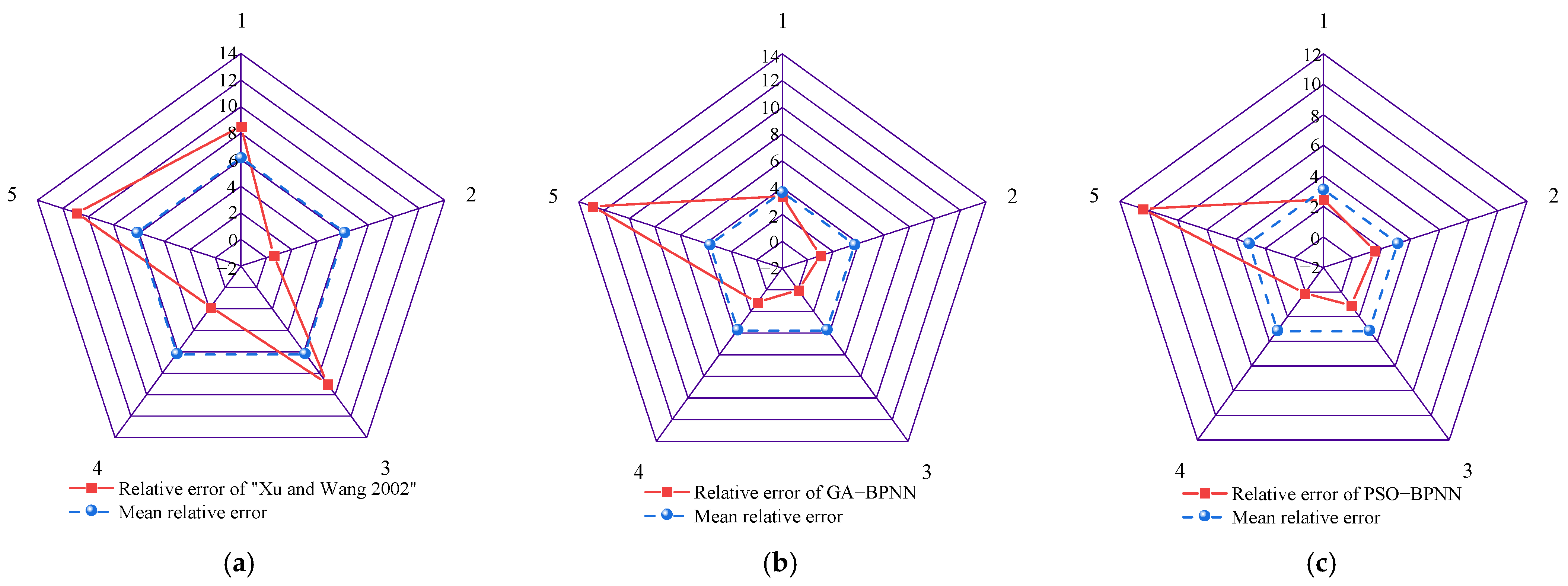
The relative error and average relative error of the prediction results of each model are shown in Figure 3. As can be seen from Figure 3, after GA and PSO optimization, the average relative error of the prediction results is significantly better than that of the BP neural network in the reference [9], and the results of the PSO optimization are better than the GA optimization, which indicates that the optimized BP neural network overcomes the original shortcomings.

3. The GA-SVM Prediction Model

3.1. Support Vector Machine

Support vector machine (SVM) is a machine learning method based on the VC-dimensional theory of statistical learning theory and the principle of structural risk minimization proposed by Vapnik in the 1990s [23]. The learning method takes the classification hyperplane as the decision surface in the mapping process to achieve the optimal linear regression function, which makes it useful for nonlinear regression problems [23].

Suppose the training set samples are {(x₁, y₁), (x₂, y₂), …, (x_m, y_m)}, where x_i ∈ R^m is the input vector, y_i ∈ R^m is the target value, and m is the number of samples. According to the nonlinear mapping, Φ: x ∈ R^m → F, the high-dimensional feature space F is constructed. Based on the principle of minimizing structural risk, the objective function is as follows:

$$\begin{array}{cccc}\min \frac{1}{2}{\Vert \omega \Vert }^2+C{\displaystyle \sum _{i=1}^m({\xi }_i+{\xi }_i^{*})}& \{\begin{array}{c}{y}_i-\omega \varphi \left(x_i\right)-b\le \epsilon +{\xi }_i^{*}\\ -y_i+\omega \varphi \left(x_i\right)+b\le \epsilon +{\xi }_i\\ {\xi }_i^{*}\ge 0,{\xi }_i\ge 0\end{array},& i=1,2,\cdots ,m,& C\ge 0\end{array}$$

(8)

where ξ_i and ξ_i^* are non-negative relaxation functions, C is the penalty factor, ε is the parameter of the loss function, and ‖ω‖ is the model complexity descriptor function.

3.2. Optimization of the SVM by the GA

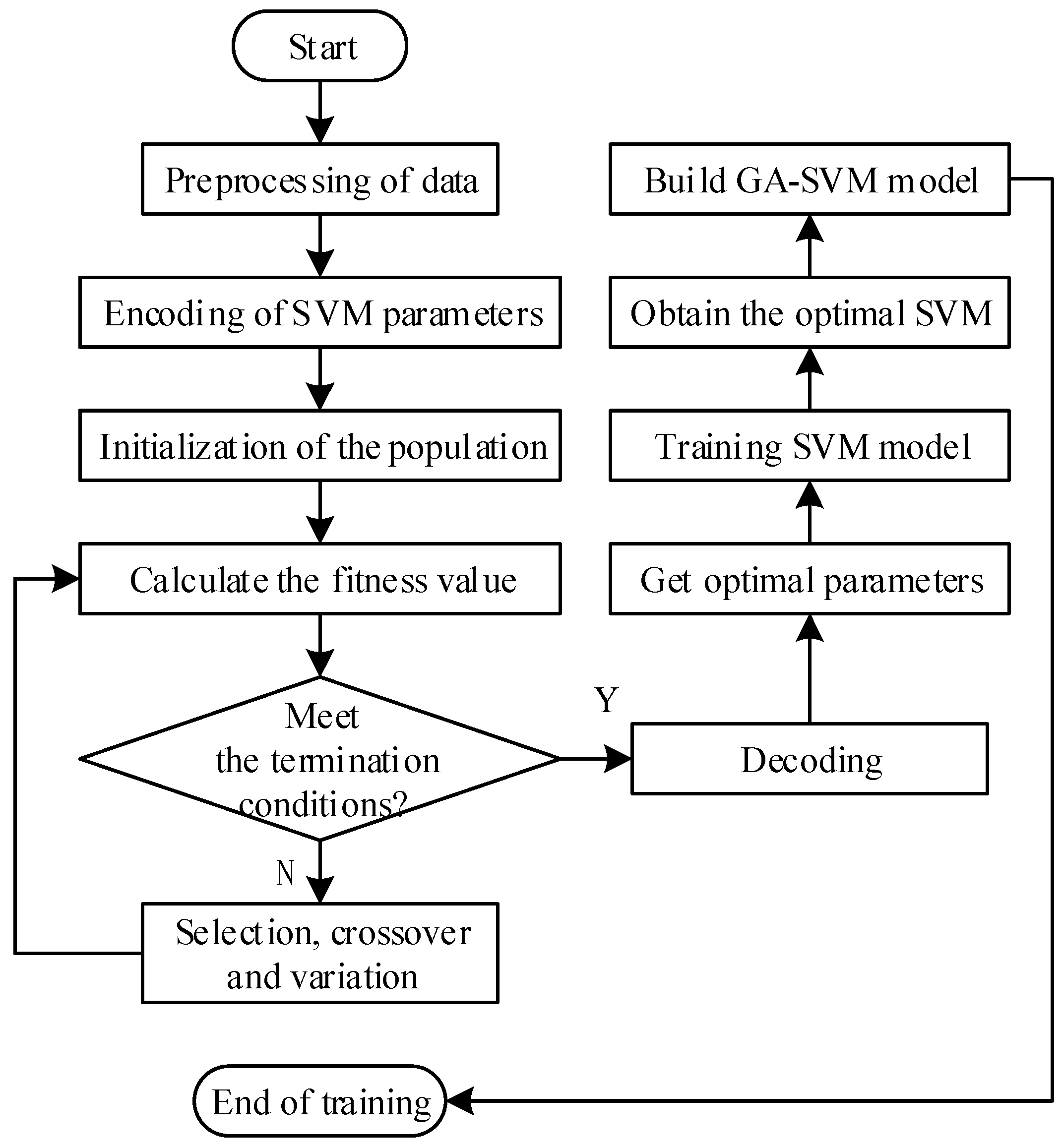
The model parameters of the SVM were optimized by global search ability and implicit parallelism and other advantages of the GA. The prediction model of coal spontaneous combustion limit parameters was constructed based on the GA-SVM. The computational flow of the GA-SVM model is shown in Figure 4, and the main steps are as follows:

(1)

Normalize the sample data and divide the training and test sets;

(2)

Encode the type of kernel function, kernel parameters, and penalty factors of the SVM in the binary coding manner and generate the initialization population,

(3)

Determine the fitness function and calculate the fitness value,

(4)

Determine whether the condition of termination is reached or not. If so, carry out the decoding operation; if not, perform selection, crossover, and mutation to form a new population and go to step (3), until the condition of termination is satisfied,

(5)

Train the SVM model by decoding to obtain the optimal parameters, and then train the GA-SVM model by obtaining the optimal SVM.

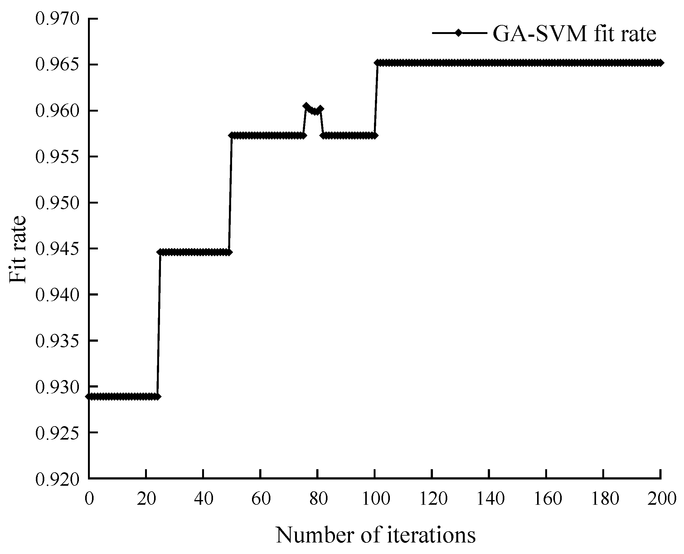
The GA-SVM prediction model was constructed by utilising the MATLAB software. The maximum evolutionary generation of the genetic algorithm was set to 200, the population size was 20, the number of cross-validation v was taken to 5, the range of variation of the penalty coefficient C was [0.1, 100], and the range of variation of the radius of the Gaussian kernel function g was [0.01, 1000]. The specific parameter settings are shown in

Table 7. Parameter setting of the GA-SVM model.

Parameter	Specific Values
Maximum evolutionary generations of the genetic algorithm	200
Population size	20
Number of cross-validations	5
Penalty coefficient	[0.1, 100]
Radius of the Gaussian kernel function	[0.01, 1000]

. The iteration process of the GA-SVM is shown in Figure 5, and when the number of iterations reaches 100, the fitting rate reaches 0.9652. The comparison between the predicted values and true values from the GA-SVM model is shown in

Table 8. Comparison between real values and predicted values of the GA-SVM model.

No.	True Values /cm3·cm−2·s−1	Prediction Values /cm3·cm−2·s−1	Absolute Error	Relative Error /%
1	1.88	1.9354	0.0554	2.94
2	3.52	3.5748	0.0548	1.56
3	4.24	4.4483	0.2083	4.91
4	6.01	6.1503	0.1403	2.33
5	3.76	3.7386	0.0214	0.57

. As can be seen from Table 8, the relative error between the predicted value and the true value is between 0.57% and 4.91%, with a difference of 4.34% and an average relative error of 2.46%; its absolute error is between 0.0214 and 0.2083, with a difference of 0.1869 and an average absolute error of 0.0960. The absolute error, as described above, is the absolute value of the difference between the true value and the predicted value.

4. Forecast Results and Example Analysis

4.1. Analysis of Results

In order to further verify the prediction performance of each model, the GA-BPNN model, the PSO-BPNN model, and the GA-SVM model were used to model, train, and test and analyze the upper limit air leakage intensity in the coal spontaneous combustion limit parameters, respectively, under the condition of the same training and test samples. The prediction results are compared with that of the reference [9]. The methods and models proposed in this article are implemented based on the MATLAB R2021b environment for Windows 10 64-bit system. Four evaluation indexes, mean absolute error (MAE), mean absolute percentage error (MAPE), root mean square error (RMSE), and coefficient of determination (R²), were selected to analyze the performance of the models. By recording the analysis duration of each model,

Table 9. Duration of analysis for each model.

Name of the Method	Duration of the Analysis/s
GA-BPNN	8.35
PSO-BPNN	5.61
GA-SVM	4.11

can be obtained. From Table 9, it can be seen that the GA-SVM model has the shortest analysis duration, indicating that its performance is superior to other models.

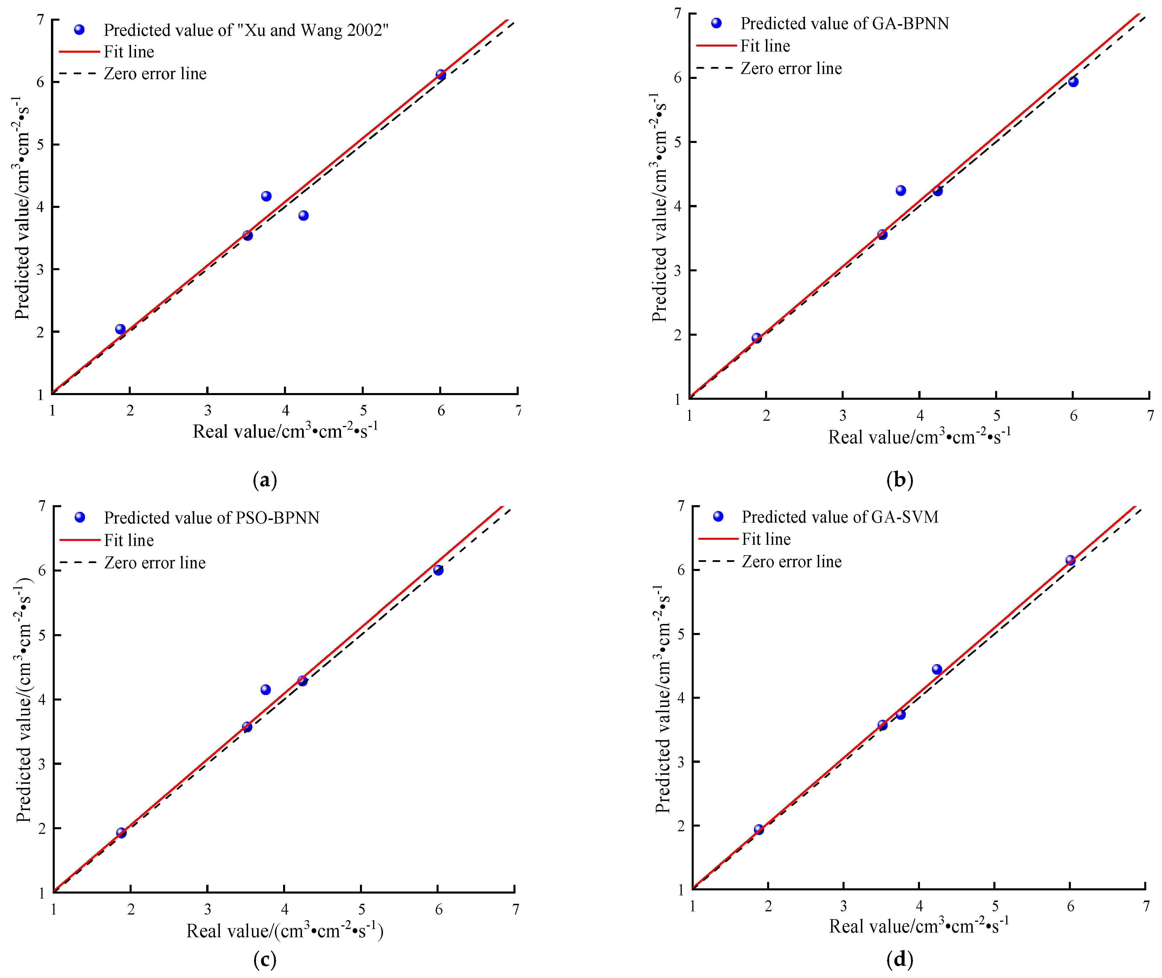
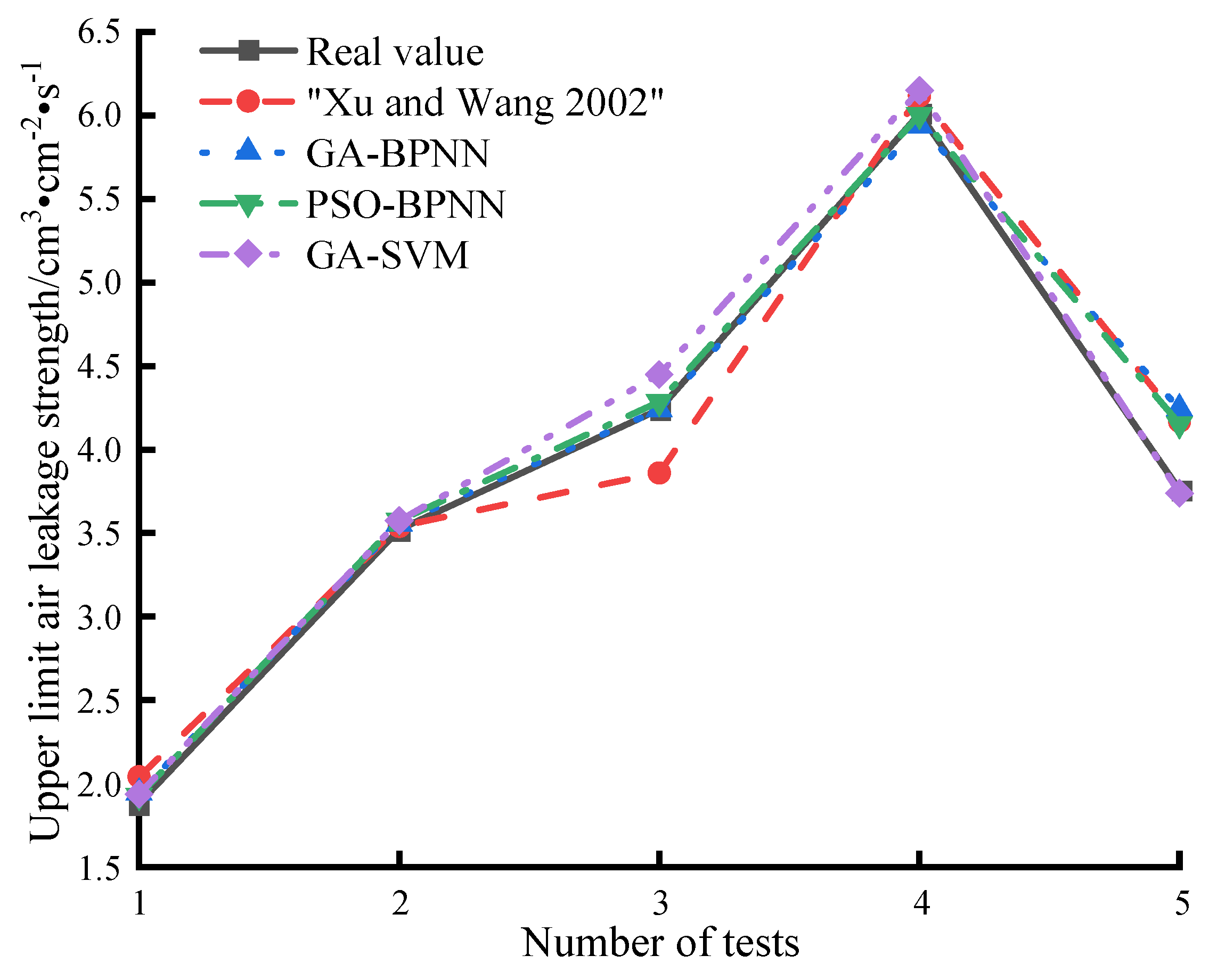
The prediction results of each model are shown in Figure 6, Figure 7 and Figure 8 and

Table 10. Calculation results of prediction performance evaluation indicators.

Models	Performance Index
	MAE	MAPE/%	RMSE	R2
Reference [9]	0.2160	6.16	0.2648	0.9602
GA-BPNN	0.1309	3.69	0.2212	0.9722
PSO-BPNN	0.1086	3.11	0.1789	0.9818
GA-SVM	0.0960	2.46	0.1180	0.9921

, respectively. Figure 6 shows the fitting curves of the prediction results of each model. From Figure 6, it can be seen that the GA-SVM model has the best fitting results between the output and the target value, while the fitting effect of the PSO-BPNN model, the GA-BPNN model, and reference [9] decrease in order, indicating that there is the best result for the training of the PSO-BPNN model. Figure 7 shows the comparison of the prediction results of each model, which indicates that, although there is a deviation between the predicted values and the real data of each model, the overall trend of change is consistent. There is the largest deviation in the results of the reference [9], while there is the smallest deviation in that of the GA-SVM model, and the change rule of prediction values of the GA-SVM model is closer to that of the real data.

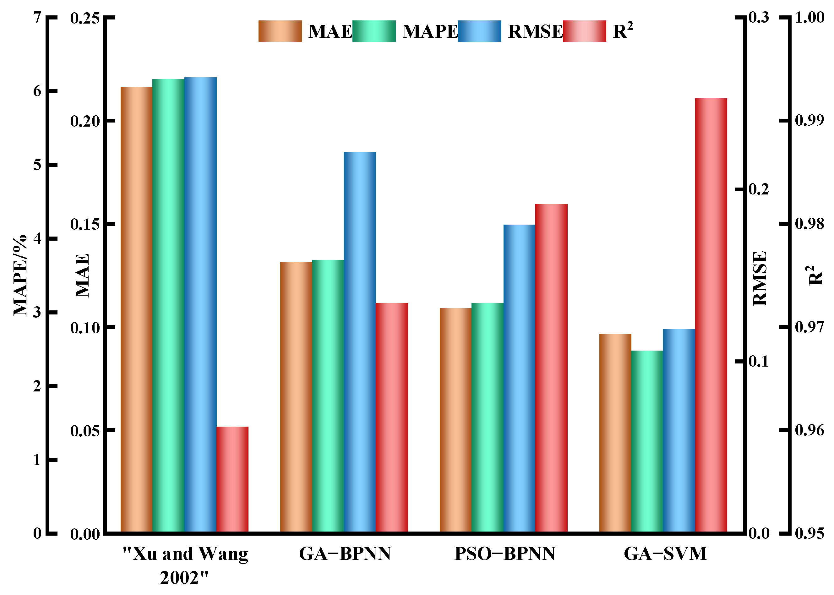
Table 10 shows the calculation results of the prediction performance evaluation indexes of each model, and Figure 8 shows the comparison of the prediction performance evaluation indexes of different models. According to Table 10 and Figure 8, it can be found that the MAPE of the prediction results in the reference [9] is 6.16%, MAE is 0.2160, RMSE is 0.2648, and R² is 0.9602. The MAPE predicted by the GA-BPNN model is 3.69%, the MAE is 0.1309, the RMSE is 0.2212, and R² is 0.9722. The MAPE predicted by the PSO-BPNN model is 3.11%, the MAE is 0.1086, the RMSE is 0.1789, and R² is 0.9818. The MAPE predicted by the GA-SVM model is 2.46%, the MAE is 0.0960, the RMSE is 0.1180, and R² is 0.9921. Compared with the reference [9], the GA-BPNN model and the PSO-BPNN model, the MAPE of the GA-SVM model is reduced by 3.70%, 1.23%, and 0.65%, respectively; the MAE is reduced by 0.12, 0.0349, and 0.0126, respectively; the RMSE is reduced by 0.1468, 0.1032, and 0.0609, respectively; and the R² is increased by 0.0319, 0.0199, and 0.0103, respectively. The prediction results of the GA-SVM model are better than that of other models, which proves that the GA-SVM model is more accurate than the others in the prediction of the parameters of the spontaneous combustion limit of coal.

4.2. Example Applications

In order to further illustrate the universality and stability of the prediction model of the limit parameters of coal spontaneous combustion, the data of the minimum residual coal thickness in a goaf of Z109 fully comprehensive caving work face in a coal mine in Shanxi province were selected for verification. The Z109 working face is located in the No. 22 coal seam of No. 1 mining area with U-type ventilation of the actual air supply to 1200 m³/min and the length of the working face to 86 m. The mining method is comprehensive mechanized top coal caving technology; the maximum mining height of the coal mining machine is 3.5 m with the advancing speed to 5.5 m/d. The spontaneous combustion tendency of the mined coal seam is II, which is spontaneous combustion coal seam with the shortest natural ignition period of 80 d.

The data of the minimum residual coal thickness were put to the BPNN model, the GA-BPNN model, the PSO-BPNN model, and the GA-SVM model for comparative analysis. The prediction results of each model are shown in

Table 11. Prediction results of the different models.

No.	True Values/m	BPNN		GA-BPNN		PSO-BPNN		GA-SVM
		Prediction Values/m	Relative Error/%	Prediction Values/m	Relative Error/%	Prediction Values/m	Relative Error/%	Prediction Values/m	Relative Error/%
1	0.53	0.56	5.66	0.4747	10.44	0.5095	3.86	0.5101	3.76
2	0.77	0.74	3.90	0.7706	0.08	0.7664	0.47	0.7834	1.75
3	0.84	0.90	7.14	0.8546	1.74	0.8353	0.56	0.8534	1.59
4	0.73	0.68	6.85	0.7163	1.88	0.7173	1.74	0.7417	1.60
5	1.11	1.14	2.70	1.0981	1.07	1.1592	4.43	1.0878	2.00

, and the average relative error and R² are shown in Figure 9. The results show that the GA-SVM model is optimal in terms of both average relative error and R², followed by the PSO-BPNN model and the GA-BPNN model, with the BPNN model bringing up the rear. It is proved that the GA-SVM model is optimal in terms of accuracy with good universality and stability.

5. Conclusions

In this paper, the GA-BPNN prediction model, PSO-BPNN prediction model, and GA-SVM prediction model of coal spontaneous combustion limit parameter are constructed, and the main conclusions obtained by comparing and analyzing the prediction results of each prediction model are as follows:

(1)

A coal spontaneous combustion limit parameter prediction model is proposed based on BP neural network. Two optimization algorithms, GA and PSO, are applied to improve the BP neural network, respectively. The results show as follows: after optimization of the GA and the PSO, the BP neural network overcomes the shortcomings, such as slow convergence and local optimum. The prediction results of the BP neural network optimized by the PSO are better than those optimized by the GA;

(2)

Comparing the prediction results of each prediction model with those in the reference [9], the results show the following: the MAE, MAPE, and RMSE of the GA-SVM model are reduced by 0.0126, 0.65%, and 0.0609 than the PSO-BPNN model, respectively; the R² is increased by 0.0103 than the PSO-BPNN model. Compared with the GA-BPNN model, the MAE, MAPE, and RMSE were reduced by 0.0349, 1.23%, and 0.1032, respectively, with R² increasing by 0.0199. Compared to reference [9], the MAE, MAPE, and RMSE were reduced by 0.12, 3.70%, and 0.1468, respectively, with R² increasing by 0.0319. Therefore, the prediction results of the GA-SVM model are superior to all other models, followed by the PSO-BPNN model, with reference [9] bringing up the rear, which indicates that the GA-SVM model can effectively improve the accuracy of the prediction of the parameters of the spontaneous combustion limit of coal;

(3)

To further verify the universality and stability of the GA-SVM model, it is applied to the prediction of the minimum coal thickness in the goaf of a coal mine in Shanxi. Compared with other prediction models, the results show that the prediction effect of the GA-SVM model is optimal over the other models, indicating that the GA-SVM model is more accurate in predicting the parameters of the spontaneous combustion limit of coal.

References

1. Zhang, Y.; Niu, K.; Du, W.; Zhang, J.; Wang, H.; Zhang, J. A method to identify coal spontaneous combustion—Proneregions based on goaf flow field under dynamic porosity. Fuel 2021, 288, 119690. [Google Scholar] [CrossRef]
2. Wang, W.; Qi, Y.; Jia, B.; Yao, Y. Dynamic prediction model of spontaneous combustion risk in goaf based on improved CRITIC-G2-TOPSIS method and its application. PLoS ONE 2021, 16, e0257499. [Google Scholar] [CrossRef] [PubMed]
3. Li, S.; Xu, K.; Xue, G.; Liu, J.; Xu, Z. Prediction of coal spontaneous combustion temperature based on improved grey wolf optimizer algorithm and support vector regression. Fuel 2022, 324 Pt B, 124670. [Google Scholar] [CrossRef]
4. Qi, Y.; Wang, W.; Qi, Q.; Ning, Z.; Yao, Y. Distribution of spontaneous combustion three zones and optimization of nitrogen injection location in the goaf of a fully mechanized top coal caving face. PLoS ONE 2021, 16, e0256911. [Google Scholar] [CrossRef] [PubMed]
5. Wang, Y.-C.; Zhong, K.-Q.; Xiao, Y.; Lai, X.-P.; Li, Q.-W. Determining the Spontaneous Combustion Period and Limit Parameters of Coal: A Large-Scale Furnace Experiment. Combust. Sci. Technol. 2023, 195, 494–507. [Google Scholar] [CrossRef]
6. Wang, W.; Qi, Y.; Liu, J. Study on multi field coupling numerical simulation of nitrogen injection in goaf and fire-fighting technology. Sci. Rep. 2022, 12, 17399. [Google Scholar] [CrossRef]
7. Qiao, M.; Ren, T.; Roberts, J.; Yang, X.; Li, Z.; Wu, J. New insight into proactive goaf inertisation for spontaneous combustion management and control. Process Saf. Environ. Prot. 2022, 161, 739–757. [Google Scholar] [CrossRef]
8. Yan, H.; Nie, B.; Kong, F.; Liu, Y.; Liu, P.; Wang, Y.; Chen, Z.; Yin, F.; Gong, J.; Lin, S.; et al. Experimental investigation of coal particle size on the kinetic properties of coal oxidation and spontaneous combustion limit parameters. Energy 2023, 270, 126890. [Google Scholar] [CrossRef]
9. Xu, J.; Wang, H. The neural network prediction method for the limit parameters of coal self-ignition. J. China Coal Soc. 2002, 27, 366–370. [Google Scholar] [CrossRef]
10. Deng, J.; Ren, S.; Ren, L.; Wang, C.; Li, Q. Hazard indicators and limit parameters of coal spontaneous combustion in Eastern Sichan. J. Xi’an Univ. Sci. Technol. 2021, 42, 196–202. [Google Scholar] [CrossRef]
11. Meng, Q.; Wang, H.; Wang, Y.; Zhou, Y. Predicting limit parameters of coal self-ignition based on support vector machine. J. China Coal Soc. 2009, 34, 1489–1493. [Google Scholar] [CrossRef]
12. Wang, C.; Zhao, X.; Bai, Z.; Deng, J.; Shu, C.-M.; Zhang, M. Comprehensive index evaluation of the spontaneous combustion capability of different ranks of coal. Fuel 2021, 291, 120087. [Google Scholar] [CrossRef]
13. Zhang, Y.; Zhang, Y.; Li, Y.; Li, Q.; Zhang, J.; Yang, C. Study on the characteristics of coal spontaneous combustion during the development and decaying processes. Process Saf. Environ. Prot. 2020, 138, 9–17. [Google Scholar] [CrossRef]
14. Zhang, F. Limit parameter changes and hazardous area determination of residual coal spontaneous combustion in compound goaf. Min. Saf. Environ. Prot. 2020, 41, 66–72. [Google Scholar] [CrossRef]
15. Wang, Y.; Wang, J.; Zou, Z.; Liu, Q. Study on spontaneous combustion characteristics and limit parameters of coal in high geothermal mine. Coal Technol. 2020, 39, 90–93. [Google Scholar] [CrossRef]
16. Zhang, X.; Zhu, H.; An, Q.; Li, X.; Cheng, W.; Dou, K. Analysis on limit parameters of coal spontaneous combustion in goaf of Kaida coal mine. J. Saf. Sci. Technol. 2021, 17, 86–92. [Google Scholar] [CrossRef]
17. Wang, J.; Su, H.; Li, J.; Zou, L.; Ren, L. Effect of sulfur content on characteristics and limiting parameters of coal spontaneous combustion. Saf. Coal Mines 2020, 51, 43–48. [Google Scholar] [CrossRef]
18. Zhou, X.; Niu, T.; Bai, G.; Li, A.; Wang, C. Study on influence of air supply on limit parameters of spontaneous combustion of lignite. J. Saf. Sci. Technol. 2018, 14, 82–86. [Google Scholar] [CrossRef]
19. LeCun, Y.; Bengio, Y.; Hinton, G. Deep learning. Nature 2015, 521, 436–444. [Google Scholar] [CrossRef]
20. Will, S. Fintech model: The random neural network with genetic algorithm. Procedia Comput. Sci. 2018, 126, 537–546. [Google Scholar] [CrossRef]
21. Mahya, M.; Alireza, A.; Masoud, R. Transmission and generation expansion planning of energy hub by an improved genetic algorithm. Energy Sources Part A Recovery Util. Environ. Eff. 2019, 41, 3112–3126. [Google Scholar] [CrossRef]
22. Zhang, Z.; Jia, L.M.; Qin, Y. Modified constriction particle swarm optimization algorithm. J. Syst. Eng. Electron. 2015, 26, 1107–1113. [Google Scholar] [CrossRef]
23. Cao, Y.; Yin, K.; Zhou, C.; Ahmed, B. Establishment of landslide groundwater level prediction model based on GA-SVM and influencing factor analysis. Sensors 2020, 20, 845. [Google Scholar] [CrossRef] [PubMed]
Figure 1. Iterative process of the GA-BP neural network.
Fire 06 00381 g001
Figure 2. Iterative process of the PSO-BP neural network.
Fire 06 00381 g002
Figure 3. Relative error of the predicted results of each model. (a) Relative error of the BPNN model in reference [9]. (b) Relative error of the GA−BPNN model. (c) Relative error of the PSO−BPNN model.
Fire 06 00381 g003
Figure 4. Calculation process of the GA-SVM model.
Fire 06 00381 g004
Figure 5. Iterative process of GA- SVM.
Fire 06 00381 g005
Figure 6. Fitting curves of the predicted results of each model. (a) Reference [9]. (b) GA-BPNN. (c) PSO-BPNN. (d) GA-SVM.
Fire 06 00381 g006
Figure 7. Comparison curves of prediction results of each model. “Xu and Wang 2022” is the upper limit air leakage strength of the BPNN model in reference [9].
Fire 06 00381 g007
Figure 8. Comparison of prediction performance evaluation indicators of different models. “Xu and Wang 2022” is the prediction results of the BPNN model in reference [9].
Fire 06 00381 g008
Figure 9. Comparison of the various model indicators.
Fire 06 00381 g009