Article

Summer and Fall Extreme Fire Weather Projected to Occur More Often and Affect a Growing Portion of California throughout the 21st Century

1
Department of Geography, San Diego State University, San Diego, CA 92182, USA
2
Department of Geography, University of California Santa Barbara, Santa Barbara, CA 93106, USA
*
Author to whom correspondence should be addressed.
Fire 2022, 5(6), 177; https://doi.org/10.3390/fire5060177
Submission received: 15 September 2022 / Revised: 10 October 2022 / Accepted: 25 October 2022 / Published: 27 October 2022
(This article belongs to the Special Issue Fire in California)

Abstract

:
Annual burned area has increased in California over the past three decades as a result of rising temperatures and a greater atmospheric demand for moisture, a trend that is projected to continue throughout the 21st century as a result of climate change. Here, we implement a bias-correction and statistical downscaling technique to obtain high resolution, daily meteorological conditions for input into two fire weather indices: vapor pressure deficit (VPD) and the Canadian Fire Weather Index System (FWI). We focus our analysis on 10 ecoregions that together account for the diverse range of climates, ecosystems, topographies, and vegetation types found across the state of California. Our results provide evidence that fire weather conditions will become more extreme and extend into the spring and fall seasons in most areas of California by 2100, extending the amount of time vegetation is exposed to increased atmospheric demand for moisture, and heightening the overall risk for the ignition and spread of large wildfire. The ecoregion-level spatial scale adopted for this study increases the spatial specificity of fire weather information, as well as the resolution with which fire and land managers can implement strategies and counter-measures when addressing issues related to climate change.

1. Introduction

Numerous research studies indicate that wildfire activity in the western United States has increased over the past few decades due primarily to increases in temperature, decreases in precipitation, and increases in atmospheric aridity [1,2,3,4,5]. Furthermore, by the end of the 21st century, anthropogenic global warming will contribute to increased risk of extreme fire weather through the effect of rising temperatures [6]. However, the impacts of climate on fire regime vary dramatically by ecosystem, predominant vegetation types, topography, and human activity. These complex relationships between climate and wildfire are apparent in California, where climate, vegetation, and topography vary significantly from east to west and north to south.
For example, large parts of southern California experience near continuous high fire danger in the summer and fall, as high temperatures, seasonal drought, and the onset of the Santa Ana wind season combine to increase the risk of severe wildfire. In these areas, wildfire is rarely limited by weather conditions governing fire spread, but by availability of fuel to burn. On the other hand, in forested ecosystems, where deep rooted vegetation is less susceptible to short-term variations in moisture, the limiting factor may be fire spread potential or dried fuel available to burn [7,8]. Therefore, the effects of climate change on wildfire in California, specifically projected increases in temperature and aridity, will not impact all ecosystems equally, but will be strongly dependent on vegetation distribution and will be more likely to place flammability-limited ecosystems (i.e., forested) at a greater risk for catastrophic wildfire [9,10]. Furthermore, understanding the broad range of outcomes regarding the impacts of climate change on extreme fire weather risk is critical because climate change may lead to the loss of existing climate regimes and the emergence of novel ecosystem states, impacting the distribution of biomass (i.e., continuity and flammability), fire spread potential, and ignition [11,12].
One of the most valuable tools for assessing historical and projected climate variability, especially the meteorological variables that govern wildfire on a regional scale, are global climate models, or GCMs [13]. The Climate Model Intercomparison Project (CMIP) provides a standardized platform for the collection and analysis of GCM model output with the intent of studying natural and anthropogenic climate variability. The most recent release of GCM output for the CMIP Phase 6 provides a new suite of climate model data for use in a wide range of disciplines. While GCMs are often used for the evaluation of long-term variations in climate, there are significant limitations to their use for the study of wildfire impact assessment and fire weather potential. The main limitation is that climate model output is typically of coarse resolution and is subject to significant bias [13]. The mismatch between the spatial scale at which key variability in fire weather variables fluctuate (<10 km), and that of GCM output (>100 km), creates a need to account for these spatial differences.
One method of adjusting the resolution of available GCM output to that which is needed for the evaluation of fire weather variables is statistical downscaling. These methods allow for the reduction in systematic biases inherent to numerical weather prediction systems, as well as an enhancement of grid cell resolution in order to account for the effects of topography and other land surface features [14]. One method of statistical downscaling for use in wildfire risk assessment is bias correction and spatial downscaling (BCSD) [13]. BCSD is a two-step process that involves the bias correction of coarse GCM data using local observations that have been aggregated to the model’s resolution [13]. Bias correction techniques include scaling, delta methods, and empirical quantile mapping. In addition, spatial downscaling utilizes techniques such as linear or multiple regression to apply statistical relationships (e.g., slope, y-intercept) derived from high resolution observational data to coarse resolution GCM data in order to improve the resolution [15]. The major assumption made with statistical downscaling methods is that of climate stationarity. It is assumed that the relationships between the coarse and fine scale historical datasets, calculated by the statistical model, will stay the same in the future (with climate change), and that when these models are applied to projected datasets the outcomes will be valid [13,14,15].
In order to track changes in, and probability of, extreme fire weather over time, fire weather indices are often calculated using weather station, reanalysis, or global climate model data. Two commonly used fire weather indices are vapor pressure deficit (VPD) and the Canadian Fire Weather Index System (CFWIS) [16,17]. The CFWIS relies on regular inputs of noon-day temperature, 24 h precipitation accumulation, 10 m wind speed, and relative humidity, and is comprised of six components: three fuel moisture codes and three fire behavior metrics, with the primary purpose of assessing the effect of weather on fuels and potential fires. In general, higher values indicate a more severe risk for ignition or spread of large wildfire [17,18].
On the other hand, VPD, defined as the difference between saturation vapor pressure and actual vapor pressure, is a commonly used metric for the quantification of atmospheric aridity in relation to wildfire risk assessment, and is highly correlated with annual area burned [1,2,19]. VPD accounts for the non-linear (exponential) relationship between saturation vapor pressure and temperature, thus better representing moisture stress and flammability [19]. In fact, maximum VPD in the entire United States is found each year in the desert southwest region, not only affecting agricultural production via crop health but increasing the risk of wildfire ignition and spread [19]. Furthermore, two-thirds of historical (2001–2018) increases in extreme VPD in the western United States is attributable to anthropogenic warming [20].
The objective of this research is to utilize bias correction and statistical downscaling to enhance the spatial representations of CMIP6 simulations for the purposes of assessing the potential impacts of climate change on the occurrence of extreme fire weather. Bias corrected and statistically downscaled daily CMIP6 data (~4 km spatial resolution), covering an historical (1981–2010), mid-century (2041–2070), and late-century (2071–2100) period, will be used as input for two fire weather indices, including the Canadian Fire Weather Index (CFWIS; now referred to as FWI) and vapor pressure deficit (VPD). In order to determine the effects of climate change on the occurrence of extreme fire weather in California ecoregions, we investigate the frequency at which daily index values exceed the average daily historical 95th percentile. We also calculate the extent of each ecoregion that is likely to experience values greater than the 30 year average spatial 95th percentile value for each time period. In addition, time series analysis includes fire weather anomalies relative to an historical period, as well as 30 year Julian-day averages. The diversity of factors that influence fire regime in California, as well as the immense range of biophysical characteristics, require an ecoregion scale analysis. The effects of climate change on extreme fire weather will not be homogeneous, however, our fine scale analysis will allow policy makers and land managers to anticipate changes in climate and determine the areas that are most likely to experience the consequences of increased fire potential.

2. Materials and Methods

2.1. Study Area

The primary study area is California (Figure 1). We chose to analyze the effects of climate change on extreme fire weather within ten ecoregions of California [21,22]. These regions include the Southern California Mountains (SCM), Southern California Coast (SCC), Central California Foothills (CCF), Central Valley (CV), North American Desert (NAD), Sierra Nevada (SN), Klamath (K), Cascades (C), East Cascades (EC), and Marine West Coast Mountains (MWCM).
Each of these regions is characterized by different dominant ecosystem types that give rise to California’s diverse fire regimes, including vegetation, climate, soil types, land use, and hydrology [22]. An ecoregion specific analysis will allow for a nuanced understanding of how climate change may impact extreme fire weather relative to historical conditions within homogeneous regions of particular climate and vegetation types.

2.2. Statistical Downscaling Method

Daily near surface maximum air temperature, 24 h precipitation accumulation, 10 m wind speed, and 2 m relative humidity were acquired for three CMIP6 models (including MIROC6, EC-Earth3, and MRI-ESM2-0), for an historical (1981–2010), mid-century (2041–2070), and late-century (2071–2100) period, from the data repository at the Earth System Grid Federation (https://esgf-node.llnl.gov/search/cmip6/, accessed on 1 January 2021). We derived daily relative humidity from specific humidity, sea level pressure, geopotential height, and near surface air temperature. Future climate projections for a mid- and late-century period were obtained for the Representative Concentration Pathway (RCP8.5), “high emissions” scenario. All bias correction and downscaling methods were completed using a 4 km gridded meteorological climate dataset called gridMET [23]. We used the entirety of the gridMET historical period (i.e., 1979–2014) to train the bias correction algorithm, and in order to avoid training and testing our BCSD output with the same data (i.e., gridMET), we validated the results of the BCSD methodology with two independent observational datasets (see Section 2.3).
A bias correction technique known as empirical quantile mapping was applied separately to the four climate variables for each of the three CMIP6 model outputs. This algorithm adjusted the simulation’s (i.e., CMIP6) empirical distribution based on observed patterns (i.e., gridMET) and was used to correct both historic and future climate projections generated by the CMIP6 models [14]. Bias correction methods are often applied to GCM output in order to address inherent biases that arise when modeling earth system processes. The bias corrected GCM data was interpolated to the high-resolution observational grid (i.e., gridMET) using a thin plate spline function and the relationship between the two grids were then estimated to generate regression functions for each grid cell [24]. The linear regression models were then applied to the bias corrected and interpolated GCM data to complete the downscaling.
To elaborate, this spatial downscaling methodology uses regression functions to estimate the linear relationships (in this case the slope and intercept) between the original, high-resolution gridMET data and a “smoothed” estimate, before applying those statistical parameters to the bias-corrected CMIP6 data in a simple linear model to obtain the final downscaled, high-resolution output [25]. For this research, the study area domain was comprised of approximately 70–100 grid cells in the CMIP6 simulations, whereas the gridMET observational data has ~81,000 locations over the same area. In the first step, a thin-plate spline interpolation was used to predict CMIP6 values at the gridMET scale, with no addition of topographic or climatological information. This resulted in “smoothed” CMIP6 data that is identical to the original data but sampled at a much greater frequency. In the next step, a linear regression function was derived from the raw and smoothed gridMET datasets at each grid cell location, for each month of the year (~81,000 grid cells × 12). These month-specific linear regression models were applied to the “smoothed” CMIP6 data to obtain the final downscaled product for each variable.
A square-root transformation was applied to the precipitation data before downscaling to account for its skewed distribution [26,27]. The final bias-corrected and downscaled product of each variable was averaged to obtain an ensemble mean and used in the calculation of the two fire weather indices. Daily maximum temperature, 24 h rainfall, 10 m wind speed, and daily minimum relative humidity were used to calculate FWI, while daily maximum temperature and daily minimum relative humidity are used to calculate VPD. Due to the fact that maximum temperature and minimum relative humidity are used for the calculation of VPD, we make it clear that VPD may be considered “maximum VPD”.

2.3. Climate Model Simulations of Extreme Fire Weather in California Ecoregions

The BCSD CMIP6 GCM data were used for three primary analyses of extreme fire weather in California, as well as an additional analysis of Julian-day climatology. We used maximum daily surface temperature, minimum relative humidity, and 2 pm wind speed, as daily noon-time data requirements were not available for all models. Prior to the analysis, 1979–2014 BCDS product was validated against two observational analysis datasets, the North American Regional Reanalysis (NARR, psl.noaa.gov/data, accessed on 1 March 2022) and TerraClimate [28,29].
Analysis of extreme fire weather consisted of four main components. First, we calculated the June, July, August (JJA) and the September, October, November (SON) seasonal-mean FWI and VPD averages for each ecoregion, as well as for the entire state of California, for an historical (1981–2010), mid-century (2041–2070), and late-century (2071–2100) time period. The historical mean, calculated individually for each ecoregion and for each season, was used as a baseline with which the mid-century and late-century anomalies were calculated. In addition, the relative change (relative to the historical time period) of FWI and VPD in the mid- and late-century periods was calculated. We consider a unique baseline for each ecoregion, in addition to a California state-wide assessment, for each season, in order to properly account for the entire range of climate conditions found across California, and to assess projected changes in each zone relative to their particular local historical climate.
Second, the seasonal, ecoregion specific, daily FWI and VPD averages were used to calculate a 95th percentile value ( F W I 95 ; V P D 95 ), which was then used as a threshold for the mapping of the frequency with which fire weather indices exceed that 95th percentile value during the historical, mid- and late-century periods. The maximum occurrence of a given index value above the 95th percentile is 91, or, in other words, all the days in that season in a given year. In order to evaluate the spatial distribution of extreme fire weather throughout the 21st century, the difference in the total number of days per year that exceed the 95th percentile was taken between the mid- and late-century and the historical period. In addition, the ecoregion average number of days per year that exceed the 95th percentile was calculated.
Third, 30 year JJA and SON seasonal average FWI and VPD were calculated for each ecoregion. Considering all grid points within each ecoregion for that 30 year average, the 95th percentiles are calculated and subsequently used as thresholds to determine the extent within each region that will experience FWI and VPD exceeding those values. Frequency distributions of 30 year spatial average FWI and VPD values were plotted for each ecoregion.
Finally, Julian-day averages spanning the entire 30 year periods were calculated for FWI and VPD. Daily climatologies intend to show changing peaks in average maximum values, as well as the lengthening or shortening of each ecoregion’s fire season.

3. Results

3.1. Validation of Historical Simulations

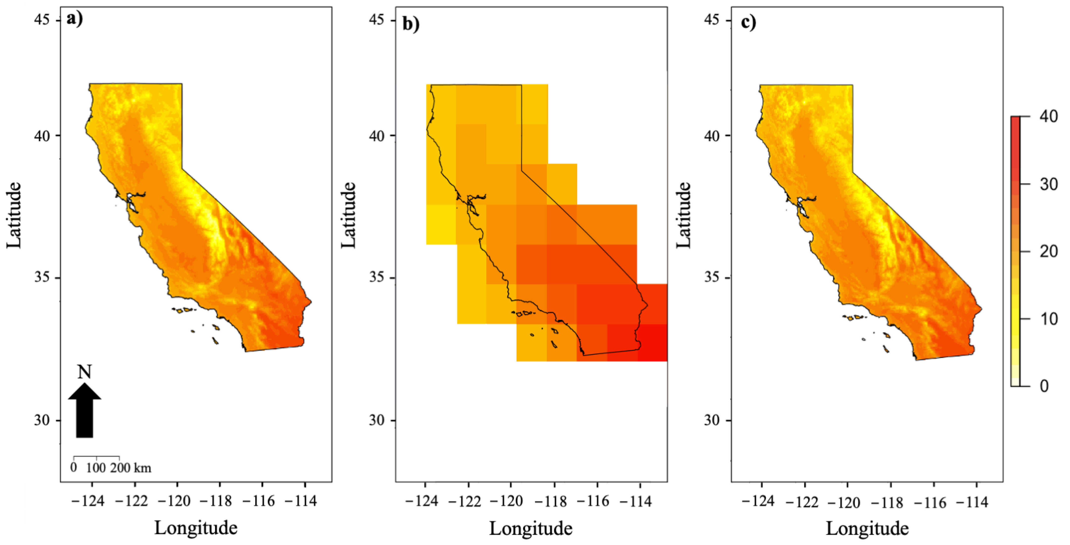
Before investigating the impacts of climate change on extreme fire weather, we evaluate the CMIP6 Raw and BCSD ensembles against an observational ensemble that includes NARR and TerraClimate. However, TerraClimate has not released a minimum relative humidity dataset, so in this case, CMIP6 was validated exclusively with NARR. Spatial statistics, including correlation, bias, and root-mean square error (e.g., sCor, sBias, sRMSE) were calculated after resampling all observations and Raw CMIP6 data to the high resolution BCSD (~4 km). In this way, the improved skill of the bias correction and downscaling was demonstrated against a basic resampling. Temporal statistics (tCor, tBias, tRMSE) were calculated using monthly averages spanning the entire historical period (1979–2014). The difference in resolution between the TerraClimate observations (~4 km), raw MIROC6 (1.4° × 1.4°), and BCSD ensemble (~4 km) are shown below for annual average maximum temperature in 1979 (Figure 2).
Spatial correlations between CMIP6 BCSD and the observations were high for all variables, especially for maximum temperature, precipitation accumulation, and minimum relative humidity, with 0.97, 0.88, and 0.87, respectively—all of which were higher relative to the CMIP6 Raw (Table 1). Furthermore, sRMSE and sBias were higher for the CMIP6 BCSD relative to the CMIP6 Raw for all variables except temperature, which showed a higher sBias in the CMIP6 Raw. A substantially higher sCor and sBias in the wind speed resulted between the Raw and the BCSD, with sCor increasing by 0.4 and sBias by 0.38 (Table 2).
tCor stayed the same for maximum temperature, daily precipitation accumulation and minimum relative humidity, but was higher for wind speed in CMIP6 BCSD relative to the CMIP6 Raw. Similar to the spatial statistics, maximum temperature’s tBias was the only metric that was not lower in the CMIP6 BCSD.
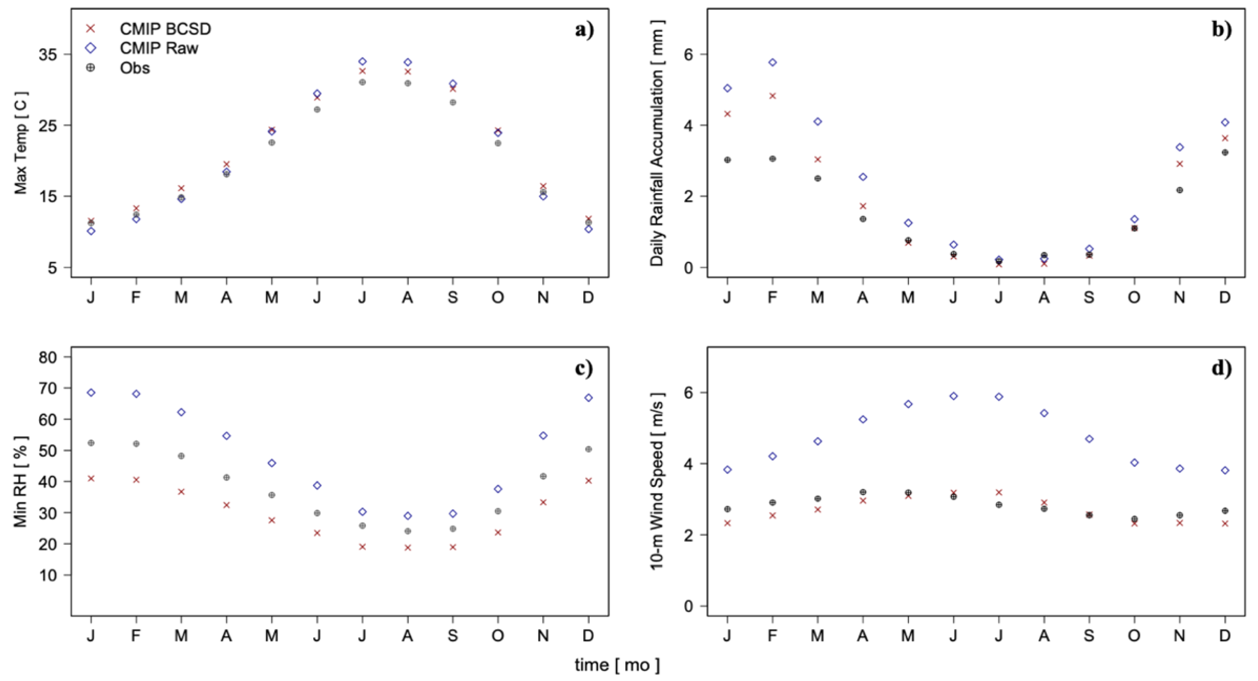
In addition to the statistical metrics, a monthly climatology of each variable was generated for the CMIP6 Raw, CMIP6 BCSD, and the observational ensemble (Figure 3). BCSD successfully shifted the summertime temperatures downwards towards the observations, however, temperatures were slightly overestimated in the winter months (Figure 3a). Both the CMIP6 Raw and BCSD overestimated daily rainfall accumulation in the winter, however, the BCSD more closely approximated the observations throughout the year (Figure 3b).
The NARR minimum relative humidity fell between the CMIP6 Raw and BCSD monthly climatology, however, even though BCSD slightly underestimated winter relative humidity, the difference was smaller in all months than it was for CMIP6 Raw (Figure 3c). CMIP6 BCSD 10 m wind speed was very well simulated in California compared to CMIP6 Raw (Figure 3d).

3.2. Fire Weather Anomalies and Relative Change

FWI time series anomalies indicated increasing trends in both the mid- and late-century periods in all ecoregions, except the MWCM, which displayed a decrease in average FWI relative to the historical period (Figure 4). JJA relative change during the mid-century period ranged from −21.62 in the MWCM to 19.41 in the Central Valley, while late-century change ranged from −20.9 in the MWCM to 21.88 in the Central Valley. Furthermore, mid-century SON relative change ranged from −7.73 in the MWCM to 21.69 in the Cascades, and −8.23 in the MWCM to 25.44 in the Cascades during the late-century period.
Overall, JJA and SON anomalies showed increasing average FWI between 2041–2100 (except MWCM), however, relative change during the SON season was greater than JJA in all ecoregions except the Central Valley during the mid-century period. FWI in the MWCM decreased relative to the historical baseline in both seasons, however, decreases during the SON were of much smaller magnitude, and are basically a continuation of historical conditions. In both the mid- and late-century periods, the central and northern California C, EC, SN, and Central Valley ecoregions experienced greater relative change in FWI compared to the southern California ecoregions SCC and SCM.
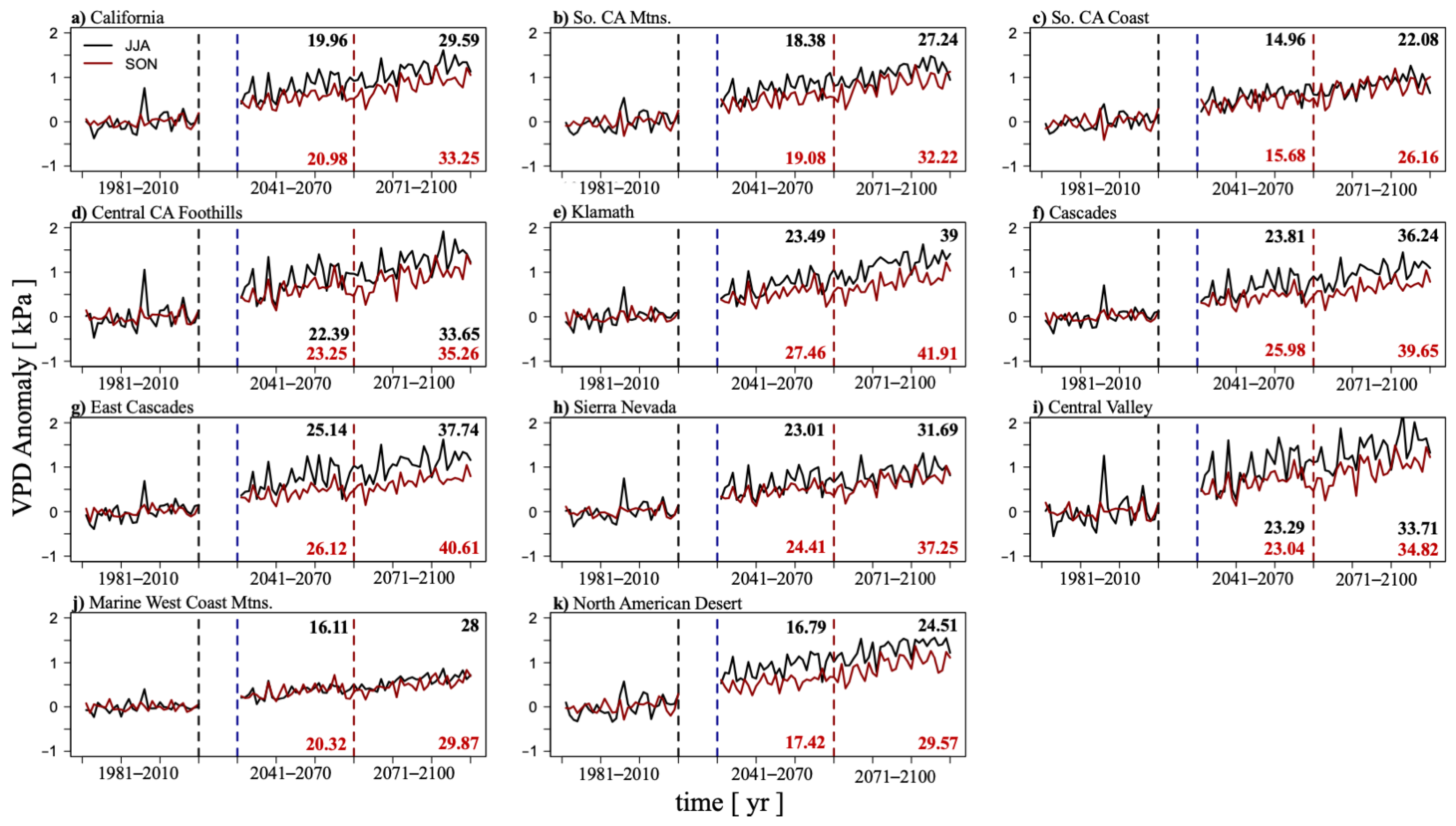
JJA and SON vapor pressure deficit increased relative to an historical baseline in all ecoregions during both the mid- and late-century time periods (Figure 5). Relative change of VPD during the fall was greater than in the summer in all ecoregions. JJA VPD during the mid-century period ranged from 14.96 in the SCC to 25.14 in the EC, and 22.08 in the SCC to 39 in the K during the late-century. On the other hand, mid-century SON vapor pressure deficit ranged from 15.68 in the SCC to 27.46 in the K, and from 26.16 in the SCC to 41.91 in the K ecoregion, during the late-century period.
Similar to FWI, JJA and SON relative change in VPD in the mid- and late-century periods increased more in the central and northern California ecoregions of the K, C, EC, SN, and Central Valley compared to the southern California ecoregions SCC and SCM (Figure 5). While FWI decreased in the MWCM ecoregion relative to its historical baseline (Figure 4j), VPD increased in both the mid- and late-century periods (Figure 5j). Differences between JJA and SON seasonal changes in VPD were greater than for FWI, however lower average historical values during SON led to comparable relative change (to the JJA season) in the mid- and late-century periods. Overall, both JJA and SON vapor pressure deficit is expected to increase linearly throughout 2041–2100, in all ecoregions.

3.3. 95th Percentile Exceedance Maps

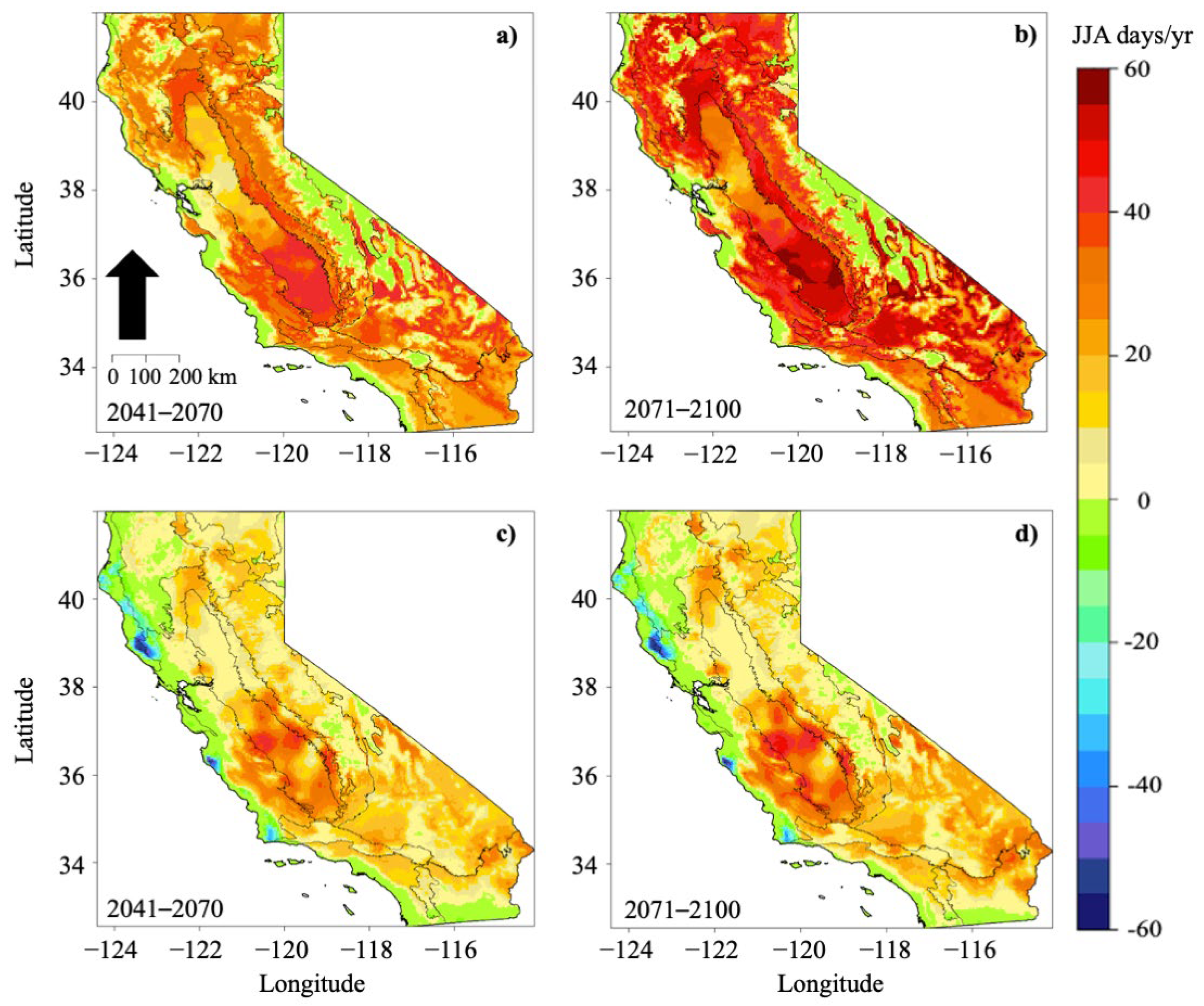
To further investigate the impact of climate change on extreme fire weather, we calculated the number of days that FWI and VPD were greater than or equal to the 95th percentile (calculated using a time series of daily average values for each ecoregion, not per pixel) (Figure 6). On average, JJA V P D 95 days increased substantially in all ecoregions in both the mid- and late-century periods (Table 2). The average number of days per year with VPD greater than the 95th percentile doubled in all ecoregions by 2100. In fact, from 2071–2100, over half the total number of summer days in the CCF, C, EC, CV, and NAD ecoregions had a VPD greater than the historical 95th percentile.
The largest increases in V P D 95 days occurred in the desert southwest region of California, particularly in the late-century period, where some areas are expected to experience historical V P D 95 on nearly two-thirds of all summer days. Other areas expected to experience large increases in V P D 95 days are the SCC ecoregion east of Los Angeles (34° N, 117° W), the southern portion of the Central Valley and the Central California foothills, the western border of the Sierra Nevada, and scattered areas of the northern California Klamath, Cascades, and Eastern Cascades regions (Figure 6a–c).
JJA F W I 95 days increased in both the mid- and late-century in all ecoregions except the MWCM, which experienced an average decrease in F W I 95 days (Table 2). While the increase in average number of days with F W I 95 is smaller than that of V P D 95 , the SCM, C, EC, and CV double the number of F W I 95 days by 2100. In addition, the greatest magnitude of change of F W I 95 days occurred between the historical and the mid-century periods; the total change between the mid- and late-century was much smaller (Table 2). The most substantial increases in F W I 95 days occurred in the desert southwest, the CV, the southern tip of the SN, the CCF, and the C and EC in northern California. However, there was a clear pattern of decreased numbers of F W I 95 and V P D 95 days (particularly FWI) in the mid- and late-century periods along the coast of California where the ocean moderates temperature. Furthermore, there was an apparent influence of topography in northern California (K, C, SN ecoregions), where high elevation areas showed little or even negative change, while, for example, the lower elevation, western slopes of the Sierra Nevada showed pronounced positive change. The dramatic increase in V P D 95 and F W I 95 days in the NAD ecoregion is an important climatic signal for human health and well being, as well as for agriculture, but these increases are not likely to translate into increases in annual area burned because of a near total lack of continuous and flammable vegetation.
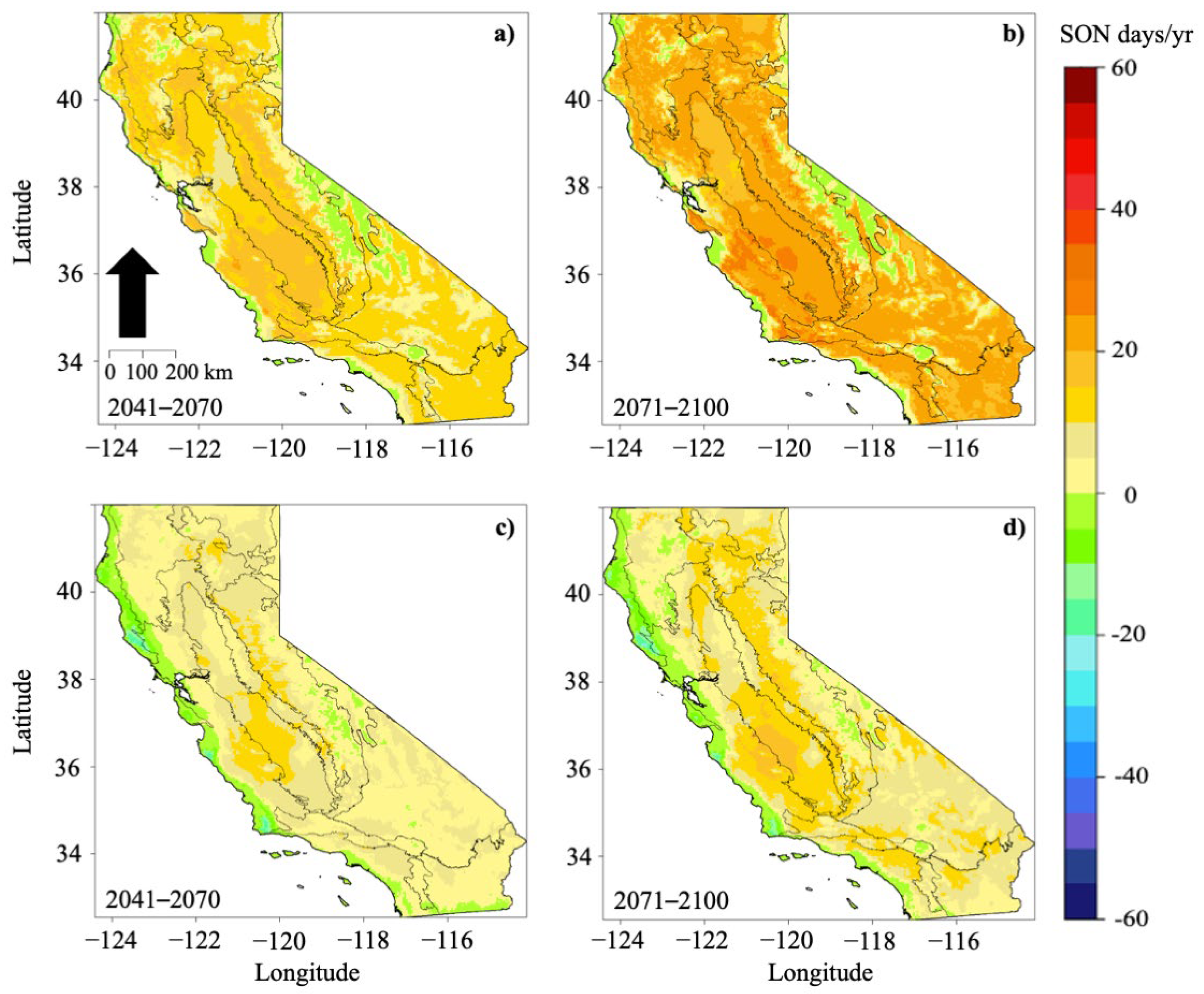
Historical 95th percentile thresholds were also calculated for each ecoregion for the SON season. The average number of V P D 95 days increased in all ecoregions (Table 2). In fact, the average number of V P D 95 days tripled by the end of the late-century period in the CCF, K, C, EC, and CV ecoregions, and doubled in the SCC, SN, MWCM, and NAD ecoregions (relative to the historical period). The average number of V P D 95 days in the late-century period was substantially lower than it was in JJA, however, these results still imply that VPD is expected to increase dramatically for the entire duration of the summer and fall in all ecoregions (Table 2). Increases in the number of SON V P D 95 days occurred in many of the same areas as JJA, including the NAD, the western and lower elevation portions of the Sierra Nevada, the southern region of the Central Valley, the southern California coast, and Central Foothills, as well as large portions of northern California’s ecoregions, including Klamath, Cascades, and Eastern Cascades (Figure 7a–c).
SON F W I 95 days increased in all ecoregions except the MWCM, which decreased from an average of 7 days/yr between 1981–2010 to 3 days/yr between 2071–2100 (Table 2). The C, EC, and CV ecoregions doubled in the number of days experiencing FWI values greater than the historical 95th percentile. Overall changes in the occurrence of F W I 95 days were smaller for the SON season compared to JJA, however, many of the same areas that were impacted in the summer show continued increases in extreme fire weather carrying into the fall, relative to the fall historical 95th percentile (Figure 7f). Some of the most affected areas include the region east of Los Angeles (34° N, 117° W), the south western region of the CCF (35–36° N, 120–121° W), western border of the Sierra Nevada, and the northern California Cascades and Eastern Cascades (Figure 7). Similar to the summer season, there was a moderating influence on FWI along the coast of California, as well as a topographic influence in the K and SN ecoregions. In fact, nearly the entire state of California, apart from the coastal and high elevation areas, displayed a positive signal in V P D 95 by the end of the 21st century.

3.4. Fire Weather Frequency Distributions

The 30 year spatial averages of FWI and VPD were calculated for each of the 10 ecoregions during the historical, mid- and late-century periods. The frequency with which each FWI and VPD value occurred was plotted (as an area), along with the ecoregion specific 95th percentile value and the area that exceeded the threshold value in the three time periods (Figure 8).
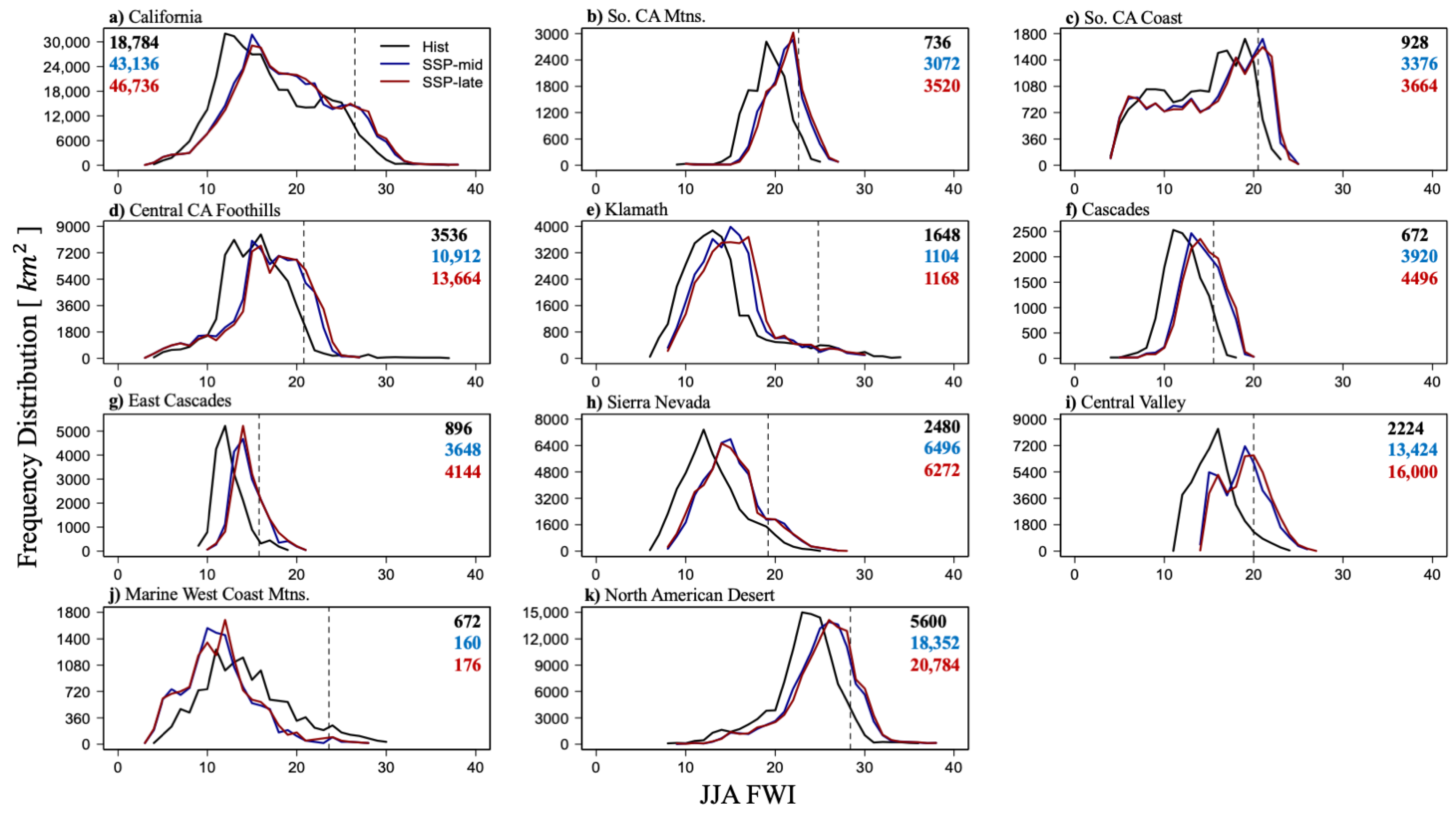
The total land area that was projected to experience FWI greater than the 95th percentile value increased in all ecoregions apart from Klamath and the Marine West Coast Mountains (Figure 8e,j). The largest increases in area occurred in the Central Valley and the Cascades ecoregions (over seven and six times the historical area, respectively). Furthermore, the increase in area experiencing extreme fire weather in the SCM and the EC, followed by the SCC, CCF, and NAD ecoregions, increased by a factor of four and three, respectively. In many cases, including in the SCM, K, C, EC, SN, CV, and NAD ecoregions, the distribution of average FWI values shifted towards the 95th percentile threshold, indicating that mid- and late-century average FWI values could be closer to what is now considered extreme. The JJA F W I 95 percentile values ranged from 15.5 in the Cascades to 28.4 in the North American Desert, while the state-wide California JJA F W I 95 was 26.5.
The increase in the amount of land area likely to experience FWI greater than the historical 95th percentile was even greater for SON than JJA, however, the MWCM ecoregion is projected to have a decline in the total land area with extreme fire weather (Table 3). The ecoregions projected to see the largest changes include the Central Valley, Cascades, and SCM, with ten, eight, and seven times the area under 95th percentile FWI by late-century, relative to the historical period. In addition, the NAD, EC, and SCC ecoregions increased by a factor of six, and the SN by a factor of five. Whereas the area within the Klamath ecoregion with FWI greater than the 95th percentile decreased in the summer, F W I 95 area is projected to double in SON by the end of the late-century. Additionally, the SON F W I 95 percentile values ranged from 8.71 in the Cascades to 16.6 in the North American Desert, while the state-wide California SON F W I 95 was 15.4.
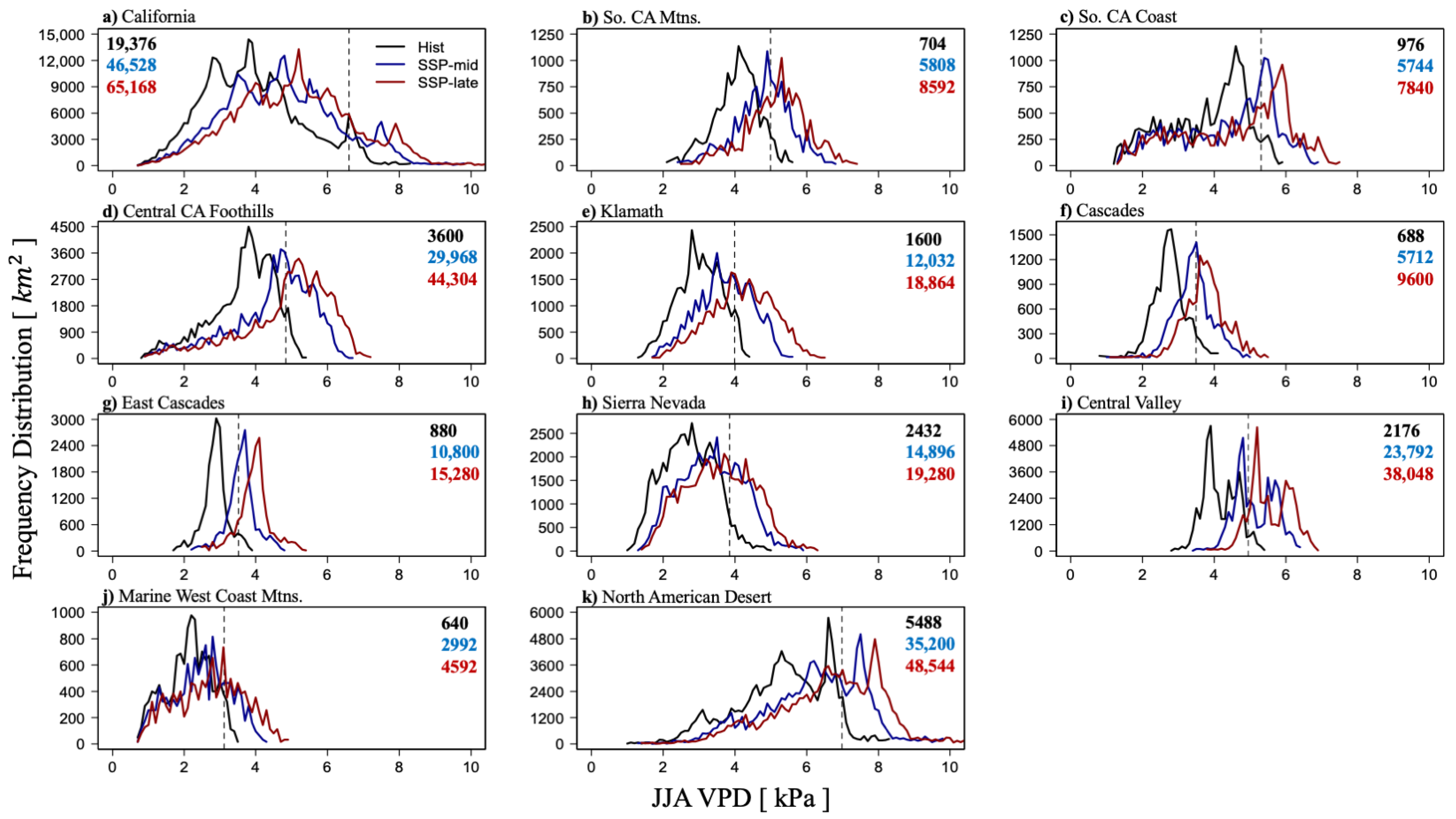
Ecoregion increases in JJA V P D 95 area were even more substantial than F W I 95 (Figure 9). The increase in VPD is so significant that the distribution of JJA VPD values shifts in a way that the peak VPD value in the mid- and late-century will exceed that of the historical 95th percentile threshold (Figure 9b–d,f,g,i,k). The largest increases in area exceeding V P D 95 occurred in the Central Valley and East Cascades, with a 17-fold increase, followed by the Cascades (13-fold), and the CCF and SCC (12-fold). The JJA V P D 95 percentile values ranged from 3.12 in the MWCM to 6.98 in the North American Desert, while the state-wide California JJA V P D 95 was 6.6.
The average projected area with extreme SON VPD was also large, implying that conditions in California will be conducive to wildfire for a minimum of half the year, extending the typical fire season into the fall, and contributing to the widespread desiccation of fuels. Unlike with patterns seen in the MWCM FWI values, V P D 95 area was projected to increase in the MWCM in both the JJA and SON by a factor of seven and nine, respectively (Figure 9j and Table 2). Additionally, the SON V P D 95 percentile values ranged from 2.01 in the East Cascades to 4.28 in the North American Desert, while the state-wide California JJA V P D 95 was 3.97.

3.5. Fire Weather Index Julian Day Climatologies

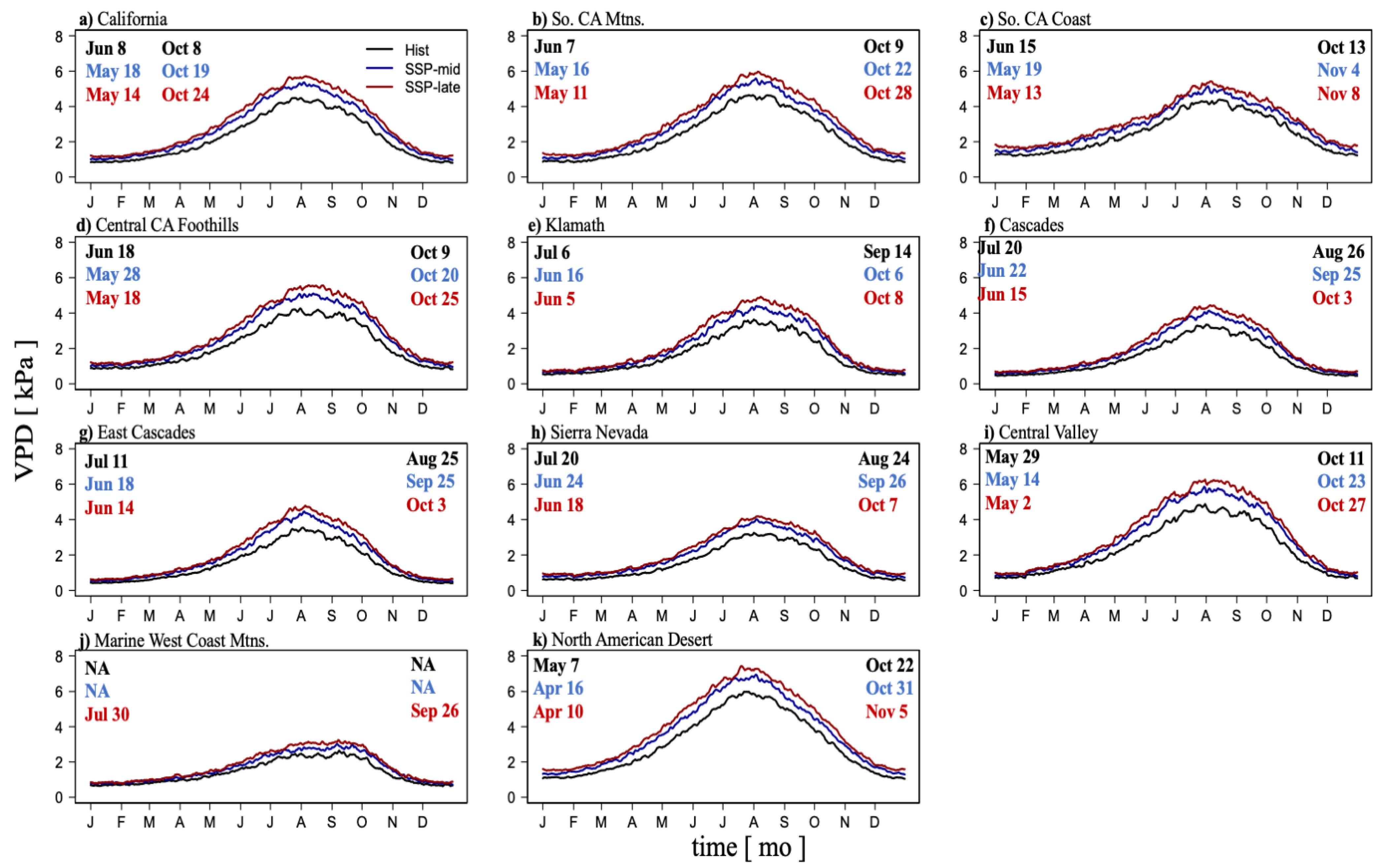
Julian day climatologies of VPD indicated an increase in peak VPD in the summer, as well as an earlier start and a delayed end to the fire season in all ecoregions of California (Figure 10). For example, by 2100, the average onset of high spring VPD (defined here as VPD ≥ 3) is a month or more earlier in the SCC, CCF, K, C, SN ecoregions. Furthermore, the decrease of VPD below the critical value is delayed by a month or more in the C, EC and SN. Our results indicated that climate change will likely increase summer and autumn average VPD and lengthen the amount of time each year that conditions favor large wildfires in California (Figure 10).
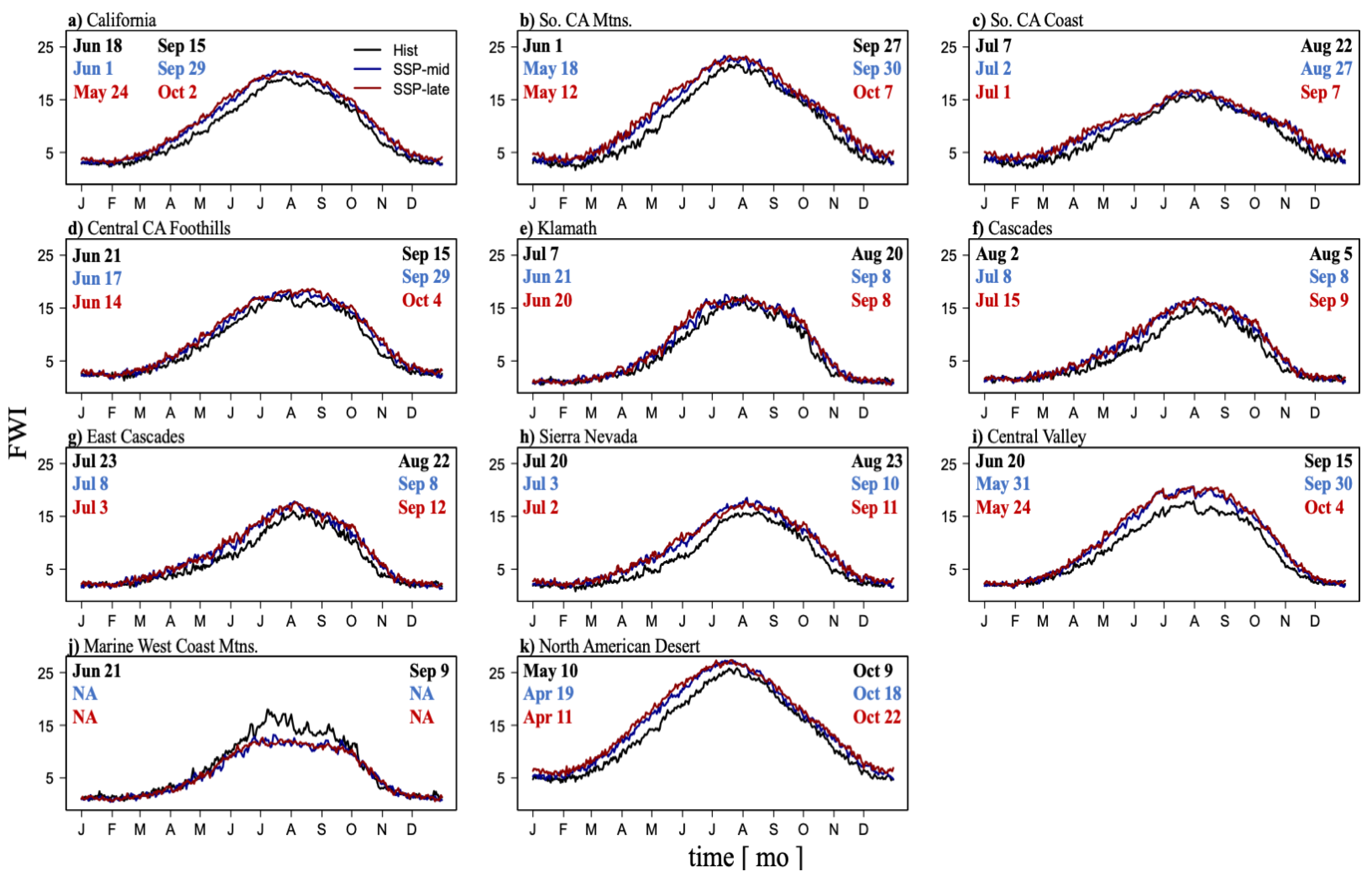
Julian day climatologies of FWI indicated that the average summer peak FWI value will increase, and the fire season, defined here by the onset of average FWI greater than 15, will begin earlier and end later in the mid- and late-century periods relative to the historic period. However, the effect of climate change on the growth of the fire season was greater for VPD than it was for FWI (Figure 11). The greatest impact was to the onset of the fire season, with late-century average FWI exceeding a value of 15 anywhere from 6 days (SCC) to one month (NAD) before the historical average.
Studies show that the role of temperature and humidity are strongest in FWI, with precipitation and wind speed playing important, but secondary roles [30,31]. However, our results indicated that the increase of VPD in the mid- and late-century periods was much greater than FWI, especially in the MWCM, which experienced a decrease in summer FWI, implying that precipitation and wind patterns can play a strong role in FWI trajectory (Figure 11j). However, the sensitivity of the FWI to incremental changes in input variables is outside the scope of this study.

4. Discussion

4.1. Extreme Fire Weather in California’s Future Will Become More Severe and Last Longer

California’s fire weather season length has increased in the past three decades due to increases in surface air temperature, decreases in relative humidity, and longer annual rain-free periods [30,32]. Our results provide further evidence that fire weather conditions conducive to large wildfires will become more extreme and extend later into the fall season in most areas of California by 2100 [3,30]. The peak effects of hot and dry summers will be extended by 30 days into late October and November. This timing will coincide with the Santa Ana wind season (which normally runs from October to March), as well as a projected delay in the onset of the rainy season—producing a high risk period during a time that has normally been outside of California’s typical “fire season” for emergency preparedness [30,33]. The catastrophic consequences of severe fire weather towards the end of the typical California fire season were seen in 2020, with the August Complex Fire (August 2020), SCU Lightning Complex (August 2020), Creek (September 2020), LNU Lightning Complex (August 2020), and the North Complex (August 2020)—together accounting for five of the 10 largest wildfires in California history [34,35]. In addition, the increase in land area experiencing extreme VPD and FWI expected by the end of the mid-century (2070) and late-century (2100) period, as well as the extension of the fire season late into the fall, will prime large portions of California for the spread of large wildfires, given an ignition (Figure 10 and Figure 11).

4.2. Climate Change Impacts on California Ecosystems

Several conceptual frameworks exist that seek to determine the biophysical controls on wildfire ignition and probability of spread. For example, wildfire has been shown to thrive in the middle of a continuum between aridity (dry) and productivity (wet) [36]. Similar to the way that plants have evolved traits that reflect biotic tradeoffs in favor of various survival strategies, wildfire regime is commonly controlled by the abundance and moisture content of fuels [37,38,39]. For example, the tropics experience large amounts of rainfall, have high biomass production, and contain the necessary fuels for large wildfires—however, they are rarely dry enough to burn [38,39]. On the other hand, where moisture is limited and biomass production is low, wildfire does not have the necessary fuel to spread. Therefore, wildfire would be most likely to occur and spread in ecosystems that are dry for sufficient periods of time so that vegetation becomes water-stressed, but wet enough to support enough biomass that provide continuous fuels such that large wildfires may burn. These environmental gradients impact all aspects of fire regime, including fire frequency, occurrence, intensity, severity, and total area burned [8,38,39]. This phenomenon implies that the projected impacts of climate change on temperature and atmospheric aridity will have a more significant effect on northern California forested ecoregions sensitive to extended dry periods than on the more consistently hot and dry southern California regions that are adapted to such conditions, and are more likely to lack the necessary abundance and continuity of fuel for large wildfires [9]. These climate-fire relationships are critical for the interpretation of our results, as the most substantial changes to the amount of area experiencing extreme fire weather (Figure 8 and Figure 9), as well as the time added to the onset and end of the fire season (Figure 10 and Figure 11), are projected to occur in forested northern California, where they could have the most dire implications for annual area burned throughout the 21st century.
In southern California, a large variety of topographies, vegetation types, climate regimes, and human populations contribute to a fire regime dominated by frequent wildfires. The precipitation season is confined to a few core months (Dec.–Mar.) with some rain occurring in the shoulder season of November and April, which in combination with the warm and dry summers, leads to an extended annual fire season [32]. In addition, annual Santa Ana winds advected from the eastern deserts towards the coast, move downslope at high speeds and increase the risk of severe wildfire during the fall season. Vegetation types are predominately herbaceous plants (chaparral), grasslands, shrubs, and patches of forest that recover relatively quickly following wildfire. The rapid regeneration of herbaceous fuels after wildfire are a factor in the frequent fire return interval throughout southern California (1–5 years) [40]. Studies show that the impacts of climate change on fire regime in southern California thus far are primarily a result of increasing temperatures and atmospheric aridity, as well as changing patterns of precipitation, that in turn influence the state of the environmental constraints on wildfire activity discussed above [41]. Compared to forested regions of northern California, fire regime in non-forested regions of southern California are less susceptible to shifts in moisture availability and more so to availability of fuel, however, these chaparral and grassland ecosystems are sensitive to rainfall patterns in the year or two prior to fire occurrence because the influx of moisture promotes the growth of vegetation [1,42]. Our results indicate that while the increases in land area experiencing extreme fire weather are smaller than in northern California, and the extension of the fire season is not as substantial, changes to southern California JJA and SON extreme fire weather, in succession, still have the potential to tax vegetation and fire-fighting resources.
Conceptual frameworks help to attribute controlling factors to different fire regimes, given the complex web of climate, human activity, topography, vegetation, hydrology, prior wildfire, fire suppression, and fire management, with their practically infinite combination. Our ecoregion specific results show a future consisting of more persistent extreme fire weather that occurs in a greater land surface area than in the past. Therefore, with the aid of climate-fire frameworks, we may deduce the range of impacts that this increase in aridity and fire potential may have on sensitive ecosystems. While northern and southern California ecoregion’s fire regimes are controlled by different factors, the simultaneous increasing trends in atmospheric aridity and fire potential indicate a future in which fire suppression and management resources throughout the state are stretched thin. In order to offset the dangers of extended fire seasons throughout much of California by 2100, alongside the expansion of the wildland urban interface, fire management must implement innovative combinations of new and existing strategies intended to limit the destruction of property and loss of life.

4.3. Limitations

Impact studies that utilize global climate model output generally require the use of many models, however, due to the recent release of CMIP6, limited availability of the fire weather variables required to perform the FWI and VPD calculations restricted our ability to increase the number of models used [43]. Despite this, the evaluation of the ensemble-mean of the three models chosen for this study showed good agreement with observational data. In addition, we acknowledge that all statistical downscaling methods are subject to issues of stationarity. To be clear, there are assumptions made regarding the application of historical climatic patterns to projected data, however, the thin plate spline and linear regression method employed here advantageously utilizes data surrounding each grid point in the calculation of its smoothed estimate. This interpolation technique works best with continuous data but it may be adapted to perform well with discontinuous climate variables such as precipitation, and to some extent wind speed. Additionally, it is important to consider the climate-wildfire-vegetation feedback when attempting to predict annual area burned, however, this work focuses on the impacts of climate on extreme fire weather, so the complex relationships among annual area burned, climate patterns, and vegetation distribution are outside the scope of this study [44]. Lastly, it should be noted that projected increases in California’s summer and fall VPD and FWI are not synonymous with a corresponding increase in annual area burned, as wildfire is inherently dependent on an ignition source and flammable vegetation [4].

5. Conclusions

We analyzed the impacts of climate change on extreme fire weather in ten different California ecoregions throughout historical, mid- and late-century periods using two prominent fire weather indices. Climate model output from three CMIP6 models were bias corrected and statistically downscaled using empirical quantile mapping in addition to a simple thin plate spline interpolation method. Historical average baselines for each index were calculated for each ecoregion and used to generate anomalies for 2041–2100. Relative change analysis indicates that FWI and VPD are projected to increase in all ecoregions, except the MWCM, which displayed a decrease in JJA and SON FWI in the mid- and late-century periods. In addition, the average daily 95th percentile value for the historical period (for each ecoregion) was implemented as a threshold in order to calculate the number of summer and fall extreme fire weather days, and to evaluate the spatial distribution of these changes. The frequency of 95th percentile days for JJA and SON VPD and FWI is projected to increase significantly in all ecoregions, except the MWCM, which shows a decline in FWI 95th percentile days. Furthermore, we analyzed the 30 year spatial average of each index and generated frequency distributions to investigate the average change in land area projected to experience extreme fire weather, relative to the historical benchmark. We found that JJA VPD land area exceeding the 95th percentile will increase by a factor of 2 and 17 in different ecoregions by the end of 2100. Lastly, Julian-day climatologies of each index were generated to assess the changing duration of a typical California fire season. We found that the window of extreme fire weather will expand into the spring and late autumn in all ecoregions (apart from the MWCM), extending the amount of time vegetation is exposed to increased atmospheric demand for moisture, and heightening the overall risk for the ignition and spread of large wildfire.
The ecoregion-level spatial scale adopted for this study increases the amount of local information, as well as the resolution with which fire and land managers can implement strategies and counter-measures when addressing issues related to climate change. The spatial downscaling algorithm tested and implemented in this study was computationally inexpensive (compared to dynamical downscaling) and may be readily applied to further climate change scenarios in other Mediterranean and temperate regions [13,15]. High resolution, daily meteorological data is not only useful for wildfire impact studies (and for investigating the post-fire environment), but can be implemented in the research of agricultural productivity, urban heat islands, hydrology, and human health. This intuitive, practical, and simple interpolation method will not only contribute to the improved understanding of the complexities of California’s climate-fire dynamics, but will provide the means for more efficiently obtaining climate model data of high spatial and temporal resolution.

Author Contributions

Conceptualization, D.E.R. and F.D.S.; methodology, D.E.R. and F.D.S.; software, D.E.R. and F.D.S.; validation, D.E.R.; formal analysis, D.E.R., F.D.S., D.S. and J.P.M.; investigation, D.E.R.; resources, D.E.R. and F.D.S.; data curation, D.E.R. and F.D.S.; writing—original draft preparation, D.E.R.; writing—review and editing, D.E.R., F.D.S., D.S. and J.P.M.; visualization, D.E.R., F.D.S. and J.P.M.; supervision, F.D.S., D.S. and J.P.M.; project administration, D.E.R. All authors have read and agreed to the published version of the manuscript.

Funding

This research received no external funding.

Institutional Review Board Statement

Not applicable.

Informed Consent Statement

Not applicable.

Data Availability Statement

The CMIP6 climate model output is publicly available through the Earth System Grid Federation at [doi:10.1016/j.future.2013.07.002]. Historical and Shared Socio-Economic Pathways (SSP585) data for the three models are available as follows: MIROC6 Historical at [https://doi.org/10.22033/ESGF/CMIP6.5603], MIROC6 SPP at [https://doi.org/10.22033/ESGF/CMIP6.5771], EC-Earth3 Historical at [https://doi.org/10.22033/ESGF/CMIP6.4700], EC-Earth3 SSP at [https://doi.org/10.22033/ESGF/CMIP6.4912], MRI-ESM2-0 Historical at [https://doi.org/10.22033/ESGF/CMIP6.6842], MRI-ESM2-0 SSP at [https://doi.org/10.22033/ESGF/CMIP6.6929]. NCEP North American Regional Reanalysis (NARR) data provided by the NOAA PSL, Boulder, Colorado, USA, from their website at https://psl.noaa.gov, accessed on 1 March 2022. TerraClimate observational data is publicly available at [doi:10.1038/sdata.2017.191]. Ecoregions of California are available through the United States Geological Survey at [http://dx.doi.org/10.3133/ofr20161021]. GridMET meteorological data is available at [https://doi.org/10.1002/joc.3413].

Acknowledgments

The authors would like to thank the NCAR Computational and Information System Laboratory and the SDSU Center for Earth System Analysis and Research for providing the computer facilities necessary for the completion of the study.

Conflicts of Interest

The authors declare no conflict of interest.

References

  1. Williams, A.P.; Abatzoglou, J.T.; Gershunov, A.; Guzman-Morales, J.; Bishop, D.A.; Balch, J.K.; Lettenmaier, D.P. Observed impacts of anthropogenic climate change on wildfire in California. Earth’s Future 2019, 7, 892–910. [Google Scholar] [CrossRef] [Green Version]
  2. Abatzoglou, J.T.; Williams, A.P. Impact of anthropogenic climate change on wildfire across western US forests. Proc. Natl. Acad. Sci. USA 2016, 113, 11770–11775. [Google Scholar] [CrossRef] [Green Version]
  3. Goss, M.; Swain, D.L.; Abatzoglou, J.T.; Sarhadi, A.; Kolden, C.A.; Williams, A.P.; Diffenbaugh, N.S. Climate change is increasing the likelihood of extreme autumn wildfire conditions across California. Environ. Res. Lett. 2020, 15, 9. [Google Scholar] [CrossRef] [Green Version]
  4. Keeley, J.E.; Syphard, A.D. Climate change and future fire regimes: Examples from California. Geosciences 2016, 6, 37. [Google Scholar] [CrossRef] [Green Version]
  5. Dong, L.; Leung, L.R.; Qian, Y.; Zou, Y.; Song, F.; Chen, X. Meteorological environments associated with California wildfires and their potential roles in wildfire changes during 1984–2017. J. Geophys. Res. Atmos. 2021, 126, 5. [Google Scholar] [CrossRef]
  6. Touma, D.; Stevenson, S.; Lehner, F.; Coats, S. Human-driven greenhouse gas and aerosol emissions cause distinct regional impacts on extreme fire weather. Nat. Commun. 2021, 12, 212. [Google Scholar] [CrossRef]
  7. Bonan, G.B. Forests and climate change: Forcings, feedbacks, and the climate benefits of forests. Science 2008, 320, 1444–1449. [Google Scholar] [CrossRef] [Green Version]
  8. Bradstock, R.A. A Biogeographic Model of Fire Regimes in Australia: Current and Future Implications: A Biogeographic Model of Fire in Australia. Glob. Ecol. Biogeogr. 2010, 19, 145–158. [Google Scholar] [CrossRef]
  9. McKenzie, D.; Littell, J.S. Climate change and the eco-hydrology of fire: Will area burned increase in a warming Western USA? Ecol. Appl. 2017, 27, 26–36. [Google Scholar] [CrossRef]
  10. Littell, J.S. Drought and fire in the Western USA: Is climate attribution enough? Curr. Clim. Chang. Rep. 2018, 4, 396–406. [Google Scholar] [CrossRef]
  11. Williams, J.W.; Jackson, S.T.; Kutzbach, J.E. Projected Distributions of Novel and Disappearing Climates by 2100 AD. Proc. Natl. Acad. Sci. USA 2007, 104, 5738–5742. [Google Scholar] [CrossRef] [PubMed] [Green Version]
  12. Johnstone, J.F.; Allen, C.D.; Franklin, J.F.; Frelich, L.E.; Harvey, B.J.; Higuera, P.E.; Mack, M.C.; Meentemeyer, R.K.; Metz, M.R.; Perry, G.L.W.; et al. Changing disturbance regimes, ecological memory, and forest resilience. Front. Ecol. Environ. 2016, 14, 369–378. [Google Scholar] [CrossRef]
  13. Abatzoglou, J.T.; Brown, T.J. A Comparison of Statistical Downscaling Methods Suited for Wildfire Applications: STATISTICAL DOWNSCALING FOR WILDFIRE APPLICATIONS. Int. J. Clim. 2012, 32, 772–780. [Google Scholar] [CrossRef]
  14. Li, H.; Sheffield, J.; Wood, E.F. Bias Correction of Monthly Precipitation and Temperature Fields from Intergovernmental Panel on Climate Change AR4 Models Using Equidistant Quantile Matching. J. Geophys. Res. 2010, 115, D10. [Google Scholar] [CrossRef]
  15. Zhang, L.; Xu, Y.; Meng, C.; Li, X.; Liu, H.; Wang, C. Comparison of Statistical and Dynamic Downscaling Techniques in Generating High-Resolution Temperatures in China from CMIP5 GCMs. J. Appl. Meteorol. Climatol. 2020, 59, 207–235. [Google Scholar] [CrossRef]
  16. van Wagner, C.E. The Development and Structure of the Canadian Forest Fire Weather Index System; Canadian Forest Service: Ottawa, ON, Canada, 1987. [Google Scholar]
  17. Lawson, B.D.; Armitage, O.B. Weather Guide for the Canadian Forest Fire Danger Rating System; Natural Resources Canada, Canadian Forest Service: Edmonton, AB, Canada, 2008. [Google Scholar]
  18. Lawson, B.D. Fire Weather Index—The Basis for Fire Danger Rating in British Columbia; Canadian Fisheries and Environment Canada, Canadian Forestry Service: Victoria, QC, Canada, 1977. [Google Scholar]
  19. Seager, R.; Hooks, A.; Williams, A.P.; Cook, B.; Nakamura, J.; Henderson, N. Climatology, Variability, and Trends in the U.S. Vapor Pressure Deficit, an Important Fire-Related Meteorological Quantity. J. Appl. Meteorol. Climatol. 2015, 54, 1121–1141. [Google Scholar] [CrossRef]
  20. Zhuang, Y.; Fu, R.; Santer, B.D.; Dickinson, R.E.; Hall, A. Quantifying contributions of natural variability and anthropogenic forcings on increased fire weather risk over the western United States. Proc. Natl. Acad. Sci. USA 2021, 118, e2111875118. [Google Scholar] [CrossRef]
  21. Level III and IV Ecoregions of Continental United States. Available online: https://www.epa.gov/eco-research/level-iii-and-iv-ecoregions-continental-united-states (accessed on 20 July 2021).
  22. Griffith, G.E.; Omernik, J.M.; Smith, D.W.; Cook, T.D.; Tallyn, E.; Moseley, K.; Johnson, C.B. Ecoregions of California. In U.S. Geological Survey Open-File Report 2016–1021; Western Geographic Science Center: Menlo Park, CA, USA, 2016. [Google Scholar]
  23. Abatzoglou, J.T. Development of gridded surface meteorological data for ecological applications and modelling. Int. J. Climatol. 2013, 33, 121–131. [Google Scholar] [CrossRef]
  24. Hancock, P.A.; Hutchinson, M.F. Spatial interpolation of large climate data sets using Bivariate Thin Plate Smoothing Splines. Environ. Model. Softw. 2006, 21, 1684–1694. [Google Scholar] [CrossRef]
  25. Hoar, T.; Nychka, D. Statistical Downscaling of the Community Climate System Model (CCSM) Monthly Temperature and Precipitation Projections [White Paper]. IMAGe/NCAR. Available online: http://www.gisclimatechange.org/Downscaling.pdf (accessed on 1 May 2022).
  26. Juras, J. Some common features of probability distributions for precipitation. Theor. Appl. Climatol. 1994, 49, 69–76. [Google Scholar] [CrossRef]
  27. Fu, G.; Viney, N.R.; Charles, S.P. Evaluation of various root transformations of daily precipitation amounts fitted with a normal distribution for Australia. Theor. Appl. Climatol. 2010, 99, 229–238. [Google Scholar] [CrossRef]
  28. Mesinger, F.; DiMego, G.; Kalnay, E.; Mitchell, K. North American Regional Reanalysis. Bull. Am. Meteorol. Soc. 2006, 87, 343–360. [Google Scholar] [CrossRef] [Green Version]
  29. Abatzoglou, J.T.; Dobrowski, S.Z.; Parks, S.A.; Hegewisch, K.C. Terraclimate, a high-resolution global dataset of monthly climate and climatic water balance from 1958–2015. Sci. Data 2018, 5, 170191. [Google Scholar] [CrossRef] [PubMed] [Green Version]
  30. Dong, C.; Williams, A.P.; Abatzoglou, J.T.; Lin, K.; Okin, G.S.; Gillespie, T.W.; Long, D.; Lin, Y.H.; Hall, A.; MacDonald, G.M. The season for large fires in Southern California is projected to lengthen in a changing climate. Commun. Earth Environ. 2022, 3, 22. [Google Scholar] [CrossRef]
  31. Jain, P.; Castellanos-Acuna, D.; Coogan, S.C.; Abatzoglou, J.T.; Flannigan, M.D. Observed increases in extreme fire weather driven by atmospheric humidity and temperature. Nat. Clim. Chang. 2022, 12, 63–70. [Google Scholar] [CrossRef]
  32. Jolly, W.M.; Cochrane, M.A.; Freeborn, P.H.; Holden, Z.A.; Brown, T.J.; Williamson, G.J.; Bowman, D.M. Climate-induced variations in global wildfire danger from 1979 to 2013. Nat. Commun. 2015, 6, 7537. [Google Scholar] [CrossRef] [Green Version]
  33. Swain, D.L. A shorter, sharper rainy season amplifies California wildfire risk. Geophys. Res. Lett. 2021, 48, e2021GL092843. [Google Scholar] [CrossRef]
  34. Top 20 Largest California Wildfires. 2022. Available online: https://www.fire.ca.gov/media/4jandlhh/top20_acres.pdf (accessed on 20 July 2021).
  35. Parks, S.A.; Parisien, M.A.; Miller, C.; Dobrowski, S.Z. Fire activity and severity in the western US vary along proxy gradients representing fuel amount and fuel moisture. PLoS ONE 2014, 9, e99699. [Google Scholar] [CrossRef]
  36. Bonan, G. Ecological Climatology: Concepts and Applications; Cambridge University Press: Cambridge, UK, 2015; ISBN 978-1107619050. [Google Scholar]
  37. Archibald, S.; Lehmann, C.E.R.; Gomez-Dans, J.L.; Bradstock, R.A. Defining Pyromes and Global Syndromes of Fire Regimes. Proc. Nat. Acad. Sci. USA 2013, 110, 6442–6447. [Google Scholar] [CrossRef] [Green Version]
  38. Meyn, A.; White, P.S.; Buhk, C.; Jentsch, A. Environmental Drivers of Large, Infrequent Wildfires: The Emerging Conceptual Model. Prog. Phys. Geogr. 2007, 31, 287–312. [Google Scholar] [CrossRef]
  39. Parks, S.A.; Miller, C.; Abatzoglou, J.T.; Holsinger, L.M.; Parisien, M.A.; Dobrowski, S.Z. How will climate change affect wildland fire severity in the western US? Environ. Res. Lett. 2016, 11, 035002. [Google Scholar] [CrossRef]
  40. Meng, R.; Dennison, P.E.; D’Antonio, C.M.; Moritz, M.A. Remote sensing analysis of vegetation recovery following short-interval fires in southern California shrublands. PLoS ONE 2014, 9, e110637. [Google Scholar] [CrossRef] [PubMed] [Green Version]
  41. Krawchuk, M.A.; Moritz, M.A. Constraints on Global Fire Activity Vary across a Resource Gradient. Ecology 2011, 92, 121–132. [Google Scholar] [CrossRef] [PubMed]
  42. Keeley, J.E.; Syphard, A.D. Twenty-first century California, USA, wildfires: Fuel-Dominated vs. wind-dominated fires. Fire Ecol. 2019, 15, 24. [Google Scholar] [CrossRef] [Green Version]
  43. Araya-Osses, D.; Casanueva, A.; Román-Figueroa, C.; Uribe, J.M.; Paneque, M. Climate change projections of temperature and precipitation in Chile based on statistical downscaling. Clim. Dyn. 2020, 54, 4309–4330. [Google Scholar] [CrossRef] [Green Version]
  44. Hurteau, M.D.; Liang, S.; Westerling, A.L.; Wiedinmyer, C. Vegetation-fire feedback reduces projected area burned under climate change. Sci. Rep. 2019, 9, 2838. [Google Scholar] [CrossRef]
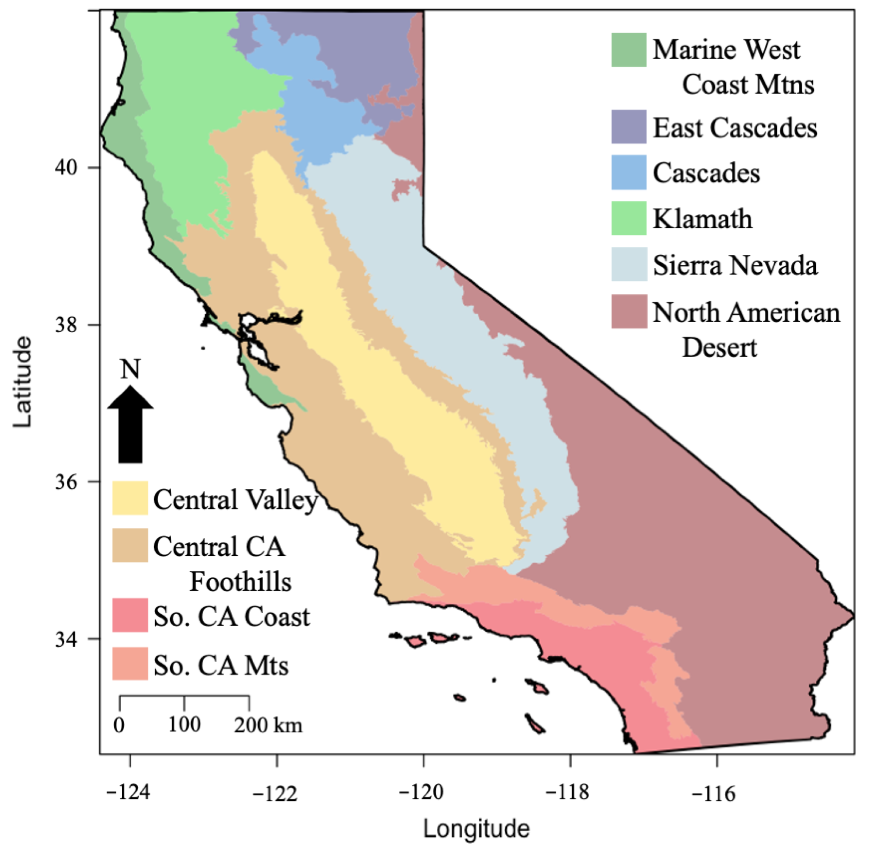
Figure 1. Ecoregions of California, including the southern California Mountains (SCM), southern California Coast (SCC), Central California foothills (CCF), Central Valley (CV), North American Desert (NAM), Sierra Nevada (SN), Klamath (K), Cascades (C), East Cascades (EC), Marine West Coast Mountains (MWCM), and North American Desert (NAD).
Fire 05 00177 g001
Figure 2. Average maximum temperature for 1979 (a) TerraClimate (b) Raw MIROC6 (c) BCSD Ensemble. Units: °C.
Fire 05 00177 g002
Figure 3. State-wide average monthly climatology (1979–2014) for the CMIP6 Raw and BCSD model ensembles. Observational data are an ensemble of NARR and TerraClimate. (a) Maximum temperature; (b) Daily Rainfall accumulation; (c) Minimum relative humidity; (d) 10 m wind speed.
Fire 05 00177 g003
Figure 4. Canadian Fire Weather Index anomaly relative to the historical period of 1981–2010. Solid black line represents the summer season of June, July, and August, while the solid red line represents the fall season of September, October, November. The dashed vertical black line represents the end of the historical period, while the dashed vertical blue and red lines represent the breaks between the mid- and late-century periods, respectively. The black and red text within the figure is the relative change (%) for the mid- and late-century periods (relative to the historical period) in the JJA and SON seasons, respectively. (a) California; (b) Southern California Mountains; (c) Southern California Coast; (d) Central California Foothills; (e) Klamath; (f) Cascades; (g) East Cascades; (h) Sierra Nevada; (i) Central Valley; (j) Marine West Coast Mountains; (k) North American Desert.
Fire 05 00177 g004
Figure 5. Vapor pressure deficit anomaly relative to the historical period of 1981–2010. Solid black line represents the summer season of June, July, and August, while the solid red line represents the fall season of September, October, November. The dashed vertical black line represents the end of the historical period, while the dashed vertical blue and red lines represent the breaks between the mid- and late-century periods, respectively. The black and red text within the figure is the relative change (%) for the mid- and late-century periods (relative to the historical period) in the JJA and SON seasons, respectively. (a) California; (b) Southern California Mountains; (c) Southern California Coast; (d) Central California Foothills; (e) Klamath; (f) Cascades; (g) East Cascades; (h) Sierra Nevada; (i) Central Valley; (j) Marine West Coast Mountains; (k) North American Desert. Units: kPa.
Fire 05 00177 g005
Figure 6. Average frequency (in days/yr) with which VPD and FWI exceed the ecoregion-specific daily average JJA 95th percentile in the mid-century (left) and late-century (right) relative to the historic period. Higher values indicate more JJA days each year that exceeded the 95th percentile. (a,b) Vapor pressure deficit (c,d) Fire Weather Index.
Fire 05 00177 g006
Figure 7. Average frequency (in days/yr) with which VPD and FWI exceed the ecoregion specific daily average SON 95th percentile in the mid-century (left) and late-century (right) relative to the historic period. Higher values indicate more SON days that exceeded the 95th percentile. (a,b) Vapor pressure deficit (c,d) Fire Weather Index.
Fire 05 00177 g007
Figure 8. Frequency distribution depicting the area experiencing particular JJA FWI values. The dashed line represents the ecoregion specific 30 year average spatial 95th percentile value. The black, blue, and red lines represent the historical, mid-century, and late-century time periods, respectively. The color-coded text are areal units ( km 2 ) experiencing greater than the 95th percentile value for that ecoregion. (a) California; (b) Southern California Mountains; (c) Southern California Coast; (d) Central California Foothills; (e) Klamath; (f) Cascades; (g) East Cascades; (h) Sierra Nevada; (i) Central Valley; (j) Marine West Coast Mountains; (k) North American Desert.
Fire 05 00177 g008
Figure 9. Frequency distribution depicting the area experiencing particular JJA VPD values. The dashed line represents the ecoregion specific 30 year average spatial 95th percentile value. The black, blue, and red lines represent the historical, mid-century, and late-century time periods, respectively. The color-coded text are areal units ( km 2 ) experiencing greater than the 95th percentile value for that ecoregion. (a) California; (b) Southern California Mountains; (c) Southern California Coast; (d) Central California Foothills; (e) Klamath; (f) Cascades; (g) East Cascades; (h) Sierra Nevada; (i) Central Valley; (j) Marine West Coast Mountains; (k) North American Desert.
Fire 05 00177 g009
Figure 10. Thirty-year average Julian day VPD value by ecoregion. The black, blue, and red lines represent the historical, mid-century, and late-century averages, respectively. The color-coded text shows the average date for each respective time period that VPD exceeds (left) and falls below (right) a value of 3. (a) California; (b) Southern California Mountains; (c) Southern California Coast; (d) Central California Foothills; (e) Klamath; (f) Cascades; (g) East Cascades; (h) Sierra Nevada; (i) Central Valley; (j) Marine West Coast Mountains; (k) North American Desert. Units: kPa.
Fire 05 00177 g010
Figure 11. Thirty-year average Julian day Fire Weather Index value by ecoregion. The black, blue, and red lines represent the historical, mid-century, and late-century averages, respectively. The color-coded text shows the average date for each respective time period that FWI exceeds (left) and falls below (right) a value of 15. (a) California; (b) Southern California Mountains; (c) Southern California Coast; (d) Central California Foothills; (e) Klamath; (f) Cascades; (g) East Cascades; (h) Sierra Nevada; (i) Central Valley; (j) Marine West Coast Mountains; (k) North American Desert.
Fire 05 00177 g011
Table 1. Spatial statistics (i.e., sCor) evaluating a 36 year average historical period (1979–2014) of the raw CMIP model ensemble and the bias-corrected and spatially downscaled CMIP model ensemble, against the NARR/TerraClimate validation dataset. Temporal statistics (i.e., tCor) are based on 36 years of monthly averages. Standard deviation is shown in parentheses. Spatial correlations are significant at p < 0.001.
CMIP RawCMIP BCSD
Max Temperature
sCor/tCor0.82/0.970.95/0.97
sBias/tBias0.74 (±2.76)/−0.76 (±0.8)1.17 (±1.62)/−1.18 (±0.77)
sRMSE/tRMSE2.11 (±1.93)/2.45 (±0.46)1.55 (±1.26)/2.22 (±0.49)
Daily Precip Acc
sCor/tCor0.88/0.610.88/0.61
sBias/tBias0.96 (±0.55)/−0.93 (±0.57)0.42 (±1.19)/−0.42 (±0.54)
sRMSE/tRMSE0.97 (±0.52)/1.97 (±0.55)0.64 (±1.08)/1.64 (±0.44)
Min. Rel Hum
sCor/tCor0.79/0.860.87/0.86
sBias/tBias10.75 (±8.03)/−13.72 (±3.98)−8.3 (±6.91)/5.51 (±3.83)
sRMSE/tRMSE12.18 (±5.62)/16.57 (±3.41)8.48 (±6.69)/12.58 (±3.92)
Wind Speed
sCor/tCor0.3/0.470.7/0.51
sBias/tBias0.67 (±0.68)/−0.69 (±0.09)0.29 (±0.65)/−0.29 (±0.09)
sRMSE/tRMSE0.8 (±0.51)/0.88 (±0.08)0.51 (±0.5)/0.51 (±0.08)
Table 2. Ecoregion average number of V P D 95 and F W I 95 days per year in each time period.
CASCMSCCCCFKCECSNCVMWCMNAD
JJA
FWI
Hist25102414119813101215
Mid331931241219172329326
Late342032261320182231329
VPD
Hist23121815111071781822
Mid3933333931333335343143
Late4743394944464742484052
SON
FWI
Hist1281396768778
Mid16111613913121415311
Late18141815915151617314
VPD
Hist1291197761061010
Mid2118192118181720191919
Late2726262725252526272426
Table 3. The extent of each ecoregion experiencing SON FWI and VPD greater than the 95th percentile. Calculated from the ecoregion 30 year average. Units: km 2 .
SONCASCMSCCCCFKCECSNCVMWCMNAD
FWI
Hist19,92067297637281648656896233621446565328
Mid14,5523088534411,664368050404320920018,3688019,840
Late64,6724848678416,00040165840582412,04823,5206432,784
VPD
Hist18,99276894436321552672848240022886565520
Mid54,1926656875227,42415,168572811,13614,99227,632436829,552
Late109,344952011,50446,40021,712956815,79222,09642,048604849,712
Publisher’s Note: MDPI stays neutral with regard to jurisdictional claims in published maps and institutional affiliations.