Numerical Study of the Effectiveness of a Firebreak in a Savanna Area and the Sizing Rules by an Optimised Fire Propagation Model

Abstract

Firebreaks are one of the techniques used to fight bushfires in Côte d’Ivoire. Their objective is to prevent the progression of fire and to protect sensitive sites. In this paper, a parametric study on the effectiveness of a firebreak in a savanna area is conducted using a fire spread model. The ability of the model to conduct this study was tested by an empirical model based on fire experiments in the Australian savanna. An agreement was found between the results predicted by our model and those of the empirical model. The parametric study conducted on the effectiveness of firebreaks indicated that a firebreak thickness equal to twice the flame length was effective. For bushfire control in Côte d’Ivoire, a firebreak with a minimum thickness of 8 m could stop the fire despite the slope of the land and the wind speed.

1. Introduction

According to SODEFOR, the state-owned company in charge of the development and management of natural forests and plantations in Côte d’Ivoire, the northern half of the country (about 160,000 km²) is affected by devastating and uncontrollable bushfires [1]. Between 1990 and 2004, 4650 hectares of forest plantations were destroyed by bushfires, 122 lives were lost, and 356 villages were burnt. Each year, between December and February, Côte d’Ivoire experiences a peak in bushfires that devastate hundreds of thousands of hectares of land suitable for agriculture. In 2016 (a drought year), bushfires destroyed more than 15,000 hectares of agricultural crops, 11,000 hectares of forest, and 200 huts in 10 villages and caused the death of 17 people. The damage was estimated at 204 billion FCFA (USD 363 million) [2]. With the increase in temperature in Côte d’Ivoire [2], there are fears that the number of areas affected by bushfires will increase and that they will intensify. It is therefore of utmost importance to manage fires properly, based on thorough multidisciplinary scientific research. This implies a regular review of management approaches and the exploration of new techniques [3,4,5,6].

The consequences of global warming have led several African countries to develop policies to combat vegetation fires. In Côte d’Ivoire, bushfires are the most frequent, especially in the forest–habitat interface. To combat the negative effects of bushfires, awareness campaigns are conducted among the population to avoid starting these fires in the dry season (late fires), whether for hunting or for cultivation. Village monitoring committees have been set up [1]. Firebreaks, which reduce the fuel load in strategically important areas, are one of the most widely used techniques to protect villages, plantations, and other sensitive sites from bushfires. The concept of “fuel breaks” is related to breaks of a few metres to 300 m in width, while “firebreaks” are used for breaks of a few metres [7,8].

Although this control technique has been popularised in many parts of Côte d’Ivoire, few quantitative studies have been reported. The fact that villages, plantations, and forests continue to be burnt by bushfires suggests that there is a need to better understand firebreak design. The questions we ask are: what factors determine the thickness of the firebreak in the savanna zone, and how thick the firebreak should be to stop a bushfire.

Models exist for the design of firebreak [9,10]. From experiments conducted in the Northern Territory of Australia in July–August 1986 [11,12], Wilson [9] developed an equation to predict firebreak failure. He estimated the probability of firebreak failure as a function of the intensity of the fire front, the width of the firebreak, and the presence or absence of trees within 20 m of the firebreak. This empirical model does not take into account wind speed and slope. Butler et al. (1998) developed a model based on flame radiation [10]. It does not take into account heat transfer by convection, which in some cases can become the dominant mode of heat transfer [13,14].

In this paper, we determine, from simulations carried out after variation of some essential fire parameters, the thickness necessary for a firebreak not to be breached by a bushfire. The tool used is a 2D mathematical bushfire spread model tested on several fires [15,16,17,18]. This model is able to estimate the effective thickness of a firebreak as a function of flame height, wind speed in savanna areas, and slope of the terrain. The main heat transfer modes are taken into account, namely radiation and convection.

To evaluate the prediction of our model, the probability of a firebreak being breached from Wilson’s (1988) logistic equation is compared to the predictions of our model. After this comparison, we study the effectiveness of the firebreaks and establish rules for their sizing.

It should be noted that “brandons”, which are flaming debris projected in front of the fire front by the wind, are not taken into account in this study. Similarly, there are no trees in the vicinity of the firebreaks.

2. Model Description

2.1. Physical Modelling

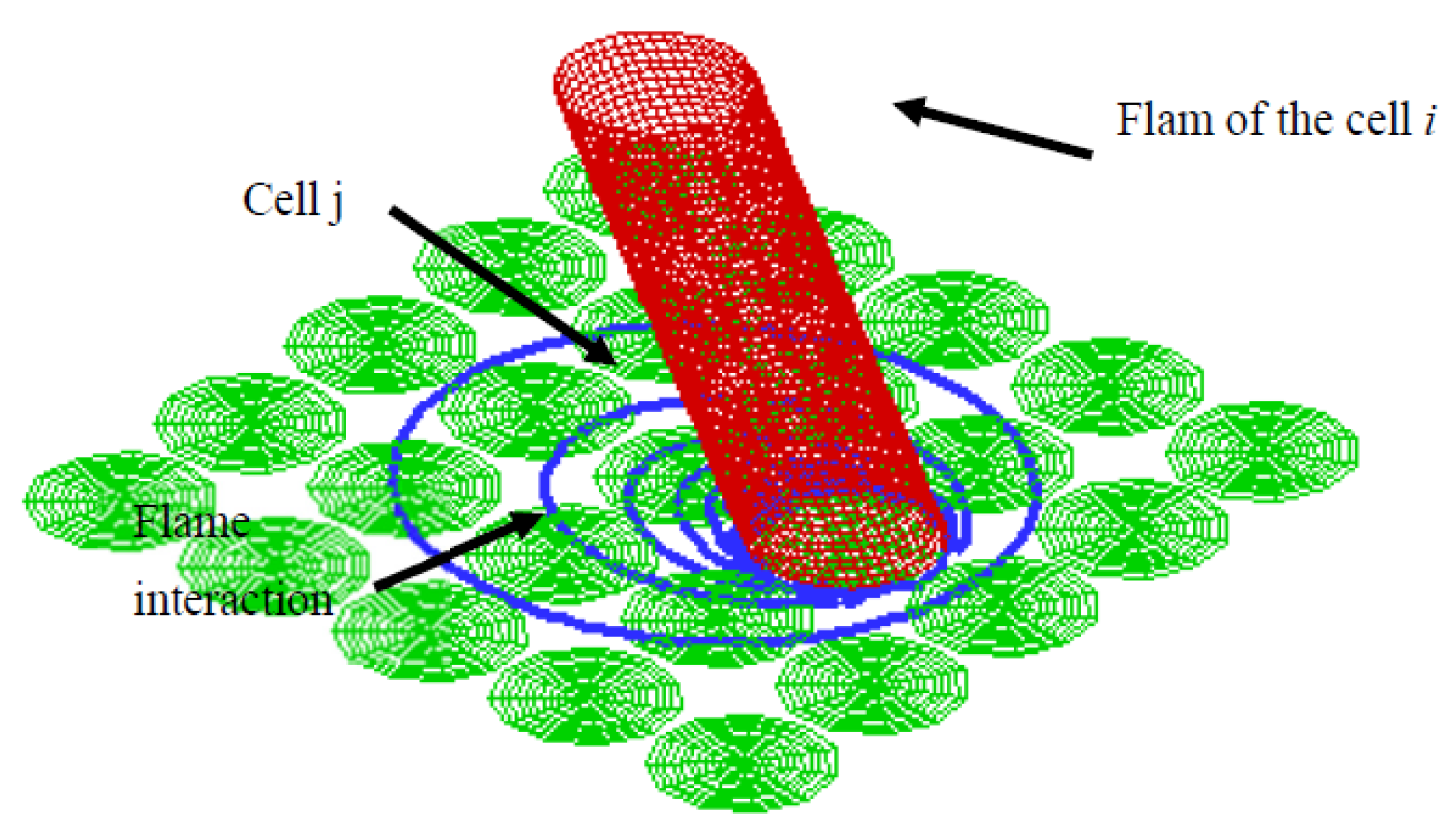
The present model is constructed from a regular two-dimensional array of equal-sized cells (Figure 1). Each fuel cell j is assumed to have a cylindrical shape with height $H_j$ and diameter $dia{m}_j$. The flame is assumed to be cylindrical in shape and is located on the burning cell i. Cell j, which is in the interaction zone of burning cell i, receives energy by radiation and convection. This received energy is used to raise the temperature of cell j to the boiling temperature of water (373 K).

The flame is assumed to be cylindrical and is shown in red. The fuel layer cells are in green, and the blue contours represent the flame interaction zone as a function of the view factor.

At this temperature, the water in cell j evaporates thanks to the energy received. After the evaporation of the water, the temperature of the cell increases to the ignition temperature ($T_{ign}=500 \mathrm{K}$). Some of this energy is lost to the surrounding environment by radiation. When the healthy cell j is in the interaction zone of several burning cells, it receives energy from all these burning cells. The reader interested in this model will find more details in [16,17,18].

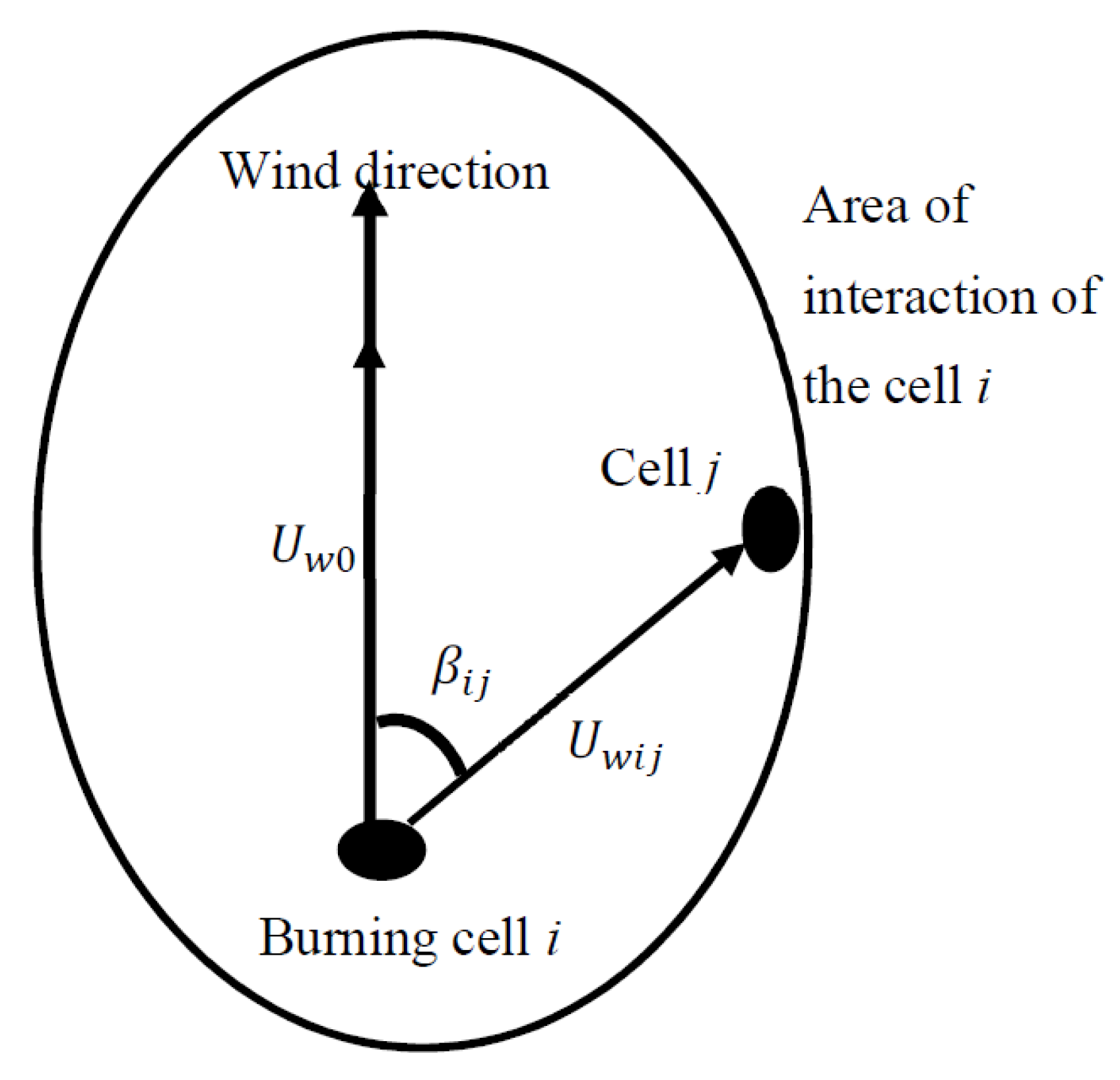
The convective heat flux received is maximum in the wind direction. The calculation of the convective heat flux received by cell j from the burning cell i is based on the wind speed $U_{wij}$ (Figure 2). $U_{w0}$ represents the wind intensity in the wind direction.

2.2. Mathematical Modelling

The heat flux $q_{ij}$ emitted by radiation and convection from the burning cell i and received by the healthy cell j is [13,16,19]

$$q_{ij}=\underset{surface\\ radiation}{\underbrace{\frac{a_{fb}{\epsilon }_{fl}\sigma T_{fl}^4}{H_j}{F}_{ij}}}+\underset{\begin{array}{c}internal\\ radiation\end{array}}{\underbrace{0.25A_{fb}{\epsilon }_b\sigma T_b^{4}exp\left(-0.25A_{fb}{d}_{ij}\right)}}+\underset{\begin{array}{c}surface\\ convection\end{array}}{\underbrace{\frac{0.565k_{fl}R{e}_{d_{ij}}^{1/2}P{r}^{1/2}}{d_{ij}{H}_j}\left(T_{fl}-T_j\right)exp\left(-0.3d_{ij}/L_{fl}\right)}}+\underset{\begin{array}{c}internal\\ convection\end{array}}{\underbrace{\frac{0.911A_{fb}{k}_{b}R{e}_D^{0.385}P{r}^{1/3}}{dia{m}_j}\left(T_b-T_j\right)exp\left(-0.25A_{fb}{d}_{ij}\right)}}-\underset{\begin{array}{c}radiative\\ loss\end{array}}{\underbrace{\frac{{\epsilon }_{fb}\sigma \left(T_j^4-T_{\infty }^4\right)}{H_j}}} .$$

(1)

where${\epsilon }_{fl}$ is the emissivity of the flame, $L_{fl}$ is the length of the flame, $a_{fb}$ is the absorption coefficient of the fuel, and $\sigma$ is the Stephan–Boltzmann constant; $F_{ij}$ is the radiant view factor between the flame (cell i) and the cell j, ${\epsilon }_b$ is the emissivity and $k_b$ is the thermal conductivity of the embers. $A_{fb}$ is the specific surface area of the fuel and $T_b$ is the temperature of the embers, ${\epsilon }_{fb}$ is the emissivity of the fuel layer, $d_{ij}$ is the distance between cell i and cell j; Pr is the Prandtl number and $d_{ij}$ is the distance between cells i and j. The diameter of the fuel located on cell j is denoted $dia{m}_j$. $T_{fl}$ and $T_j$ are the temperature of the flame and that of cell j. Reynolds numbers $R{e}_{d_{ij}}$ and $R{e}_{D_j }$ are given by

$$R{e}_{d_{ij}}=\frac{U_{wij}{d}_{ij}}{{\nu }_g} \mathrm{et} R{e}_{D_i}=\frac{U_{fb}{D}_i}{{\nu }_g}.$$

(2)

The wind intensity $U_{wij}$ in directions i and j is expressed as $U_{wij}=U_{w0}\cos {\beta }_{ij}$ and the wind intensity $U_{fb}$ inside the fuel layer is given by $U_{fb}=\left(1-{\varphi }_j\right)U_{wij}$. ${\varphi }_j$ is the volume fraction of the fuel located on cell j. The thermal conductivity of the flame $k_{fl}$ and its kinematic viscosity ${\nu }_g$ are assumed to be those of air at the flame temperature. The total energy $q_j$ of cell j is:

$$q_j=\left\{\begin{array}{c}{\rho }_j{C}_{pj}{\varphi }_j\frac{d{T}_j\left(t\right)}{dt}, for T_j\ne 373K\\ -{\rho }_j{h}_{vap}{\varphi }_j\frac{d{W}_j\left(t\right)}{dt}, for T_j=373K\end{array}\right.$$

(3)

where $W_j$ is the mass fraction of water in cell j; ${\rho }_j$ is the density of the fuel particle and $C_{pj}$ is its specific heat. $h_{vap}$ is the specific enthalpy of change of water from liquid to gas at 373 K. According to the law of conservation of energy, $q_j$ is also equal to

$$q_j={\displaystyle \sum }_{i=1}^{N_j}{q}_{ij},$$

(4)

where $N_j$ represents the number of burning cells interacting with cell j and $T_j$ is its temperature. Taking into account Equations (1), (3), and (4), for $T_j\ne 373 \mathrm{K}$, we obtain the following Cauchy problem:

$$\left\{\begin{array}{c}\frac{d{T}_j\left(t\right)}{dt}={\displaystyle {\displaystyle \sum }_{i=1}^{N_j}}{S}_{ij}\left(T_j\left(t\right)\right)\\ T_j\left(0\right)=T_{\infty }\end{array}\right.$$

(5)

${\displaystyle \sum }_{i=1}^{N_j}{S}_{ij}\left(T_j\left(t\right)\right) et T_j\left(t\right)$ are functions such as:

$$\begin{array}{c}{{\displaystyle \sum }}_{i=1}^{N_j}{S}_{ij}\left(T_j\left(t\right)\right): \left[T_{\infty },T_{fl}\right]\times \left[t_0,t_{max}\right]\to ℝ\\ \left(T_j,t\right)\to {{\displaystyle \sum }}_{i=1}^{N_j}\frac{1}{{\rho }_j{C}_{pj}{\varphi }_j}{q}_{ij}\end{array}$$

(6)

2.3. Existence and Uniqueness of the Solution of the Model Equation (5)

The Cauchy problem (5) admits a unique solution if, the function ${\displaystyle \sum }_{i=1}^{N_j}{S}_{ij}\left(T_j\left(t\right)\right)$ is Lipchitzian. In this section, we will show that the function ${\displaystyle \sum }_{i=1}^{N_j}{S}_{ij}\left(T_j\left(t\right)\right)$ is Lipchitzian in $T_j\left(t\right)$ on $\left[T_{\infty },T_{fl}\left]\times \right[t_0,t_{max}\right]$. Let the expression for ${\displaystyle \sum }_{i=1}^{N_j}{S}_{ij}\left(T_j\left(t\right)\right)$:

$${\displaystyle \sum }_{i=1}^{N_j}{S}_{ij}\left(T_j\left(t\right)\right)=q_j^{SR}+q_j^{IR}+K_1\left(T_{fl}-T_j\right)+K_2\left(T_b-T_j\right)-K_3\left(T_j^4-T_{\infty }^4\right)$$

(7)

With:

$$\left\{\begin{array}{c}{q}_j^{SR}={\displaystyle {\displaystyle \sum }_{i=1}^{N_j}}\left(\frac{a_{fb}{\epsilon }_{fl}\sigma T_{fl}^4}{H_j}{F}_{ij}\right)\\ q_j^{IR}={\displaystyle {\displaystyle \sum }_{i=1}^{N_j}}\left(0.25A_{fb}{\epsilon }_b\sigma T_b^{4}exp\left(-0.25A_{fb}{d}_{ij}\right)\right)\\ K_1={\displaystyle {\displaystyle \sum }_{i=1}^{N_j}}\left(\frac{0.565k_{fl}R{e}_{d_{ij}}^{1/2}P{r}^{1/2}}{d_{ij}{H}_j}exp\left(-0.3d_{ij}/L_{fl}\right){\beta }_{ij}\right)\\ K_2={\displaystyle {\displaystyle \sum }_{i=1}^{N_j}}\left(\frac{0.911A_{fb}{k}_{b}R{e}_D^{0.385}P{r}^{1/3}}{dia{m}_j}exp\left(-0.25A_{fb}{d}_{ij}\right){\beta }_{ij}\right)\\ K_3=\frac{{\epsilon }_{fb}\sigma }{H_j}\end{array}\right.$$

(8)

We then have:

$$\left|{\displaystyle \sum }_{i=1}^{N_j}{S}_{ij}\left(T_{1j}\left(t\right)\right)-{\displaystyle \sum }_{i=1}^{N_j}{S}_{ij}\left(T_{2j}\left(t\right)\right)\right|=\left|K_1\left(T_{2j}-T_{1j}\right)+K_2\left(T_{2j}-T_{1j}\right)+K_3\left(T_{2j}^4-T_{1j}^4\right)\right|$$

After some calculations, we obtain

$$\left|{\displaystyle \sum }_{i=1}^{N_j}{S}_{ij}\left(T_{1j}\left(t\right)\right)-{\displaystyle \sum }_{i=1}^{N_j}{S}_{ij}\left(T_{2j}\left(t\right)\right)\right|\le \left(K_1+K_2+4K_3{T}_{fl}^3\right)\left|T_{2j}-T_{1j}\right|.$$

(9)

The function ${\displaystyle \sum }_{i=1}^{N_j}{S}_{ij}\left(T_j\left(t\right)\right)$ is therefore Lipchitzian with a ratio $L=K_1+K_2+4K_3{T}_{fl}^3$. Therefore, Equation (5) has a unique solution.

2.4. Solving the Equation by the Runge–Kutta Method of Order 4

The Runge–Kutta 4th order method for solving the differential equation

$$\left\{\begin{array}{c}{y}^{\prime }\left(t\right)=f\left(t,y\left(t\right)\right)\\ y\left(0\right)=y_0\end{array}\right.$$

consists in calculating the sequence $\left(y^n\right)$ of approximations of the function $y$ as follows:

$$\left\{\begin{array}{c}{k}_1=\Delta t.f\left(t_n,y^n\right)\\ k_2=\Delta t.f\left(t_n+\frac{\Delta t}{2},y^n+\frac{k_1}{2}\right)\\ k_3=\Delta t.f\left(t_n+\frac{\Delta t}{2},y^n+\frac{k_2}{2}\right)\\ k_4=\Delta t.f\left(t_n+\Delta t,y^n+k_3\right)\\ y^{n+1}=y^n+\frac{k_1}{\begin{array}{c}6\\ \end{array}}+\frac{k_2}{3}+\frac{k_3}{3}+\frac{k_4}{6}\end{array}\right.$$

(10)

where $\Delta t$ is the time step and $f\left(t,y\left(t\right)\right)$ a function defined for $t\ge 0$ and $y\left(t\right)\in ℝ$.

To solve Equation (5), a discretization by the Runge–Kutta method of order 4 is performed, we obtain:

$$\left\{\begin{array}{c}\Delta T_j^{\left(n-1,1\right)}=\Delta t{\displaystyle {\displaystyle \sum }_{i=1}^{N_j}}{S}_{ij}\left(t_n,T_j^{\left(n-1\right)}\right)\\ \Delta T_j^{\left(n-1,2\right)}=\Delta t{\displaystyle {\displaystyle \sum }_{i=1}^{N_j}}{S}_{ij}\left(t_n+\frac{\Delta t}{2},T_j^{\left(n-1\right)}+\frac{\Delta T_j^{\left(n-1,1\right)}}{2}\right)\\ \Delta T_j^{\left(n-1,3\right)}=\Delta t{\displaystyle {\displaystyle \sum }_{i=1}^{N_j}}{S}_{ij}\left(t_n+\frac{\Delta t}{2},T_j^{\left(n-1\right)}+\frac{\Delta T_j^{\left(n-1,2\right)}}{2}\right)\\ \Delta T_j^{\left(n-1,4\right)}=\Delta t{\displaystyle {\displaystyle \sum }_{i=1}^{N_j}}{S}_{ij}\left(t_n+\Delta t,T_j^{\left(n-1\right)}+\Delta T_j^{\left(n-1,3\right)}\right)\\ T_j^{\left(n\right)}=T_j^{\left(n-1\right)}+\frac{\Delta T_j^{\left(n-1,1\right)}}{6}+\frac{\Delta T_j^{\left(n-1,2\right)}}{3}+\frac{\Delta T_j^{\left(n-1,3\right)}}{3}+\frac{\Delta T_j^{\left(n-1,4\right)}}{6}\end{array}\right.$$

(11)

In (11), $T_j^{\left(n-1\right)}$ is the approximation of the temperature of cell j at times $t_{n-1}$ and $\Delta t$ is the constant time step of discretization.

Equation (11) is used to calculate the temperature of cell j as a function of time. To reduce the calculation time, cells j that are not in the interaction zone of a burning site at the time of the calculation are not taken into account. When the temperature of cell j reaches the ignition temperature $T_{ign}$ ($=500 \mathrm{K}$), cell j is on fire and contributes to the thermal degradation of the cells in its interaction zone.

2.5. Calibration of Model Parameters

The model depends on several parameters that are difficult to measure in the field or to assess accurately. Apart from the input data, the present model depends on seven parameters that have an impact on the model results. These parameters are given in

Table 1. Parameter values.

Parameters	Initial Values
Fuel absorption coefficient $a_{fb}$ (-)	0.6
Flame temperature $T_{fl} \left(K\right)$	1083
Emissivity of embers ${\epsilon }_b$ (-)	1
Emissivity of the fuel layer ${\epsilon }_{fb}$ (-)	0.6
Flame conductivity $k_{fl} \left(\mathrm{W}.{\mathrm{m}}^{-1}.{\mathrm{K}}^{-1}\right)$	0.0707
Conductivity of embers $k_b \left(\mathrm{W}.{\mathrm{m}}^{-1}.{\mathrm{K}}^{-1}\right)$	0.0454
Temperature of embers $T_b \left(K\right)$	561

.

To improve the prediction of the model, we will calibrate these parameters. Let $\theta$ be the vector of parameters, we have

$$\theta ={\left(a_{fb},T_{fl},{\epsilon }_b,{\epsilon }_{fb},k_{fl},k_b,T_b\right)}^T ϵ \mathsf{\Omega }\subset {ℝ}^7.$$

(12)

$$\mathsf{\Omega }=\left[0.3;1\right]\times \left[700;1200\right]\times \left[0.1;1\right]\times \left[0.1;1\right]\times \left[0.0371;0.225\right]\times \left[0.0205;0.105\right]\times \left[500;700\right].$$

(13)

The expression for $S_{ij}\left(T_j\left(t\right)\right)$, shows that it depends not only on the temperature $T_j\left(t\right)$, but also on the parameters listed in Table 1.

Let us rewrite $S_{ij}\left(T_j\left(t\right)\right)$ more explicitly in terms of $\theta$ and $T_j\left(t\right)$

$$S_{ij}\left(\theta ,T_j\left(t\right)\right)=\underset{\begin{array}{c}surface\\ radiation\end{array}}{\underbrace{A_{ij}{\theta }_1{\theta }_2^4}}+\underset{\begin{array}{c}internal\\ radiation\end{array}}{\underbrace{B_{ij}{\theta }_3{\theta }_7^4}}+\underset{\begin{array}{c}surface\\ convection\end{array}}{\underbrace{D_{ij}{\theta }_5\left({\theta }_2-T_j\left(t\right)\right)}}+\underset{\begin{array}{c}internal\\ convection\end{array}}{\underbrace{E_{ij}{\theta }_6\left({\theta }_7-T_j\left(t\right)\right)}}-\underset{\begin{array}{c}radiative\\ loss\end{array}}{\underbrace{C_{ij}{\theta }_4\left(T_j{\left(t\right)}^4-T_{\infty }^4\right)}}$$

(14)

where

$$\left\{\begin{array}{c}{A}_{ij}=\frac{{\epsilon }_{fl}\sigma }{{\rho }_j{C}_{pj}{\varphi }_j{H}_j}{F}_{ij} ; B_{ij}=\frac{0.25A_{fb}\sigma exp\left(-0.25A_{fb}{d}_{ij}\right)}{{\rho }_j{C}_{pj}{\varphi }_j} ; C_{ij}=\frac{\sigma }{{\rho }_j{C}_{pj}{\varphi }_j{H}_j}\\ D_{ij}=\frac{0.565R{e}_{d_{ij}}^{\frac{1}{2}}P{r}^{\frac{1}{2}}}{{\rho }_j{C}_{pj}{\varphi }_j{d}_{ij}{H}_j}exp\left(-\frac{0.3d_{ij}}{L_{fl}}\right){\beta }_{ij} ; E_{ij}=\frac{0.911A_{fb}R{e}_D^{0.385}P{r}^{1/3}}{{\rho }_j{C}_{pj}{\varphi }_{j}dia{m}_j}exp\left(-0.25A_{fb}{d}_{ij}\right){\beta }_{ij}\end{array}\right.$$

(15)

The principle of the calibration technique is as follows: Assume a real fire contour which, at a time $t_n$, is at a distance $d_n$ from the fire start. For a good prediction, the healthy cells j, which are aligned on the real fire contour at a time $t_n$, must be at the ignition temperature ($T_{ign})$, i.e., $T_j=T_{ign}$. The optimisation problem is therefore to find the parameters $\theta$, which will minimise the difference between the two temperatures.

Using the discretization by the Runge–Kutta method of order 4, and after some recursive calculations, we obtain the expression of the temperature of cell j from the beginning of the fire until time $t_n$

$$T_j^{\left(n\right)}=T_{\infty }+\frac{\Delta t}{6}{\displaystyle \sum }_{l=1}^{n-1}{\displaystyle \sum }_{i=1}^{N_j}\left(S_{ij}\left(\theta ,T_j^{\left(l\right)}\right)+2S_{ij}\left(\theta ,T_j^{\left(l,2\right)}\right)+2S_{ij}\left(\theta ,T_j^{\left(l,3\right)}\right)+S_{ij}\left(\theta ,T_j^{\left(l,4\right)}\right)\right).$$

(16)

The mathematical translation of the above optimisation problem is

$$\underset{\theta \in \mathsf{\Omega }}{\min }{\displaystyle \sum }_{j=1}^{M_c}{\left(T_{\infty }+\frac{\Delta t}{6}{\displaystyle \sum }_{l=1}^{n-1}{\displaystyle \sum }_{i=1}^{N_j}\left(S_{ij}\left(\theta ,T_j^{\left(l\right)}\right)+2S_{ij}\left(\theta ,T_j^{\left(l,2\right)}\right)+2S_{ij}\left(\theta ,T_j^{\left(l,3\right)}\right)+S_{ij}\left(\theta ,T_j^{\left(l,4\right)}\right)\right)-T_{ign}\right)}^2$$

(17)

With $T_{ign}$ the ignition temperature and $M_c$ the number of contours. The objective is to find the vector $\theta$ solution of Equation (17). A “Nonlinear Least Squares” algorithm, provided by Scilab-6.0.1 [20], is used to solve the optimization problem.

3. Empirical Model for Predicting Firebreak Breach

From 113 experimental grass fires in the northern territory of Australia, Wilson (1988) tested the ability of firebreaks to stop fire spread [9]. The width of the firebreaks varied from 1.5 m to 15 m. The size of the experimental sites was 200 m × 200 m or 100 m × 100 m. The fuel load ranged from $0.1 \mathrm{kg}.{\mathrm{m}}^{-2}$ to $0.6 \mathrm{kg}.{\mathrm{m}}^{-2}$. The height of the grass was mostly between 0.14 m and 0.55 m. The wind speed measured at 2 m above the ground was between $1 \mathrm{m}.{\mathrm{s}}^1$ and $8 \mathrm{m}.{\mathrm{s}}^1$. The average ambient temperature is 305 K. The water content of the fuel is between 2.8% and 10.4%. The fire intensity in the experiments varied from $1 \mathrm{MW}.{\mathrm{s}}^{-1}$ to $17 \mathrm{MW}.{\mathrm{s}}^{-1}$ and the average fire spread velocity was $1 \mathrm{m}.{\mathrm{s}}^{-1}$. From the data of these 113 grass fire experiments, a prediction equation for the probability of a firebreak being breached is established by Wilson (1988):

$$\left\{\begin{array}{c}P\left(firebreak breached\right)=\frac{\exp \left(b{x}_i\right)}{1+\exp \left(b{x}_i\right)}\\ b{x}_i=1.36+0.36I-0.99W_{fb}\end{array}\right.$$

(18)

We assume that there are no trees within 20 m of the firebreak. $P\left(firebreak breached\right)$ is the probability that the firebreak is breached, $I \left({\mathrm{MWm}}^{-1}\right)$ is the intensity of the fire front and $W_{fb}\left(\mathrm{m}\right)$ is the thickness of the firebreak.

The length of the flame is derived from equation [21].

$$Lfl=1.192 I^{0.5}.$$

(19)

where $Lfl \left(\mathrm{m}\right)$ is the length of the flame.

4. Results

To assess the ability of our model to predict the effectiveness of a firebreak, we used the empirical model of Wilson (1988) presented earlier. Empirical models perform well when used in the context of their implementation. Thus, to test our model, we will use one of the experiments conducted in the Northern Territory of Australia called Experiment F19 [11,12]. This experiment was conducted in the same context as the 113 experiments mentioned in the previous section.

4.1. Prediction of F19 Fire Experiment

The fuel in F19 fire experiment is Themeda grass with a mean surface-area-to-volume ratio of 12,240 ${\mathrm{m}}^{-1}$ and a mean fuel load equal to 0.313 kg/m². The size of the grassland plots is 200 m × 200 m, and the ignition line fire is 175 m long and created in a duration of 56 s in opposite directions. The other input data are: Wind speed $U_w=4.8 \mathrm{m}.{\mathrm{s}}^{-1}$, height of fuel bed $H=0.51 \mathrm{m}$, mass fraction of water $W=0.058$, fuel particle density $\rho =512 \mathrm{kg}.{\mathrm{m}}^{-3}$, specific heat capacity $C_p=1480 \mathrm{J}.{\mathrm{kg}}^{-1}.{\mathrm{K}}^{-1}$, flame length $L_{fl}=2.7 \mathrm{m}$, ambient temperature $T_{\infty }=307\mathrm{K}$.

In order to obtain the appropriate cell size for the simulation, several simulations were carried out with cell sizes of 0.5 m, 0.75 m, 1 m, 1.25 m, and 1.5 m. The predicted and experimental rates of spread are given in

Table 2. Predicted spread rate with different cell sizes.

Cell Sizes (m)	0.5	0.75	1	1.25	1.5	Experimental Rate of Spread
Rate of spread ($\mathrm{m}.{\mathrm{s}}^{-1}$)	3.34	2.24	1.74	1.24	1.49	1.5

. The best prediction is obtained with the 1.5 m cell size. Therefore, the cell size used in the following is 1.5 m.

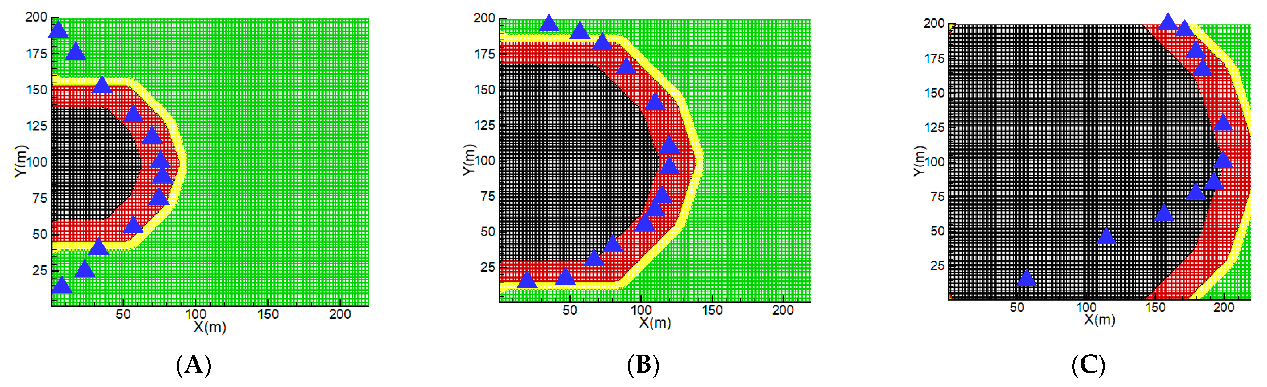
The predicted and observed contours are shown in Figure 3 at times 56 s, 86 s, and 138 s. At 56 s, the flank fire (in the direction perpendicular to the wind) is underestimated by our model, but the head fire (in the wind direction) is in good agreement with the observed fire contour (Figure 3A). At 86 s, the predicted fire contour is in good agreement with the observed fire contour, both for the head fire and the flanking fire (Figure 3B). At 138 s, the change in wind direction caused a shift in the observed fire contour. Due to the lack of information on this change in direction, the average wind direction was used during the simulation. However, the head fire is relatively well predicted (Figure 3C).

4.2. Comparison of Simulations with Empirical Models

The comparison between simulated and experimental results shows whether the simulation provides realistic results. To the best of our knowledge, there are no well-documented experiments on the effectiveness of firebreaks in the savanna zone in Côte d’Ivoire. Therefore, in this section, we use experiments carried out in the Northern Territory of Australia. The operational model derived from these experiments is used. For the success of the comparison, our model should be applied to the same parameters as those considered in the empirical model. To do this, we use the simulation of the F19 experiment presented above, which is one of the experiments used to set up the empirical model [9].

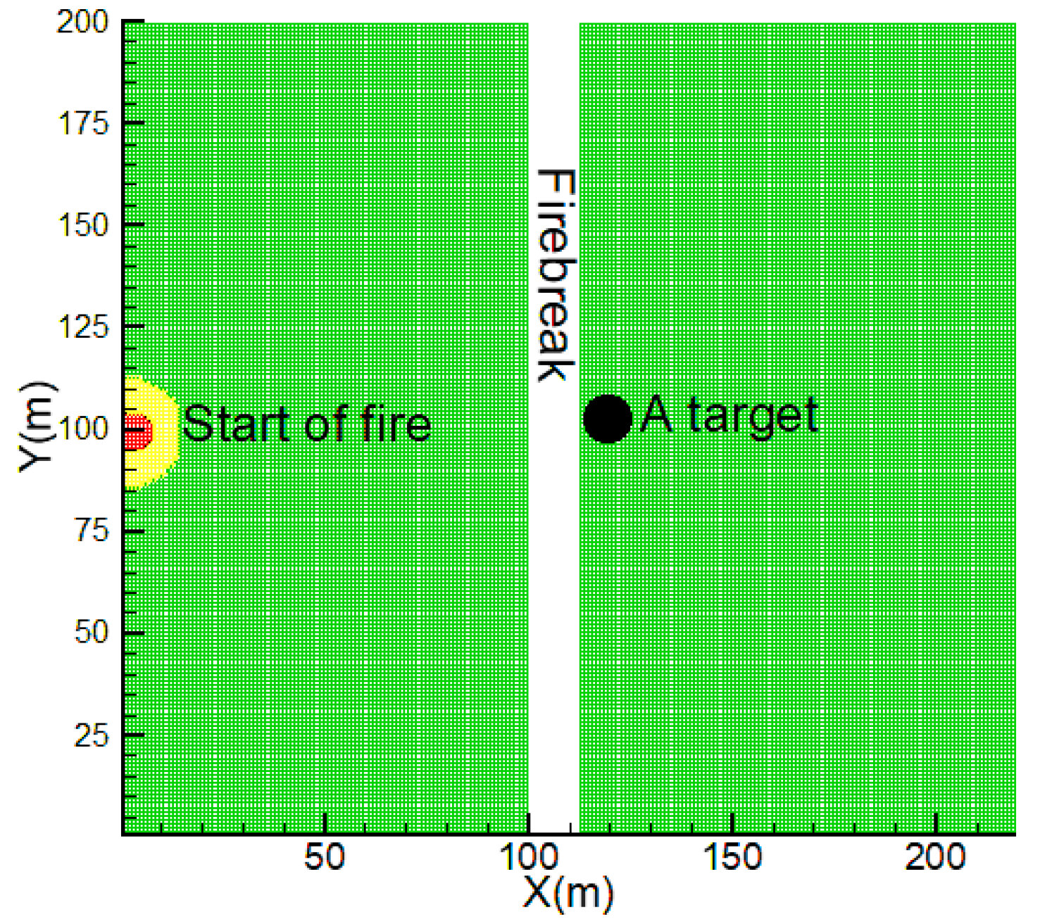
Figure 4 shows the simulation area, the position of the firebreak, and the position of a target. The temperature of the target ($T_t$) as a function of time will be monitored. This temperature will be used to measure the effectiveness of the firebreak in our model. The ignition temperature in our model is 500 K, and the water evaporation temperature is 373 K. If the target temperature is greater than or equal to 500 K ($T_t\ge 500 \mathrm{K}$), this would mean that the fire has broken through the firebreak. If the target temperature is between the water evaporation temperature and the ignition temperature ($373 \mathrm{K}\le T_t<500 \mathrm{K}$), then the target is assumed to be “thermally highly degraded”. When the target temperature is between the ambient temperature ($T_{\infty }$) and the evaporation temperature $T_{\infty }\le T_t<373 \mathrm{K}$, the target is assumed to be “thermally degraded”.

The simulation protocol is presented in

Table 3. Simulation protocol: range of variation of the different parameters. The probability of crossing the firebreak is estimated for each variation.

$\mathbf{Fire}\mathbf{Intensity}\mathit{I}$$\left(\mathsf{M}\mathsf{W}{\mathsf{m}}^{-1}\right)$	$\mathbf{Flame}\mathbf{Length}\mathit{L}\mathit{f}\mathit{l}\left(\mathbf{m}\right)\left(\mathbf{Equation}\right(19\left)\right)$	Width of the Firebreak (m)	Probability of Fire Breaking through the Firebreak (%) (Equation (18))
3	2.35	2	61.3
		4	17.95
		6	2.93
6	3.33	4	39.17
		6	8.16
		8	1.21
9	4.08	6	20.75
		8	3.48
		10	0.49
12	4.71	8	9.62
		10	1.44
		12	0.2
14	5.08	8	17.94
		10	2.93
		12	0.41
16	5.44	8	31
		10	5.84
		12	0.84
18	5.76	8	48
		10	11.3

. The intensity of the fire (and therefore the length of the flame) and the thickness of the firebreak are varied. For each variation, the probability of the fire passing through the firebreak is calculated using Equation (18), and the temperature of the target is recorded during the simulation. The temperature of the target is plotted in Figure 5 against the probability of the fire passing through the firebreak.

It is observed that the temperature of the target is greater than or equal to the ignition temperature for probabilities greater than or equal to 20%, except for one fire. This is the fire with an intensity of $16 {\mathrm{MWm}}^{-1}$ ($Lfl=5.44 \mathrm{m}$) and a firebreak width of 8 m. For probabilities below 20%, the temperature of the target is lower than the ignition temperature. These results indicate that the firebreak was breached by the fire during the simulations for probabilities above 20%. The fire with an intensity of $16 {\mathrm{MWm}}^{-1}$ and a firebreak width of 8 m has a 31% probability of firebreak failure. Although the probability is greater than 20%, the fire did not breach the firebreak. The simulation of this fire is shown in Figure 6. The temperature of the target after 90 s of spread is 415 K.

4.3. Study of the Effectiveness of the Firebreak

To study the effectiveness of the firebreak, we plotted the width of the firebreak against the length of the flame for different ranges of the temperature of the target (see Figure 7). Looking at this figure, it can be seen in general that the temperature of the target is lower than the evaporation temperature of the water when the width of the firebreak is greater than twice the length of the flame. The 8 m thick firebreak was only breached by one fire. A minimum firebreak thickness of twice the flame length would therefore be effective in preventing fire spread.

We tested the effectiveness of this sizing rule on a bushfire in Côte d’Ivoire. We numerically studied the effectiveness of firebreaks by varying some fire parameters. The vegetation characteristics and meteorological data used for the simulations were those of experimental fires carried out in the Lamto reserve in Côte d’Ivoire. These field-scale experiments were used to test the present model [18].

Table 4. Simulation input data.

Variables	Experience Data
Air temperature (K)	308
Ambient wind speed ($\mathrm{m}.{\mathrm{s}}^{-1}$)	4
Dead fuel moisture content (%)	20
Fuel bed height (m)	0.95
Fuel load ($\mathrm{kg}.{\mathrm{m}}^{-2}$)	1.8
Fuel density ($\mathrm{kg}.{\mathrm{m}}^{-3}$)	300
Flame height (m)	3

presents the data used. The combustible vegetation consists of tall grasses with an average height of 0.95 m. This type of vegetation is found in the north and centre of Côte d’Ivoire, where several bushfires are observed every year. Especially during the dry season between December and March. The average fuel load is 1.8 $\mathrm{kg}.{\mathrm{m}}^{-2}$ and the wind speed is 4 m/s. It should be noted that this wind speed is the maximum wind speed observed experimentally.

Figure 8 shows simulations carried out by varying some of the fire parameters. The width of the firebreak is twice the initial length of the flame, i.e., 6 m. Figure 8A shows the firebreak contour with the initial parameters, Figure 8B shows the firebreak contour with a terrain slope of 10%; in Figure 8C,D, the wind speed is doubled (i.e., $8{\mathrm{ms}}^{-1}$). In general, the increase in wind speed leads to an increase in the length of the flame. This is because as the wind speed increases, the amount of oxygen required for combustion also increases. Therefore, in Figure 8C the flame length is increased by 1 m and in Figure 8D by 2 m.

The fire did not breach the firebreak despite the slope (Figure 8B), but the fuel on the other side of the firebreak is more degraded than in the case without slope (Figure 8A). The firebreak remains effective when the wind speed is doubled, and the flame length is increased by 1 m (Figure 8C). However, when the length of the flame is increased by 2 m, the fire crosses through the firebreak.

4.4. Discussion

When the probability of crossing the firebreak calculated by the empirical model of Wilson (1988) is higher than 20%, the fire crosses the firebreak in our model. On the other hand, when the probability of crossing the firebreak is strictly less than 20%, the firebreak is not crossed, but the fuel on the other side of the firebreak is more or less degraded, depending on the case. This comparison proves that our simulation results are realistic.

In the simulations, firebreaks with a width approximately equal to the length of the flame were easily breached by the fire. When the width of the firebreak was slightly less than twice the length of the flame, the fire did not breach the firewall but thermally degraded the fuel on the other side of the firebreak. Most firebreaks with a width of about twice the flame length were not breached by the fire. The probability of the firebreak being breached in these cases was generally less than 20%, as estimated by the empirical model of Wilson (1988). The effectiveness of the firebreak is therefore closely related to the length of the flame. The design rule of taking twice the flame length as the firebreak width is effective even in the presence of a slope. However, when the wind speed increases, the firebreak is effective under certain conditions. These conditions are related to the length of the flame. The firebreak design rule based on flame length is also used by Butler and Cohen [10]. The problem with this design rule is the choice of the relevant flame length to be used as the basis for the calculation.

It was also found that firebreaks with a minimum width of 8 m were effective for most flame lengths. However, for the 5.76 m flame length, the 8 m wide firebreak was breached by the fire. Flame lengths in our savannas rarely reach 5 m. This is evidenced by savanna fire experiments [18,22]. The minimum width of 8 m is therefore appropriate for an effective firebreak against bushfire spread in Côte d’Ivoire. These results are in agreement with those obtained by Frost et al. (2022) [23], who recommend a minimum width of 8 m for a grass fire.

The means to fight forest fires are expensive and not within reach of all African countries. For these countries, prevention is paramount, including close monitoring of risk areas, prescribed burning, and firebreaks.

This study has shown that fire behaviour models can help in rational decision-making to prevent bushfires. They can help to establish rules for the design and maintenance of firebreaks in a sufficiently objective manner [24]. Models and modelling are an integral part of modern fire management practices [23,25].

5. Conclusions

We studied the effectiveness of a firebreak in a savanna area using a 2D fire spread model. The ability of the model to perform this study was tested by an empirical model based on savanna fire experiments. A good agreement was found between the results.

The simulations showed that a firebreak width equal to twice the flame length was effective in preventing the progression of a savanna fire. This design rule remains difficult because it depends on a fire-related parameter. However, the study showed that a firebreak with a minimum width of 8 m was effective in stopping a bushfire. The presence of trees in the vicinity of the firebreak was not taken into account in this study.

This study is part of a series whose objective is to develop an operational simulation tool for use by vegetation firefighting services in Côte d’Ivoire.