
Using Geographic Information to Analyze Wildland Firefighter Situational Awareness: Impacts of Spatial Resolution on Visibility Assessment


Abstract
:1. Introduction
- Introduce an approach for quantifying visibility at the scale of wildland firefighter handlines.
- Determine the effect of spatial resolution of lidar-derived elevation data on calculated visibility in a forested environment and evaluate implications for wildland firefighter safety assessment.
- Use geospatial information to assess the general safety and situational awareness of handlines based on landscape metrics and visibility.
2. Background
3. Materials and Methods
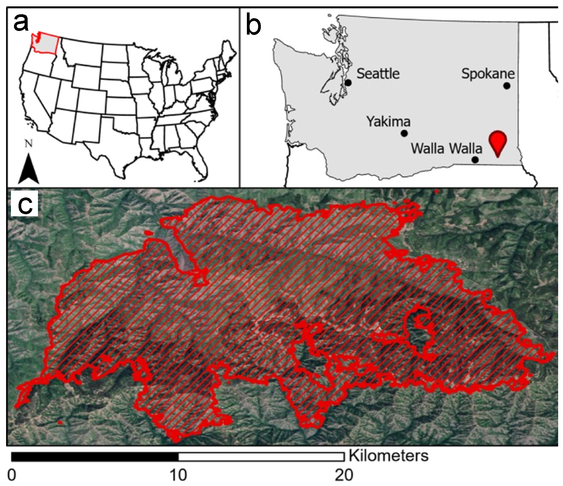
3.1. Study Area
3.2. Data
3.2.1. Digital Elevation Models
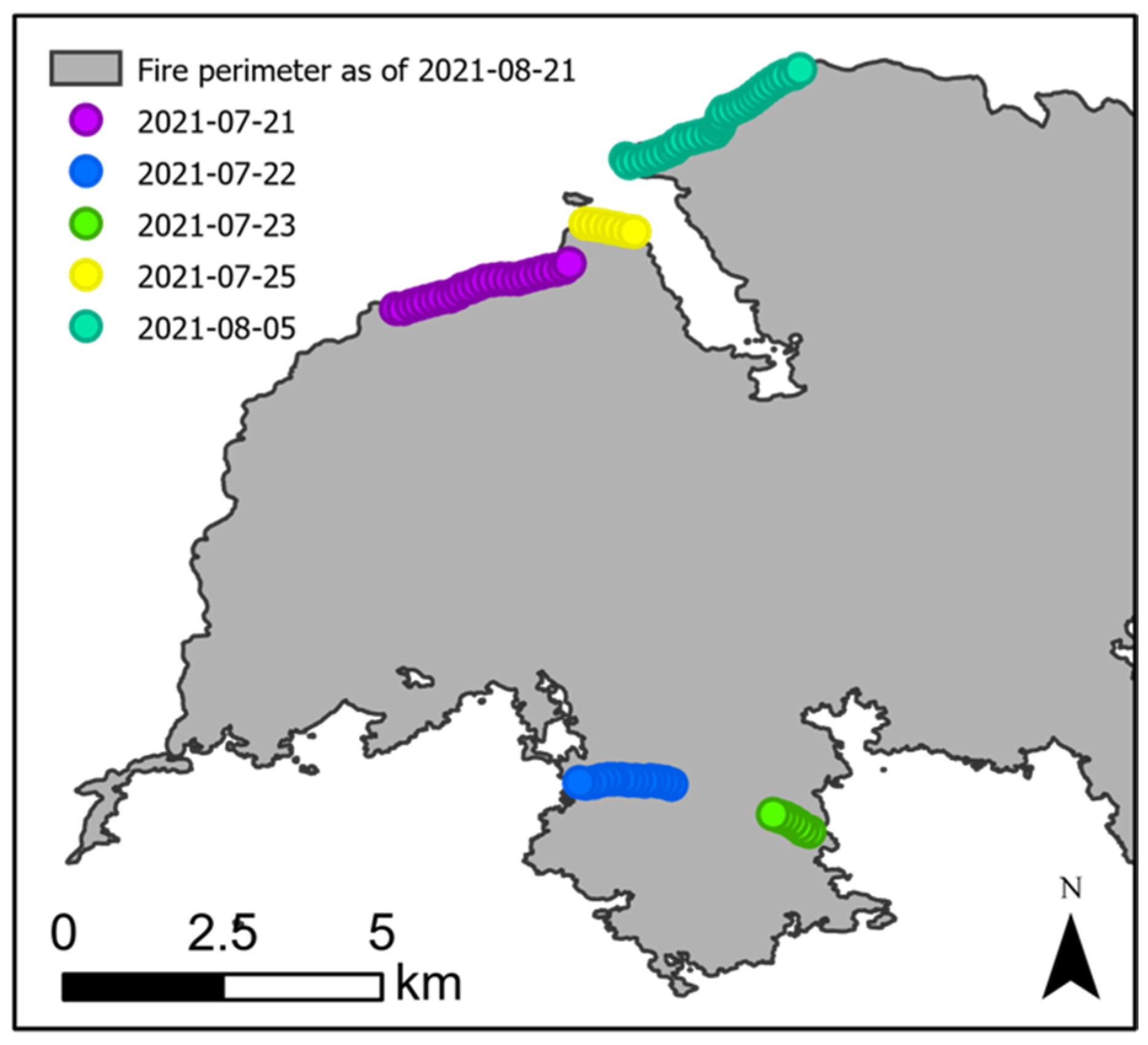
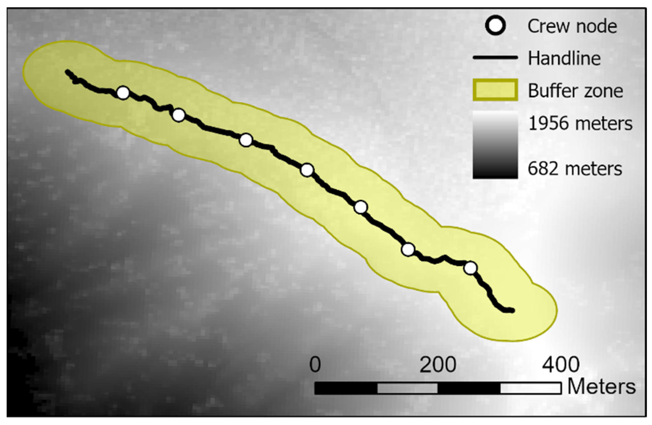
3.2.2. Handlines
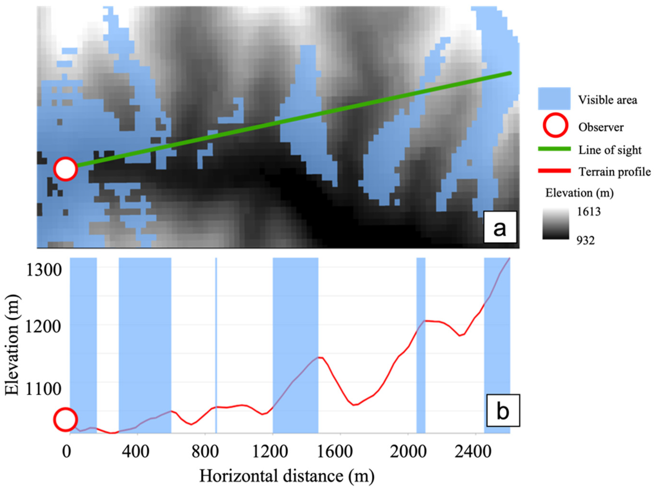
3.3. Viewshed Processing
3.4. Handline Landscape Metrics
4. Results
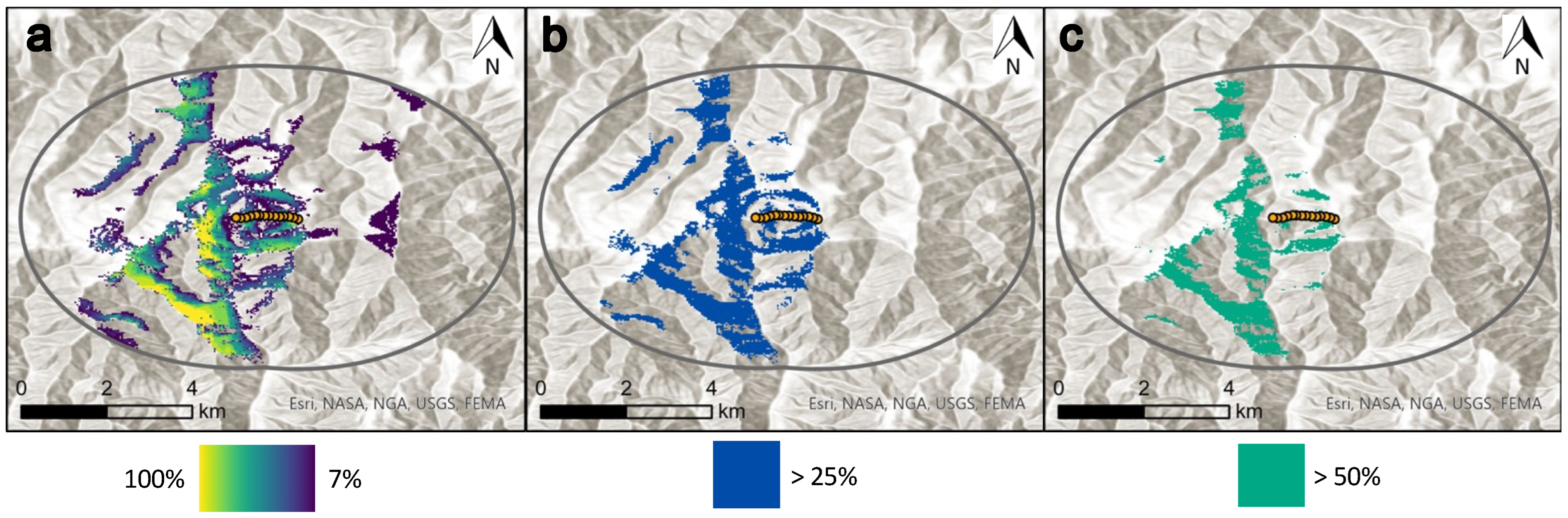
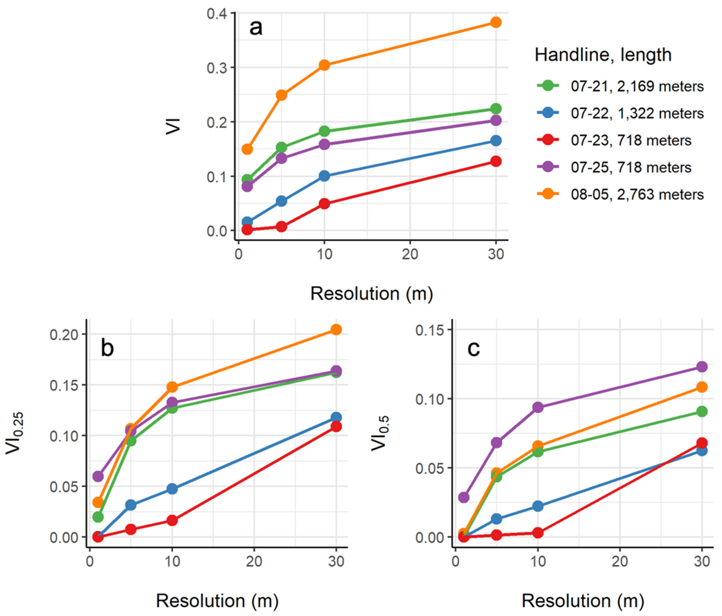
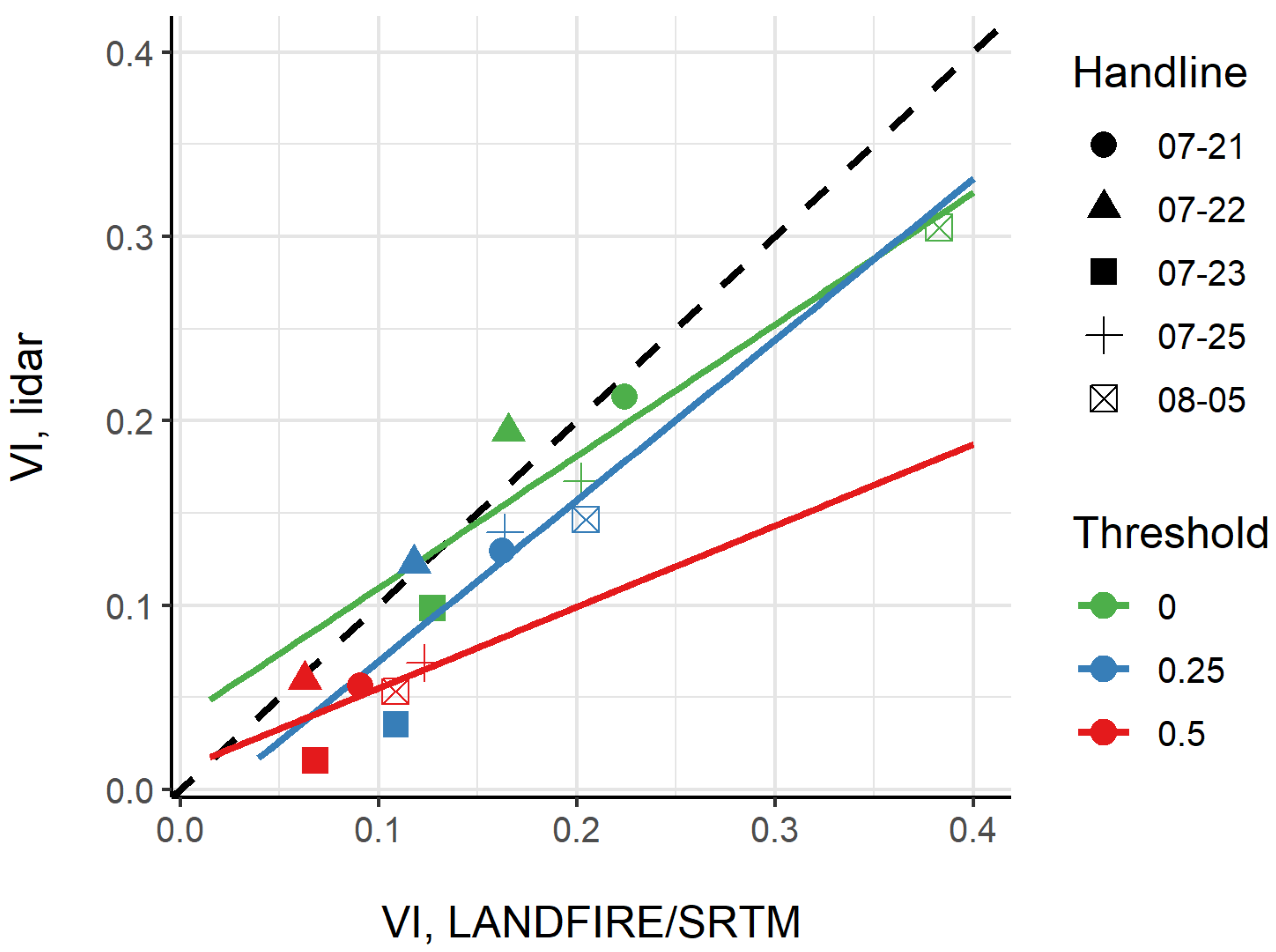
4.1. Effect of Spatial Resolution of Elevation Data on Calculated Visibility
4.2. Handline Landscape Metrics
5. Discussion
6. Conclusions
- Estimating visibility at the handline level through viewshed analysis can assist wildland firefighters with evaluating potential limitations to situational awareness
- Spatial resolution has a pronounced effect on the estimation of visibility and therefore must be taken into consideration prior to use in fire management operations
- Coarser resolution DSMs (≥10 m), including those created from lidar data and from more widely available LANDFIRE and SRTM products, likely overestimate visibility
- Viewshed analysis conducted at a spatial resolution of 5 m provides a high degree of landscape structural detail while significantly reducing processing time and storage requirements as compared to the same analysis conducted at finer resolutions (1 m)
- Canopy cover and slope displayed strong linear relationships with visibility
- Landscape metrics, when presented in conjunction with visibility analyses, offer the potential to improve situational awareness and/or inform management decisions
Author Contributions
Funding
Institutional Review Board Statement
Informed Consent Statement
Acknowledgments
Conflicts of Interest
Abbreviations
| Acronym | Significance |
| CH | Canopy height |
| CHM | Canopy height model |
| DEM | Digital elevation model |
| DSM | Digital surface model |
| DTM | Digital terrain model |
| EVH | Existing Vegetation Height |
| LCES | Lookouts, Communications, Escape Routes, Safety Zones |
| NWCG | National Wildfire Coordinating Group |
| SRTM | Shuttle Radar Topography Mission |
| TPI | Topographic Position Index |
| VI | Visibility Index |
References
- Page, W.G.; Freeborn, P.H.; Butler, B.W.; Jolly, W.M. A Review of US Wildland Firefighter Entrapments: Trends, Important Environmental Factors and Research Needs. Int. J. Wildland Fire 2019, 28, 551. [Google Scholar] [CrossRef]
- National Wildfire Coordinating Group. NWCG Report on Wildland Firefighter Fatalities in the United States: 2007–2016. 2017. Available online: https://www.nwcg.gov/sites/default/files/publications/pms841.pdf (accessed on 6 September 2022).
- Arizona State Forestry Division. Yarnell Hill Serious Accident Investigation Report. 2013. Available online: https://wildfiretoday.com/documents/Yarnell_Hill_Fire_report.pdf (accessed on 15 September 2022).
- Abatzoglou, J.T.; Battisti, D.S.; Williams, A.P.; Hansen, W.D.; Harvey, B.J.; Kolden, C.A. Projected Increases in Western US Forest Fire despite Growing Fuel Constraints. Commun. Earth Environ. 2021, 2, 227. [Google Scholar] [CrossRef]
- Balch, J.K.; Schoennagel, T.; Williams, A.P.; Abatzoglou, J.T.; Cattau, M.E.; Mietkiewicz, N.P.; Denis, L.A.S. Switching on the Big Burn of 2017. Fire 2018, 1, 17. [Google Scholar] [CrossRef]
- Dennison, P.E.; Brewer, S.C.; Arnold, J.D.; Moritz, M.A. Large Wildfire Trends in the Western United States, 1984–2011. Geophys. Res. Lett. 2014, 41, 2928–2933. [Google Scholar] [CrossRef]
- Gleason, P. Lookouts, Communication, Escape Routes and Safety Zones, “LCES”. 1991. Available online: https://www.nwcg.gov/sites/default/files/wfldp/docs/lces-gleason.pdf (accessed on 28 September 2022).
- NWCG Glossary of Wildland Fire. Available online: https://www.nwcg.gov/glossary/a-z (accessed on 6 September 2022).
- California Conversvation Corps. 10 Standard Orders & 18 Watch Outs. 2019. Available online: https://ccc.ca.gov/wp-content/uploads/2019/08/CCC-10-Standard-Orders-18-Watch-Outs.pdf (accessed on 6 September 2022).
- Baek, H.; Lim, J. Design of Future UAV-Relay Tactical Data Link for Reliable UAV Control and Situational Awareness. IEEE Commun. Mag. 2018, 56, 144–150. [Google Scholar] [CrossRef]
- Nofi, A. Defining and Measuring Shared Situational Awareness; Center for Naval Analyses: Alexandria, VA, USA, 2000. [Google Scholar]
- Gillespie, B.M.; Gwinner, K.; Fairweather, N.; Chaboyer, W. Building Shared Situational Awareness in Surgery through Distributed Dialog. J. Multidiscip Healthc 2013, 6, 109–118. [Google Scholar] [CrossRef] [PubMed]
- Graafland, M.; Schraagen, J.M.C.; Boermeester, M.A.; Bemelman, W.A.; Schijven, M.P. Training Situational Awareness to Reduce Surgical Errors in the Operating Room. Br. J. Surg. 2014, 102, 16–23. [Google Scholar] [CrossRef] [PubMed]
- Jolly, W.M.; Freeborn, P.H. Towards Improving Wildland Firefighter Situational Awareness through Daily Fire Behaviour Risk Assessments in the US Northern Rockies and Northern Great Basin. Int. J. Wildland Fire 2017, 26, 574. [Google Scholar] [CrossRef]
- Page, W.G.; Butler, B.W. Fuel and Topographic Influences on Wildland Firefighter Burnover Fatalities in Southern California. Int. J. Wildland Fire 2018, 27, 141. [Google Scholar] [CrossRef]
- Stanton, N.A.; Chambers, P.R.G.; Piggott, J. Situational Awareness and Safety. Saf. Sci. 2001, 39, 189–204. [Google Scholar] [CrossRef] [Green Version]
- Mangan, R. Investigating Wildland Fire Entrapments; United States Department of Agriculture: Missoula, MT, USA, 1995. [Google Scholar]
- Lahaye, S.; Sharples, J.; Matthews, S.; Heemstra, S.; Price, O.; Badlan, R. How Do Weather and Terrain Contribute to Firefighter Entrapments in Australia? Int. J. Wildland Fire 2018, 27, 85. [Google Scholar] [CrossRef]
- Page, W.G.; Freeborn, P.H.; Butler, B.W.; Jolly, W.M. A Classification of US Wildland Firefighter Entrapments Based on Coincident Fuels, Weather, and Topography. Fire 2019, 2, 52. [Google Scholar] [CrossRef]
- Campbell, M.J.; Page, W.G.; Dennison, P.E.; Butler, B.W. Escape Route Index: A Spatially-Explicit Measure of Wildland Firefighter Egress Capacity. Fire 2019, 2, 40. [Google Scholar] [CrossRef]
- Campbell, M.J.; Dennison, P.E.; Butler, B.W.; Page, W.G. Using Crowdsourced Fitness Tracker Data to Model the Relationship between Slope and Travel Rates. Appl. Geogr. 2019, 106, 93–107. [Google Scholar] [CrossRef]
- Campbell, M.J.; Dennison, P.E.; Butler, B.W. A LiDAR-Based Analysis of the Effects of Slope, Vegetation Density, and Ground Surface Roughness on Travel Rates for Wildland Firefighter Escape Route Mapping. Int. J. Wildland Fire 2017, 26, 884. [Google Scholar] [CrossRef]
- Sullivan, P.R.; Campbell, M.J.; Dennison, P.E.; Brewer, S.C.; Butler, B.W. Modeling Wildland Firefighter Travel Rates by Terrain Slope: Results from GPS-Tracking of Type 1 Crew Movement. Fire 2020, 3, 52. [Google Scholar] [CrossRef]
- Campbell, M.J.; Dennison, P.E.; Thompson, M.P.; Butler, B.W. Assessing Potential Safety Zone Suitability Using a New Online Mapping Tool. Fire 2022, 5, 5. [Google Scholar] [CrossRef]
- Campbell, M.J.; Dennison, P.E.; Butler, B.W. Safe Separation Distance Score: A New Metric for Evaluating Wildland Firefighter Safety Zones Using Lidar. Int. J. Geogr. Inf. Sci. 2017, 31, 1448–1466. [Google Scholar] [CrossRef]
- Dennison, P.E.; Fryer, G.K.; Cova, T.J. Identification of Firefighter Safety Zones Using Lidar. Environ. Model. Softw. 2014, 59, 91–97. [Google Scholar] [CrossRef]
- National Wildfire Coordinating Group. S-130 Unit 9: Handline Techniques. In NWCG Instructor Guide; pp. 1–22. Available online: https://training.nwcg.gov/dl/s130/s-130-ig09.pdf (accessed on 15 September 2022).
- O’Connor, C.D.; Calkin, D.E.; Thompson, M.P. An Empirical Machine Learning Method for Predicting Potential Fire Control Locations for Pre-Fire Planning and Operational Fire Management. Int. J. Wildland Fire 2017, 26, 587. [Google Scholar] [CrossRef]
- Rodríguez y Silva, F.; O’Connor, C.D.; Thompson, M.P.; Molina Martínez, J.R.; Calkin, D.E. Modelling Suppression Difficulty: Current and Future Applications. Int. J. Wildland Fire 2020, 29, 739. [Google Scholar] [CrossRef]
- National Interagency Fire Center. Chapter 7: Safety and Risk Management. In Interagency Standards for Fire and Fire Aviation Operations; 2022. Available online: https://www.nifc.gov/sites/default/files/redbook-files/Chapter07.pdf (accessed on 15 September 2022).
- Lefsky, M.A.; Cohen, W.B.; Parker, G.G.; Harding, D.J. Lidar Remote Sensing for Ecosystem Studies. BioScience 2002, 52, 19. [Google Scholar] [CrossRef]
- Gallant, J.C.; Wilson, J.P. Primary Topographic Attributes. In Terrain Analysis: Principles and Applications; John Wiley & Sons Inc.: Hoboken, NJ, USA, 2000; Volume 7, pp. 51–85. ISBN 0-471-32188-5. [Google Scholar]
- Weiss, A. Topographic Position and Landforms Analysis. In Proceedings of the ESRI Users Conference, San Diego, CA, USA, 12 July 2001. [Google Scholar]
- Evans, J.S.; Hudak, A.T. A Multiscale Curvature Algorithm for Classifying Discrete Return LiDAR in Forested Environments. IEEE Trans. Geosci. Remote Sens. 2007, 45, 1029–1038. [Google Scholar] [CrossRef]
- Meng, X.; Currit, N.; Zhao, K. Ground Filtering Algorithms for Airborne LiDAR Data: A Review of Critical Issues. Remote Sens. 2010, 2, 833–860. [Google Scholar] [CrossRef]
- Murgoitio, J.J.; Shrestha, R.; Glenn, N.F.; Spaete, L.P. Improved Visibility Calculations with Tree Trunk Obstruction Modeling from Aerial LiDAR. Int. J. Geogr. Inf. Sci. 2013, 27, 1865–1883. [Google Scholar] [CrossRef]
- Vukomanovic, J.; Singh, K.K.; Petrasova, A.; Vogler, J.B. Not Seeing the Forest for the Trees: Modeling Exurban Viewscapes with LiDAR. Landsc. Urban Plan. 2018, 170, 169–176. [Google Scholar] [CrossRef]
- Bartie, P.; Reitsma, F.; Kingham, S.; Mills, S. Incorporating Vegetation into Visual Exposure Modelling in Urban Environments. Int. J. Geogr. Inf. Sci. 2011, 25, 851–868. [Google Scholar] [CrossRef]
- Yu, S.; Yu, B.; Song, W.; Wu, B.; Zhou, J.; Huang, Y.; Wu, J.; Zhao, F.; Mao, W. View-Based Greenery: A Three-Dimensional Assessment of City Buildings’ Green Visibility Using Floor Green View Index. Landsc. Urban Plan. 2016, 152, 13–26. [Google Scholar] [CrossRef]
- Chamberlain, B.C.; Meitner, M.J. A Route-Based Visibility Analysis for Landscape Management. Landsc. Urban Plan. 2013, 111, 13–24. [Google Scholar] [CrossRef]
- Fisher, P.; Farrelly, C.; Maddocks, A.; Ruggles, C. Spatial Analysis of Visible Areas from the Bronze Age Cairns of Mull. J. Archaeol. Sci. 1997, 24, 581–592. [Google Scholar] [CrossRef]
- Green Ridge Fire. Available online: https://inciweb.nwcg.gov/incident/7628/ (accessed on 6 September 2022).
- Sugarbaker, L.; Constance, E.W.; Heidemann, H.K.; Jason, A.L.; Saghy, D.L.; Stoker, J.M. The 3D Elevation Program Initiative—A Call for Action; USGS: Reston, VA, USA, 2014. [Google Scholar]
- Topographic Data Quality Levels (QLs). Available online: www.usgs.gov/3d-elevation-program/topographic-data-quality-levels-qls (accessed on 6 September 2022).
- Isenburg, M. LAStools; Rapidlasso GmbH: Gilching, Germany, 2015. [Google Scholar]
- Farr, T.G.; Kobrick, M. Shuttle Radar Topography Mission Produces a Wealth of Data. Eos Trans. Am. Geophys. Union 2000, 81, 583–585. [Google Scholar] [CrossRef]
- ESRI. How Geodesic Viewshed Works. Available online: https://pro.arcgis.com/en/pro-app/2.8/tool-reference/spatial-analyst/how-viewshed-2-works.htm (accessed on 6 September 2022).
- Franklin, W.R.; Ray, C.K. Higher Isn’t Necessarily Better: Visibility Algorithms and Experiments. Adv. GIS Res. 1994, 2, 22. [Google Scholar]
- Campbell, M.J.; Dennison, P.E.; Hudak, A.T.; Parham, L.M.; Butler, B.W. Quantifying Understory Vegetation Density Using Small-Footprint Airborne Lidar. Remote Sens. Environ. 2018, 215, 330–342. [Google Scholar] [CrossRef]
- Existing Vegetation Height, LF 2016 Remap [LF 2.0.0]. Available online: https://landfire.gov/evh.php (accessed on 6 September 2022).
- Data Access: Fire Level Geospatial Data. Available online: https://mtbs.gov/direct-download (accessed on 6 September 2022).
- Orange County California Fire Authority Informational Summary Report of Serious or Near Serious Injuries, Illnesses and Accidents—Firefighter Burn Over October 26, 2020 Silverado Incident. 2020. Available online: https://wildfiretoday.com/documents/Green-Sheet-OCFA-Final-_1_.pdf (accessed on 15 September 2022).
- USDA Forest Service, Pacific Southwest Region, Shasta-Trinity National Forest. Is That the Freight Train I’m Hearing? McFarland Fire Entrapment FLA. 2021. Available online: https://www.wildfirelessons.net/HigherLogic/System/DownloadDocumentFile.ashx?DocumentFileKey=64ec35f7-9ee7-48f5-a821-be3d9f6a3738&forceDialog=0 (accessed on 15 September 2022).


| Handline | Number of Crew Nodes | Fire Growth 1 (Hectares) | Total Fire Area 1 (Hectares) |
|---|---|---|---|
| 2021-07-21 | 24 | 679 | 1313 |
| 2021-07-22 | 14 | 270 | 1583 |
| 2021-07-23 | 7 | 271 | 1853 |
| 2021-07-25 | 7 | 270 | 2381 |
| 2021-08-05 | 30 | 501 | 5458 |
| Landscape Metric | Definition | Derived from |
|---|---|---|
| Slope | The gradient or steepness of a surface | DTM |
| Canopy height (CH) | Height of vegetation across a landscape | CHM |
| Canopy cover | Proportion of the landscape covered by vegetation of a certain height | CHM |
| Topographic position index (TPI) | Relative elevation, relies on the elevation of a central pixel and the average elevation of a surrounding annulus with predefined inner and outer radii [32,33] | DTM |
| Threshold | Slope | y-Intercept | R2 | p-Value |
|---|---|---|---|---|
| 0 | 0.72 | 3.79 | 0.87 | 0.02 |
| 0.25 | 0.87 | −1.74 | 0.56 | 0.15 |
| 0.5 | 0.44 | 1.08 | 0.31 | 0.33 |
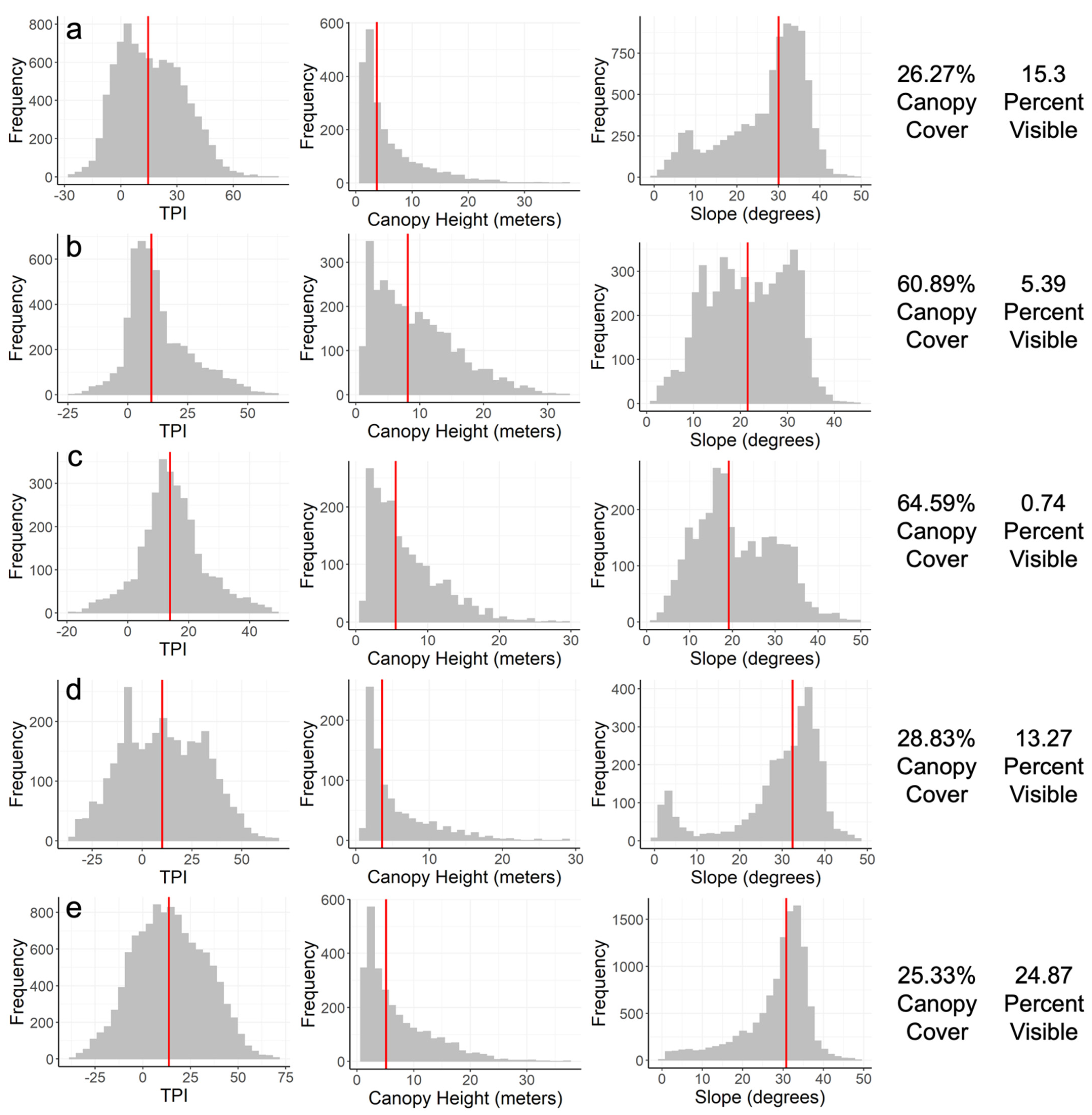
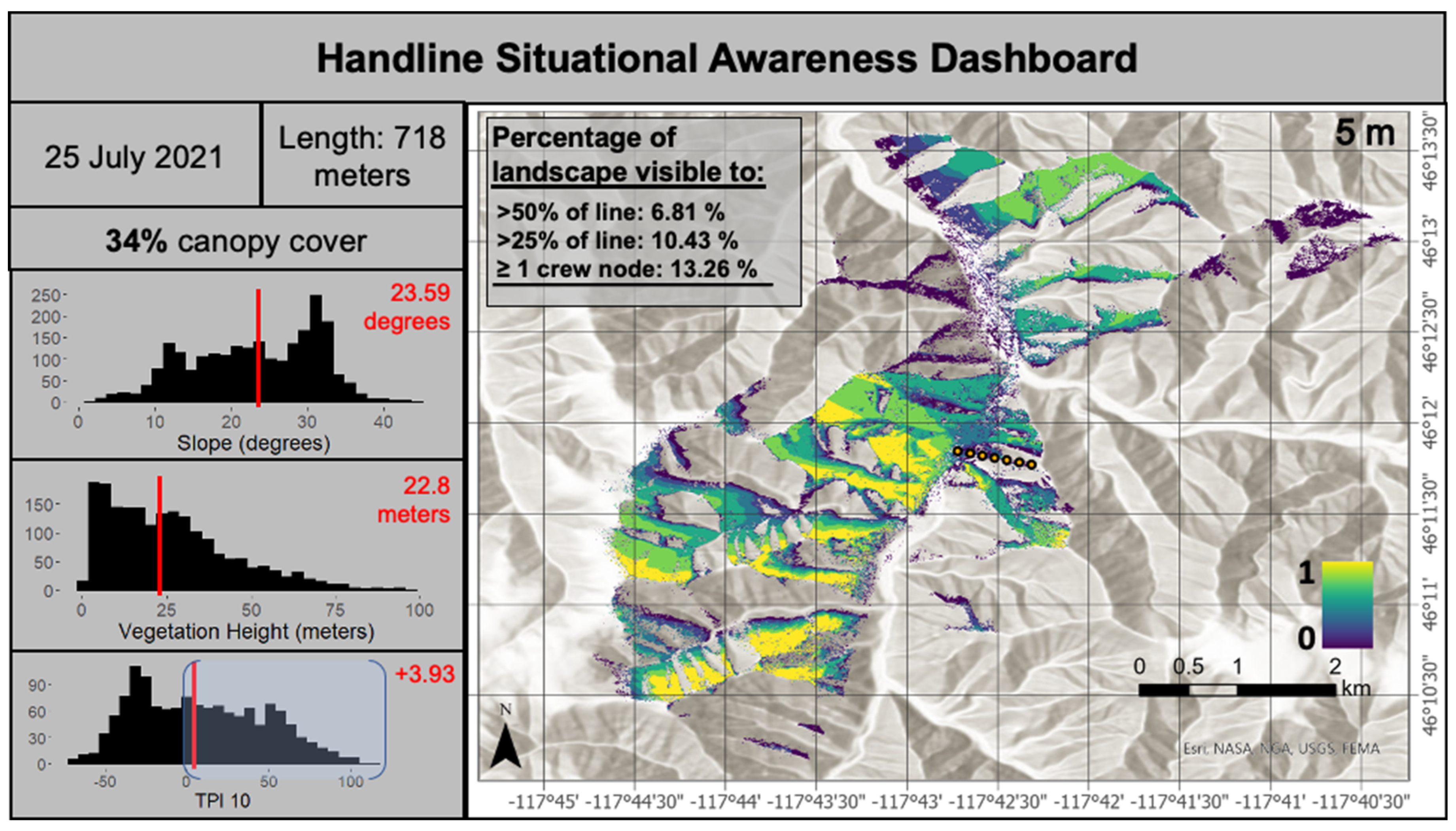
| Handline | Length (m) | Canopy Cover (%) | Median Canopy Height (m) | Median Slope (Degrees) | Median TPI | VI 1 |
|---|---|---|---|---|---|---|
| 2021-07-21 | 2169 | 26.27 | 3.69 | 30.07 | 14.62 | 0.153 |
| 2021-07-22 | 1322 | 60.89 | 8.14 | 21.54 | 9.83 | 0.054 |
| 2021-07-23 | 718 | 64.59 | 5.56 | 19.16 | 13.91 | 0.007 |
| 2021-07-25 | 718 | 28.83 | 3.57 | 32.43 | 10.01 | 0.133 |
| 2021-08-05 | 2763 | 25.33 | 5.16 | 30.79 | 13.71 | 0.249 |
Publisher’s Note: MDPI stays neutral with regard to jurisdictional claims in published maps and institutional affiliations. |
© 2022 by the authors. Licensee MDPI, Basel, Switzerland. This article is an open access article distributed under the terms and conditions of the Creative Commons Attribution (CC BY) license (https://creativecommons.org/licenses/by/4.0/).
Share and Cite
Mistick, K.A.; Dennison, P.E.; Campbell, M.J.; Thompson, M.P. Using Geographic Information to Analyze Wildland Firefighter Situational Awareness: Impacts of Spatial Resolution on Visibility Assessment. Fire 2022, 5, 151. https://doi.org/10.3390/fire5050151
Mistick KA, Dennison PE, Campbell MJ, Thompson MP. Using Geographic Information to Analyze Wildland Firefighter Situational Awareness: Impacts of Spatial Resolution on Visibility Assessment. Fire. 2022; 5(5):151. https://doi.org/10.3390/fire5050151
Chicago/Turabian StyleMistick, Katherine A., Philip E. Dennison, Michael J. Campbell, and Matthew P. Thompson. 2022. "Using Geographic Information to Analyze Wildland Firefighter Situational Awareness: Impacts of Spatial Resolution on Visibility Assessment" Fire 5, no. 5: 151. https://doi.org/10.3390/fire5050151
APA StyleMistick, K. A., Dennison, P. E., Campbell, M. J., & Thompson, M. P. (2022). Using Geographic Information to Analyze Wildland Firefighter Situational Awareness: Impacts of Spatial Resolution on Visibility Assessment. Fire, 5(5), 151. https://doi.org/10.3390/fire5050151