Evaluating Satellite Fire Detection Products and an Ensemble Approach for Estimating Burned Area in the United States

Abstract

Fire location and burning area are essential parameters for estimating fire emissions. However, ground-based fire data (such as fire perimeters from incident reports) are often not available with the timeliness required for real-time forecasting. Fire detection products derived from satellite instruments such as the GOES-16 Advanced Baseline Imager or MODIS, on the other hand, are available in near real-time. Using a ground fire dataset of 2699 fires during 2017–2019, we fit a series of linear models that use multiple satellite fire detection products (HMS aggregate fire product, GOES-16, MODIS, and VIIRS) to assess the ability of satellite data to detect and estimate total burned area. It was found that on average models fit with fire detections from GOES-16 products performed better than those developed from other satellites in the study (modelled R² = 0.84 and predictive R² = 0.88). However, no single satellite product was found to best estimate incident burned area, highlighting the need for an ensemble approach. With our proposed modelling ensemble, we demonstrate its ability to estimate burned area and suggest its further use in daily fire tracking and emissions-modeling frameworks.

1. Introduction

Wildland fires release large amounts of aerosols and trace gases into the atmosphere, which has short- and long-term impacts on air quality [1], public health [2] and the global carbon cycle [3,4]. The location and amount of area burning are primary inputs to algorithms that quantify the aerosols and trace gases emitted, and accurately determining these inputs is critical. Ground tracking of actively burning area or even fire location is not uniform across land ownerships and regions. Where available, access is often not quick enough for near real-time air quality forecasting. Alternatively, satellites provide consistent fire detection products that cover large areas and are readily available in near real-time. Because of this, many studies that focus on estimating biomass burning emissions on regional and global scales use satellite fire detection data [5,6,7,8,9,10,11,12,13,14,15]. Use of satellite data for this purpose requires care as differing spatial resolutions, sensor type, and measurement timings result in detection capabilities that vary by satellite and fire detection package.

The Visible Infrared Imaging Radiometer Suite (VIIRS) packages aboard the Suomi NPP and NOAA-20 satellites can generally detect smaller, cooler fires than can the Geostationary Operational Environmental Satellite (GOES) due to their higher spatial resolution (375 m when overhead) [16,17]. On the other hand, because VIIRS platforms are polar orbiting, at mid-latitudes they will provide only 3–4 looks per day and are not likely to be directly over a given fire during its maximum activity. The GOES-16 and -17 geostationary satellites can provide continual images or fire pixels at 5-min intervals, 1-min in some cases, and can capture fires that burned quickly or are obstructed by clouds or heavy smoke, provided there are breaks at some point during the day. However, GOES’s nominal 2 km resolution stretches away from nadir and at mid-latitudes is relatively coarse. The MODerate Resolution Imaging Spectroradiometer (MODIS) instrument aboard two polar orbiting satellites, Aqua and Terra, provide 2 looks per day at a moderate 1 km resolution.

The ability of satellites to detect fire is also heavily influenced by the type of vegetation that is burning [18,19]. For example, quick burning fuels, such as grasslands, can cause even large fires to burnout quickly, and thus be potentially missed by polar orbiting satellites. Polar systems work best when breaks in cloud and heavy smoke and rapid fire growth occur during their specific overflights times. Fires in vegetation like conifer forest, on the other hand, often have longer durations with correspondingly longer detection windows. Vegetation also puts constraints on the amount of biomass that can burn, which directly effects the amount of energy released from a fire (i.e., fire intensity) and how visible that energy is to satellites. Conversely, vegetation with large canopy cover can obscure lower intensity burns when the flames are below canopy level. The result is regionalized differences in fire detection capabilities based largely on the typical local vegetation cover and fuel moistures that determine typical fire behavior in that region [20].

Determining area burning from fire detections requires the further step of assigning each hotspot or collection of hotspots an area estimate. Assigning areas based on the overall satellite sensor’s pixel spatial coverage overestimates the actual burning area, as satellite sensors often detect subpixel fires, so statistical relationships are needed that create best fit estimates of burning area [21,22,23,24]. These need to account for regional and vegetation detection differences as well as the differences between the various sensors and systems.

In this study, we describe a novel statistical method using fire detection hotspot counts to improve estimates of burning area across the contiguous United States. This method takes advantage of multiple satellite fire detection products to compensate for limitations that can arise from using a single satellite product. The model is specifically designed with near real-time daily estimation as well as ease of utility in mind to meet the needs of decision support systems, such as fire emissions models and smoke forecasts that require rapidly updated information [7]. The goals are to both do retrospective assessments of overall cumulative burned area and to best quantify and track daily active burning.

2. Materials and Methods

This work follows three parts. First, satellite fire detection data from specific satellites, as well as an aggregate system, are analyzed against ground reported data to find statistical fits specific to ecosystem type that can estimate a fire’s cumulative burned area. These are assessed to determine which satellite products appear to allow for the best estimates. Next, we examine the ability of the derived statistical models to track individual fire growth. Finally, we examine whether the use of multiple satellite models, through an ensemble approach, can perform better at these tasks.

2.1. Data

In this study we utilize satellite fire hotspot products and a ground-based fire perimeter dataset across CONUS and Alaska for the period 2017–2020. Data from 2017–2019 were used as training data, and data from 2020 were used as a model validation set.

2.1.1. Satellite Fire Detection Data

Satellite fire detection products were obtained directly from their sources: GOES-16 Advanced Baseline Imager (ABI) Level 2 Fire Detection/Hot Spot Characterization (FDC), MODIS thermal anomalies from both Aqua and Terra satellites, and two VIIRS packages at varying resolutions (

Table 1. Satellite fire detection data used in this study.

Satellite	Instrument	Product	Study Name	Spatial Resolution (at Nadir)	Temporal Resolution
GOES-16	ABI	FDC * [25,26]	GOES-16	2 km	5-min
Terra	MODIS	MCD14ML * [27]	MODIS Terra	1 km	Daily
Aqua	MODIS	MCD14ML [27]	MODIS Aqua	1 km	Daily
Suomi	VIIRS	VNP14v001 [28]	SNPP VIIRS 750 m	750 m	Daily
Suomi	VIIRS	VNP14IMG * [29]	SNPP VIIRS 375 m	375 m	Daily
GOES-16	ABI	HMS [30]	HMS GOES-16	2 km	5-min
Terra	MODIS	HMS [30]	HMS MODIS Terra	1 km	Daily
Suomi	VIIRS	HMS [30]	HMS SNPP VIIRS	375 m	Daily
NOAA 20	VIIRS	HMS [30]	HMS NOAA 20 VIIRS	375 m	Daily

* Source also available through the NOAA Hazard Mapping System (HMS).

). Data from the MODIS instrument were further separated by satellite, Aqua or Terra, for model fitting due to different overpass timings which could affect detection or model fit. Additionally, data for several of these satellites were also obtained through the U.S. National Oceanic and Atmospheric Administration (NOAA) Hazard Mapping System (HMS) data feed.

Fire detections included in HMS are quality controlled by expert image analysts to remove false detections and locations associated with persistent sources and urban environment, and to add detections after referring to satellite imagery. For this reason, this data can differ from the originally sourced data. We choose to include both the originally sourced data and the HMS version, where available, as separate sources for analysis (Note: NOAA 20 VIIRS data were only available from the HMS source for this study). To distinguish, we prefix HMS sourced data with “HMS” as in HMS GOES-16, whereas GOES-16 alone refer to the originally sourced GOES-16 data product. The HMS obtained data closely matched the results of the originally sourced data, however, we elected to keep both as they proved to function differently for individual fire tracking and modelling results.

2.1.2. Ground-Based Fire Incident Data

Ground-based fire data are obtained from the Geospatial Multi-Agency Coordination (GeoMAC; https://data-nifc.opendata.arcgis.com; accessed on 3 May 2020) dataset (2017–2019) and National Interagency Fire Center (NIFC; https://data-nifc.opendata.arcgis.com; accessed on 26 March 2021) dataset (2020). Initial data for 2021 was also obtained from NIFC, but we focus on results for 2020 here. GeoMAC/NIFC provides both fire size and fire perimeter polygons at various time intervals throughout the course of the fires contained within it. Data are collected by fire incident using crew observations, and, helicopter and aircraft infrared overflights, combined with expert analysis from incident personnel. Not all fires have perimeters, however, so only fires with both perimeter and fire size data were included. This biases this work towards larger fires that are more likely to have perimeter polygons.

Perimeters vary in frequency. They are sometimes generated daily, but more frequently are created every few days. In some cases, only the final fire perimeter (after containment or extinction) is recorded. The recorded fire area will not necessarily match the area of the final fire polygon due to unburned, or unburnable, areas within the polygon. Fire perimeters are used for assigning satellite fire detections to the fire (see Section 2.2.1), while the recorded fire size is considered the ‘true’ fire size for modelling; while doing so ignores limitations with the GeoMAC/NIFC data feed, this data is the best available for this purpose.

2.1.3. Vegetation Data

Fires burn differently in different vegetation types due to variations in total fuel loading, energy content, size distribution, and moisture dynamics, therefore we segregate our analysis based on vegetation type. Specifically, we use the LandFire Existing Vegetation Type layer [31]. LandFire vegetation subclasses were grouped together by considering the underlying species of each subclass (

Table 2. Vegetation categories derived from the LandFire existing vegetation type data layer.

Assigned Vegetation ID	LandFire Existing Vegetation Sub Class	Abbreviation
0	Sparsely vegetated/developed	Spar. Veg.
1	Annual graminoid/forb	Ann. Gram.
2	Perennial graminoid/steppe/grasslands	Per. Gram.
3	Deciduous shrubland/dwarf-shrubland	Decid. Shrub
4	Evergreen shrubland/dwarf-shrubland	Ever. Shrub
5	Mixed evergreen-deciduous shrubland/dwarf-shrubland	Mix. Shrub
6	Deciduous tree canopy (open/closed/sparse)	Decid. Tree
7	Evergreen tree (open/closed/sparse)	Ever. Tree
8	Mixed evergreen-deciduous tree (open/closed/sparse)	Mix. Tree

), resulting in nine possible vegetation categories.

2.2. Development of Model Training and Validation Datasets

2.2.1. Assignment of Satellite Fire Detections to Known Fires

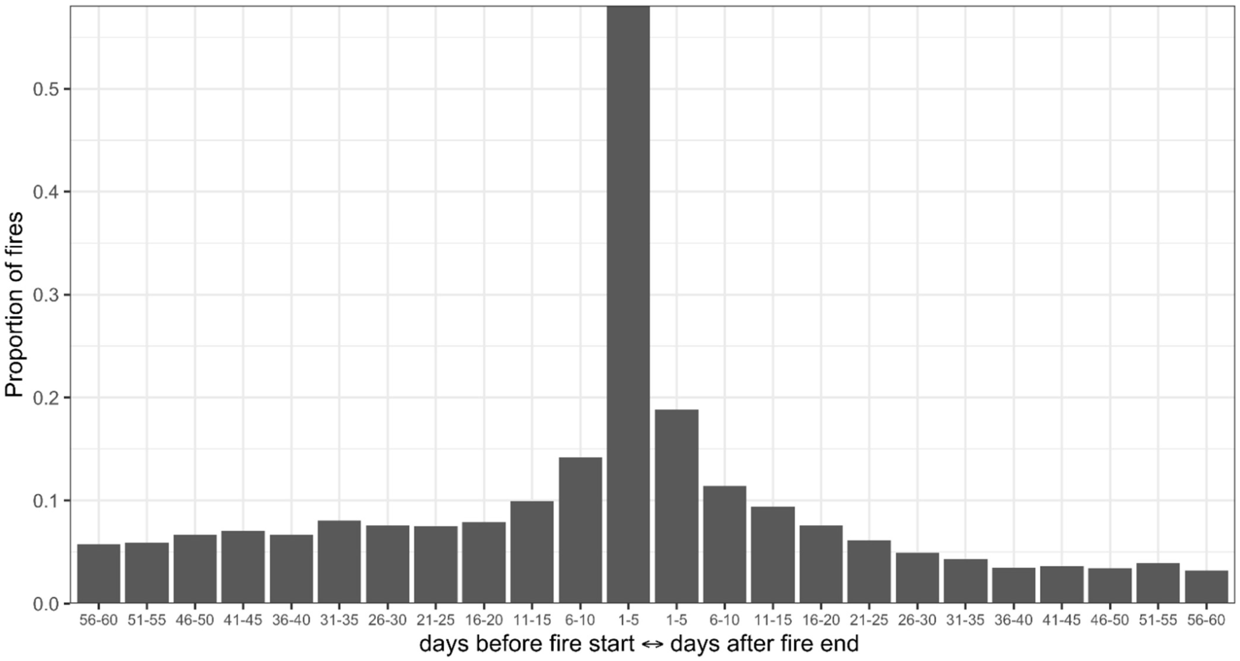
To compare satellite data to our ground-based fire perimeters we had to assign individual satellite fire detections to specific known fires. Satellite fire detections were assumed to be associated with a fire if they were within 1 km of the final fire perimeter and within a temporal window (45 days before, and 15 days after) surrounding the start and end dates of that fire’s perimeter data. We used a temporal window with relatively wide margins to avoid excluding fire detections due to delays in fire incident reporting or lingering hotspots due to smoldering combustion after an incident is closed (see Appendix A for details on window selection). 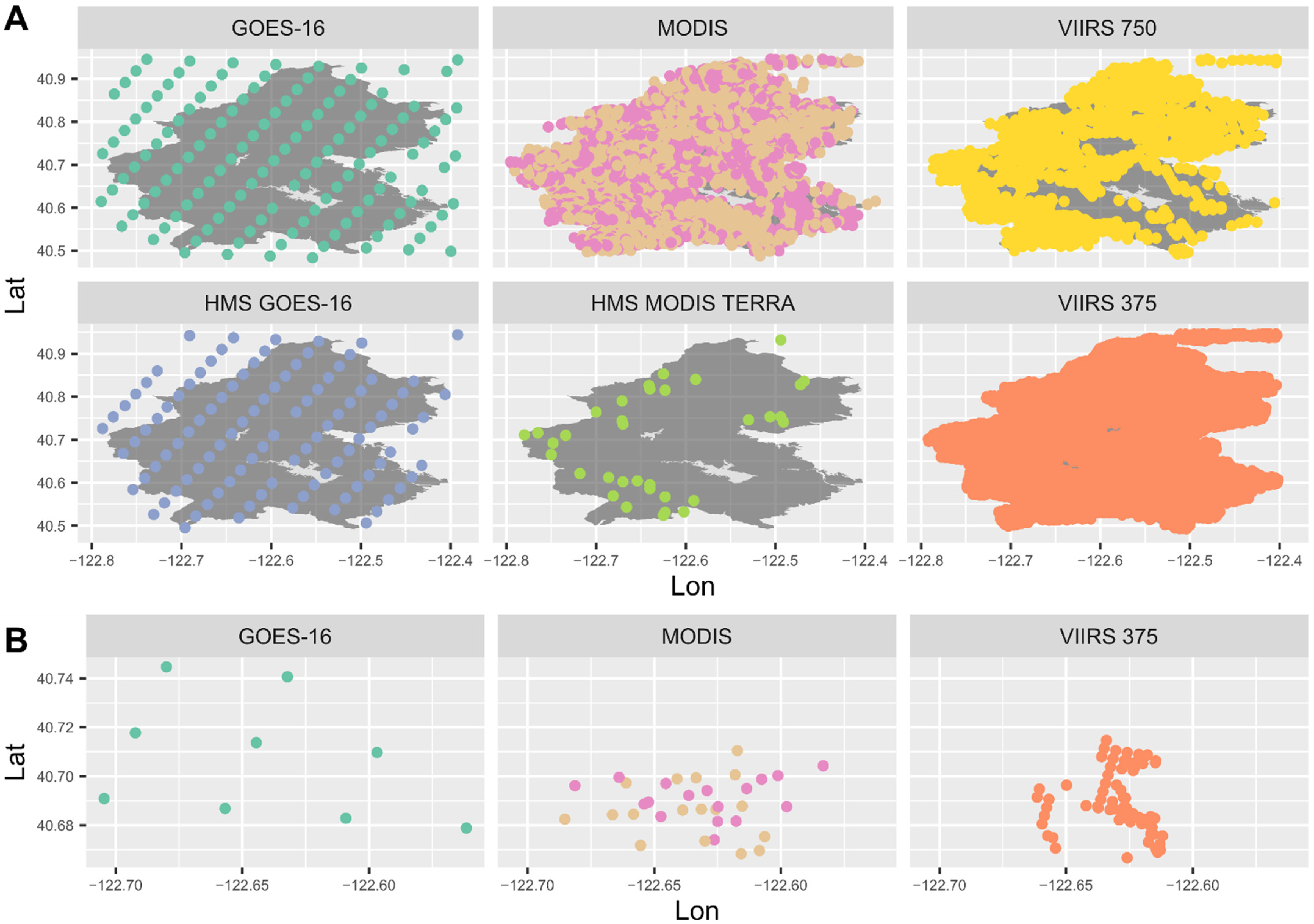Figure 1 shows an example of the fire detections within our temporal window which were assigned to the 2018 Carr fire in California.

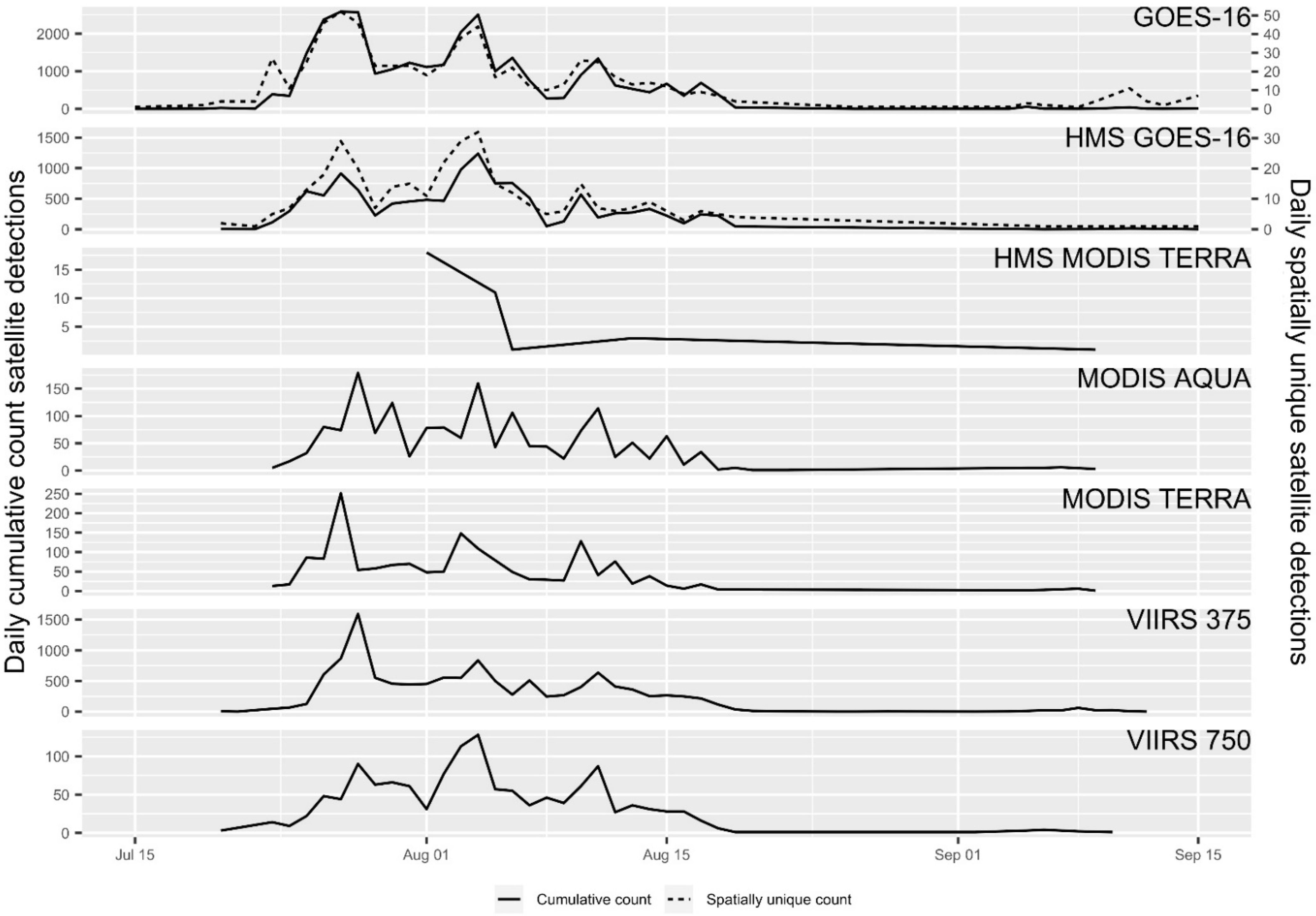
2.2.2. Summarizing Assigned Satellite Fire Detections

Satellite fire detection products differ in spatial (Figure 1B) and temporal resolution (Figure 2). To account for these differences, assigned satellite fire detections were summarized into counts for model fitting using two methods. The first was a cumulative sum of all associated fire detections by satellite source, while the second was a daily cumulative sum of spatially unique points. In the latter method, the cumulative sum of all fire detections was reduced to daily spatially unique locations only, i.e., in calculating a cumulative sum of fire detections, each unique lat/lon pair is counted only once per day. For single-pass polar-orbiting satellite data (e.g., MODIS Aqua), these two methods are identical; however, the two methods differ substantially for geostationary platforms. Figure 2 shows an example of the daily fire detection counts from these two methods for the Carr fire. The use of daily spatially unique counts serves as an attempt to help rectify differences in the number of detections occurring on different days due to non-fire influences such as intermittent obscuring clouds. We note in Figure 1A and Figure 2 the lack of HMS MODIS Terra fire detections. While we can only speculate as to why, this could be due to the operational real-time nature of the HMS fire detection dataset.

2.2.3. Final Training and Validation Datasets

Fire incident data, now with summarized fire detection information, were segregated into training (2017–2019) and validation (2020) datasets based on year. The training dataset contained 2699 fire incidents with assigned satellite fire detections, amounting to 61% of all of the fires in the GeoMAC dataset for this time period. Fires which were not detected by the satellites tended to be smaller than those that were detected (average acres of 104 vs. 7038). The validation dataset contained 401 fire incidents with assigned satellite fire detections. Overall, our datasets contained an average of 775 fires per year (401–1022) with an average of 6.7 million acres burned per year (4.0–8.1 million). Individual fires ranged from as small as 0.004 acres to over 650,000 acres.

Finally, each fire incident in the training and validation datasets were assigned a vegetation group from Table 2. Vegetation groups were assigned based on the vegetation type that covered the majority of the fire perimeter area.

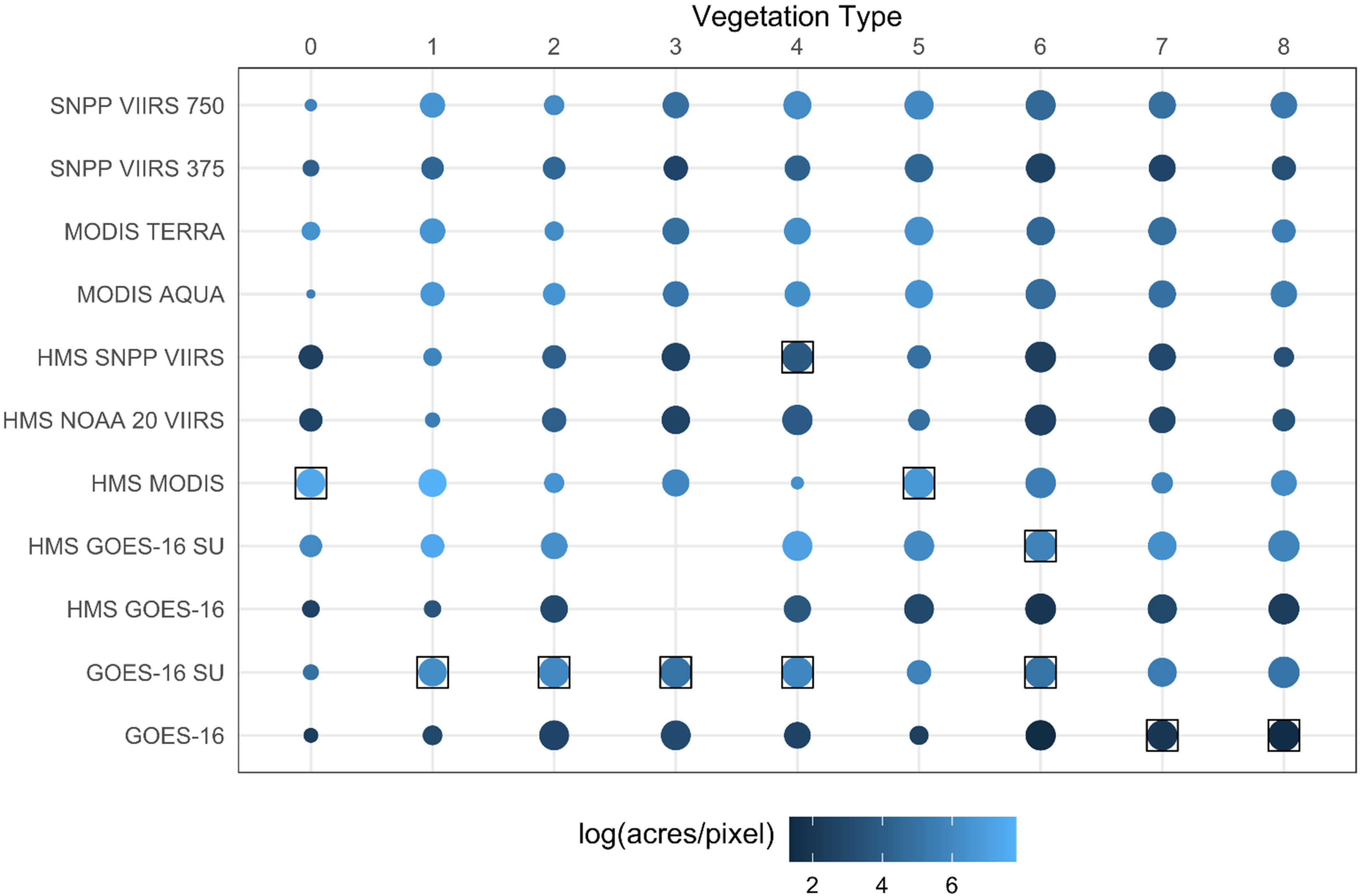
2.3. Fitting Burned Area Estimation Models

With the fire incident training dataset outlined above, we developed a series of statistical relationships for each satellite product (Table 1) for each vegetation type (Table 2) relating total burned area to the two different methodologies for aggregating fire detections—(a) the cumulative number of detections; and (b) the cumulative number of daily spatially unique detections (see Appendix B for details on intermediate models). Each model was a single variable linear regression model of the following form:

Burned Area_veg,source = β * Detections_veg,source

(1)

For fires in vegetation group veg = (0, …, 8) a model was fit using fire detections from each satellite source = (HMS GOES-16, HMS SNPP VIIRS, HMS NOAA 20 VIIRS, HMS MODIS Terra, GOES-16, MODIS Terra, MODIS Aqua, SNPP VIIRS 375 m, SNPP VIIRS 750 m). Since each model is a zero-intercept linear regression model relating burned area (Burned Area) and fire detections (Detections), β represents acres per fire detection. Ultimately this produced 99 linear models ((9 cumulative detection counts + 2 spatially unique detection counts) × 9 vegetation ids). The HMS GOES-16/Decid. Shrub model, however, had data from only two fires, so was not further considered.

We compared and validated models via the modelled R², root mean square error (RMSE) of the observed and predicted values, and a cross-validation predictive R². We performed a cross-validation procedure which iteratively withheld ten percent of the fires in the dataset, fit the regression models using the remaining fires, and then predicted the burned areas of the withheld fires. This procedure was repeated 5000 times and the correlation between burned area and the model-predicted burned area was recorded with each iteration. The statistical significance of modelled R² between groups of satellite fire detection products (i.e., polar satellites vs. geostationary satellites) was tested via permutation tests with 100,000 random splits of modelled R² values. Observed differences in R² values from the permutation tests were compared via a 95% confidence interval.

2.4. Ensemble (ENS) Method for Estimating Burned Area

The models outlined above produce a maximum of 11 burned area predictions for a single fire incident (9 cumulative fire detection models and 2 daily spatially unique fire detection models). To use all of the satellite detection information collectively, but still arrive at one estimate, we evaluated several simple methods for summarizing the ensemble of burned area estimates: mean (ENS mean), maximum (ENS max), and median (ENS median). We evaluated each estimate via the same cross-validation procedure as before, but this time we calculated the mean, maximum, and median of all the burned area predictions for a withheld fire. With each iteration, in addition to correlation, we also calculated the mean absolute error (MAE) and mean absolute percentage error (MAPE) between burned area and the ENS mean, maximum or median burned area.

2.5. Tracking of Daily Burning Area

Using our models, we explored the utility of daily fire tracking. To do this we first selected known fires from the training dataset with at least five unique fire perimeters. This was done to ensure we selected fires which show growth progression over time. For each selected fire, we generated daily ensembles of burning area predictions by multiplying the model coefficients developed in Section 2.3 and the corresponding daily cumulative and spatially unique satellite fire detections from each satellite product for each day. We also calculated the daily ENS median to arrive at one burning area prediction per fire per day. We then compared the daily, where available, reported fire size to the cumulative predicted burned areas (cumulative sum of each daily predicted burning area). This was done for each satellite product separately as well as the ENS median.

3. Results & Discussion

We utilized collected fire size observations from GeoMAC and NIFC over the period 2017–2020 to examine how well a variety of satellite systems (Table 1) can estimate burned area, as well as the potential for using a combination of satellites to improve estimates.

Satellite fire detection products provide timely national coverage for estimating the amount of fire on the landscape, yet there are limitations to the use of satellites in burned area prediction. For instance, cloud cover or heavy smoke can obscure fires, preventing detection. Additionally, the satellite’s pixel footprint, which can vary from as small as 375 m (VIIRS) to over 2 km (GOES-16), and timing, from once-a-day overflights to continual geospatial observations, affect the minimum size and intensity of the fire needed for detection as well as contribute to uncertainty over the true spatial location of the fire.

As the satellite systems used here look at individual pixels at particular times, GeoMAC/NIFC fires are reflected in a number of distinct satellite fire detections (e.g., of adjacent or nearby points, or of the same points over multiple observation periods). By aggregating the satellite detections based on spatio-temporal overlap with the GeoMAC/NIFC fire perimeters, we can fit satellite specific models and test them against the incident reported fire sizes. Figure 3 shows an example of how well three of these models perform for a particular vegetation type (Ever. Tree), and show the wide variability in the number of fire detections from differing satellite products. The three models are able to explain 81% (MODIS Aqua model) to 92% (GOES-16 cumulative sum model) of the variance in burned area. These three models are generally a good representation of the other 99 models. All model coefficients and model fit results, including modelled R² and RMSE, from the 99 models are reported in

Table A3. Final model fits and performance results for models relating satellite fire detection products to reported burned area from GeoMAC fire incidents grouped by vegetation type.

Veg. Type	Number of Fires	Cumulative Count Model			Spatially Unique Count Model
		Coefficient	Modelled R2	RMSE	Coefficient	Modelled R2	RMSE
(a) HMS GOES-16
0	5	13.3	0.41	1574	457.8	0.61	1277
1	53	35.8	0.40	26,575	1629.5	0.66	20,079
2	124	20.4	0.81	16,299	573.6	0.78	17,720
3	2	NA	NA	NA	NA	NA	NA
4	88	38.4	0.80	22,410	1185.1	0.92	14,747
5	27	17.3	0.91	4665	438.4	0.93	4323
6	17	7.2	0.95	5605	298.4	0.99	2973
7	226	17.4	0.89	13,524	571.1	0.86	14,876
8	18	10.4	0.96	3034	340.1	0.97	2347
--	--	Avg. cross-validation R2 = 0.65			Avg. cross-validation R2 = 0.75
(b) HMS SNPP VIIRS
0	6	12.3	0.69	59
1	28	353.8	0.44	19,952
2	61	62.5	0.66	2270
3	69	14.9	0.85	4077
4	49	44.4	0.96	4542
5	20	139.1	0.65	3855
6	27	12.0	0.96	3989
7	280	18.3	0.81	13,392
8	26	27.6	0.52	1617
--	--	Avg. cross-validation R2 = 0.76
(c) HMS NOAA 20 VIIRS
0	5	15.5	0.64	69
1	30	250.6	0.31	21,424
2	61	58.5	0.69	2178
3	67	14.6	0.85	4050
4	52	46.9	0.93	5504
5	17	121.9	0.57	4628
6	21	12.5	0.96	4335
7	285	17.9	0.78	14,292
8	25	32.2	0.62	1466
--	--	Avg. cross-validation R2 = 0.75
(d) HMS MODIS TERRA
0	5	1591.6	0.86	3805
1	62	2520.1	0.84	18,924
2	175	666.8	0.51	45,054
3	72	389.9	0.81	5481
4	118	585.5	0.22	42,024
5	24	802.4	0.96	3196
6	26	255.6	0.94	7070
7	677	352.7	0.57	23,948
8	32	452.6	0.75	16,152
--	--	Avg. cross-validation R2 = 0.56
(e) GOES-16
0	16	9.8	0.30	1075	142.1	0.34	1038
1	123	18.0	0.50	16,235	528.2	0.85	8830
2	200	15.7	0.91	5861	424.1	0.94	4724
3	5	20.6	0.91	141	161.9	0.95	102
4	195	14.2	0.78	16,191	380.6	0.96	7051
5	39	11.7	0.47	3811	299.6	0.69	2916
6	27	3.8	0.93	5545	163.8	0.99	2294
7	361	7.5	0.92	8808	241.7	0.88	11,131
8	20	4.3	0.99	1627	167.9	0.98	2097
--	--	Avg. cross-validation R2 = 0.75			Avg. cross-validation R2 = 0.88
(f) MODIS AQUA
0	20	274.3	0.06	5020
1	105	785.3	0.68	21,533
2	233	699.1	0.61	35,306
3	98	165.0	0.74	5437
4	164	522.2	0.74	20,656
5	45	621.6	0.84	5241
6	48	106.0	0.93	5642
7	798	143.7	0.81	14,426
8	45	246.2	0.78	12,915
--	--	Avg. cross-validation R2 = 0.71
(g) MODIS TERRA
0	14	601.9	0.45	4598
1	94	696.8	0.73	20,323
2	235	469.3	0.48	40,442
3	108	123.9	0.78	4785
4	167	519.7	0.79	18,695
5	36	566.8	0.86	5435
6	40	83.5	0.85	9008
7	807	129.1	0.84	13,449
8	41	250.8	0.65	16,641
--		Avg. cross-validation R2 = 0.71
(h) SNPP VIIRS 375 m
0	28	61.6	0.38	3470
1	167	80.7	0.62	18,703
2	391	83.5	0.62	26,809
3	139	15.7	0.69	5037
4	265	67.9	0.74	16,496
5	82	82.2	0.85	3707
6	87	13.6	0.89	5163
7	1080	16.3	0.80	12,990
8	65	28.5	0.68	12,674
--	--	Avg. cross-validation R2 = 0.70
(i) SNPP VIIRS 750 m
0	20	311.2	0.19	4673
1	102	677.4	0.72	20,316
2	280	451.5	0.52	35,537
3	98	129.4	0.77	5198
4	180	457.4	0.84	15,755
5	55	415.0	0.88	4070
6	58	95.4	0.92	5522
7	858	135.4	0.81	14,111
8	48	191.1	0.78	12,335
--		Avg. cross-validation R2 = 0.71

or visually shown in Figure 4.

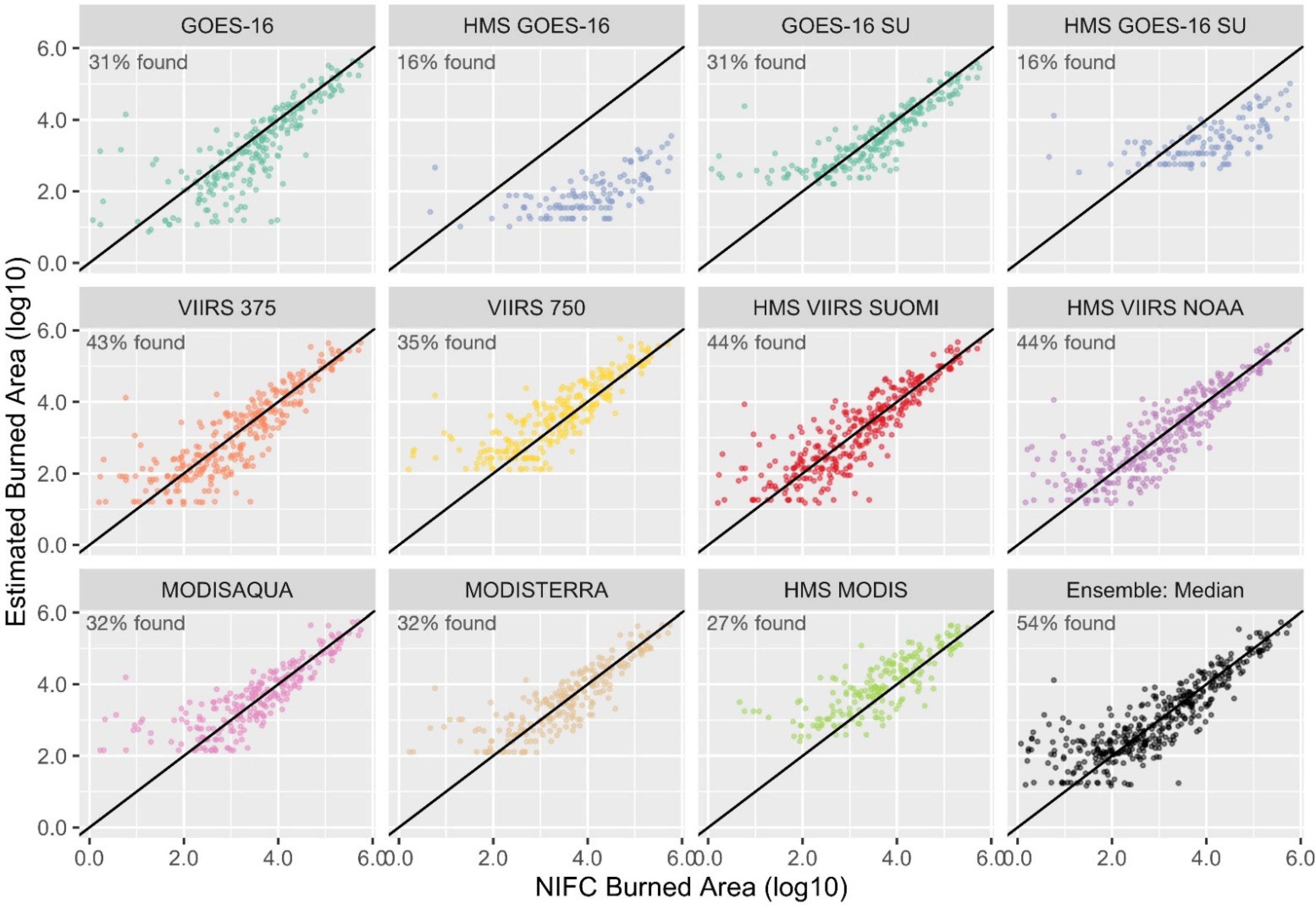
3.1. Modelling Total Burned Area: Overall Performance

While the various satellite fire detection products each detect the bulk of the overall fires that occurred in any given year, and while the overall patterns of regional variability and interannual variability can be found in each, there are substantial differences in how well each satellite performed. Overall, the geostationary products performed better (R² = 0.80 on average) versus polar orbiting products (R² = 0.71 on average), highlighting that their ability to catch the apex of a fire’s intensity throughout the day can offset their generally coarser sensor pixel resolutions. This difference was further found to be statistically significant following a permutation test. Looking across vegetation groups, the products from GOES-16 (HMS and original source) had the best model performance (R² = 0.84) (Figure 4). Additionally, GOES-16 daily spatially unique cumulative sum models have the highest predictive R² (R² = 0.88) of all models (Table A3).

In most cases, there are only small differences between model fits using the two fire detection counting methods (Table A3). The daily spatially unique cumulative sum models, however, perform better on average than their cumulative sum models counterparts in cases where the two models result in different model fits (e.g., GOES-16) (average R² = 0.84 vs. average R² = 0.76).

Performance varied substantially across vegetation types. Grouping broadly, fires located in sparse or limited vegetation are the worst modelled (R² = 0.45 on average); this vegetation group also has the least number of fires available for model fitting (on average of 13 fires per model), making its performance more suspect. The next best modelled are fires found in grasslands (R² = 0.65), followed by shrublands (R² = 0.80). Fires in treed areas performed the best (R² = 0.85), with the deciduous tree vegetation type topping the list (R² = 0.94). This result matches with previous studies, as lighter fuels and faster fires found in grasslands have been shown to be harder to capture by satellites [18].

Our results were confirmed in examination of model performance on additional data obtained for calendar year 2020. A separate validation dataset provides an opportunity to assess model performance on unknown fires and provide an unbiased estimate of model skill. Overall, correlations between burned area predictions and reported burned area for fires in 2020 are quite good. The average correlation across all models is 0.83, and predictions generated from the GOES-16 daily spatially unique model have the highest correlation (r = 0.90). Initial analysis of fires in 2021 (the first year this system was put into real time use) showed largely similar results, but this will be analyzed further in future work.

3.2. Tracking of Daily Burned Area

In addition to the overall number of fires and overall burned area, applications such as incident management and smoke forecasting use satellite systems for their ability to track the growth of an individual fire. To understand how these systems may benefit from our models, we emulated the fire information needed by these systems to estimate daily fire emissions by “tracking” daily burning area estimates. Smoke forecasting models require daily measurements of active burning, which, is not readily available. Using our models trained on total burned area, we examine how well they predict active burning by generating daily predictions of burning area for a subset of fire incidents from our training dataset. We selected fires with at least five unique fire perimeters, which resulted in 678 fire incidents. Over the lifetime of the selected fires, we used the model coefficients (Table A3) and the daily cumulative and spatially unique fire detections from each satellite product to produce daily burning predictions. We present the following results as indicative and not conclusive as we tested with a subset of fires from our dataset.

The geostationary products, again, performed better (predictive R² = 0.93 on average) versus polar orbiting products (predictive R² = 0.79 on average). Predictions generated from GOES-16 (the cumulative fire detection model) once again have the highest correlation of any satellite product (r = 0.95; predictive R² = 0.90). Overall, the average correlation between daily incident reported burned area and model predicted burned area across satellite products is 0.84 (predictive R² = 0.73).

Fires located in sparse or limited vegetation are again the worst modelled (predictive R² = 0.04), however, this result was based on only three fires. The next best vegetation types are treed (predictive R² = 0.84), and then grasslands (predictive R² = 0.86). Shrubland areas performed the best (predictive R² = 0.92).

3.3. Modelling Total Burned Area: Ensemble (ENS) Approach

There are several reasons for using fire detection information from multiple satellite products, such as taking advantage of different spatial and temporal resolutions and leveraging the strengths of both geostationary and polar platforms. In addition, other issues with satellite detections, such as false detections, may be mitigatable by looking across different satellite systems. The satellite instruments themselves also differ in sensitivity, and must compensate for changes in pixel size and shape and on the scan angle of detection. For these reasons and others, having an ensemble of burned area estimates from multiple satellite products is preferable.

To use all of the satellite detection information available, we developed several simple statistical approaches to summarize the results across the different satellite products and models. It should be noted that we used all of our information, including HMS, though an ensemble could easily be done with just the original source datasets. We performed a cross-validation procedure with fires from the training dataset taking the ENS mean, median, and maximum of burned area estimates, and the results for each were very similar. The average predictive R² is 0.74 for the ENS median, 0.75 for the ENS mean, and 0.75 for the ENS maximum. We choose to continue to use the ENS median as the representative burned area estimate going forward because it is less likely to be unduly influenced by extreme model predictions (like mean and max), and the ENS median represents an actual total burned area prediction produced by a model. The average mean absolute error (MAE) from the cross-validation is 3641 for the ENS median, while the average mean absolute percentage error (MAPE) is 51.4. The median MAPE, however, across all cross-validation iterations is 35.7. This difference is likely due to the biased nature of MAE and MAPE to large outliers.

We also applied the ENS median to total burned area predictions of fires during 2020. The correlation between total burned area and the ENS median of model predictions is 0.90, which is higher than the average correlation across satellite products. The MAPE between total burned area and the ENS median is 12.2. For 2020 fires with reported burned areas at least 1000 acres, the correlation with the ENS median is 0.89 and the MAPE is 0.65, while fires with burned areas less than that is 0.27 and 22.6, respectively. In fact, we found that the MAPE between burned area and the ENS median tends to decrease as fire sizes get bigger. This all suggests that the ensemble performs significantly better for fires of at least moderate size. This makes sense given the interpretation of the linear regression models (model coefficient = acres per fire detection) where even if a small fire is detected by a satellite, the total burned area is predicted, at minimum, to be 3.8–298.3 acres depending on which satellite detected it. The 50th quantile of reported burned area of fires in 2020 is only 60 acres, making it much more likely for the ensemble to over-predict these smaller fires, as reflected in its poorer correlation and MAPE.

3.4. Using the Ensemble (ENS) for Daily Tracking of Burned Area

We calculated the ENS median of up to 11 possible daily burning area estimates for a subset of 678 fire incidents from the training dataset (see Section 3.2). The correlation between daily reported burned acres and the ENS median was 0.90 (predictive R² = 0.82). Which again, like was the case when testing the ENS median on 2020 fires, is higher than the average correlation across satellite products. This further suggests that using information from all the model predictions to arrive at a single burned area estimate is of great value, particularly for multi day fire growth events. This strong correlation suggests that using our model ENS to estimate burning area in a near real-time framework, similar to the needs of smoke forecasting models, would be encouraged and successful.

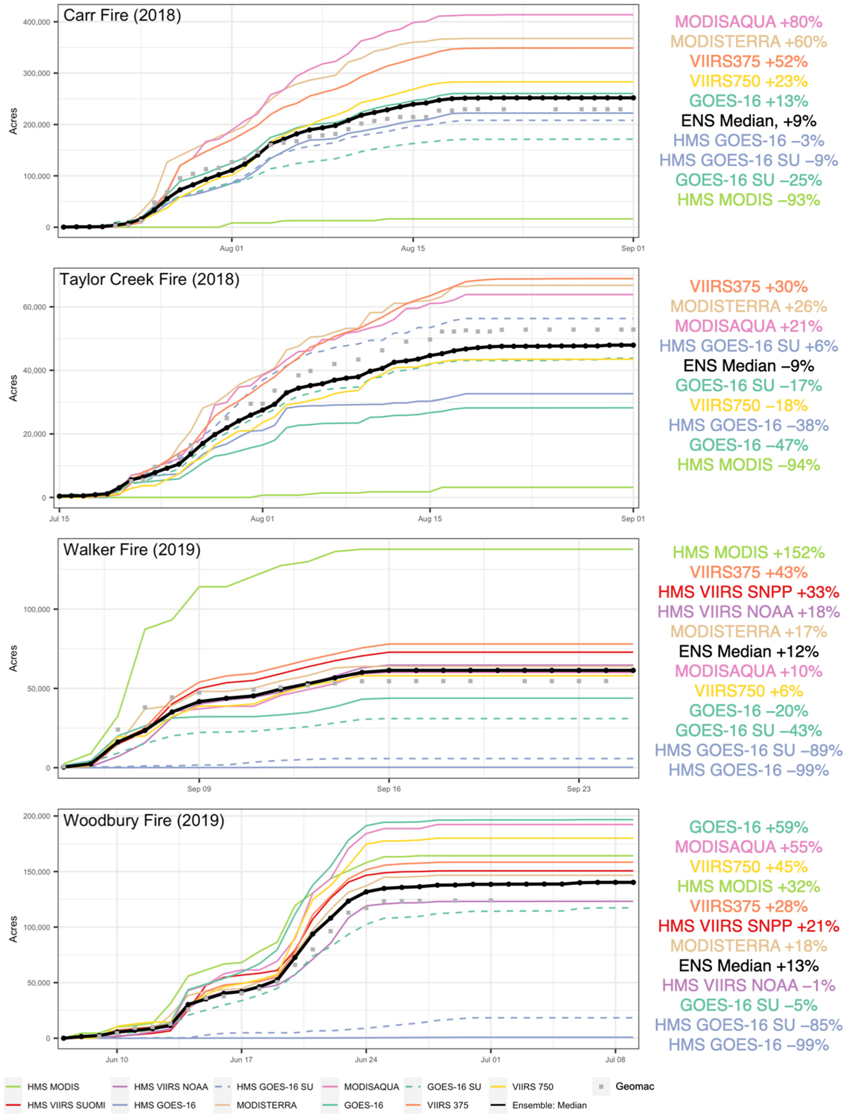
We further chose to highlight daily burning area tracking for the Carr and Taylor Creek fires (2018), as well as the Walker and Woodbury fires (2019). We chose these fires for their moderate to large sizes and breadth of satellite source options in the ENS. The daily burned area tracking results for these fires are shown in Figure 5.

Interestingly, the satellite product that best represents the progression of area burned is different for all four fires (Figure 5). The Carr fire is best represented by the HMS GOES-16 models (under predicted by 3 and 9%); the Taylor Creek fire is extremely well represented by the ENS median and HM GOES-16 spatially unique model (under predicted 9%, over predicted 6%, respectively); the Walker fire is best represented by the SNPP VIIRS 750 m and MODIS Aqua models (over predicted by 6 and 10%, respectively); while the Woodbury fire is best represented by the HMS NOAA 20 VIIRS and GOES-16 spatially unique models (under predicted by 1 and 5%, respectively) (Figure 5). Some models over-predict total burned area, while others under-predict, but these are not consistent across the four fires. For example, the HMS MODIS Terra fire detection model significantly over-predicts the size of the Walker fire, but significantly under-predicts the size of the Carr and Taylor Creek fires. The ENS median is in general a good predictor of total burned area for all four fires (within 9 to 13% of the reported burned area) (Figure 5), which is a reassuring result as there is no single satellite fire detection product that consistently provides the best results for all four fires. This further highlights the benefit of using information from the full ENS to produce more informed estimates.

4. Conclusions

This study examined the ability of satellite fire detection products to estimate the burned area of known fires and track their growth over time. Using fire detection data from multiple satellites, we developed burned area estimation coefficients for each of nine differing vegetation types over the U.S. for the period of 2017–2019. These coefficients were then tested with fires from 2020. The clear differential nature of the vegetation types and satellite products that we observed in our model fits and estimates led to the construction of an ensemble which samples information across all of the satellites to improve overall burned area estimates. This is particularly key as no single satellite product was found to best estimate burned area.

The modelling ensemble (ENS) we developed has shown enhanced accuracy with less data issues than individual satellites, and performs better in terms of model fit and predictive accuracy, as well as daily tracking of fire. Analysis of the robustness of this approach will benefit from additional data from future fire seasons as well as testing within real world applications.

Further work is underway to compare these results with FRP/FRE based estimates and to examine how well this methodology works in an operational capacity. For 2022, the ENS burned area estimates detailed here are being tested, with daily area tracking being used in a smoke forecasting system by the U.S. Forest Service led U.S. Interagency Wildland Fire Air Quality Response Program. While initial results show promise, examination of these estimates against other methodologies within this testbed system will provide a further validation of this approach.