Early Smoke Detection Based on Improved YOLO-PCA Network

Abstract

Early detection of smoke having indistinguishable pixel intensities in digital images is a difficult task. To better maintain fire surveillance, early smoke detection is crucial. To solve the problem, we have integrated the principal component analysis (PCA) as a pre-processing module with the improved version of You Only Look Once (YOLOv3). The ordinary YOLOv3 structure has been improved after inserting one extra detection scale at stride-4 specifically to detect immense small smoke instances in the wild. The improved network design establishes a sequential relation between feature maps of lower spatial information and fine-grained semantic information in up-sampled maps via skip connections and concatenation operations. The testing of the improved model is carried out on self-prepared smoke datasets. In digital images, the smoke instances are captured in various complicated environments, for example, the mountains and fog in the background. A principal component analysis (PCA) helps in useful features selection and abandons the involvement of redundant features in the testing of the trained network hence, overcoming the latency at inference stage. In addition, to process small smoke images as positive samples during training, new sizes of anchors are calculated on small smoke data at a specified Intersection over Union (IoU) threshold. The experimental results show the improvement in precision rate, recall rate, and mean harmonic (F1-score) by 2.67, 3.06, and 5.59 percentages. The respective improvements in average precision (AP) and mean average precision (mAP) are 1.66 and 2.78 percentages.

1. Introduction

Out of the many reasons for a country’s economic and social instability, fire incidents may be one of them that needs to be tackled at an earlier stage of its growth to avoid undesired damage to property and human lives.

It is impossible to eradicate fire hazards. However, accurate and timely detection of fire may reduce its damaging effects. Therefore, for fire safety applications, it is mandatory to develop the most reliable and fast response fire detection systems.

Among the various fire signatures, smoke is one of the most prominent characteristics of fire because it usually evolves earlier than flame [1]. Computer vision smoke detection systems easily detect a large or medium columns of smoke because of large pixel intensity values in digital images that are more distinguishable as compared to small smoke instances in the wild.

On the contrary, detecting small or light smoke in digital images is a challenging task where smoke features are indistinguishable from the complicated background. The detection of such smoke instances occurs if the network includes those features in training and testing. Therefore, a specific scale of detection must be added throughout the network specifically for the recognition of small smoke instances. In addition, to reduce the computational latency, the pre-processing module helps to filter out useful input features before feeding to the network.

For example, in [2], for the recognition of small objects in a complex environment, the feature maps are fused in a top-down and bottom-down fashion. The feature tensors present in the earlier layers of the network concatenate with later layers to combine the low-level information with highly refined semantic information. This modification is helpful to recover the information that may vanish in feature maps present at bottleneck layers of the network after extensive downsampling of the full-scale input images. In our improved design, the detection occurs at the four stages throughout the network instead of three-scale detection, and the fourth scale is added because of utilizing the small smoke information present in feature maps of resolution 104 × 104. The top-down fusion strategy establishes the sequential relation between the feature maps of 104× resolution and the maps on the top of the network downsampled by stride-4. The skip connections are inserted at the fourth scale to directly fuse the information of extensive small smoke instances present in high-resolution maps of dimensions 104 × 104, Figure 1. The upsampling of the maps, which are downsampled by stride-4, is necessary before the concatenation to recover the same spatial dimension as mentioned in [3]. This scheme enables a network to take leverage of comprehensive information fusion for small smoke instances. The high-level features in stridden maps and low-level features in high dimensional (104 × 104) maps are equally important for small smoke instances because they strongly influence classification accuracy and localization precision.

Figure 1. Schematic of the improved method. First, the principal component analysis transforms the random dimensions of smoke pixels into unique principal components in low space. The pre-processed co-related groups of pixels then feed into an improved version of YOLOv3 with an extra scale of detection.

Previous studies have also shown improvements in recognition of small smoke instances via feature maps fusion schemes for example, feature pyramid network (FPN) [4]. In FPN, the fusion of feature maps occurs either in a bottom-up or top-down fashion. The low-level spatial and refined semantic information is either concatenated or added by element-wise addition. The resultant feature maps can dramatically increase the detection accuracy of the network for small smoke instances.

For example, in [5], author verifies, the combination of feature maps has the potential to increase the overall detection accuracy of the deep neural networks, particularly for small objects. In [6], the low-level and high-level features were concatenated and added by using skip connections directly. They use a bottom-up module that downsampled the full-scale images by convolutional pooling with varying kernel sizes. The concatenated feature maps are normalized and used for final predictions. Another study [7] also adopts the fusion strategy. The pooling layers first downsampled the input images. A deconvolution module upsampled the processed images to regain the spatial dimensions. In [8], the author uses the lateral connections for the fusion of highly semantic and contextual feature maps from the top-down module and feature maps of general information from the bottom-up module. Their experiment also proves the effectiveness of those fusion schemes. In [9], they utilize a single shot multibox detector (SSD) and FPN. The original features of the SSD network fuse with the image features from the image pyramid network at four different scales. They fuse the features from current and previous layers for local spatial information.

The domain-specific anchors also increase the classification accuracy and localization precision of the network. The Intersection over Union (IoU) score would decide the positive and negative samples from the training datasets. If the ground truth boxes overlap with pre-calculated anchors at a given IoU threshold, the sample images of extra small smoke instances would be involved in the training process. It helps to improve the classification score and boost up the model’s generalization ability. Therefore, by running a clustering algorithm on a dataset of a small, medium, and large smoke instances, the anchors are calculated for each detection scale separately.

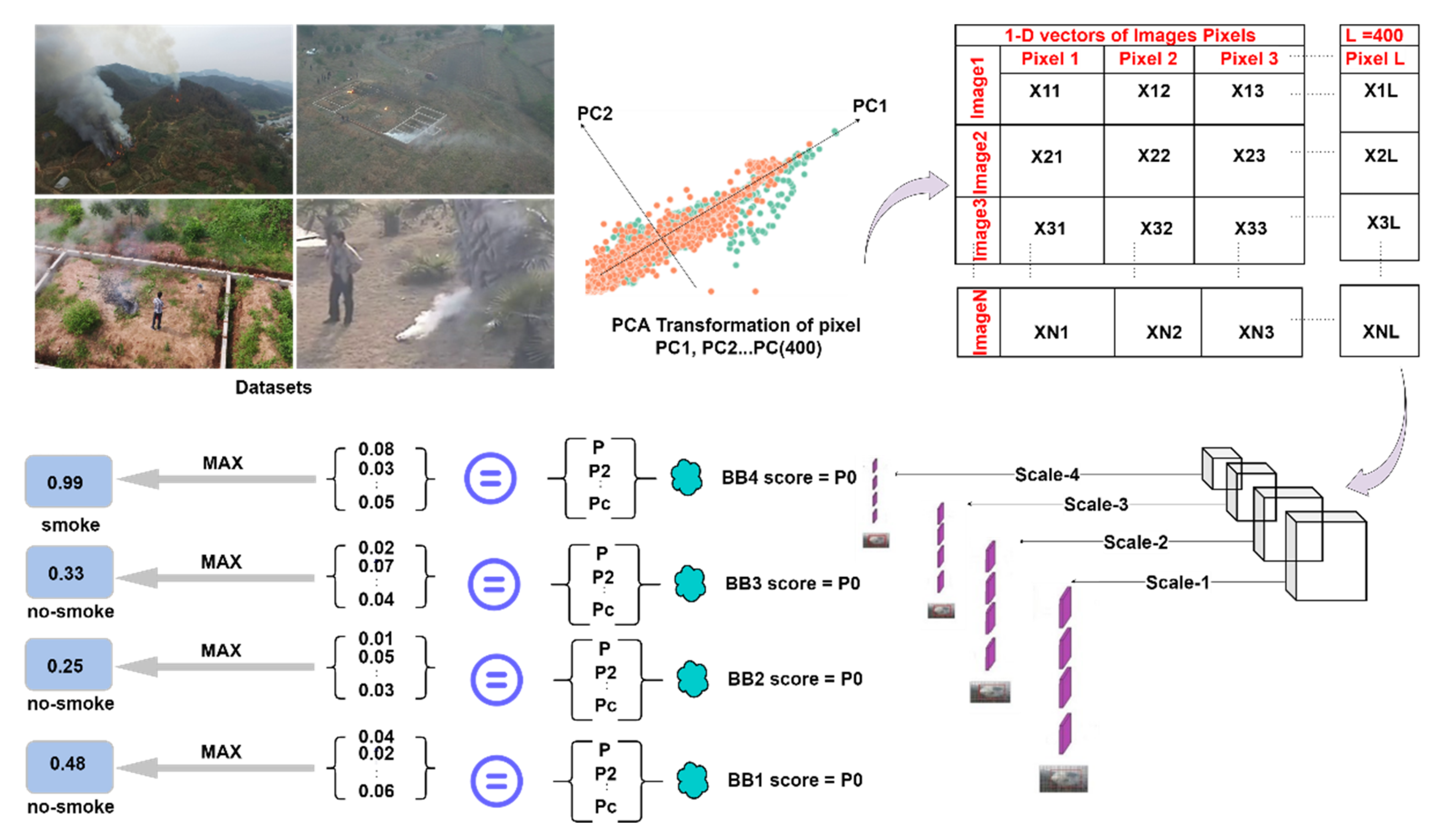
As part of the above-mentioned work, we integrate an improved version of a YOLOv3 with a pre-processing module named principal component analysis (PCA). The ordinary structure of the network expands up to four detection stages to avoid the information loss present at very earlier convolutional layers, while the numbers of anchor boxes for each detection stage are calculated precisely on the available dataset of small smoke instances. Due to the increase of the total number of detection scales, the total number of anchor boxes has also increased from 9 to 12 boxes, i.e., three boxes per scale. The computational cost of the improved network may increase after adding an extra detection scale for the fusion of feature maps in a top-down fashion. Therefore, principal component analysis as a pre-processing module is combined with the improved YOLOv3 to meet the real-time processing speed. Similarly, PCA is helpful to avoid the loss of information during backpropagation while updating the weights during training. An unsupervised PCA module also reduces the dimension of smoke data. Hence, it reduces the computational complexity present in the datasets. The network is more stable and deep enough to process higher-level semantic and contextual information concatenated with lower-level features of small smoke instances present in feature maps at the beginning of the network.

Figure 1 illustrates the flow diagram of the improved YOLOv3-PCA framework.

The motivation behind the network selection is that YOLOv3 [10] is lightweight and provides the best balance between accuracy and speed by predicting smoke at multi-scales through depth residual blocks (ResNet) [11].

YOLOv3 has a better inference time compared to YOLOv4 and is slightly less than YOLOv5 [12]. The integration of pre-processing PCA module with the improved YOLOv3 still makes it feasible to detect small smoke instances. YOLOv3 can generate the classification accuracy and positioning coordinates of the target in one step and uses the idea of multi-stage detection. Moreover, the mean average precision (mAP) of YOLOv3 is higher than SSD [13]. The purpose of the fourth scale in the traditional YOLOv3 structure is to compensate for the missed detections of positive samples of small smoke instances. The reason is that the spatial information in the feature maps of resolution 104× was ignored by the three-scale YOLOv3 structure. With the downsampling of the input images, the features related to small smoke instances may fade in low-resolution images. Therefore, it is required to consider those features present at the earlier layers of the network. The strategy helps to generalize a network so it can detect smoke instances at their evolving stages even in a complex environment.

More concisely, the following are our key contributions:

• We have improved a deep learning network, YOLOv3, to classify and localize small/light smoke instances in the wild. We inserted an extra detection scale at stride 4 to process the information of small smoke instances.
• To reduce the dimensional complexity present in the smoke datasets, we have integrated an unsupervised dimension reduction module principal component analysis (PCA) at the input of the improved YOLOv3. The input smoke and non-smoke images are pre-processed first before feeding the network.
• We have calculated the anchor boxes on smoke datasets for each detection scale separately. At the detection scales of 1, 2, 3, and 4 with strides 32, 16, 8, and 4, we have created the anchor boxes for large, medium, small, and extra small smoke instances.

The rest of the paper is arranged as follows:

In Section 2, we discuss the previous work carried out using convolutional neural networks (CNNs) and the respective improvements in the existing networks for the purpose of smoke detection. In Section 3, we briefly explain the improved design of the model and PCA as a data pre-processing module. Additionally, this section explains the full description of smoke datasets, their valid train-test splitting method, and complete working environment. In Section 4, we provide experimental results and a discussion of training and testing metrics. Finally, Section 5 concludes the manuscript.

2. Related Work

In previous work, many researchers used deep learning approaches to detect smoke as a sign of fire. The smoke detection based on texture and color information may not generate correct predictions. Many smoke detection methods based on convolutional neural networks are present in literature, for example, smoke segmentation, smoke detection, and integration of conventional machine learning methods with deep neural networks, i.e., hybrid systems.

2.1. Key Technologies & Networks Characteristics for Smoke Detection

Ref. [14] presents an improved dual-channel convolution neural network (IDCNN) specifically designed for the classification of smoke images. Two separate networks combine to build a whole architecture. The first CNN consists of max-pool and batch normalization layers. The second network uses the skip connection to fuse the feature maps for detailed information processing. The use of standard convolution increases the number of parameters that consequently slows down the training and testing of the model. This work presents an improved network replacing the operation of standard convolution with depth-wise and point-wise convolution. They compare the efficiency of both the original DCNN and the improved IDCNN. The use of depth-wise and point-wise convolution decreases the number of channels and, as a result, reduces the total learnable parameters of the network. The effect of network compression assists in reducing the total amount of calculation, improving the operating efficiency. They compared their improvement with DCNN and many other classifiers in terms of learnable parameters and the classification performance of the network.

In [15], the author presents a channel-wise and spatial attention mechanism combined with decision level and feature level modules. They redesign a lightweight CNN classifier, Visual Geometry Group (VGG16). They establish a smoke dataset having smoke samples in a fog environment and challenging negative examples. The attention mechanism helps to focus on smoke instances in severe fog environments. The feature level and decision level modules decide which feature maps carry information to fuse. Their network consists of three convolutional layers where the mid-layer is a deep layer. The network uses skip connections to combine low-level information with semantic information. The implementation of the framework can discriminate smoke from the fog in real-time.

Reference [16] implements a combined framework for smoke detection and segmentation in plain and hazy environments. A lightweight CNN network, EfficientNet performs the task of smoke detection and atrous convolution-based DeepLabV3+ segments the smoke pixels. The structure of EfficientNet makes it feasible to use for smoke detection on memory-constrained devices. The main building block of the detector is mobile inverted convolution layers with squeeze and excitation modules. The attention module is helpful to distinguish smoke in the haze. The semantic segmentation is performed on the output maps of EfficientNet by DeepLabV3+ followed by a softmax classifier. The architecture of DeepLabV3+ utilizes an encoder-decoder structure with depthwise separable convolution for semantic segmentation and softmax as a classifier to classify the individual smoke pixels. Their experiment shows a notable gain in detection results with a decrease in false alarm rate. Additionally, they report an increase in the global accuracy and mean Intersection over Union value for the segmentation module.

Ref. [17] implements a novel unsupervised approach for discrimination and mapping of smoke patterns based on the linear hyper-spectral un-mixing technique. Smoke is a non-rigid object of deformable shape with a highly variable degree of transparency and atypical motion. Therefore, the typical descriptors may fail for accurate detection of smoke as they map only low-level visual features of smoke. Along with the visual attributes of smoke, they suggest a new feature space and feature mapping to learn the smoke pattern. Using the un-mixing approach, they map smoke features in the new feature space where the vertices of the minimum volume simplex, which encloses all image pixels, represent the new axes. They formulate the feature mapping as an optimization problem to find the vertices of the minimum volume enclosing simplex as new axes of new feature space. The similar smoke attributes constitute some new axes with large coordinate values while others with low coordinates represent non-smoke axes. Their approach has the potential to discriminate smoke regions from non-smoke patterns.

Ref. [18] implements a hybrid smoke classification system based on domain knowledge. First, they segment and extract the suspected smoke regions from video frames. Then, a CNN classifier employs to discriminate the smoke regions from smoke-like regions. In the first stage, the author uses the Gaussian Mixture Model (GMM) to subtract the static background and extract the moving smoke as a foreground. GMM extracts the motion vectors of smoke and separates the smoke instances from the complex scenes. The employed framework effectively classifies image patches of smoke instances from non-smoke objects by a deep neural network.

We present the above studies to argue that the employed modifications may increase the detection performance only. However, we explore another aspect of research where the combination of traditional feature extraction methods and deep neural networks, i.e., hybrid systems. Our findings explain, the hybrid systems have the following benefits in the domain of smoke detection: (a) the dimensional complexity of input data reduces, (b) boost-up the generalization strength of the trained model, and (c) decreases the latency and increases the inference speed.

2.2. Generalized Deep Networks in Smoke Detection

Low-dimensional feature maps are less computationally expensive to process. Therefore, the deep layers of the neural network downsample the input images into number of channels. This downsampling may lose the related information of small smoke instances because of continuous reduction in spatial dimensions. In the literature, various techniques are present to preserve the low-intensity features of small smoke instances. Here, we summarize those methods in four categories as:

Firstly, the improved convolutional kernel operations have the potential to boost up the performance of the network for the recognition of small smoke instances. For example, the increase in kernel sizes may increase the network’s receptive field, which is helpful to process the contextual information of the small smoke instances. Secondly, top-down or bottom-up modules are employed to fuse the processed feature maps with high-resolution feature maps. Thirdly, the network may restrict extensive downsampling by substituting the residual blocks to process the features. In the last option, the implementation of dataset pre-processing module is also helpful; for example, small smoke instances are augmented. Hence, the datasets are more diverse, e.g., scale transformation [19], and scale-dependent pooling [20].

For small-scale networks, the use of expanded convolution is not feasible because it can degenerate the performance, and the convergence effect of the network may reduce up to 3% points as mentioned in [21]. In [22], they replaced a two-step downsampling convolution block in YOLOv3 by double-segmentation and used a bilinear upsampling module for features amplification. Additionally, they resolved the problem of gradient fading by adding a residual network block at the output layer that is helpful to increase the number of feature maps for small object detection. The mentioned modifications may improve the detection performance for small smoke instances but the inference time complexity issue is not addressed.

Similarly, [23] uses improved YOLOv3 and increases the number of detection scales from three to five by adding two more convolution blocks to form a five-stage feature pyramid structure. To capture and transfer the features of small objects conveniently, they integrated a dense block. In [24], they improved the feature fusion tendency of the YOLOv3 by concatenating the low level and high-level features without increasing the number of detection scales. They fused the feature maps of different resolutions at three arbitrary scales to detect large, medium, and small objects. The training scheme of the improved network is transfer learning that alone cannot address the problems of gradient fading in a deeper network. Additionally, the solution of the problem of time complexity is not mentioned.

In [25], the authors redesign the network from three-scales detection to two-scales detection. They reduced the image downsampling by removing the convolution blocks. Their method is suitable to attain a high speed of inference, but the accuracy is comparatively low. Moreover, they fused the spatial information of a small object with the deep feature maps by concatenation and up-sampling at the scales 1 & 2 with strides 32 and 16 only. This scheme is feasible for fast detection but cannot capture the encoded information of immense small objects present in high dimensional maps. In [26], the authors suggested a transfer learning-based solution to increase the detection speed of the network. They used a K++ means clustering algorithm to revise the anchor boxes. They performed a multiscale fusion of feature maps at three scales with strides 32, 16, and 8. They focused only on the training strategy without considering deep feature fusion at more than three scales to include the basic low-level information of the target object. Therefore, this strategy may improve the convergence rate of the network but not the detection accuracy for small smoke instances.

3. Methodology

In this section, we present an improved design of the base model and the implementation of PCA as a pre-processing and feature extraction module. Meanwhile, we describe the working of PCA integration with the tuned version of YoloV3. The dataset introduction, train-test split methods and entire working environment have also been presented here.

3.1. Improved Design of the Base Network

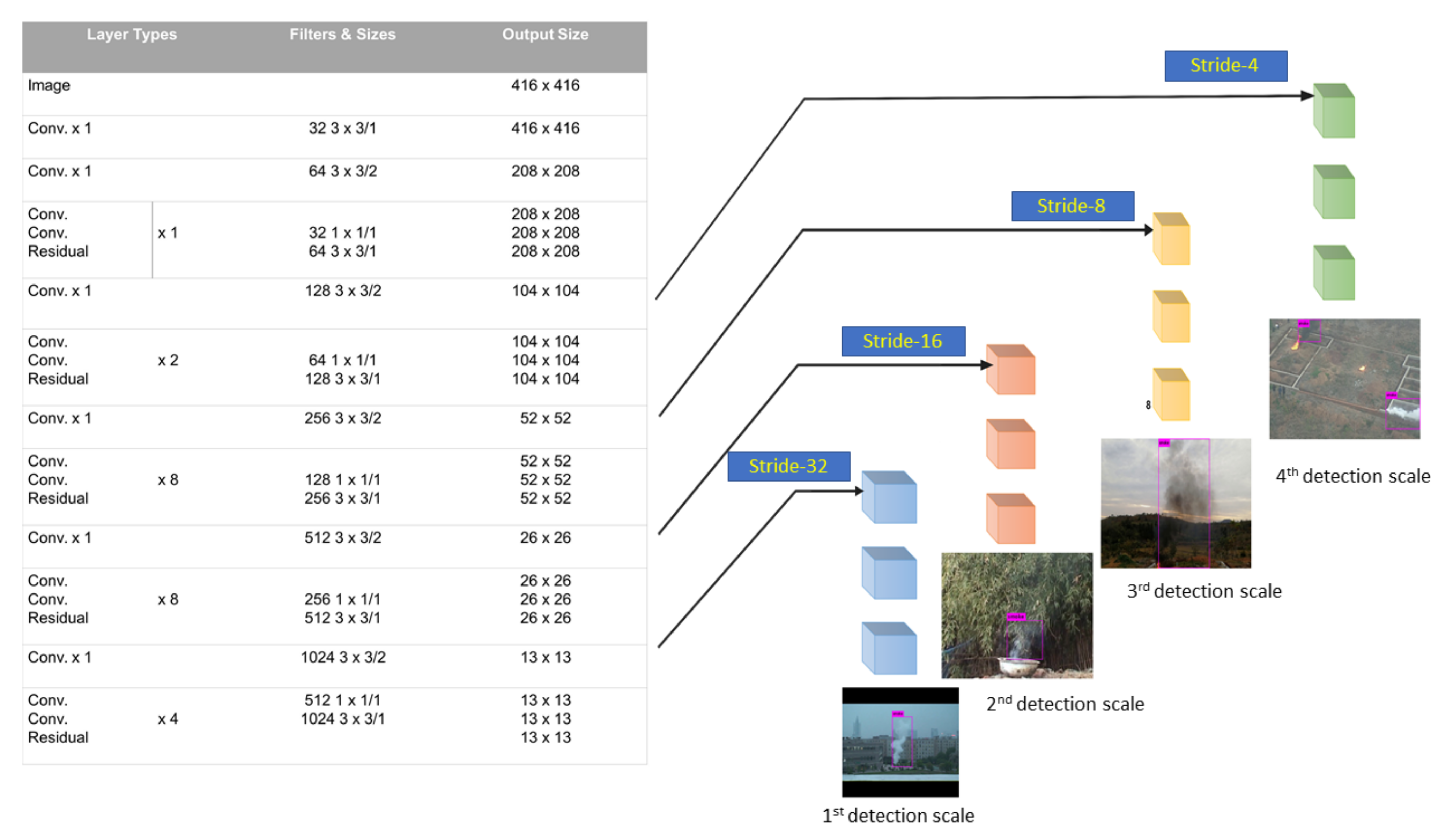
Instead of three-scales traditional YOLOv3, we implemented a four-scales improved architecture of YOLOv3 to detect particularly extra small smoke instances in the wild. The detection performance of an extra-scale improved network is comparatively high due to the fusion of the downsampled maps at scale-4. Downsampling at stride 4x produces a greater number of feature maps of a full-scale image, which are combined with the feature maps of resolution 104 × 104 at detection scale-4. In addition, the smaller grid cells of size 104 × 104 have large receptive fields that can detect the minute features of small smoke instances. Figure 2 shows the improved design of the network.

Figure 2. The structure of 4-scales YOLOv3 network. Scales 1, 2, 3, and 4 detect large, medium, small and immense small/light smoke instances in the wild with strides 32, 16, 8, and 4 respectively.

The increase in detection scales brings scale diversity in the feature maps of various sizes. This improvement considers the very low-level spatial information with the high-level semantic information at scale-4 that increases the recognition efficiency of the detector. Because pixel intensities of small smoke instances are smaller enough. The 52 × 52 sized grid cells cannot capture those pieces of information fully, but adding one more detection scale with grid sizes 104 × 104 can process those extra small pixels efficiently.

Moreover, there are three bounding boxes for each grid cell. Adding an extra scale will generate more bounding boxes. Thus, the network can accurately predict the bounding box coordinates around small smoke instances. A 2D-upsampling layer is programmed to recover the spatial dimension of 104 × 104 deep processed maps. The use of skip connection between two-level pieces of information can avoid the gradient disappearance problem and process the information in a feed-forward manner. The concatenation of feature maps occurs at scale-1, 2, 3, and 4.

3.2. PCA Implemenatation & Calculation Process

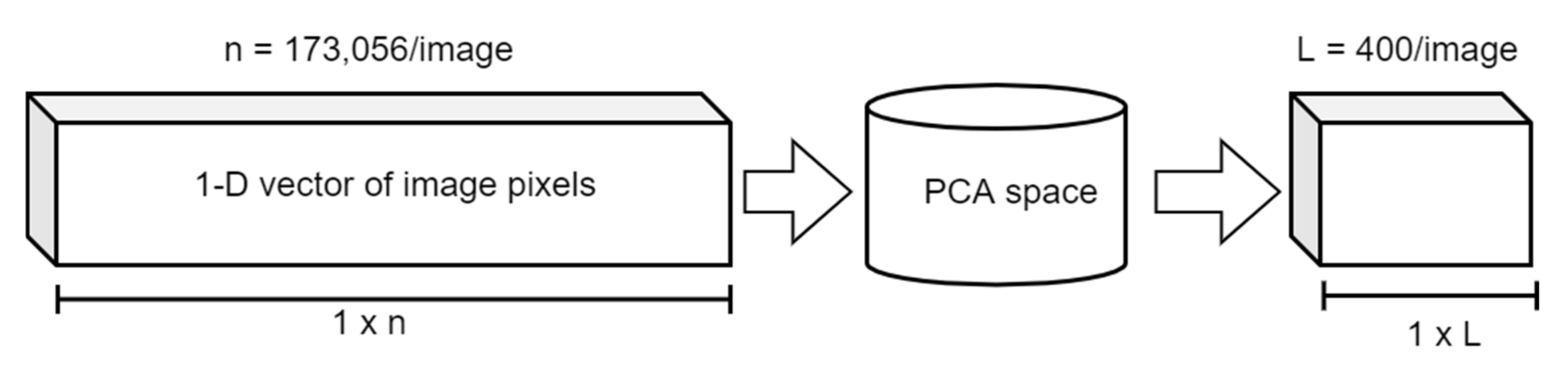
PCA is a popular unsupervised algorithm in the field of image processing. It is basically used for dimensionality reduction of image datasets, which actually reduces the size of feature vectors for object recognition or classification of images. PCA can be implemented either by using eigenvalues decomposition (EVD) or by using singular value decomposition (SVD). Before implementing a PCA algorithm, data is transformed into a single vector representation by a hot vector encoding scheme, and then PCA space reduces the dimension or size of this single vector as shown in Figure 3.

Figure 3. Single vector demonstration. Initially, pixels are thousands in numbers and randomly co-related. Later, the PCA space reduces the length of the pixel vectors to 400 only. Those 400 principal components represent the unique dimensions for groups of highly co-related pixels.

In a raw dataset, the pixels of the image as variables are randomly arranged in the XY plane where each data point is represented by a large value of X and Y. These data points are highly correlated. This correlation can be observed if data points are viewed from a highly informative viewpoint in the direction of a new principal vector u. This vector line in the direction of data points with another orthogonal vector line v formed a new axis system called the principal axis. we can achieve a more compact representation of the same data along with this new principal axis system. The origin of this new axis system is located at the mean of datapoints on the XY plane. Hence, the covariance of data along this new axis system is much smaller to zero. It means the PCA finds the new axis system which is defined by the principal directions of variance of a given set of data. The prime goal of dimensionality reduction can be achieved by reducing the variations of data along the v axis line. In this way, all datapoints would be assumed in the direction of the u axis line and dimensionality would be reduced from 2 dimensions to 1 dimension.

3.2.1. Co-Variance Matrix

In a covariance matrix, the diagonal of the matrix represents the variance of data while the non-diagonal values are covariance. In the case of XY axis system where data is highly corelated than the new coordinate axis, the covariance values have higher magnitude along the non-diagonal positions of the matrix but in the case of new principal axis system, the variance along the diagonal have higher magnitudes. Hence, our objective is actually to diagonalize the covariance matrix so that we can obtain less correlated data and then we can find the orthogonal principal axis which is basically represented by the eigenvectors of a covariance matrix.

3.2.2. PCA Implementation for a Set of Images Data

The general implementation of PCA is described first and then implemented for our task in hand. If we have n number of images and variables in each image is represented as {$x_1,x_2,\dots .x_n$} of dimension L × W. To convert all n images into a data matrix $H$, all variables are transformed from 2D image to 1D vector and then arrange all images as a row vector in the form of a matrix which is given as:

$$H=\left[\begin{array}{c}{x}_{11},x_{12},\dots .x_{1LW},\\ x_{21},x_{22},\dots .x_{2LW},\\ \dots ..\dots \dots \dots \dots \dots \dots \\ x_{n1},x_{n2},\dots .x_{nLW},\end{array}\right]$$

(1)

The next task is to find a new principal axis; therefore, we have to shift the origin of the new axis system at the mean ‘m’ of the data, which is possible by finding the mean ‘m’ of data matrix $H$ (column-wise) and by subtracting this mean from each row of matrix $H$. Hence mean matrix of data matrix $H$ is represented as ($H_m=H-m$) and the covariance matrix of $H_m$ is calculated by the Equation (2):

$$[C]=\frac{⟨H_m^T · H_m⟩}{n-1}$$

(2)

Now for diagonalization of a covariance matrix $C$, we would get help of a transformation matrix $M$ by using linear control system theory and is given as:

$$M^{T}CM=A$$

(3)

where A is a diagonal matrix of the same size as the size of covariance matrix $C$ and its diagonal carries the magnitude of eigenvectors λ of covariance matrix $C$. Hence, transformation matrix $M$ can be found by the eigenvectors of matrix $C$, but the size of this transformation matrix is still same as the size of a covariance matrix and just diagonalization occur until now. Hence, the transformed representation $T$ of the corelated data presented in data matrix $H$ can be achieved by using a transformation matrix $M$ where all data is projected to new principal axis system.

$$T=\left[H-m\right]·\left[M\right]$$

(4)

Up to now, we just transformed the original data representation into a new representation, but the dimensions of the dataset are same yet. Hence, the goal of dimension reduction is achieved now by considering the specific eigenvectors of transformation matrix $M$ instead of using complete entries of $M$ matrix. Those eigenvectors are selected which have large eigenvalues λ while the remaining eigenvectors or principal components are decomposed. As a result, the dimensions of transformed data are reduced up to the numbers of the particular principal components that have been selected out of total eigenvectors while the number of images in a dataset would be the same.

3.3. Principal Component Analysis as a Dataset Pre-Processing Module

The principal component analysis (PCA) is selected as a pre-processing module to reduce the dimensional complexity of smoke datasets.

PCA also provides an opportunity to compare results and test the performance of the trained models because visualization of independent components becomes extremely easy. The highly non-related principal components are helpful to boost up the training process [27].

In the data analysis technique, multivariate data consists of various attributes and variables. PCA is a fundamental pre-processing module to handle multivariate variables. It can reduce the high-dimensional data to low-dimensional space and make its visualization easier [28]. PCA generates groups of uncorrelated variables from highly correlated data without any supervision. The groups of those uncorrelated variables are called principal components. Those principal components are always orthogonal to each other. The magnitude of eigenvectors is equivalent to the total numbers of the uncorrelated components. The independent principal components are always taken less in numbers than the multivariate correlated variables.

Before transforming data into low dimensional space, first, PCA flattens the pixel features into a single vector representation by a hot vector encoding scheme. Later, PCA space will reduce the dimension or size of this single vector as shown in Figure 3.

3.4. Features Selection and Dimensions Reduction by PCA

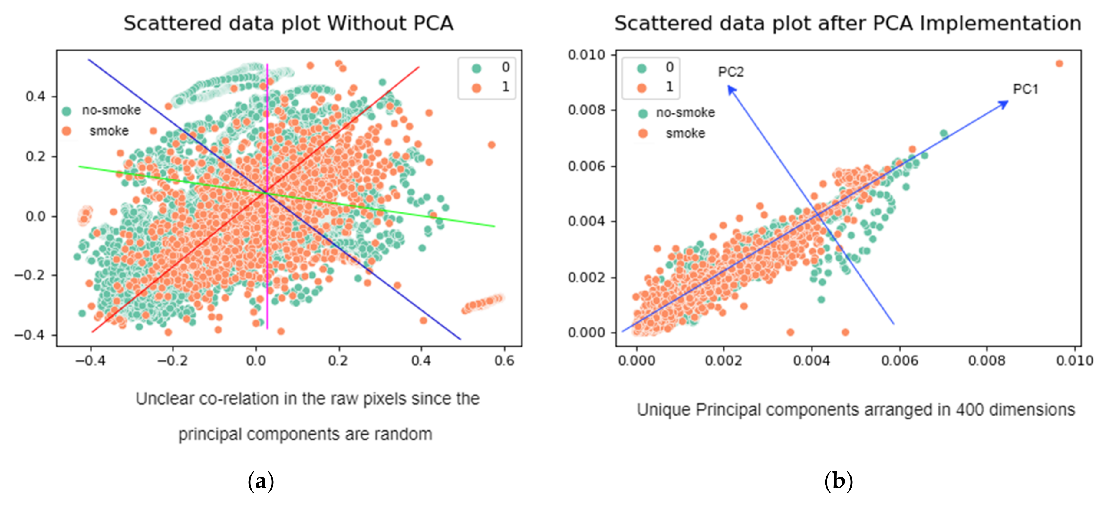
The principal component analysis serves as a visualization tool for the pixels of smoke and non-smoke instances as data points. PCA integrated with the improved YoloV3 as a pre-processing module. Instead of using raw pixels of images data, we projected our data into PCA space to transform it into a lower-dimensional space. In Figure 4a, the scatter plot “a” represents raw pixels in multidimensional space. The scatter plot “b” shows PCA transformed variables (pixels). 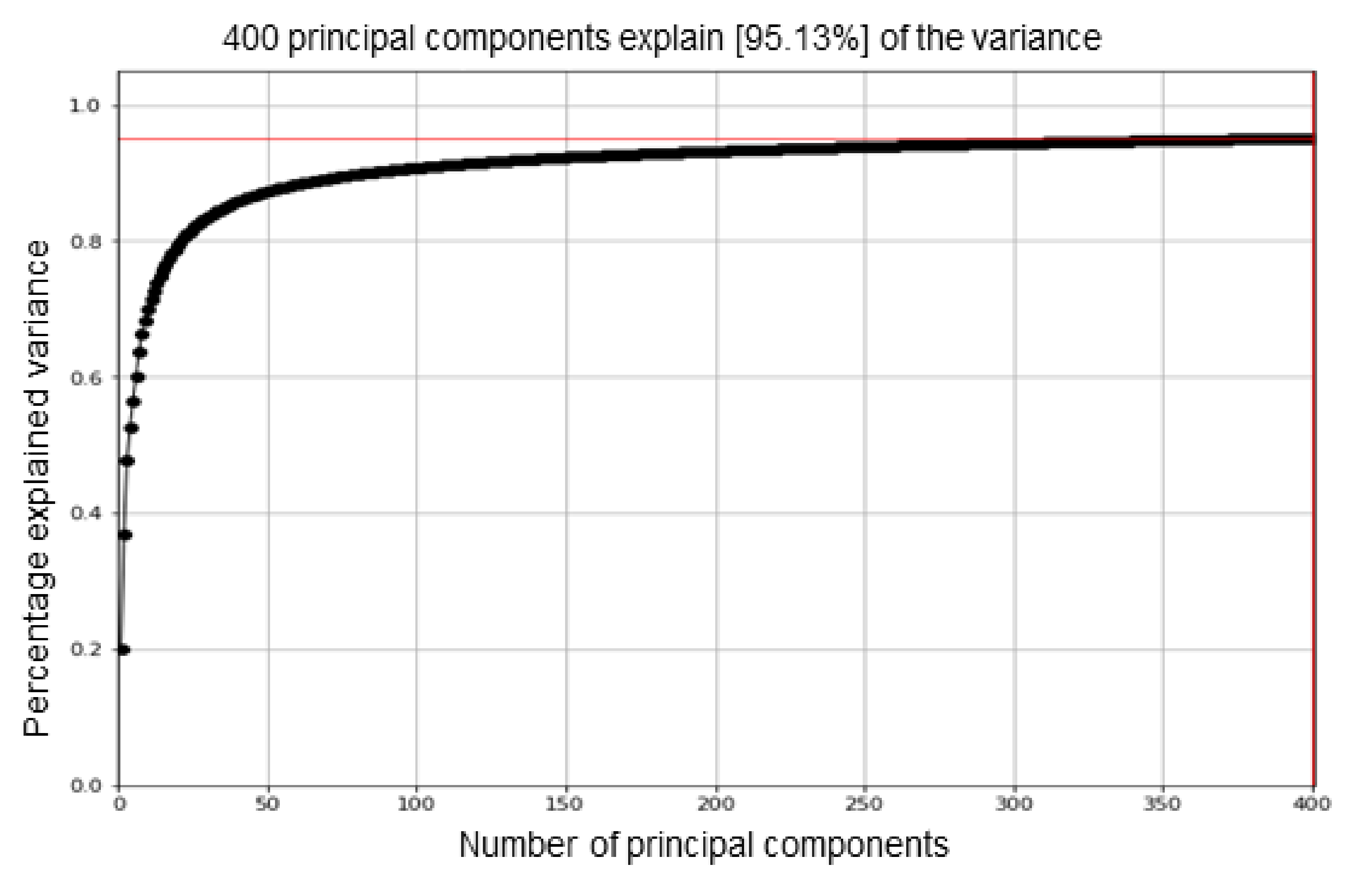In Figure 4b, total pixels are less in numbers than the raw pixels. It proves that PCA selects the important features discarding the redundant features. We have selected only 400 principal components showing only 400 dimensions of the features. The cumulative explained variance is almost 95%. It shows the effectiveness of the PCA module towards the input dataset.

Figure 4. Scatter graphs (a,b) represent the random and unique dimensions of smoke and non-smoke pixels. In plot (b), the total number of scattered pixels decreases because PCA selects the most co-related pixels. The principal components represent the directions of each pixel. Those components describe the total percentage of explained variance.

We have 9347 smoke and 4453 non-smoke 2D images. Each image is of resolution 416 × 416. The total dimensions of our dataset are 13,800 × 416 × 416. The size of the data matrix is [$H$]_{13,800 × 416 × 416,} thus the sizes of covariance matrix $C$ and transformation matric $M$ are the same. This huge dimensional space increases latency in the training and testing of the detector. To reduce the random dimensions of raw pixels, PCA selects the minimum number of principal components with respect to the percentage of explained variance.

Figure 5 shows the selection of independent components. The cumulative explained variance selects the number of components. A total of 400 principal components reduce the dimensions of dataset variables as 13,800 × 400 and the cumulative explained variance is 95.13%.

Figure 5. The graph represents the number of principal components and cumulative explained variance. The rising curve shows the selection of only 400 principal components describes approximately 95% variance. PCA selects 400 principal components without losing much information.

3.5. Experimental Settings

This section explains the specific details of datasets and test train split for experimentation. In addition, it explains the hyper-parameters setting and working environment.

3.5.1. Dataset Description

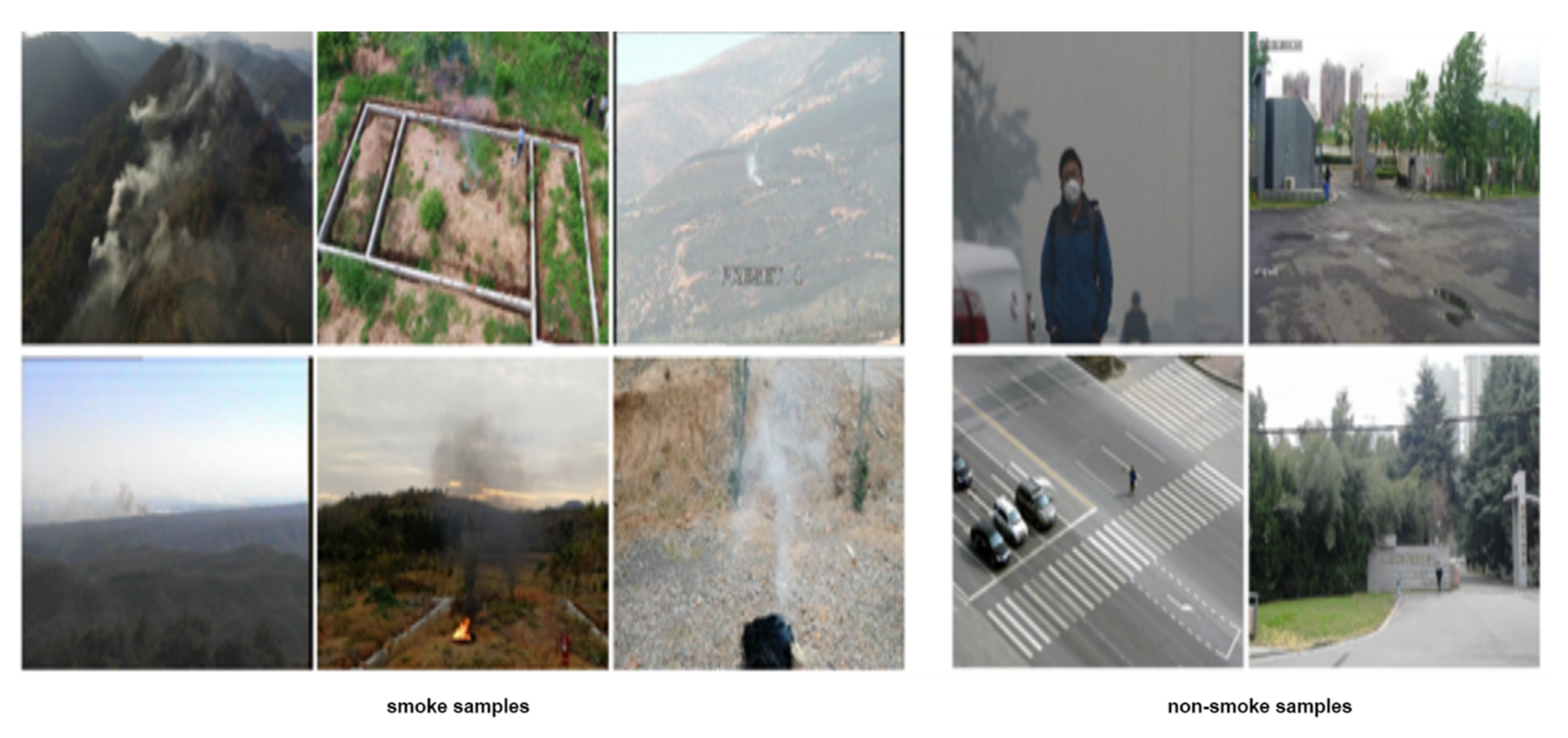
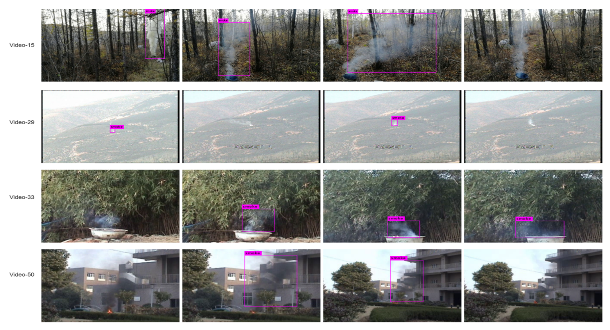
The datasets contain 9347 smoke images extracted from high-definition videos. The database also includes 4453 still images of non-smoke instances resembling smoke. Extra small smoke instances are captured in the wild with mountains in the background with various weather conditions i.e., in a fog, illuminations, and moving clouds. The camera sensor mounted on the unmanned aerial vehicles (UAV) captures those smoke instances in the surroundings of Huangshan, China.

Figure 6 represents some samples of smoke and non-smoke from the original database.

Figure 6. A view of smoke samples. Smoke instances are extra small and of less density with a challenging background. Non-smoke images are also challenging with moving trees, cars, and persons.

3.5.2. Training & Testing Division

The original database is divided into two sets, i.e., the trainval set, and the test set. A test set accommodates 20% (or 2760) smoke and non-smoke instances out of 13,800 total images. All the remaining 80% images are in a trainval set. From a trainval set, the network automatically uses the next batch of a train set as a validation set. The trainval set serves as training images and validation images. The validation set ensures the monitoring of the network convergence and overfitting.

3.5.3. Hyper-Parameters Setting

The training parameters for the traditional and improved YOLOv3 are as follows:

We select the learning rate as 0.001 at the beginning of the training. The batch size of the network training is 64, and the momentum decay is 0.9. We use stochastic gradient descent (SGD) as an optimizer as it can optimize the network conveniently, i.e., converge the network faster as compared to Adam.

One forward pass and backward pass makes two iterations and one epoch. In our experiments, the total number of iterations is different for both networks. We marked all images in PASCAL VOC format by an open-source labeling tool LabelImg to tag all images as XML files.

3.5.4. Working Environment

All experiments are conducted under the experimental environment using deep learning open source framework Darknet, the operating system Ubuntu 16.04, Machine learning library TensorFlow, CPU Intel Core i7-6850K CPU @ 3.60 GHz (×12), GPU (×3).

4. Experimental Results & Discussion

This section explains the evaluation criteria and the comparison of results from traditional and improved networks. A brief discussion presents the metrics calculation methods and their high-level comparison.

4.1. Training Metrics Evaluation

Figure 7 and Figure 8 represents the loss curves for ordinary YOLOv3 and improved YOLOv3 with the number of iterations. Both detectors trained on different numbers of iterations. The reason is that the training iterations are not manually selected. The network terminates the training procedure when the network observes the best weight with minimum loss and maximum validation accuracy. Hence, in the case of ordinary YOLOv3 after 4000 iterations, there is no regular increase in validation mAP and no significant decrease in average loss. Therefore, ordinary YOLOv3 early stops the training after 4000 iterations. The tuned version of YOLOv3 terminates the training process after 8000 iterations.

Figure 7. Represents the relation between average training loss and validation accuracy as mean average precision (mAP) for traditional YOLOv3. The training loss decreases consistently with increase in number of iterations. The mAP for validation sets increases in the same trend.

Figure 8. Represents the relation between average training loss and validation accuracy as mean average precision (mAP) for four scales YOLOv3-PCA network. The training loss decreases consistently with an increase in the number of iterations. It shows that the loss is less than ordinary YOLOv3 and the mAP of a validation set for improved YOLOv3 is 94% which is greater than ordinary YoloV3.

Test Metrics Analysis

The necessary result metrics to calculate and evaluate the detection accuracy and sensitivity of the trained models are average precision (AP) or mean average precision (mAP) and F1-scores. The area under the PR curve calculates the AP metric. The precision and recall rates determine the F1-score to evaluate the trained model. Figure 9 draws the PR curves for ordinary YOLOv3 and improved YOLOv3.

Figure 9. The area under PR curves for traditional model and improved YOLOv3 shows average precision at specific recall. The black curve covers more area that represents greater AP & mAP for improved version of YOLOv3.

We have used 11 points method to draw PR curves for both models. We can see the area under the curve for improved YOLOv3-PCA is greater than the traditional YOLOv3. The endpoint of PR-curve in the case of an improved model is at a higher precision value. Therefore, due to the more precision rate of the improved model, its PR-curve covers more area. As a result, its average precision is more than the traditional model. The AP for an improved model is 95.60%, and the AP for a traditional YOLOv3 is 94.01%.

The total number of true positives (TP), false positives (FP), and false negatives (FN) compute the precision rate and recall rate. True positives and false positives are responsible for the precision rate. True positives and false negatives are responsible for the recall rate of the detectors. F1-score of the model determines its overall efficiency showing the accuracy for foreground object and sensitivity of the model for background object. Intersection over Union (IoU) threshold and probability threshold decides the values of test metrics. The total number of correctly detected samples and the total detected samples changes with the change in the two threshold values. In conclusion, the variation in probability threshold changes the precision rate and recall rate. The IoU threshold brings variation in the AP and mean average precision (mAP) metrics. Hence, 11 values of precision and recall draw PR curves for both models. For a best_weights of ordinary YOLOv3 and improved YOLOv3, we calculate their respective recall and precision rates at 11-probability threshold values keeping IoU = 0.35, Table 1 and Table 2. Our experiments also calculate the mean average precision (mAP) for both detectors. The mean of AP values at five IoU thresholds, i.e., {IoU = 0.3, 0.35, 0.4, 0.45, 0.5} gives mAP while keeping the probability threshold fixed at 0.35. Table 1 and Table 2 shows the test metrics at different probability thresholds.

Table 1. Test metrics for improved YOLOv3-PCA model at different values of probability threshold while keeping intersection over union constant at IoU = 0.35.

Network	AP%	Precision(P)	Recall(R)	F1	Probability Threshold
YOLO-PCA	95.60	0.90	0.91	0.91	0.1
		0.95	0.83	0.89	0.2
		0.96	0.79	0.87	0.25
		0.97	0.75	0.85	0.3
		0.98	0.73	0.83	0.35
		0.98	0.68	0.81	0.4
		0.99	0.60	0.75	0.5
		0.99	0.52	0.68	0.6
		0.99	0.43	0.60	0.7
		1.00	0.34	0.50	0.8
		1.00	0.23	0.38	0.9

Table 2. Test metrics for traditional YOLOv3 model evaluated at 11- probability threshold values while keeping IoU = 0.35.

Network	AP%	Precision(P)	Recall(R)	F1	Probability Threshold
Traditional YOLOv3	94.01	0.78	0.93	0.85	0.1
		0.90	0.87	0.88	0.2
		0.93	0.82	0.87	0.25
		0.94	0.77	0.85	0.3
		0.95	0.73	0.82	0.35
		0.97	0.68	0.80	0.4
		0.98	0.57	0.72	0.5
		0.98	0.46	0.63	0.6
		0.99	0.35	0.52	0.7
		1.00	0.26	0.41	0.8
		1.00	0.16	0.27	0.9

4.2. Discussion

As the recall, precision, and F1-score, all these metrics vary with the number of true positives, false positives, and false negatives. The following formulas calculate the precision rate, recall rate, and F1-score.

$$P=\frac{TP}{TP+FP}$$

(5)

$$R=\frac{TP}{TP+FN}$$

(6)

$$F1=2\times \frac{TP}{TP+FP}$$

(7)

• $TP$ = When there is smoke and it detects as smoke
• $FP$ = When there is no smoke and it detects as smoke
• $FN$ = When there is smoke and it detects as no smoke

The constant IoU threshold affects both precision and recall. We can see in Table 1 and Table 2, when precision increases with an increase in probability threshold, recall decreases. It is precision that decides the area under the PR curve. It means the precision rate directly affects the AP.

In simple words, precision means the quality of the results, and recall shows the quantity of relevant or irrelevant results. At a high probability threshold, the quality improves i.e., precision improves because only the most relevant results are retrieved while discarding the others.

We compare the ordinary YOLOv3 and improved YOLOv3-PCA models in high-level percentages instead of percentage points. Because, at 11-points of the probability threshold, we calculate the precision and recall rates. Therefore, we can compare both models in high-level percentages by computing the average of all precision rates, recall rates, and F1-scores. After calculating the average of all metrics, it is possible to determine the high-level percentages of precision, recall, mean harmonic, average precision (AP), and mean average precision (mAP) by the following formula.

$$MP=\frac{MIM-MOM}{MIM}\times 100$$

(8)

• $MP$ = metric percentage
• $MIM$ = mean of improved metric
• $MOM$ = mean of ordinary metric

The experimental results have improved with precision rate, recall rate, and mean harmonic (F1-score) by 2.67, 3.06, and 5.59 percentages. The respective improvements in average precision (AP) and mean average precision (mAP) are 1.66 and 2.78 percentages.

Table 3 shows the average (mean) of precision rate, recall rate, and F1 for improved YOLOv3-PCA and ordinary YOLOv3.

Table 3. The mean of improved metrics and ordinary metrics.

Networks	Mean(P)%	Mean(R)%	Mean(F1)%	IoU Threshold	Probability Threshold
Traditional YOLOv3	94.7	60.0	69.2	0.35	[0.1…0.9]
YOLOv3-PCA	97.3	61.9	73.3	0.35	[0.1…0.9]

The mean of AP values at different IoU calculates the mAP metric for both detectors. The mAP is the measure of the overall detection performance of a model. From Table 4, the mAP for an improved model is increased up to worth noting.

Table 4. Table shows the Average precision (AP) at different IoU thresholds. The mean of “AP” values gives mean average precision (mAP).

Networks	AP% IoU = 0.3	AP% IoU = 0.35	AP% IoU = 0.4	AP% IoU = 0.45	AP% IoU = 0.5	mAP%
Traditional YoloV3	94.01	93.06	91.69	89.30	85.16	90.64
YoloV3-PCA	95.60	94.67	93.65	92.26	90.04	93.24

Figure 10 shows the visual comparison for the testing of 3-scale YOLOv3 and 4-scale YOLOv3-PCA algorithms. Figure 10 illustrates the detected samples by improved YOLOv3-PCA network while out of them, the traditional YOLOv3 detects a few correctly. The reason is that in those samples the smoke instances are immensely small. Additionally, in some samples the smoke is very thin, i.e., appeared as low-density smoke.

Figure 10. The visual comparison for the testing of 3-scale YOLOv3 and 4-scale YOLOv3-PCA algorithms. Figure 10 illustrates the detected samples by improved YOLOv3-PCA network while out of them, the traditional YOLOv3 detects a few correctly.

We have presented the visual comparison for both detectors. We selected challenging smoke instances from test set and tested by the both detectors. The improved YOLOv3 detects all samples correctly while out of them traditional YOLOv3 detects a few correctly while the rest are missed.

Figure 11 represents missed detection by the improved YOLOv3-PCA model in successive frames in videos. Out of a few reasons for missed detection by the improved YOLOv3-PCA model is a severe atmospheric condition that may cause a sudden change in the shape of the smoke. Similarly, when the motion trajectory for smoke movement changes, the model changes its decision. The improved model may predict samples precisely if we add the motion vectors of smoke. In the future work, we will present a more generalized network where we will add motion features in the training phase of the network.

Figure 11. An improved model ignores a few smoke instances in successive frames in videos. Overall, Figure 11 shows a satisfactory performance of the extra-scale YOLOv3 model, also showing space for further improvements.

5. Conclusions

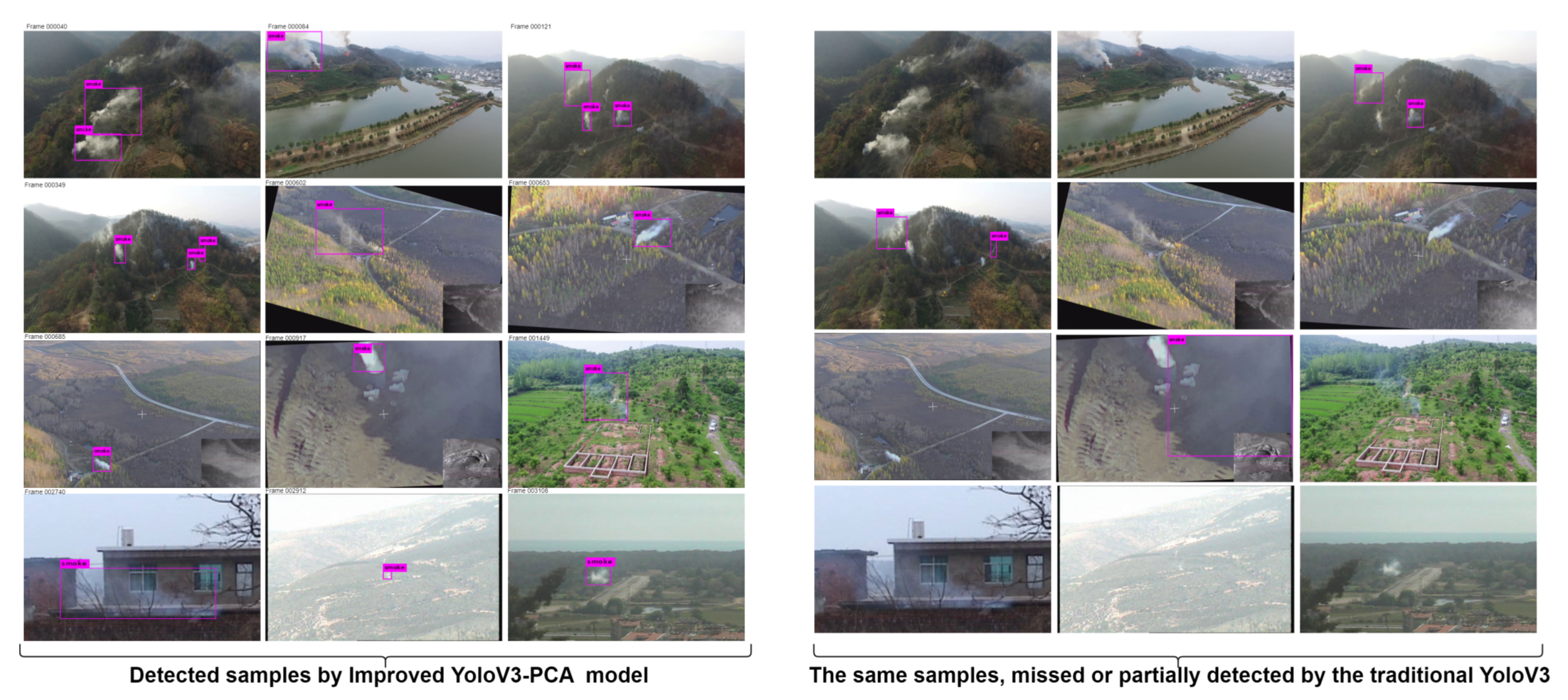
This paper integrates Principal Component Analysis as a simple data pre-processing module with an improved version of YOLOv3. The implementation purpose of the entire framework is to evaluate the detection results of immense small smoke instances in actual aerial images captured in the wild.

To boost up the network predictions for correct smoke labels and localization of smoke instances in the wild, we add an extra scale of detection in the actual structure of the traditional YOLOv3.

Principal component analysis pre-processes the raw datasets to extract the most useful features in less dimensional space. It discards the redundant features present as raw pixels in the original datasets. Additionally, it makes the visualization of results explicit.

The improved network evaluates our self-built datasets containing smoke images in challenging environments and non-smoke instances similar to smoke.

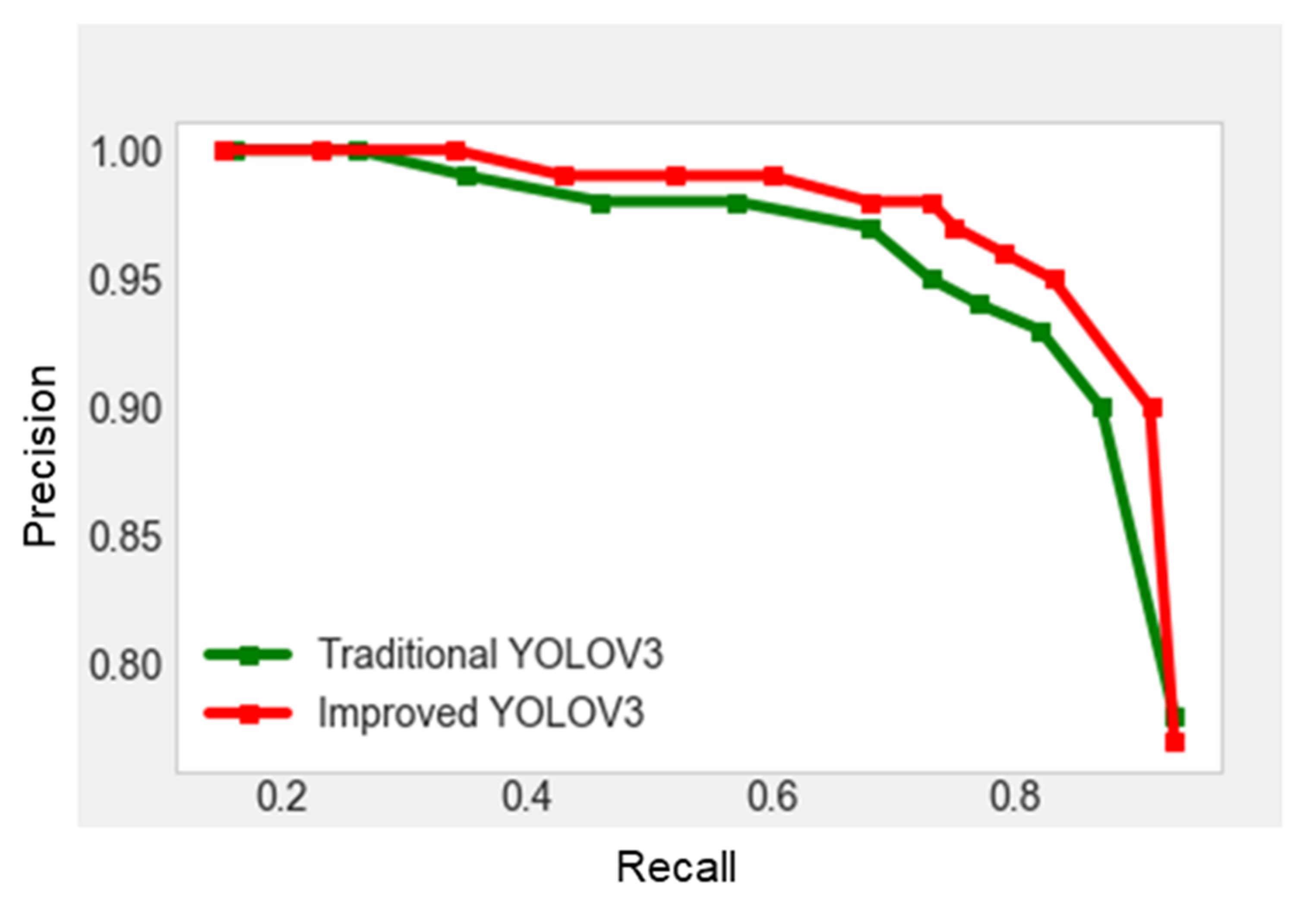
Our experiment reports a notable gain in mAP for improved YOLOv3-PCA combination. In addition, the other metrics such as precision and recall rates are also high. The hybrid scheme may prove to be of great interest for fire managers to detect forest fire on time and for firefighters to locate the exact position and growing nature of fire.