Article

Megafires in a Warming World: What Wildfire Risk Factors Led to California’s Largest Recorded Wildfire

1
Department of Geography, University of California Santa Barbara, Santa Barbara, CA 93106, USA
2
Earth Research Institute, University of California Santa Barbara, Santa Barbara, CA 93106, USA
3
Agriculture and Forestry Wildfire Management Branch, Edmonton, AB T6H 5T6, Canada
*
Author to whom correspondence should be addressed.
Submission received: 8 December 2021 / Revised: 20 January 2022 / Accepted: 21 January 2022 / Published: 25 January 2022
(This article belongs to the Special Issue Fire in California)

Abstract

:
Massive wildfires and extreme fire behavior are becoming more frequent across the western United States, creating a need to better understand how megafire behavior will evolve in our warming world. Here, the fire spread model Prometheus is used to simulate the initial explosive growth of the 2020 August Complex, which occurred in northern California (CA) mixed conifer forests. High temperatures, low relative humidity, and daytime southerly winds were all highly correlated with extreme rates of modeled spread. Fine fuels reached very dry levels, which accelerated simulation growth and heightened fire heat release (HR). Model sensitivity tests indicate that fire growth and HR are most sensitive to aridity and fuel moisture content. Despite the impressive early observed growth of the fire, shifting the simulation ignition to a very dry September 2020 heatwave predicted a >50% increase in growth and HR, as well as increased nighttime fire activity. Detailed model analyses of how extreme fire behavior develops can help fire personnel prepare for problematic ignitions.

1. Introduction

In 2020, wildland fires burned over 4 million acres in California (CA), the most recorded in a single year (Figure 1) [1]. A large portion of the burned area resulted from an anomalous dry lightning storm that struck in the middle of an August 2020 heatwave [2]. Fires ignited all over the central and northern portion of the state, later joining into a number of massive burns, referred to as complexes. Multiple fire behavior drivers aligned to make this fire siege unprecedented. The previous winter—CA’s wet season—had above average precipitation in December but then decreased in January through March, which caused overall below average precipitation in much of northern CA and the Sierra Nevada Mountains [3]. Low winter precipitation causes more flammable, rapidly drying fuels, which was evident in July 2020 by below average live fuel green-up and dead fuel moisture content. As warm, dry conditions persisted through July, the number of wildfires increased. Then, moisture advected from tropical storm Fausto, off the coast of Baja California, streamed northward, causing over 15,000 lightning strikes throughout central and northern CA [1].
Near the confluence of Tehama, Glenn, Mendocino, and Lake counties, thirty-seven individual fires ignited during the August siege. The Doe Fire quickly became the largest of those fires and is the focus of this study (Figure 1). It predominantly burned in the remote Mendocino National Forest, spreading through a mixture of fuels, including mixed conifer, shrubs, and grass. Fire management resource unavailability, due to the number of ongoing fires, kept fire suppression efforts initially reduced, despite threatening fire behavior [1]. As the Doe Fire merged with the other individual fires, they formed the August Complex, which burned over 404,685 ha (1,000,000 acres) by early October, the most ever recorded by a single fire event in CA. The uncontrollable nature of this megafire cost over $115 million and a firefighter’s life [2].
The fire regime of a region is defined by where and when wildfires occur, how they behave, and how they affect the landscape [4]. Research at scales ranging from individual fires to regional fire activity over multiple seasons has demonstrated that the mixed conifer forests of northwestern CA have a mixed-severity fire regime [5]. The highest severity fires are most often caused by extreme fire weather, including high temperatures and low atmospheric moisture [6,7]. Weather driven, high severity fires can also be intensified by complex topography and dry fuels, which was seen during the Doe Fire. On a larger scale, increases in extreme fire behavior throughout CA and the western United States (USA) have been attributed to atmospheric warming and drying caused by climate change [8,9,10,11,12,13]. A warmer atmosphere causes an increase in vapor pressure deficit (VPD) because saturation vapor pressure exponentially increases with temperature [10]. VPD increases cause decreases in fuel moisture content [14]. As climate change continues, heatwave frequency and intensity are also increasing in CA [15,16,17,18]. Changing precipitation patterns present the possibility of increased drought frequency [19] and a longer, drier fire season [20,21]. With extreme weather becoming more likely, it is critical to ask the following question: How will megafire behavior change with increased warming of the planet?
This study aims to contribute to this investigation by employing wildfire model simulations of the first four days of the Doe Fire, the largest individual fire that contributed to the August Complex. Specifically, we investigate the following three questions: (1) What meteorological variables (winds, relative humidity (RH), temperature) and fuel conditions contributed most to the rate of fire spread? (2) How would the Doe Fire have evolved if the ignition had occurred during a second, stronger heat wave observed in September 2020? (3) How do fire characteristics (area burned and heat release) vary with changes in temperature and aridity? To answer these three questions, we used the Canadian fire spread model Prometheus [22]. This choice was based on the model’s widespread use [23], simplicity, contemporary updates, and the availability of Canadian fire danger indices in the global reanalysis used in this study. In preliminary work, Prometheus also outperformed USA-based models FARSITE and FlamMap, which prompted an attempt to test its capabilities in CA.
Section 2 of this paper describes the model calibration and experimental design. Section 3 discusses our findings. The results of the control model run of the Doe Fire, including fuel consumption, rate of spread (ROS), and fire heat release (HR) analyses are presented and discussed in Section 3.1. Next, we discuss model sensitivity tests to several meteorological inputs, FMC scenarios, and ignition time tests in Section 3.2, Section 3.3 and Section 3.4. Section 3.5 then describes the connection between warming/drying and fire spread. Section 4 contains our concluding remarks. An acronym table is included in Appendix A (Table A1).

2. Materials and Methods
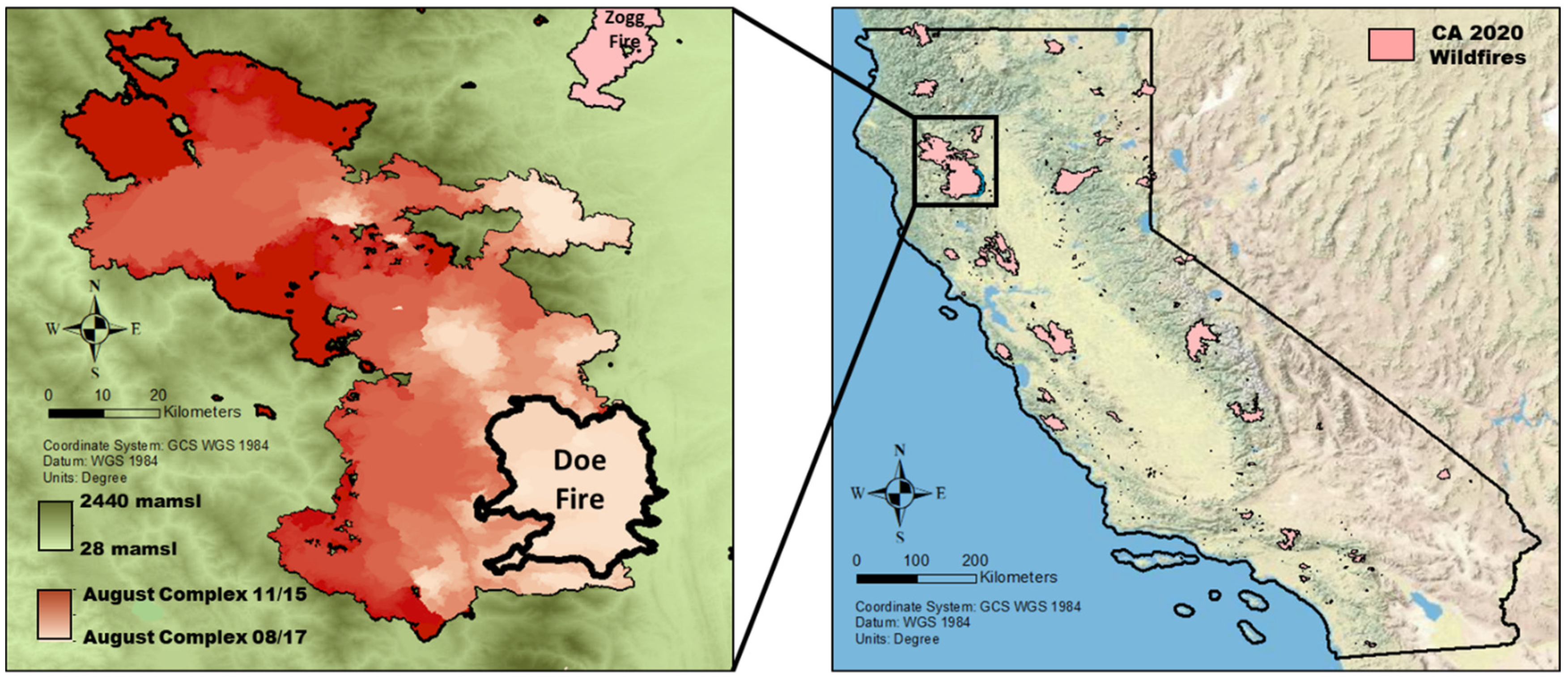
2.1. Case Study

We simulated the Doe Fire because it was the largest individual contributor to CA’s largest recorded wildfire—the August Complex. The initial growth was also minimally influenced by suppression actions, which are difficult to account for in fire spread modeling. The Doe Fire began on 16 and 17 August from at least three different lightning strikes—detected by analyzing NASA’s Visible Infrared Imaging Radiometer Suite (VIIRS) fire detection data. On 18 August, its perimeter was reported as 566 ha. Then, hot, dry weather and gusty winds caused the fire area to explode to 52,280 ha by 22 August. Fire behavior lessened after 22 August, which motivated us to simulate the four days of extreme behavior between 18–22 August. In Prometheus, we set the ignition time to 1200 Pacific Daylight Time (PDT) on 18 August, rather than 16 or 17 August, because Prometheus was not able to capture the initial post lightning strike or slow evolution of fire growth. We then ran the simulation for 96 h. Daily shapefiles of observed fire progression during August and September 2020 were obtained from FireNet (https://www.firenet.gov/, accessed on 23 September 2020).

2.2. Fire Model

Prometheus, the Canadian wildland fire growth simulation model, uses a deterministic approach to simulate the spread of wildfire with wave propagation equations and the Canadian Forest Fire Behavior Prediction System [24]. The fire is represented by a growing polygon, and at every model time step, the vertices of that polygon serve as points where new fire ellipses grow. After every time step, a new perimeter is drawn by tracing a tangential line around all of the new fire ellipses. The nature of the wave propagation technique produces outputs along each time step perimeter, but Prometheus also includes built in interpolation methods—inverse distance weighting, Voronoi area weighting, and nearest vertex—for gridded fire behavior outputs [22]. The spread of each ellipse and associated outputs are based on Canadian Forest Fire Behavior Prediction System equations. An initial ROS value is determined using the fuel type, wind speed, and fuel moisture content (FMC) of fine fuels. That ROS value is then recomputed using a net effective wind speed, which accounts for slope. The net effective wind direction also accounts for slope and determines the fire spread direction. ROS can be further affected by a buildup effect, which factors in larger combustible fuel availability using longer time lag FMC indices. Crown fire behavior, which can also increase ROS, occurs when a critical surface fire intensity is reached, which depends on a fuel type’s crown base height and foliar moisture content. Crowning also affects the total fuel consumption, calculated by adding surface fuel consumption—based on fuel moisture and availability—and crown fuel consumption—based on crown fraction burned and fuel load. The associated equations are based on fire observations or best judgement when observations were not available [24,25]. The Forest Behavior Prediction System and Prometheus do have some limitations. Short-range spotting is accounted for within the ROS equations, but long-range spotting is not accounted for, although Prometheus does allow the fire to breach a barrier that is at most 1.5 times the flame length. Due to its two-dimensional nature, Prometheus does not account for interactions between merging fires and between fires and the atmosphere [22], both of which occurred during the Doe Fire [26]. These limitations reduce the accuracy of output values, but analysis of and comparisons between simulations are still helpful in understanding extreme fire behavior.

2.3. Meteorological Inputs

Meteorological data (wind speed/direction, temperature, RH, and precipitation) can be input as either hourly point streams, grids, or daily values. We chose to use hourly streams because Prometheus also has an option to spatially interpolate meteorological variables across the domain using multiple points [22]. This method allowed us to use four locations from ERA5 reanalysis [27] as “virtual weather stations”, the coordinates of which are 39.5° N, 122.5° W; 39.5° N, 122.75° W; 39.75° N, 122.5° W; and 39.75° N, 122.75° W. These locations surround the Doe Fire perimeter (Figure 2). To assess the feasibility of using the coarse resolution ERA5 reanalysis for the weather locations, we also ran a test simulation using six virtual weather stations from a Weather Research and Forecasting (WRF) model downscaling run. The modeled fire behavior was similar when comparing the higher resolution (2 km) WRF meteorological inputs to the coarser (0.25°) ERA5 inputs. We therefore chose to use ERA5, alleviating computational intensity and making it easier to investigate several scenarios. Prometheus requires the selection of a primary weather stream. We chose the northwest location because it fell within the perimeter of the Doe Fire and was at a representative elevation.

2.4. Topography and Fuel Inputs

A digital elevation model (DEM) and fire behavior fuel model—LF 2016 Remap Scott/Burgan 40—for the Doe Fire region were obtained through the LANDFIRE Program [28]. The LANDFIRE data were converted from the default raster format to gridded ASCII files. We also upscaled the elevation and fuel inputs from a 30 m resolution to a 300 m resolution, which later allowed us to increase simulation temporal length and resolution. Prometheus cannot directly import USA-based fuel models, so we created a fuel lookup table (Table A2) comparing the USA Scott/Burgan fuel model and the Canadian fuel types that are built into the model. We matched USA fuel model ROS curves [29] for each fuel in our domain with Canadian ROS curves [24]. Fuel loads were not compared, which reduces the accuracy of fuel consumption and intensity outputs. The Canadian mixedwood fuel type was primarily used in the fuel lookup table because the ROS can be adjusted by changing the ratio of conifer to deciduous composition. The Canadian fuel types also do not include any shrub fuels, which limited the options for converting USA-based shrub fuels. Example fuel descriptions, ROS curves, and conversion charts are provided in Table A3 and Figure A1.
Prometheus also requires FMC inputs from the day before simulation start time. These include the fine fuel moisture code, duff moisture code, and drought code. The fine fuel moisture code ranges from 0–101 and indicates the FMC of forest litter fuels; the duff moisture code represents the moisture content of organic material under the litter; and the drought code indicates the moisture conditions of deep soil drying similar to the Keetch–Byram Drought Index, and can be indicative of vegetation drought stress [30]. Daily FMC indices are available through ERA5 reanalysis. Higher values correspond to drier fuels.

2.5. Model Calibration

Prometheus includes an option to stop fire spread when certain burning conditions—initial spread index, fire weather index, wind speed, and RH—are not met. For additional details on initial spread index and fire weather index descriptions and calculations, refer to [24]. We modified the model default burning conditions until our simulation accurately reproduced the observed fire growth (Table 1). The default values were embedded in Prometheus but not discussed in the model reference [22]. We also noticed model predictions of errant fire spread into the Sacramento Valley to the east. The Doe Fire did not spread there because of suppression efforts, sparser fuels, and less complex topography [31]. To reproduce the observed fire behavior, we created a fuel patch that designated all dry climate grass (GR2) fuels in that area as non-burnable. A band of north–south running dry climate grass-shrub (GS2) and dry climate shrub (SH7) was also showing excessive fire spread to the north. In our fuel lookup table (Table A2), these correspond to Canadian mixedwood fuel types because the Canadian fuel model does not include shrub fuels. The mixedwood fuel type allows for adjustment of the ratio of deciduous to conifer. We lowered the conifer percentage, which lowers ROS, of both the dry climate grass-shrub—originally 70 percent—and dry climate shrub—originally 85 percent—to 50 percent. These modifications were necessary due to the inherent differences between Canadian and USA fuels. Additional case studies could be helpful for creating a fuel lookup table that is practical for all CA biomes, beyond our study region. Finally, based on sensitivity tests, we used two centrally-located ignitions rather than the hypothesized 3+ ignitions due to the model emergent spread behavior (Figure 2). By combining these modifications with the required burning conditions, we were able to create a reasonable approximation of the fire footprint after four days of explosive Doe Fire growth, with daily comparisons presented later. This approximation allowed us to perform additional experiments to understand the factors underlying extreme fire spread behavior.

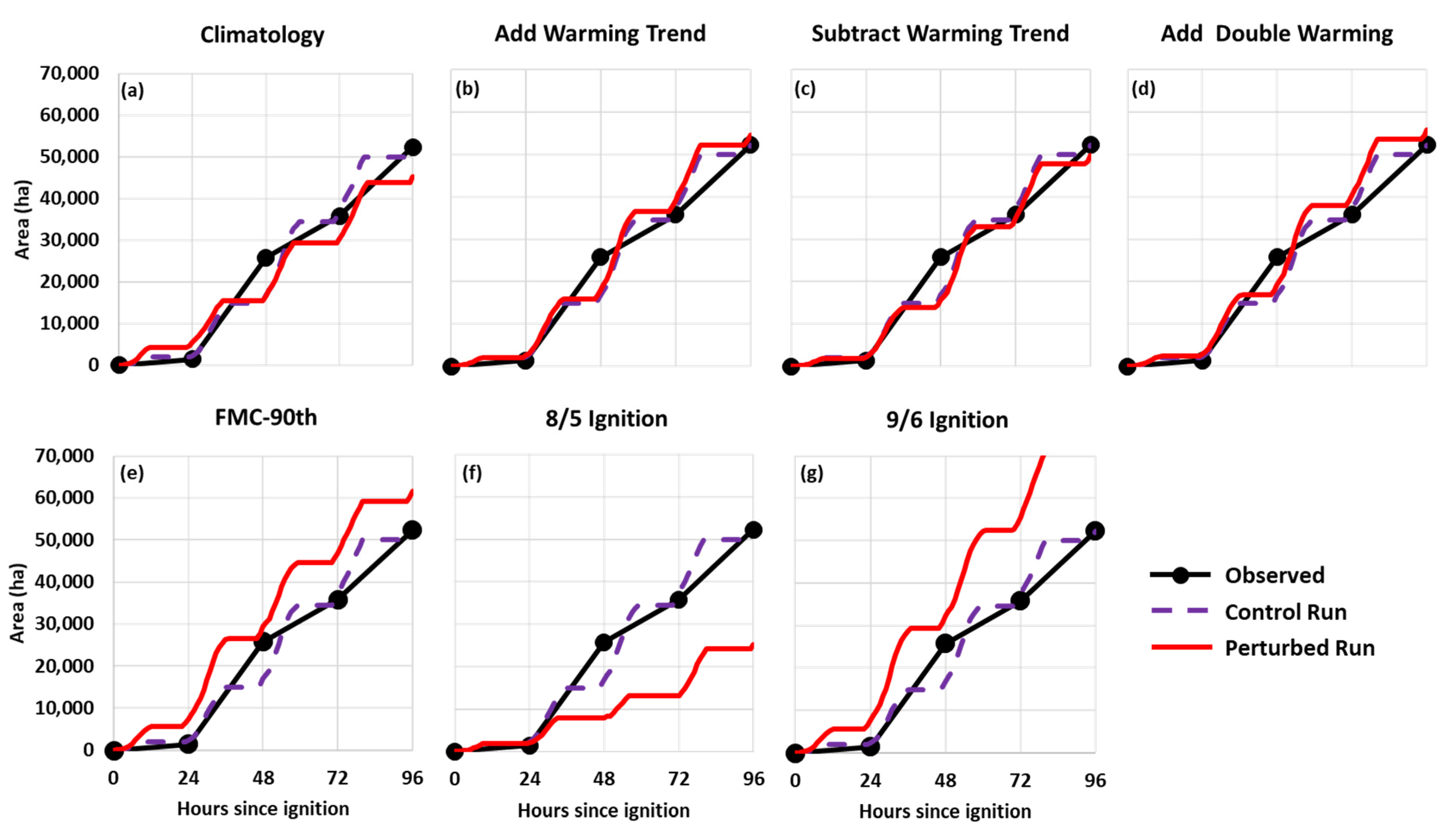
2.6. Experimental Design

We performed principal component analysis to determine the covariance and main modes of diurnal variability among the hourly meteorological inputs and fire behavior outputs. Additional details on principal component analysis methodology can be found in [32]. After testing different combinations of meteorological and fire behavior variables, we included 96 h long time series of temperature, RH, zonal and meridional winds, and ROS. We used the northwest ERA5 location (Figure 2) for our meteorological inputs because it is the primary weather stream, the most proximate to ignitions, and the closest to average domain elevation. The ROS time series is a sum of all gridded values over each time step.
Our additional simulation experimental design included seven different variations to the calibrated control run and was categorized as follows.

2.6.1. Sensitivity to Climate

In the first scenario, all hourly meteorological variables (wind speed/direction, temperature, RH, and precipitation) in each of the four weather streams were replaced by hourly climatological values. The 18–22 August climatology weather streams were derived by averaging each hourly value from 41 years (1979–2020) of ERA5 reanalysis data for each weather stream location (Figure 2). The 41-year averaged initial FMC values were also used for each weather stream. This scenario represents how the simulated Doe Fire behaves in mean weather conditions, i.e., no heatwave.
In the second and third scenarios, only temperature was perturbed by adding and subtracting increments of 0.8 °C from the original weather stream values. A trend of +0.8 °C warming was derived from a linear fit to the ERA5 reanalysis locations and estimated as the long-term (41-year) temperature increase in the region during August. We did not perturb the other meteorological variables during these simulations (wind speed/direction, RH, precipitation) because no statistically significant long-term trends were calculated, although this does not mean they will not change in the future. By subtracting 0.8 °C, we are simulating fire behavior during similar heatwave conditions before the recent 41-year warming trend, while adding 0.8 °C shows how modeled fire behavior could change in a future warmer world. In the fourth scenario, an increment of 1.6 °C was added to the control weather streams to further test the sensitivity to warming. The results of these temperature change scenarios prompted us to do additional temperature sensitivity tests, adding 0.4, 1.2, 2.0, and 2.4 °C to the control weather streams. These additional scenarios were used to illustrate the effect of warming on modeled fire growth.

2.6.2. Sensitivity to FMC

FMC variations were examined by computing the 41-year (1979–2020), 90th, 95th, and 99th percentile values of FMC indices (fine fuel moisture code, duff moisture code, and drought code) on 17 August at each of the four weather stream locations. These values were then input as the weather stream initial FMC conditions to represent Doe Fire ignition under more severe drought/fuel drying. All other model inputs were kept constant. Similar results were found with all three percentile values, so we only included the 90th percentile results.

2.6.3. Sensitivity to Heatwaves

In the first scenario, the time of ignition was changed to 5 August at 1200 PDT, which was before the 18 August heatwave, while in the second scenario, the ignition was set to 6 September at 1200 PDT, during a hotter, drier heatwave. During the 96 h simulations, mean temperature and RH values were as follows: August 5 was 24.7 °C and 37.7% RH, 18 August was 25.3 °C and 28.5% RH, and 6 September was 25.9 °C and 16.6% RH. We decided to use the control run winds instead of the observed winds during the altered ignition timing, so we could better determine the effects of temperature and aridity. These scenarios are used to investigate what would have happened to the Doe Fire had it ignited during different environmental conditions.
For every simulated scenario, fire area was compared to the observed growth and HR outputs were compared to the model control run. HR was chosen as an output because it influences suppression difficulty and fire effects. Calculated HR values are based on Canadian fuel type consumption, which reduces the accuracy, but comparisons between the scenarios are still relevant. To calculate HR, we multiplied the total fuel consumption (TFC) for each hour by a generalized heat-of-combustion constant [33]:
H R   k W = H e a t   o f   C o m b u s t i o n   k J k g * T F C   k g m 2 * C e l l   R e s o l u t i o n   m 2 T i m e   D u r a t i o n   s e c o n d s
Heat of Combustion = 18,000 kJ/kg

3. Results

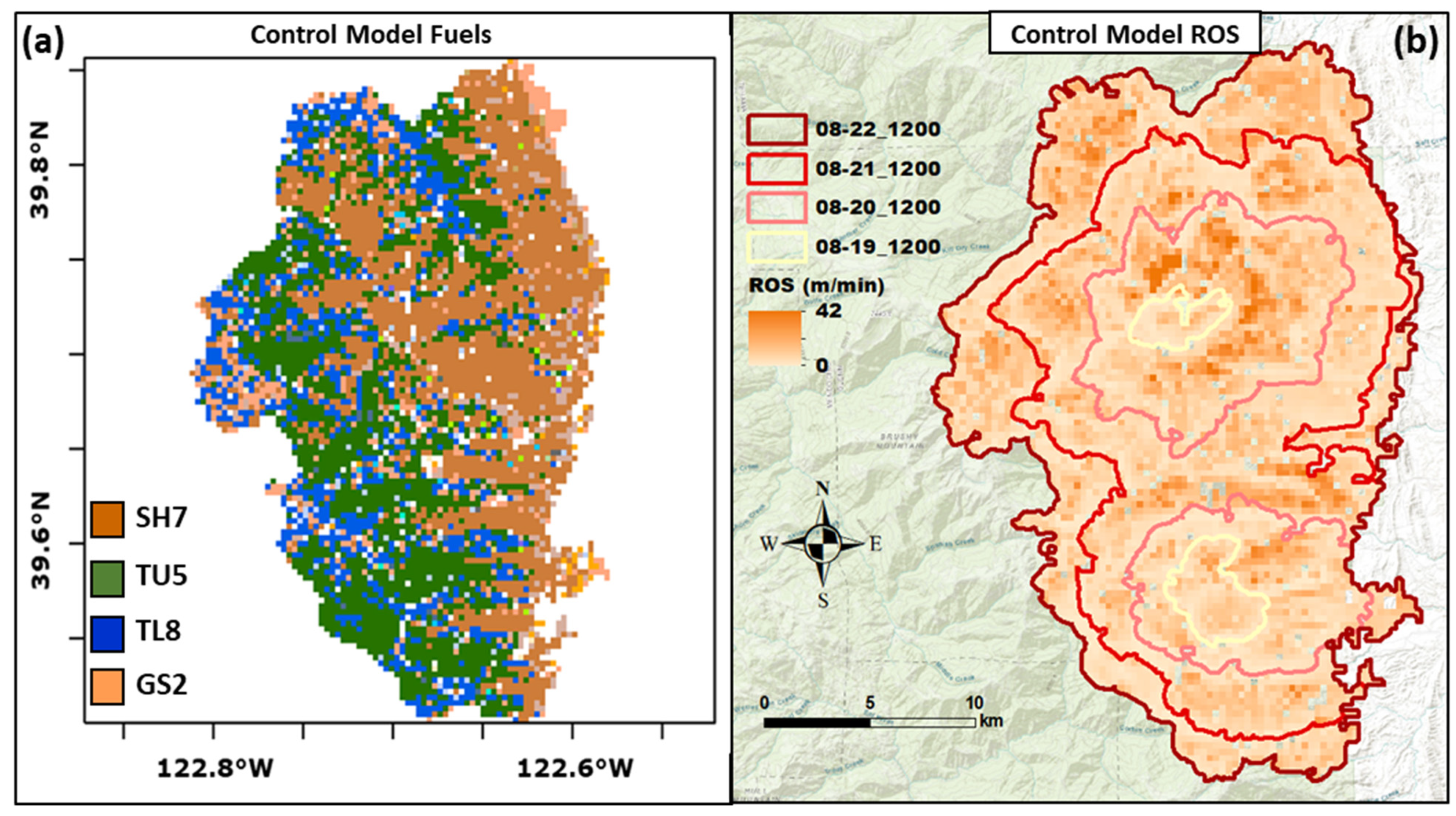
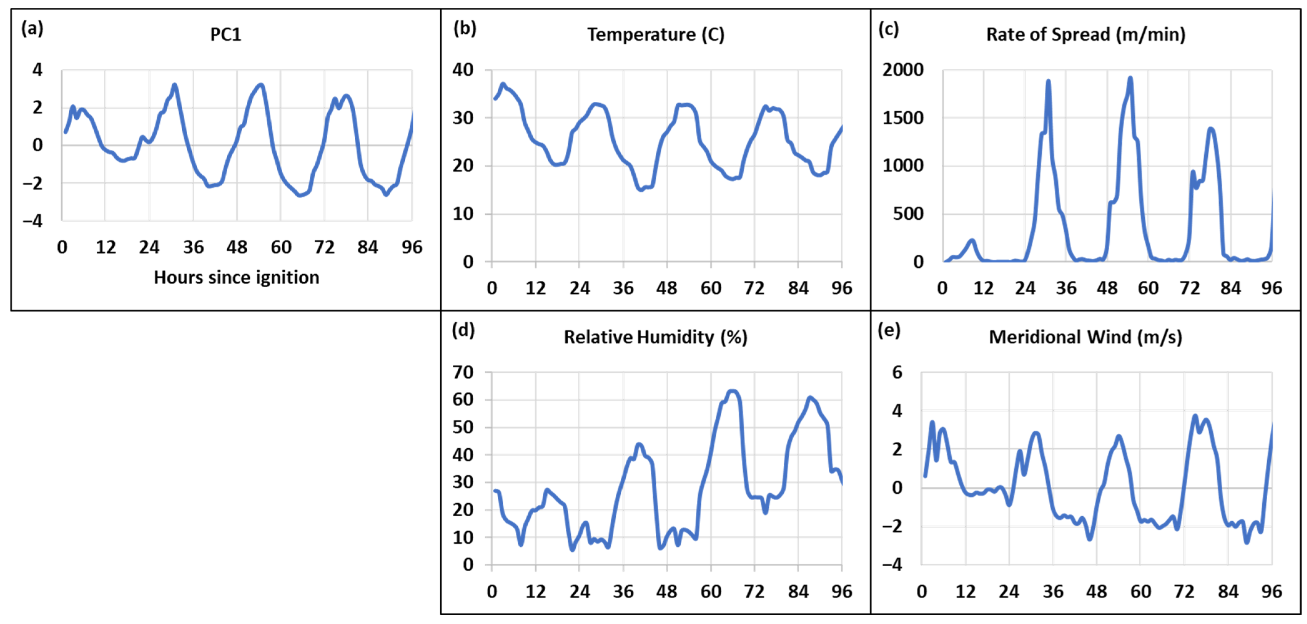
3.1. Control Run Simulation

The calibrated control run resulted in a four-day burned area of 52,245 ha, which is comparable to the observed Doe Fire size on 22 August: 52,281 ha (Figure 2). The simulated fire stopped spreading for 10–12 h each night and early morning because one or more of the burning condition thresholds were not met during that hourly time step, i.e., the wind speed/initial spread index/fire weather index was too low or the RH was too high. Reduced nighttime activity is typical wildfire behavior, although this is currently changing with increased warming and drying at night [34,35,36]. The fuels and ignition alterations also helped the shape of the control perimeter match with the observed perimeter, as seen in Figure 2. Within the control perimeter, the four dominant USA Scott/Burgan fuel models were as follows (Figure 3):
  • Very high load, dry climate shrub (SH7)—18,676 ha;
  • Very high load, dry climate timber-shrub (TU5)—15,244 ha;
  • Long-needle litter (TL8)—8095 ha;
  • Moderate load, dry climate grass-shrub (GS2)—3752 ha.
Figure 3 also shows the gridded ROS (m/min) experienced during the growth of the control run. The regions where modeled ROS was greatest occurred on 19 August and 20 August. Meteorological factors leading to temporal ROS differences were investigated through principal component analysis.
Figure 4 and Table 2 show the results of our principal component analysis, which helped test the sensitivity between the weather inputs and modeled fire behavior. The first eigenvalue of 2.94 explains 59% of the variance between temperature, RH, zonal/meridional winds, and simulated ROS. Temperature, meridional wind, and ROS were positively correlated to PC1, and RH was negatively correlated. These results indicate that high temperatures, a dry atmosphere, and daytime southerly winds were all closely linked to periods of high modeled ROS. None of these weather variables were the most extreme on record during this time period, especially wind speeds; however, the Doe Fire’s observed behavior was extreme, growing an average of 16,953 ha per day from 19–22 August.
When analyzing each burning day of the control—defined here as 1200–2200—we noticed important changes among averaged meteorological, fuel moisture, and modeled fire behavior variables (Table 3). During the first day, temperature was the highest, which coincided with the highest VPD, even with day 1 RH not being lowest. Mean ROS was the lowest on the first day, and mean HR was the second lowest. The highest VPD on day 1 preceded a drier FMC through days 1–3. Modeled ROS then peaked on day 2, followed by the highest HR on day 3. As the VPD decreased and RH increased, the fine fuel moisture code lessened on day 4, which corresponded to decreasing ROS and HR, despite consistently high temperatures.

3.2. Sensitivity to Climate

When we used 41-year climatologically averaged weather streams, the perturbed model run showed the fire initially spreading faster (Figure 5a) and producing more heat than the control (Figure 6a), due to higher winds on day 1 of the climatology. In days 2–4, the hotter and drier control run surpassed the climatology in both modeled area and HR. The climatology run eventually resulted in a −13.6% change in total area when compared to the observed perimeter and a −18.8% lower mean HR than the control (Figure 7). These differences indicate how sensitive fire growth predictions are to initial model conditions. Wind speed can drive greater ROS and HR, but winds are often more variable than temperature and RH, which influence larger spatiotemporal scale fire behavior.
Our next set of simulations involved perturbing temperature. Adding 0.8 °C (“Add Warming Trend”) caused steady increases in both area and HR throughout the simulation (Figure 5b and Figure 6b), resulting in a final area increase of 4.3% and a mean HR increase of 3.7% (Figure 7). When we doubled that warming trend (1.6 °C), the model showed a higher fire growth and HR increases during the four days Figure 5d and Figure 6d), ending with a 6.8% increase in area and a 6.2% increase in HR. Adding 0.8 °C and 1.6 °C also increased the number of hours that the modeled fire burned during the night, because the required burning condition thresholds were met during those additional hours (Table 4). These situations show how fires may behave in future warmer scenarios or during hotter heatwaves. As temperature and VPD disproportionately increase during nighttime hours, fires will burn longer into the night [34,35,36]. On the other hand, subtracting 0.8 °C from the weather streams resulted in a −4.6% change in area and a −4.9% change in HR (Figure 7). However, the number of modeled spreading hours did not deviate from the control.

3.3. Sensitivity to FMC

In the perturbed FMC scenario, we raised the simulation’s initial fine fuel moisture code, duff moisture code, and drought code to the 41-year 90th percentile value on 17 August. With drier fuels, the simulation burned area spread to over three times the size of the observed and control perimeters on the first day (Figure 5e). The FMC run day 1 HR values also peaked at over twice the maximum of the control run (Figure 6e). Prometheus recalculates FMC conditions throughout the simulation, so the next three days did not show major differences. In the end, fire growth increased by 17.7% and the HR increased by 17.4% (Figure 7). The ongoing U.S. Drought Monitor Severe Drought conditions, as well as the heat wave, caused below average FMC during the Doe Fire, but CA often endures even drier periods [37]. If there was an ongoing extreme drought or exceptional drought, such as in those in 2014 or 2021, the fire could have grown faster and burned more intensely [38]. The FMC scenario also created an additional four hours of nighttime burning, indicating that drier fuels make fire suppression at night more difficult (Table 4).

3.4. Sensitivity to Heatwaves

In order to determine the fire behavior effects of heatwaves, we perturbed the control run ignition timing by changing it to 1200 PDT 5 August (pre-heatwave) and 1200 PDT 6 September (second hotter/drier heatwave). Keeping winds equal to the control run allowed us to better determine the sensitivity of temperature and RH differences. The 5 August simulation area and HR remained similar to the control through the first day, but the extreme fire behavior of the control run days 2–4 was not seen (Figure 5f and Figure 6f). This reduced behavior produced an overall −51.7% change in area and a −52.9% change in mean HR (Figure 7). There was also a twelve-hour reduction in the number of active spreading hours. These large decreases coincide with a lower mean temperature, lower VPD, and lower fine fuel moisture code (Table 4). Contrastingly, the 6 September ignition caused much greater modeled growth and HR on days 1, 2, and 4 (Figure 5g and Figure 6g).
This extreme behavior resulted in an area increase of 57.1% and a mean HR increase of 55.6%. It also spread for an additional thirteen hours during the night. This simulation had the highest mean temperature, VPD, and fine fuel moisture code (Table 4). These large changes exemplify the model sensitivity to ignition timing, especially during periods of critical fire weather conditions. Heatwaves cause high maximum temperatures, which then cause exponential increases in VPD and the drying of FMC.

3.5. Model Sensitivity to Temperature/VPD

The additional temperature sensitivity tests of adding 0.4, 1.2, 2.0, and 2.4 °C to the weather streams made for a total of seven temperature perturbation simulations (Figure 8a). Fitting a linear trend to the modeled data indicates an increase of ~2322 ha per 1 °C of warming. We also compared the mean VPD of each of these scenarios against the modeled fire area and noticed a similar linear trend (Figure 8b). These simulations were done with constant RH. Potential climate change-driven decreases in terrestrial RH would cause even greater fire growth due to compounding atmospheric drying [39,40,41].

4. Discussion and Conclusions

In this study, we used the fire spread model Prometheus to recreate the first four days of the Doe Fire’s explosive growth, which eventually led to the August Complex, CA’s largest recorded wildfire event. We analyzed the factors that caused the fire to grow to 52,281 ha by 22 August 2020. An ongoing heatwave when the fire began created high temperatures, an arid atmosphere, and dry fine fuels. Severe drought conditions in the area caused greater fuel aridity in larger fuels, which increases combustible fuel availability. These flammable conditions led to very high ROS values in our model simulations, despite surface wind speeds remaining low. Observed wind speeds were potentially accelerated by pyroconvection [26,42], but we were not able to model this as Prometheus does not incorporate fire-atmosphere feedbacks. The increasing frequency and intensity of extreme weather, including heatwaves and droughts, is leading to an increasing frequency and intensity of uncontrollable megafires [10,15,16]. Aridity increases are making CA forests very vulnerable to devastating wildfire behavior, especially when combined with over a century of fuel buildup from fire suppression [11,43]. Preceding and ongoing fuel moisture conditions need to be better analyzed and incorporated into fire behavior predictions and indices [44,45,46]. As more fire perimeter and intensity data become available and fire models become more sophisticated, additional analyses of megafires could lead to higher resolution detection of when and where extreme fire behavior may occur.
We also used Prometheus to understand climate and fuel influences on modeled fire behavior. We found that simulated ignitions during climatologically averaged weather and FMC conditions (41 years) exhibited high ROS and HR, but not to the extent that was seen during the calibrated model ignition. This exemplifies how extreme weather can influence fire behavior. When altering the temperature and keeping all other variables the same, we found that the modeled fire area after four days increased linearly by ~2322 ha for every degree of warming. This same linear relationship was observed when comparing area to changing VPD. On a seasonal temporal and statewide spatial scale, climate change-induced VPD increases have been associated with exponential increases in fire area [10]. We also saw increases in the modeled area and HR during simulations with drier fuel conditions. In a warmer, drier atmosphere, we can expect the atmospheric and fuel influences to simultaneously contribute to more extreme fire behavior. This combination of warming and drying was represented in an experiment where ignition timing was changed to 6 September 2020 during an even hotter, drier heatwave in the area. The 6 September simulation had the most extreme mean temperature, VPD, and FMC values, which combined to cause a greater than 50% increase in both area and HR. The modeled fire also spread for an additional thirteen nighttime hours, which presents a problem for already taxed firefighters that historically use the night for easier containment and rest opportunities. This finding supports a growing amount of research and observations by fire managers reporting longer fire days due to nighttime VPD increases [34,35,36]. On the other hand, a change of ignition to 5 August—no heatwave—caused more than a 50% decrease in the modeled area and HR and twelve less hours of active nighttime fire spread. Curbing future warming and instating preventative measures that avert fire ignitions during heatwaves are promising avenues for reducing the risk of fast burning and intense fires.
Extensive work is being done to increase wildfire resilience, but policies have not been able to keep pace with wildfire growth. The share of the United States Forest Service budget related to wildland fire has risen from 16% in 1995 to 52% in 2015 and is expected to further rise to 67% in 2025 [47]. Most of these funds are spent on fire suppression, but megafires are becoming increasingly insuppressible. During the initial growth of the Doe Fire, firefighters were only able to contain the eastern flank. Early reports suggest that fire managers underpredicted how large and costly the August Complex would eventually become [26]. With better understanding and prediction of extreme fire behavior, resources could be pre-positioned to suppress problematic ignitions. If wildfires do begin to spread out of control, more advanced modeling can help fire managers efficiently deploy firefighting resources. In CA, the Department of Forestry and Fire Protection (CAL FIRE) has recently employed the use of modeling software that provides fire spread predictions in real-time [48,49]. This technology is beneficial for quick decision making, but it is also important to continuously conduct post-fire analysis and model evaluation.
Prometheus has the ability to provide a wide range of fire behavior outputs that can be evaluated against other models or observed data. The authors of this study were impressed by the adaptability, technical support, and extensive spatial analysis capabilities of Prometheus, but these advantages came with a number of limitations. Model calibration required multiple parameter adjustments, which reduces efficacy in an operational setting. Also, Prometheus does not account for the fire’s effects on the fuels and atmosphere. Additionally, more research is needed to determine the accuracy of HR calculations using fuel consumption, especially in fuels that are not well represented by the Canadian Forest Fire Behavior Prediction system. Despite these shortcomings, Prometheus has many advantages, and its continued use and evaluation against other wildfire spread models can only help the fire community.

Author Contributions

Conceptualization, K.V., C.J., L.M.V.C., A.T., N.M., D.S., C.T. and K.D.; methodology, K.V., C.J., L.M.V.C., A.T., N.M., D.S., C.T. and K.D.; validation, K.V.; formal analysis, K.V.; data curation, K.V., C.J., A.T. and N.M.; writing—original draft preparation, K.V.; writing—review and editing, K.V., C.J., L.M.V.C., A.T., N.M., D.S., C.T. and K.D.; visualization, K.V.; supervision, C.J.; project administration, K.V. and C.J.; funding acquisition, C.J., L.M.V.C. and A.T. All authors have read and agreed to the published version of the manuscript.

Funding

This research was supported by the University of California Office of the President Laboratory Fees Program (Grant ID: LFR-20-652467) and the NASA Future Investigators in NASA Earth and Space Science and Technology program (award no. 80NSSC21K1630).

Data Availability Statement

The data analyzed in this study are openly available. Observed perimeter data are available through contacting www.firenet.gov (accessed on 15 November 2021), the corresponding author, and https://data-nifc.opendata.arcgis.com/ (accessed on 15 November 2021). ERA5, the fifth generation of ECMWF atmospheric reanalyses of the global climate, is available from Copernicus Climate Change Service (C3S) (2017), the Copernicus Climate Change Service Climate Data Store (CDS), https://cds.climate.copernicus.eu/cdsapp#!/home (accessed on 15 November 2020). The NRT VIIRS 375 m Active Fire product VJ114IMGTDL_NRT distributed from NASA FIRMS is available online at https://earthdata.nasa.gov/firms, doi: 10.5067/FIRMS/VIIRS/VJ114IMGT_NRT.002 (accessed 21 November 2020). LANDFIRE (2016) and Scott and Burgan’s 40 fire behavior fuel models (FBFM40) are available from LANDFIRE 2.0.0, the U.S. Department of the Interior, Geological Survey, and U.S. Department of Agriculture, http://landfire.cr.usgs.gov/viewer/ (accessed 2 October 2020).

Acknowledgments

The authors would like to acknowledge the high-performance computing support from Cheyenne (https://doi.org/10.5065/D6RX99HX; accessed on 15 November 2020) provided by the National Center for Atmospheric Research (NCAR) Computational and Information Systems Laboratory, sponsored by the National Science Foundation. The authors thank the European Centre for Medium-Range Weather Forecasts for making the ERA5 reanalysis available. ERA5 reanalysis was obtained from the Research Data Archive at the NCAR Computational and Information Systems Laboratory (https://doi.org/10.5065/BH6N-5N20N; accessed on 15 November 2020). The authors thank the three anonymous reviewers for their comments, which greatly improved the original manuscript.

Conflicts of Interest

The authors declare no conflict of interest.

Appendix A

Table A1. Meanings of all acronyms used throughout the manuscript.
AbbreviationDescription
DCDrought code
DEMDigital elevation model
DMCDuff moisture code
ECMWFEuropean Centre for Medium-Range Weather Forecasts
ERA5ECMWF reanalysis 5th generation
FBPCanadian Forest Fire Behavior Prediction
FFMCFine fuel moisture code
FMCFuel moisture content
FWICanadian fire weather index
HRHeat release
ISIInitial spread index
LANDFIRELandscape Fire and Resource Management Planning Tools
PCAPrincipal component analysis
PDTPacific Daylight Time
RHRelative humidity
ROSRate of spread
VIIRSVisible Infrared Imaging Radiometer Suite
VPDVapor pressure deficit
WRFWeather Research and Forecasting
WSWind speed
Table A2. Fuel lookup table comparing USA and Canadian fuel types.
Grid ValueDescriptive NameFuel TypeGrid ValueDescriptive NameFuel Type
91NB1Non-fuel146SH6M-1 (50 PC)
92NB2Non-fuel147SH7M-1 (85 PC)
93NB3Non-fuel148SH8M-1 (30 PC)
98NB8Non-fuel149SH9M-1 (80 PC)
99NB9Non-fuel161TU1D-1
101GR1O-1a162TU2M-1 (30 PC)
102GR2O-1a163TU3M-1 (80 PC)
103GR3O-1b164TU4M-1 (45 PC)
104GR4O-1b165TU5M-1 (20 PC)
105GR5O-1b181TL1C-5
106GR6O-1b182TL2D-2
107GR7O-1b183TL3C-5
108GR8O-1b184TL4D-1
109GR9O-1b185TL5M-2 (20 PC)
121GS1M-1 (35 PC)186TL6M-1 (20 PC)
122GS2M-1 (70 PC)187TL7M-2 (10 PC)
123GS3M-1 (60 PC)188TL8M-2 (20 PC)
124GS4M-1 (50 PC)189TL9M-1 (25 PC)
141SH1D-1201SB1S-2
142SH2M-1 (25 PC)202SB2S-1
143SH3M-1 (10 PC)203SB3S-3
144SH4M-1 (75 PC)204SB4S-3
145SH5M-1 (95 PC)9999NoDataM-1 (90 PC)
Table A3. USA–Canada fuel crosswalk examples of dominant four fuels in Doe Fire perimeter.
USADescription and ROSCanadaDescription and ROS
SH7Very high load, dry climate shrub, woody shrubs and shrub litter, very heavy shrub load, depth 4–6 feet, flame very high
Fire 05 00016 i001
M-1
(85 PC)
Boreal mixedwood-leafless, moderately well stocked mixed stand of boreal conifers and deciduous species, 85 percent conifer (PC)
Fire 05 00016 i002
TU5Very high load, dry climate shrub, heavy forest litter with shrub or small tree understory, spread rate and flame moderate
Fire 05 00016 i003
M-1
(20 PC)
Boreal mixedwood-leafless, moderately well stocked mixed stand of boreal conifers and deciduous species, 20 percent conifer (PC)
Fire 05 00016 i004
TL8Long needle litter, moderate load long needle pine litter, may have small amounts of herbaceous fuel, spread rate moderate and flame low
Fire 05 00016 i005
M-2
(20 PC)
Boreal mixedwood-green, moderately well stocked mixed stand of boreal conifers and deciduous species, 20 percent conifer (PC)
Fire 05 00016 i006
GS2Moderate load, dry climate grass-shrub, shrubs are 1-3 feet high, grass load moderate, spread rate high, and flame length is moderate
Fire 05 00016 i007
M-1
(70 PC)
Boreal mixedwood-leafless, moderately well stocked mixed stand of boreal conifers and deciduous species, 70 percent conifer (PC)
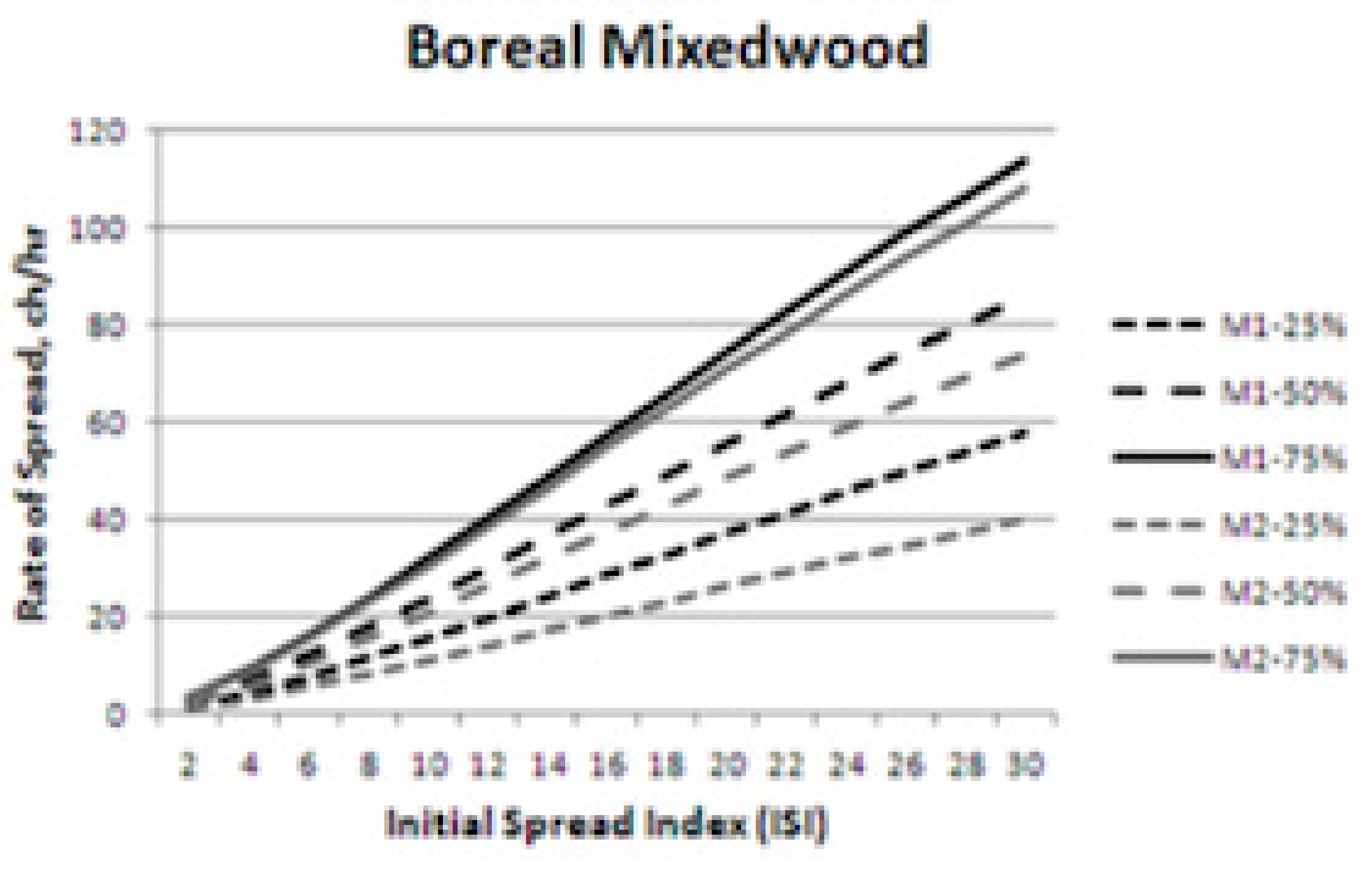
Fire 05 00016 i008
Figure A1. Conversion charts used to compare USA and Canada rate of spread (ROS) curves.
Fire 05 00016 g0a1

References

  1. Morris, G., III; Dennis, C. The 2020 Fire Siege; California Department of Forestry & Fire Protection: Sacramento, CA, USA, 2020. [Google Scholar]
  2. NIFC National Interagency Coordination Center. Wildland Fire Summary and Statistics Annual Report 2020. 2020. Available online: https://www.predictiveservices.nifc.gov/intelligence/2020_statssumm/annual_report_2020.pdf (accessed on 5 August 2021).
  3. California Departement of Water Resources (CA Dept. Water Resources). Water Year 2020 Summary Information. 2020; Volume 2020, pp. 1–4. Available online: https://water.ca.gov/-/media/DWR-Website/Web-Pages/What-We-Do/Drought-Mitigation/Files/Publications-And-Reports/Water-Year-2020-Handout_Final.pdf (accessed on 12 August 2021).
  4. Sommers, W.T.; Coloff, S.G.; Conard, S.G. Synthesis of Knowledge: Fire History and Climate Change; JFSP Synthesis Reports Paper 19; U.S. Joint Fire Science Program: Boise, ID, USA, 2011. Available online: https://www.firescience.gov/projects/09-2-01-11/project/09-2-01-11_pnw_gtr854.pdf (accessed on 5 January 2022).
  5. Perry, D.A.; Hessburg, P.F.; Skinner, C.N.; Spies, T.A.; Stephens, S.L.; Taylor, A.H.; Franklin, J.F.; McComb, B.; Riegel, G. The ecology of mixed severity fire regimes in Washington, Oregon, and Northern California. For. Ecol. Manag. 2011, 262, 703–717. [Google Scholar] [CrossRef]
  6. Parks, S.A.; Holsinger, L.M.; Panunto, M.H.; Jolly, W.M.; Dobrowski, S.Z.; Dillon, G.K. High-severity fire: Evaluating its key drivers and mapping its probability across western US forests. Environ. Res. Lett. 2018, 13, 44037. [Google Scholar] [CrossRef]
  7. Estes, B.L.; Knapp, E.E.; Skinner, C.N.; Miller, J.D.; Preisler, H.K. Factors influencing fire severity under moderate burning conditions in the Klamath Mountains, northern California, USA. Ecosphere 2017, 8, e01794. [Google Scholar] [CrossRef] [Green Version]
  8. Higuera, P.E.; Abatzoglou, J.T. Record-setting climate enabled the extraordinary 2020 fire season in the western United States. Glob. Change Biol. 2021, 27, 1–2. [Google Scholar] [CrossRef]
  9. Goss, M.; Swain, D.L.; Abatzoglou, J.T.; Sarhadi, A.; Kolden, C.A.; Williams, A.P.; Diffenbaugh, N.S. Climate change is increasing the likelihood of extreme autumn wildfire conditions across California. Environ. Res. Lett. 2020, 15, 94016. [Google Scholar] [CrossRef] [Green Version]
  10. Williams, A.P.; Abatzoglou, J.T.; Gershunov, A.; Guzman-Morales, J.; Bishop, D.A.; Balch, J.K.; Lettenmaier, D.P. Observed Impacts of Anthropogenic Climate Change on Wildfire in California. Earth’s Future 2019, 7, 892–910. [Google Scholar] [CrossRef] [Green Version]
  11. Ficklin, D.L.; Novick, K.A. Historic and projected changes in vapor pressure deficit suggest a continental-scale drying of the United States atmosphere. J. Geophys. Res. Atmos. 2017, 122, 2061–2079. [Google Scholar] [CrossRef]
  12. Abatzoglou, J.T.; Williams, A.P. Impact of anthropogenic climate change on wildfire across western US forests. Proc. Natl. Acad. Sci. USA 2016, 113, 11770–11775. [Google Scholar] [CrossRef] [Green Version]
  13. Westerling, A.L.; Bryant, B.P. Climate change and wildfire in California. Clim. Change 2007, 87, 231–249. [Google Scholar] [CrossRef]
  14. Keane, R.E. Fuel Moisture. Wildland Fuel Fundamentals and Application, 1st ed.; Springer: Cham, Switzerland, 2015; pp. 71–82. [Google Scholar] [CrossRef]
  15. Guirguis, K.; Gershunov, A.; Cayan, D.R.; Pierce, D.W. Heat wave probability in the changing climate of the Southwest US. Clim. Dyn. 2018, 50, 3853–3864. [Google Scholar] [CrossRef]
  16. Hulley, G.C.; Dousset, B.; Kahn, B.H. Rising Trends in Heatwave Metrics across Southern California. Earth’s Future 2020, 8, 1–21. [Google Scholar] [CrossRef]
  17. Pathak, T.B.; Maskey, M.L.; Dahlberg, J.A.; Kearns, F.; Bali, K.M.; Zaccaria, D. Climate change trends and impacts on California Agriculture: A detailed review. Agronomy 2018, 8, 25. [Google Scholar] [CrossRef] [Green Version]
  18. Gershunov, A.; Cayan, D.R.; Iacobellis, S.F. The great 2006 heat wave over California and Nevada: Signal of an increasing trend. J. Clim. 2009, 22, 6181–6203. [Google Scholar] [CrossRef] [Green Version]
  19. Diffenbaugh, N.S.; Swain, D.L.; Touma, D.; Lubchenco, J. Anthropogenic warming has increased drought risk in California. Proc. Natl. Acad. Sci. USA 2015, 112, 3931–3936. [Google Scholar] [CrossRef] [Green Version]
  20. Luković, J.; Chiang, J.C.H.; Blagojević, D.; Sekulić, A. A Later Onset of the Rainy Season in California. Geophys. Res. Lett. 2021, 48, 1–9. [Google Scholar] [CrossRef]
  21. Swain, D.L. A Shorter, Sharper Rainy Season Amplifies California Wildfire Risk. Geophys. Res. Lett. 2021, 48, e2021GL092843. [Google Scholar] [CrossRef]
  22. Tymstra, C. Development and Structure of Prometheus: The Canadian Wildland Fire Growth Simulation Model; NOR-X-417; Canadian Forest Service, Northern Forestry Centre: Ottawa, ON, Canada, 2010; Volume 417, ISBN 9781100146744. [Google Scholar]
  23. Opperman, T.; Gould, J.; Finney, M.; Tymstra, C. Applying Fire Spread Simulators in New Zealand and Australia: Results from an International Seminar; RMRS-P-41; US Department of Agriculture, Forest Service, Rocky Mountain Research Station: Fort Collins, CO, USA, 2006; Volume 41, pp. 201–212. Available online: http://www.fs.fed.us/rm/pubs/rmrs_p041/rmrs_p041_201_212.pdf (accessed on 20 August 2021).
  24. Forestry Canada Fire Danger Group. Development of the Canadian Forest Fire Behavior Prediction System; Information Report ST-X-3; Canadian Forest Service Publications: Sault Ste. Marie, ON, Canada, 1992; Volume 3, p. 66. Available online: https://cfs.nrcan.gc.ca/publications?id=10068%0Ahttps://www.frames.gov/documents/catalog/forestry_canada_fire_danger_group_1992.pdf (accessed on 12 January 2022).
  25. Wotton, B.M.; Alexander, M.E.; Taylor, S.W. Updates and Revisions to the 1992 Canadian Forest Fire Behavior Prediction System; Great Lakes Forestry Centre: Sault Ste. Marie, ON, Canada, 2009; ISBN 9781100114828. [Google Scholar]
  26. Incident Status Summary (ICS-209). National Wildfire Coordinating Group: Potomac, MD, USA, 2020. Available online: https://famit.nwcg.gov/applications/SIT209 (accessed on 12 January 2022).
  27. Hersbach, H.; Bell, B.; Berrisford, P.; Hirahara, S.; Horányi, A.; Muñoz-Sabater, J.; Nicolas, J.; Peubey, C.; Radu, R.; Schepers, D.; et al. The ERA5 global reanalysis. Q. J. R. Meteorol. Soc. 2020, 146, 1999–2049. [Google Scholar] [CrossRef]
  28. Picotte, J.J.; Long, J.; Peterson, B.; Nelson, K. LANDFIRE 2015 Remap—Utilization of Remotely Sensed Data to Classify Existing Vegetation Type and Structure to Support Strategic Planning and Tactical Response. Earthzine 2017, 2017, 1–6. [Google Scholar]
  29. Scott, J.H.; Burgan, R.E. Standard Fire Behavior Fuel Models: A Comprehensive Set for Use with Rothermel’s Surface Fire Spread Model; General Technical Report RMRS-GTR-153; United States Department of Agriculture Forest Service, Rocky Mountain Research Station: Fort Collins, CO, USA, 2005; pp. 1–76. [Google Scholar] [CrossRef]
  30. Fire Behavior Subcommittee. Fire Behavior Field Reference Guide, PMS 437. 2021. Available online: https://www.nwcg.gov/publications/437 (accessed on 5 December 2021).
  31. USFS. August Complex Briefing. 2020. Available online: https://inciweb.nwcg.gov/incident/article/6983/53484/ (accessed on 2 July 2021).
  32. Wilks, D.S. Statistical Methods in the Atmospheric Sciences, 3rd ed.; Elsevier Inc.: Oxford, UK, 2011; ISBN 978-0-12-385022-5. [Google Scholar]
  33. Rivera, J.D.D.; Davies, G.M.; Jahn, W. Flammability and the heat of combustion of natural fuels: A review. Combust. Sci. Technol. 2012, 184, 224–242. [Google Scholar] [CrossRef]
  34. Freeborn, P.H.; Jolly, W.M.; Cochrane, M.A.; Roberts, G. Large wildfire driven increases in nighttime fire activity observed across CONUS from 2003–2020. Remote Sens. Environ. 2022, 268, 112777. [Google Scholar] [CrossRef]
  35. Chiodi, A.M.; Potter, B.E.; Larkin, N.K. Multi-Decadal Change in Western US Nighttime Vapor Pressure Deficit. Geophys. Res. Lett. 2021, 48, e2021GL092830. [Google Scholar] [CrossRef]
  36. Davy, R.; Esau, I.; Chernokulsky, A.; Outten, S.; Zilitinkevich, S. Diurnal asymmetry to the observed global warming. Int. J. Climatol. 2017, 37, 79–93. [Google Scholar] [CrossRef] [Green Version]
  37. Keeley, J.E.; Syphard, A.D. Large California wildfires: 2020 fires in historical context. Fire Ecol. 2021, 17, 22. [Google Scholar] [CrossRef]
  38. Alexander, M.E.; Cruz, M.G. Assessing the effect of foliar moisture on the spread rate of crown fires. Int. J. Wildl. Fire 2013, 22, 415–427. [Google Scholar] [CrossRef]
  39. Byrne, M.P.; O’Gorman, P.A. Understanding Decreases in Land Relative Humidity with Global Warming: Conceptual Model and GCM Simulations. J. Clim. 2016, 29, 9045–9061. [Google Scholar] [CrossRef]
  40. Byrne, M.P.; O’Gorman, P.A. Trends in continental temperature and humidity directly linked to ocean warming. Proc. Natl. Acad. Sci. USA 2018, 115, 4863–4868. [Google Scholar] [CrossRef] [Green Version]
  41. Jain, P.; Castellanos-Acuna, D.; Coogan, S.C.P.; Abatzoglou, J.T.; Flannigan, M.D. Observed increases in extreme fire weather driven by atmospheric humidity and temperature. Nat. Clim. Change 2021, 12, 63–70. [Google Scholar] [CrossRef]
  42. Charney, J.J.; Potter, B.E. Convection and downbursts. Fire Manag. Today 2017, 75, 16–19. [Google Scholar]
  43. Steel, Z.L.; Safford, H.D.; Viers, J.H. The fire frequency-severity relationship and the legacy of fire suppression in California forests. Ecosphere 2015, 6, 1–23. [Google Scholar] [CrossRef]
  44. Srock, A.F.; Charney, J.J.; Potter, B.E.; Goodrick, S.L. The Hot-Dry-Windy Index: A new fireweather index. Atmosphere 2018, 9, 279. [Google Scholar] [CrossRef] [Green Version]
  45. Jolly, W.M.; Freeborn, P.H.; Page, W.G.; Butler, B.W. Severe fire danger index: A forecastable metric to inform firefighter and community wildfire risk management. Fire 2019, 2, 47. [Google Scholar] [CrossRef] [Green Version]
  46. Schlobohm, P.; Brain, J. Gaining an Understanding of the National Fire Danger Rating System; PMS 932; National Wildfire Coordinating Group: Potomac, MD, USA, 2002. Available online: https://www.nwcg.gov/sites/default/files/products/pms932.pdf (accessed on 15 November 2021).
  47. USDA Forest Service. The Rising Cost of Fire Operations: Effects on the Forest Service’s Non-Fire Work; USDA Forest Service: Washington, DC, USA, 2015; pp. 1–16. [Google Scholar]
  48. Ramírez, J.; Monedero, S.; Buckley, D. New approaches in fire simulations analysis with Wildfire Analyst. In Proceedings of the 7th international conference on forest fire research, Sun City, South Africa, 9–13 May 2011. [Google Scholar] [CrossRef]
  49. Cardil, A.; Monedero, S.; Ramírez, J.; Silva, C.A. Assessing and reinitializing wildland fire simulations through satellite active fire data. J. Environ. Manag. 2019, 231, 996–1003. [Google Scholar] [CrossRef] [PubMed]
Figure 1. The Doe Fire joined with several other smaller fires to form the August Complex, which burned 417,890 ha between 16 August and final containment on 15 November (mamsl = meters above mean sea level).
Fire 05 00016 g001
Figure 2. Observed (52,281 ha) and simulated (52,245 ha) Doe Fire perimeter on 22 August, after 96 h of explosive growth. ERA5 weather stream locations are marked with green locators.
Fire 05 00016 g002
Figure 3. (a) The four main fuels consumed during the DOE Fire simulation included very high load, dry climate shrub (SH7); very high load, dry climate timber-shrub (TU5); long-needle litter (TL8); and moderate load, dry climate shrub-grass (GS2). (b) Gridded rate of spread (ROS) output from the control with each day’s 1200 PDT perimeter.
Fire 05 00016 g003
Figure 4. (a) PC1 time series that highly correlates to (b) temperature, (c) ROS, (d) RH, and (e) meridional wind during the 96 h control run. PCA input variables are from the primary weather stream, the northwest location.
Fire 05 00016 g004
Figure 5. Observed (daily temporal resolution) and simulated (hourly resolution) Doe Fire growth compared to seven simulation experiments: (a) 41 years of climatologically averaged weather, (b) adding 0.8 °C to observed temperatures, (c) subtracting 0.8 °C, (d) adding 1.6 °C, (e) initializing fuel moisture content (FMC) with 41-year 90th percentile values of 17 August FMC, (f) changing ignition time to 08/05, pre-heatwave, and (g) changing ignition time to 09/06, hotter, drier heatwave.
Fire 05 00016 g005
Figure 6. Simulated heat release (HR) compared to seven simulation experiments: (a) 41 years of climatologically averaged weather, (b) adding 0.8 °C to observed temperatures, (c) subtracting 0.8 °C, (d) adding 1.6 °C, (e) initializing fuel moisture content (FMC) with 41-year 90th percentile values of 17 August FMC, (f) changing ignition time to 08/05, pre-heatwave, and (g) changing ignition time to 09/06, hotter, drier heatwave.
Fire 05 00016 g006
Figure 7. (a) Percent change in final fire area for each of the seven simulation experiments: 41 years of climatologically averaged weather, adding 0.8 °C to observed temperatures, subtracting 0.8 °C, adding 1.6 °C, initializing fuel moisture content (FMC) with 41-year 90th percentile values of 17 August FMC, changing ignition time to 08/05, pre-heatwave, and changing ignition time to 09/06, hotter, drier heatwave. (b) Percent change in total mean fire heat release (HR) for each experiment.
Fire 05 00016 g007
Figure 8. Depiction of how fire area changed with temperature variations (−0.8, 0.4, 0.8, 1.2, 1.6, 2.0, and 2.4 °C) compared to the control run. (a) The change in area with temperature adjustments and (b) that same area change against the mean vapor pressure deficit (VPD) for each scenario.
Fire 05 00016 g008
Table 1. Prometheus default values for required burning conditions and the values we used after calibration.
Required Burning ConditionsDefault ValueCalibrated Value
Initial Spread Index>6>6
Fire Weather Index>20>20
Wind Speed (km/h)>4>1.2
Relative Humidity (%)<25<40
Table 2. Results of the principal component analysis (PCA), showing the variance explained by each eigenvalue, as well as the correlations between each PC and temperature (T), relative humidity (RH), zonal winds (U), meridional winds (V), and rate of spread (ROS).
Variance ExplainedCorrelations
Eigenvalue% VarianceVariablesPC1PC2PC3PC4PC5
2.9458.77T0.920.04−0.210.20−0.25
1.0721.37RH−0.80−0.320.340.37−0.08
0.5410.88U−0.100.960.240.08−0.02
0.326.45V0.92−0.040.060.310.23
0.132.51ROS0.77−0.200.57−0.21−0.06
Table 3. Temperature (T), relative humidity (RH), vapor pressure deficit (VPD), wind speed (WS), fine fuel moisture code (FFMC), duff moisture code (DMC), drought code (DC), fire weather index (FWI), rate of spread (ROS), heat release (HR), and fire growth averaged over the main burning hours (1200–2200) for each day of the control run.
T
(°C)
RH
(%)
VPD (hPa)WS
(km/h)
FFMCDMCDCFWIROS
(m/min)
HR
(MW)
Growth (ha)
Day 132.917.142.26.192.645659036.34.5111181932
Day 229.512.937.09.094.246259846.06.63122211,172
Day 329.416.335.52.094.746760738.05.72124916,675
Day 429.330.129.53.394.247261538.04.6698912,917
Table 4. Mean temperature, relative humidity (RH), vapor pressure deficit (VPD), fine fuel moisture code (FFMC), duff moisture code (DMC), drought code (DC), and fire weather index (FWI) variables for each experimental simulation described in Figure 5, as well as the number of hours that each simulation actively spread.
ExperimentsT (°C)RH (%)VPDFFMCDMCDCFWI# Spreading Hours
Control25.328.525.790.146560329.348
Climatology23.234.520.489.540749226.743
Add 0.826.128.526.990.246760629.749
Add 1.626.928.528.290.447060930.150
Subtract 0.824.528.524.589.946260028.948
FMC 90th25.328.525.790.851450431.352
5-August24.737.721.488.339849025.036
6-September25.916.630.091.855775634.261
Publisher’s Note: MDPI stays neutral with regard to jurisdictional claims in published maps and institutional affiliations.

