
Detecting and Monitoring Early Post-Fire Sliding Phenomena Using UAV–SfM Photogrammetry and t-LiDAR-Derived Point Clouds

 ,
,  ,
, 
Abstract
:1. Introduction
1.1. Wildfires
1.2. Landslides
1.3. Early Landslide Phenomena and Detection Techniques—UAV Photogrammetry and t-Lidar
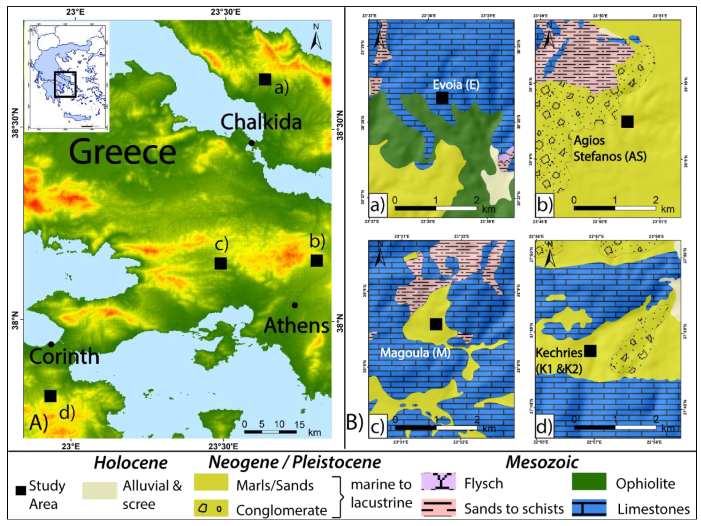
2. Study Areas
2.1. Evia
2.2. Agios Stefanos
2.3. Magoula
2.4. Kechries
3. Materials and Methods
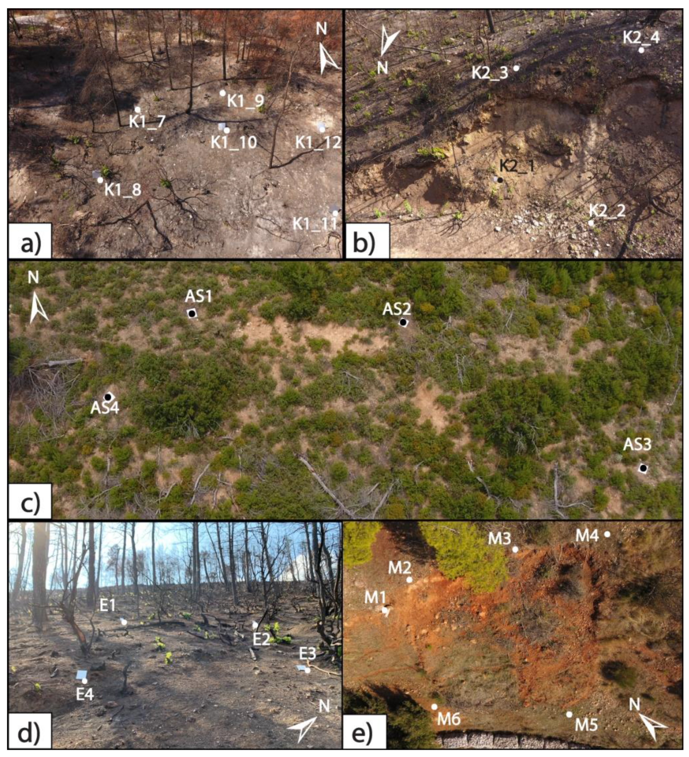
3.1. Selection and Characterisation of Landslide-Prone Areas
3.2. Data Acquisition
3.2.1. UAV Image Acquisition
3.2.2. t-LiDAR Scanning Characteristics
3.3. Data Processing
3.3.1. SfM Photogrammetry Processing
- Removal of photo metadata in order to remove the built-in GPS coordinates, as they were acquired in a different projection system than the RTK GNSS we used which might have caused decreased absolute accuracy of the model;
- Selection of all required photos in order to import them to the SfM software;
- Image alignment and development of Dense Point Cloud using high quality settings and mild filtering;
- Point classification and vegetation removal. The points corresponding to tree branches and trunks were classified as vegetation and removed from the point cloud;
- Development of mesh, texture and tiled models. The mesh was used for the creation of the DSM and the orthomosaic, while the texture and tiled models were used for the final check of our model and the easy distinction of the GCPs;
- Insertion of markers using the GCPs as a proxy. The markers were conventionally put in the lower right corner of each GCP, which were then surveyed accordingly;
- Markers error inspection using the software built-in routine and also by comparing known dimensions or absolute GCP locations (see also Section 3.4);
- Development of high-resolution DSM (Digital Surface Model) and orthomosaic of the whole scanned area. The maximum resolutions for the model, DSM and orthomosaic are displayed in Table 4;
- Extraction of Dense Point Cloud in order to use it in the CloudCompare software.
3.3.2. Point Cloud Processing
3.4. Error Estimation
4. Results
4.1. Evia
4.2. Kechries 1 & 2
4.3. Magoula
4.4. Ag. Stefanos
4.5. Summarised Results
4.6. Errors
5. Discussion
6. Conclusions
Author Contributions
Funding


Institutional Review Board Statement
Informed Consent Statement
Data Availability Statement
Conflicts of Interest
References
- Shakesby, R.; Doerr, S. Wildfire as a hydrological and geomorphological agent. Earth-Sci. Rev. 2006, 74, 269–307. [Google Scholar] [CrossRef]
- Shakesby, R. Post-wildfire soil erosion in the Mediterranean: Review and future research directions. Earth-Sci. Rev. 2011, 105, 71–100. [Google Scholar] [CrossRef]
- Cannon, S.H.; Kirkham, R.M.; Parise, M. Wildfire-related debris-flow initiation processes, Storm King Mountain, Colorado. Geomorphology 2001, 39, 171–188. [Google Scholar] [CrossRef]
- García-Ruiz, J.M.; Arnáez, J.; Gómez-Villar, A.; Ortigosa, L.; Lana-Renault, N. Fire-related debris flows in the Iberian Range, Spain. Geomorphology 2013, 196, 221–230. [Google Scholar] [CrossRef] [Green Version]
- Santi, P.; Cannon, S.; DeGraff, J. Wildfire and landscape change. In Geomorphology of Human Disturbances, Climate Change, and Natural Hazards; Shroder, J., James, L.A., Harden, C.P., Clague, J.J., Eds.; Treatise on Geomorphology; Academic Press: San Diego, CA, USA, 2013; Volume 13, pp. 262–287. [Google Scholar]
- Diakakis, M.; Nikolopoulos, E.I.; Mavroulis, S.; Vassilakis, E.; Korakaki, E. Observational evidence on the effects of mega-fires on the frequency of hydro-geomorphic hazards. The case of the Peloponnese fires of 2007 in Greece. Sci. Total Environ. 2017, 592, 262–276. [Google Scholar] [CrossRef] [PubMed]
- Santi, P.M.; Rengers, F.K. Wildfire and Landscape Change. In Reference Module in Earth Systems and Environmental Sciences; Elsevier BV: Amsterdam, The Netherlands, 2020. [Google Scholar] [CrossRef]
- Swanson, F.J. Fire and geomorphic processes. In Fire Regimes and Ecosystem Properties; Mooney, H.A., Bonnicksen, T.M., Christensen, N.L., Lotan, J.E., Reiners, W.A.Ž., Eds.; U.S. Department of Agriculture, Forest Service; Pacific Northwest Forest and Range Experiment Station: Corvallis, OR, USA, 1981; Volume 26, pp. 401–420. [Google Scholar]
- Cardinali, M.; Galli, M.; Guzzetti, F.; Ardizzone, F.; Reichenbach, P.; Bartoccini, P. Rainfall induced landslides in December 2004 in South-Western Umbria, Central Italy: Types, extent, damage and risk assessment. Nat. Hazards Earth Syst. Sci. 2006, 6, 237–260. [Google Scholar] [CrossRef]
- Chandler, J.; Brunsden, D. Steady-state behaviour of the Black Venmudslide: The application of archival analytical photogrammetry to studies of landform. Earth Surf. Process. Landf. 1995, 20, 255–275. [Google Scholar] [CrossRef]
- Gallousi, C.; Koukouvelas, I. Quantifying geomorphic evolution of earthquake-triggered landslides and their relation to active normal faults. An example from the Gulf of Corinth, Greece. Tectonophysics 2007, 440, 85–104. [Google Scholar] [CrossRef]
- Brardinoni, F.; Slaymaker, O.; Hassan, M.A. Landslide inventory in a rugged forested watershed: A comparison between air-photo and field survey data. Geomorphology 2003, 54, 179–196. [Google Scholar] [CrossRef]
- Mondini, A.C.; Guzzetti, F.; Chang, K.-T.; Monserrat, O.; Martha, T.R.; Manconi, A. Landslide failures detection and mapping using Synthetic Aperture Radar: Past, present and future. Earth-Sci. Rev. 2021, 216, 103574. [Google Scholar] [CrossRef]
- Sun, Q.; Hu, J.; Zhang, L.; Ding, X. Towards Slow-Moving Landslide Monitoring by Integrating Multi-Sensor InSAR Time Series Datasets: The Zhouqu Case Study, China. Remote Sens. 2016, 8, 908. [Google Scholar] [CrossRef] [Green Version]
- Qin, Y.; Hoppe, E.; Perissin, D. Slope Hazard Monitoring Using High-Resolution Satellite Remote Sensing: Lessons Learned from a Case Study. ISPRS Int. J. Geo-Inf. 2020, 9, 131. [Google Scholar] [CrossRef] [Green Version]
- Agüera-Vega, F.; Carvajal-Ramírez, F.; Martínez-Carricondo, P. Assessment of photogrammetric mapping accuracy based on variation ground control points number using unmanned aerial vehicle. Measurement 2017, 98, 221–227. [Google Scholar] [CrossRef]
- Agüera-Vega, F.; Carvajal-Ramírez, F.; Martínez-Carricondo, P.; Sánchez-Hermosilla López, J.; Mesas-Carrascosa, F.J.; García-Ferrer, A.; Pérez-Porras, F.J. Reconstruction of extreme topography from UAV structure from motion photogrammetry. Measurement 2018, 121, 127–138. [Google Scholar] [CrossRef]
- Valkaniotis, S.; Papathanassiou, G.; Ganas, A. Mapping an earthquake-induced landslide based on UAV imagery; case study of the 2015 Okeanos landslide, Lefkada, Greece. Eng. Geol. 2018, 245, 141–152. [Google Scholar] [CrossRef]
- Ardizzone, F.; Cardinali, M.; Galli, M.; Guzzetti, F.; Reichenbach, P. Identification and mapping of recent rainfall-induced landslides using elevation data collected by airborne Lidar. Nat. Hazards Earth Syst. Sci. 2007, 7, 637–650. [Google Scholar] [CrossRef] [Green Version]
- Niethammer, U.; Rothmund, S.; James, M.R.; Travelletti, J.; Joswig, M. UAV-based remote sensing of landslides. Int. Arch. Photogramm. Remote Sens. Spatial Inf. Sci. 2010, 38, 496–501. [Google Scholar]
- Niethammer, U.; James, M.R.; Rothmund, S. UAV-based remote sensing of the Super-Sauze landslide: Evaluation and results. Eng. Geol. 2012, 128, 2–11. [Google Scholar] [CrossRef]
- Colomina, I.; Molina, P. Unmanned aerial systems for photogrammetry and remote sensing: A review.ISPRS J. Photogramm. Remote Sens. 2014, 92, 79–97. [Google Scholar]
- Cheng, Z.; Gong, W.; Tang, H.; Juang, C.H.; Deng, Q.; Chen, J.; Ye, X. UAV photogrammetry-based remote sensing and preliminary assessment of the behavior of a landslide in Guizhou, China. Eng. Geol. 2021, 289, 106172. [Google Scholar] [CrossRef]
- Greif, V.; Vlcko, J. Monitoring of post-failure landslide deformation by the PS-InSAR technique at Lubietova in Central Slovakia. Environ. Earth Sci. 2011, 66, 1585–1595. [Google Scholar] [CrossRef]
- Strozzi, T.; Ambrosi, C.; Raetzo, H. Interpretation of Aerial Photographs and Satellite SAR Interferometry for the Inventory of Landslides. Remote Sens. 2013, 5, 2554–2570. [Google Scholar] [CrossRef] [Green Version]
- Li, X.; Cheng, X.; Chen, W.; Chen, G.; Liu, S. Identification of Forested Landslides Using LiDar Data, Object-based Image Analysis, and Machine Learning Algorithms. Remote Sens. 2015, 7, 9705–9726. [Google Scholar] [CrossRef] [Green Version]
- Morelli, S.; Pazzi, V.; Frodella, W.; Fanti, R. Kinematic Reconstruction of a Deep-Seated Gravitational Slope Deformation by Geomorphic Analyses. Geosci. 2018, 8, 26. [Google Scholar] [CrossRef] [Green Version]
- Eker, R.; Aydın, A. Long-term retrospective investigation of a large, deep-seated, and slow-moving landslide using InSAR time series, historical aerial photographs, and UAV data: The case of Devrek landslide (NW Turkey). Catena 2021, 196, 104895. [Google Scholar] [CrossRef]
- Delacourt, C.; Allemand, P.; Berthier, E.; Raucoules, D.; Casson, B.; Grandjean, P.; Pambrun, C.; Varel, E. Remote-sensing techniques for analysing landslide kinematics: A review. Bull. de La Société Géologique de Fr. 2007, 178, 89–100. [Google Scholar] [CrossRef]
- Casagli, N.; Frodella, W.; Morelli, S.; Tofani, V.; Ciampalini, A.; Intrieri, E.; Raspini, F.; Rossi, G.; Tanteri, L.; Lu, P. Spaceborne, UAV and ground-based remote sensing techniques for landslide mapping, monitoring and early warning. Geoenvironmental Disasters 2017, 4, 9. [Google Scholar] [CrossRef]
- Alexiou, S.; Deligiannakis, G.; Pallikarakis, A.; Papanikolaou, I.; Psomiadis, E.; Reicherter, K. Comparing High Accuracy t-LiDAR and UAV-SfM Derived Point Clouds for Geomorphological Change Detection. ISPRS Int. J. Geo-Inf. 2021, 10, 367. [Google Scholar] [CrossRef]
- Lucieer, A.; Turner, D.; King, D.H.; Robinson, S.A. Using an unmanned aerial vehicle (UAV) to capture micro-topography of antarctic moss beds. Int. J. Appl. Earth Obs. Geoinf. 2013, 27, 53–62. [Google Scholar] [CrossRef] [Green Version]
- Stumpf, A.; Malet, J.P.; Allemand, P. Ground-based multi-view photogrammetry for the monitoring of landslide deformation and erosion. Geomorphology 2015, 231, 130–145. [Google Scholar] [CrossRef]
- Al-Rawabdeh, A.; He, F.; Moussa, A.; El-Sheimy, N.; Habib, A. Using an Unmanned Aerial Vehicle-Based Digital Imaging System to Derive a 3D Point Cloud for Landslide Scarp Recognition. Remote Sens. 2016, 8, 95. [Google Scholar] [CrossRef] [Green Version]
- Clapuyt, F.; Vanacker, V.; Oost, K.V. Reproducibility of UAV-based earth topography reconstructions based on Structure-from-Motion algorithms. Geomorphology 2016, 260, 4–15. [Google Scholar] [CrossRef]
- Kucharczyk, M.; Hugenholtz, C.H. Remote sensing of natural hazard-related disasters with small drones: Global trends, biases, and research opportunities. Remote Sens. Environ. 2021, 264, 112577. [Google Scholar] [CrossRef]
- Antoine, R.; Lopez, T.; Tanguy, M.; Lissak, C.; Gailler, L.; Labazuy, P.; Fauchard, C. Geoscientists in the sky: Unmanned aerial vehicles responding to geohazards. Surv. Geophys. 2020, 41, 1285–1321. [Google Scholar] [CrossRef]
- Koukouvelas, I.Κ.; Nikolakopoulos, K.G.; Zygouri, V.; Kyriou, A. Post-seismic monitoring of cliff mass wasting using an unmanned aerial vehicle and field data at Egremni, Lefkada Island, Greece. Geomorphology 2020, 367, 107306. [Google Scholar] [CrossRef]
- Giordan, D.; Adams, M.S.; Aicardi, I.; Alicandro, M.; Allasia, P.; Baldo, M.; De Berardinis, P.; Dominici, D.; Godone, D.; Hobbs, P.; et al. The use of unmanned aerial vehicles (UAVs) for engineering geology applications. Bull. Eng. Geol. Environ. 2020, 79, 3437–3481. [Google Scholar] [CrossRef] [Green Version]
- Jaboyedoff, M.; Oppikofer, T.; Abell’an, A.; Derron, M.H.; Loye, A.; Metzger, R.; Pedrazzini, A. Use of LIDAR in landslide investigations: A review. Nat. Hazards 2012, 61, 5–28. [Google Scholar] [CrossRef] [Green Version]
- Lin, C.-W.; Tseng, C.-M.; Tseng, Y.-H.; Fei, L.-Y.; Hsieh, Y.-C.; Tarolli, P. Recognition of large scale deep-seated landslides in forest areas of Taiwan using high resolution topography. J. Asian Earth Sci. 2013, 62, 389–400. [Google Scholar] [CrossRef]
- Görüm, T. Landslide recognition and mapping in a mixed forest environment from airborne {LiDAR} data. Eng. Geol. 2019, 258, 105155. [Google Scholar] [CrossRef]
- Pánek, T.; Břežný, M.; Kapustová, V.; Lenart, J.; Chalupa, V. Large landslides and deep-seated gravitational slope deformations in the Czech Flysch Carpathians: New LiDAR-based inventory. Geomorphology 2019, 346, 106852. [Google Scholar] [CrossRef]
- Shi, W.; Deng, S.; Xu, W. Extraction of multi-scale landslide morphological features based on local Gi* using airborne LIDAR-derived DEM. Geomorphology 2018, 303, 229–242. [Google Scholar] [CrossRef]
- Syzdykbayev, M.; Karimi, B.; Karimi, H.A. Persistent homology on LiDAR data to detect landslides. Remote Sens. Environ. 2020, 246, 111816. [Google Scholar] [CrossRef]
- Eltner, A.; Baumgart, P.; Maas, H.G.; Faust, D. Multi-temporal UAV data for automatic measurement of rill and interrill erosion on loess soil. Earth Surf. Process. Landf. 2015, 40, 741–755. [Google Scholar] [CrossRef]
- Peppa, M.; Mills, J.P.; Moore, P.; Miller, P.E.; Chambers, J.C. Accuracy assessment of a UAV-based landslide monitoring system. Int. Arch. Photogramm. Remote Sens. Spat. Inf. Sci. 2016, 41, 895–902. [Google Scholar]
- Yang, D.; Qiu, H.; Hu, S.; Pei, Y.; Wang, X.; Du, C.; Long, Y.; Cao, M. Influence of successive landslides on topographic changes revealed by multitemporal high-resolution UAS-based DEM. Catena 2021, 202, 105229. [Google Scholar] [CrossRef]
- Rothmund, S.; Vouillamoz, N.; Joswig, M. Mapping slow-moving alpine landslides by UAV-Opportunities and limitations. Lead. Edge 2017, 36, 571–579. [Google Scholar] [CrossRef]
- Wang, H.; Nie, D.; Tuo, X.; Zhong, Y. Research on crack monitoring at the trailing edge of landslides based on image processing. Landslides 2020, 17, 985–1007. [Google Scholar] [CrossRef]
- Chae, B.-G.; Park, H.-J.; Catani, F.; Simoni, A.; Berti, M. Landslide prediction, monitoring and early warning: A concise review of state-of-the-art. Geosci. J. 2017, 21, 1033–1070. [Google Scholar] [CrossRef]
- Cignetti, M.; Godone, D.; Wrzesniak, A.; Giordan, D. Structure from motion multisource application for landslide characterisation and monitoring: The champlas du col case study, sestriere, North-Western Italy. Sensors 2019, 19, 2364. [Google Scholar] [CrossRef] [PubMed] [Green Version]
- Nappo, N.; Mavrouli, O.; Nex, F.; van Westen, C.; Gambillara, R.; Michetti, A.M. Use of UAV-based photogrammetry products for semi-automatic detection and classification of asphalt road damage in landslide-affected areas. Eng. Geol. 2021, 294, 106363. [Google Scholar] [CrossRef]
- Mateos, R.M.; López-Vinielles, J.; Bru, G.; Sarro, R.; Béjar-Pizarro, M.; Herrera, G. Landslides in Urban Environments. Ref. Modul. Earth Syst. Environ. Sci. 2021. [Google Scholar] [CrossRef]
- Carabella, C.; Miccadei, E.; Paglia, G.; Sciarra, N. Post-Wildfire Landslide Hazard Assessment: The Case of The 2017 Montagna Del Morrone Fire (Central Apennines, Italy). Geosciences 2019, 9, 175. [Google Scholar] [CrossRef] [Green Version]
- Rengers, F.K.; McGuire, L.A.; Oakley, N.S.; Kean, J.W.; Staley, D.M.; Tang, H. Landslides after wildfire: Initiation, magnitude, and mobility. Landslides 2020, 17, 2631–2641. [Google Scholar] [CrossRef]
- Bornovas, J.; Lalechos, N.; Filipakis, N. Geological Map of Greece, Korinthos Sheet 1.50.000, I.G.M.E., Athens. 1972.
- Katsikatsos, G.; Koukis, G.; Fytikas, M. Geological Map of Greece, Psachna-Pilion Sheet 1.50.000, I.G.M.E., Athens. 1981.
- Katsikatsos, G.; Dounas, A.; Gaitanakis, P. Geological Map of Greece, Athinai–Elefsis Sheet 1.50.000, I.G.M.E., Athens. 1986.
- Katsikatsos, G. Geological Map of Greece. Kifisia Sheet 1.50.000, I.G.M.E., Athens. 2002.
- Bolle, H.-J. (Ed.) Mediterranean Climate: Variability and Trends; Springer: Heidelberg, Geramny, 2003. [Google Scholar]
- Giannakopoulos, C.; Kostopoulou, E.; Varotsos, K.V.; Tziotziou, K.; Plitharas, A. An integrated assessment of climate change impacts for Greece in the near future. Reg. Environ. Chang. 2011, 11, 829–843. [Google Scholar] [CrossRef] [Green Version]
- Koutsoyiannis, D.; Baloutsos, G. Analysis of a long record ofannual maximum rainfall in Athens, Greece, and design rainfallinferences. Nat. Hazards 2000, 29, 29–48. [Google Scholar] [CrossRef]
- National Observatory of Athens (NOA). Available online: https://www.meteo.gr/ (accessed on 30 October 2021).
- Markonis, Y.; Batelis, S.C.; Dimakos, Y.; Moschou, E.C.; Koutsoyiannis, D. Temporal and spatial variability of rainfall over Greece. Theor. Appl. Climatol. 2016, 130, 2016–2232. [Google Scholar] [CrossRef]
- European Forest Fire Information System (EFFIS). Available online: http://effis.jrc.ec.europa.eu/applications/data-request-form/ (accessed on 28 September 2020).
- CLMS. Copernicus land monitoring service datasets. 2016. Available online: http://land.copernicus.eu/pan-european/corine-land-cover (accessed on 28 September 2020).
- Marinos, P.; Boukovalas, G.; Tsiambaos, G.; Protonotarios, G.; Sabatakakis, N. Preliminary Geological—Geotechnical Study of the Disaster Area (of Athens Earthquake of 7 September 1999) in NW Athens Basin (in Greek) E.P.P.O., Athens, (13 pp.). 1999.
- Keeley, J.E. Fire intensity, fire severity and burn severity: A brief review and suggested usage. Int. J. Wildland Fire 2009, 18, 116–126. [Google Scholar] [CrossRef]
- Rusnák, M.; Sládek, J.; Kidová, A.; Lehotský, M. Template for high-resolution river landscape mapping using UAV technology—Institute of Geography. Slovak Acad. Sci. Štefániková 2017, 49, 814. [Google Scholar]
- James, M.R.; Robson, S.; Smith, M.W. 3-D uncertainty-based topographic change detection with structure-from-motion photogrammetry: Precision maps for ground controland directly georeferenced surveys. Earth Surf. Process. Landf. 2017, 42, 1769–1788. [Google Scholar] [CrossRef]
- James, M.; Robson, S.; D’Oleire-Oltmanns, S.; Niethammer, U. Optimising UAV topographic surveys processed with structure-from-motion: Ground control quality, quantity and bundle adjustment. Geomorphology 2017, 280, 51–66. [Google Scholar] [CrossRef] [Green Version]
- Miřijovský, J.; Langhammer, J. Multitemporal Monitoring of the Morphodynamics of a Mid-Mountain Stream Using UAS Photogrammetry. Remote Sens. 2015, 7, 8586–8609. [Google Scholar] [CrossRef] [Green Version]
- Tamminga, A.D.; Eaton, B.C.; Hugenholtz, C.H. UAS-based remote sensing of fluvial change following an extreme flood event. Earth Surf. Process. Landf. 2015, 40, 1464–1476. [Google Scholar] [CrossRef]
- Andreadakis, E.; Diakakis, M.; Vassilakis, E.; Deligiannakis, G.; Antoniadis, A.; Andriopoulos, P.; Spyrou, N.; Nikolopoulos, E. Unmanned Aerial Systems-Aided Post-Flood Peak Discharge Estimation in Ephemeral Streams. Remote Sens. 2020, 12, 4183. [Google Scholar] [CrossRef]
- Marteau, B.; Vericat, D.; Gibbins, C.; Batalla, R.J.; Green, D.R. Application of Structure-from-Motion photogrammetry to river restoration. Earth Surf. Process. Landf. 2017, 42, 503–515. [Google Scholar] [CrossRef] [Green Version]
- Ferrer-González, E.; Agüera-Vega, F.; Carvajal-Ramírez, F.; Martínez-Carricondo, P. UAV Photogrammetry Accuracy Assessment for Corridor Mapping Based on the Number and Distribution of Ground Control Points. Remote Sens. 2020, 12, 2447. [Google Scholar] [CrossRef]
- Martínez-Carricondo, P.; Agüera-Vega, F.; Carvajal-Ramírez, F.; Mesas-Carrascosa, F.J.; García-Ferrer, A.; Pérez-Porras, F.-J. Assessment of UAV-photogrammetric mapping accuracy based on variation of ground control points. Int. J. Appl. Earth Obs. Geoinf. 2018, 72, 1–10. [Google Scholar] [CrossRef]
- Zhang, W.; Qi, J.; Wan, P.; Wang, H.; Xie, D.; Wang, X.; Yan, G. An Easy-to-Use Airborne LiDAR Data Filtering Method Based on Cloth Simulation. Remote Sens. 2016, 8, 501. [Google Scholar] [CrossRef]
- Lague, D.; Brodu, N.; Leroux, J. Accurate 3D comparison of complex topographywith terrestrial laser scanner: Application to the Rangitikei canyon (N-Z). ISPRSJ. Photogramm. Remote Sens. 2013, 82, 10–26. [Google Scholar]
- D’Oleire-Oltmanns, S.; Marzolff, I.; Peter, K.D.; Ries, J.B. Unmanned aerial vehicle (UAV) for monitoring soil erosion in Morocco. Remote Sens. 2012, 4, 3390–3416. [Google Scholar] [CrossRef] [Green Version]
- Zhu, X.; Xu, Q.; Qi, X.; Liu, H. A self-adaptive data acquisition technique and its application in landslide monitoring. In Advancing Culture of Living with Landslides; Springer: Cham, Switzerland, 2017; pp. 71–78. [Google Scholar]
- Lainas, S.; Sabatakakis, N.; Koukis, G. Rainfall thresholds for possible landslide initiation in wildfire-affected areas of western Greece. Bull. Int. Assoc. Eng. Geol. 2016, 75, 883–896. [Google Scholar] [CrossRef]
- Guzzetti, F.; Peruccacci, S.; Rossi, M.; Stark, C.P. Rainfall thresholds for the initiation of landslides in central and southern Europe. Meteorol. Atmos. Phys. 2007, 98, 239–267. [Google Scholar] [CrossRef]
- Nastos, P.T.; Moustris, K.P.; Larissi, I.K.; Paliatsos, A.G. Rain intensity forecast usingArtificial Neural Networks in Athens, Greece. Atmos. Res. 2013, 119, 153–160. [Google Scholar] [CrossRef]
- Tournadre, V.; Pierrot-Deseilligny, M.; Faure, P.H. UAV Photogrammetry to Monitor Dykes–Calibration and Comparison to Terrestrial LiDAR. EuroCOW 2014, the European Calibration and Orientation Workshop; ISPRS (International Archives of the Photogrammetry, Remote Sensing and Spatial Information Sciences): Castelldefels, Spain, 2014; pp. 143–148. [Google Scholar]
- Brede, B.; Lau, A.; Bartholomeus, H.M.; Kooistra, L. Comparing RIEGL RiCOPTER UAV LiDAR Derived Canopy Height and DBH with Terrestrial LiDAR. Sensors 2017, 17, 2371. [Google Scholar] [CrossRef] [PubMed]
- Vilbig, J.M.; Sagan, V.; Bodine, C. Archaeological surveying with airborne LiDAR and UAV photogrammetry: A comparative analysis at Cahokia Mounds. J. Archaeol. Sci. Rep. 2020, 33, 102509. [Google Scholar] [CrossRef]
- Fernández, C.; Vega, J.A. Efficacy of bark strands and straw mulching after wildfire in NW Spain: Effects on erosion control and vegetation recovery. Ecol. Eng. 2014, 63, 50–57. [Google Scholar] [CrossRef]
- Fernández, C.; Vega, J.A.; Fontúrbel, T. Does helimulching after severe wildfire affect vegetation recovery in a coastal area of Northwest Spain? Landsc. Ecol. Eng. 2019, 15, 337–345. [Google Scholar] [CrossRef]


| Location | Jan | Feb | Mar | Apr | May | Jun | Jul | Aug | Sep | Oct | Nov | Dec | Total |
|---|---|---|---|---|---|---|---|---|---|---|---|---|---|
| Evia | |||||||||||||
| 2019 | 121.8 | 123.2 | 7 | 0 | 0 | 0 | 0.2 | 0 | 0 | 0 | 0.2 | 213.4 | 465.8 |
| 2020 | 86.4 | 92.4 | 46.2 | 122.4 | 15.6 | 15.4 | 0 | 226 | 15.2 | 31 | 47.4 | 118 | 818 |
| 2021 | 53.8 | 78.2 | 26 | 25.8 | 1.2 | 19.4 | 0 | 5.2 | 29 | 59.6 | - | - | 298.2 |
| Ag. Stefanos | |||||||||||||
| 2019 | 183.2 | 140.6 | 36.2 | 114 | 2.2 | 0 | 43 | 0 | 4.2 | 34 | 194.8 | 243.8 | 996 |
| 2020 | 112.3 | 77 | 106.2 | 68.6 | 71.4 | 44.2 | 0 | 15.2 | 39.4 | 50.8 | 29.8 | 238.8 | 853.7 |
| 2021 | 88.8 | 38.8 | 29.8 | 27.8 | 0.4 | 15.2 | 1.2 | 9.2 | 5.6 | 158.8 | - | - | 375.6 |
| Magoula | |||||||||||||
| 2019 | 89.6 | 46.2 | 16.6 | 71.2 | 1.4 | 8 | 3.4 | 0 | 4.2 | 20 | 108 | 123.8 | 492.4 |
| 2020 | 45.8 | 22.6 | 41.8 | 33.6 | 37.4 | 16.2 | 0.4 | 27.4 | 5 | 31.6 | 7 | 156 | 424.6 |
| 2021 | 82 | 23 | 7.6 | 19.8 | 0 | 18.6 | 0 | 0 | 1.4 | 125 | - | - | 277.4 |
| Kechries | |||||||||||||
| 2019 | 159.4 | 82.6 | 49.4 | 50.8 | 1 | 14.4 | 76.2 | 0 | 4 | 42.4 | 178 | 42.4 | 700.6 |
| 2020 | 12.2 | 5.6 | 76.6 | 76 | 25.6 | 6 | 0 | 10.6 | 26.2 | 14.2 | 15.8 | 73.4 | 342.2 |
| 2021 | 47.6 | 21 | 6.4 | 11.6 | 2.2 | 36.2 | 0 | 0 | 0.4 | 53.6 | - | - | 179 |
| Site Name | Date | Number of Photos | Mean Flight Altitude (AGL) | Mean Slope |
|---|---|---|---|---|
| Evia | 19/10/2019 | 298 | 5–15 m | 30° |
| Evia | 23/2/2020 | 217 | 5–15 m | 30° |
| Ag. Stefanos | 9/10/2019 | 142 | 20–35 m | 38° |
| Ag. Stefanos | 13/6/2020 | 242 | 20–35 m | 38° |
| Magoula | 9/11/2019 | 351 | 5–10 m | 25° |
| Magoula | 13/6/2020 | 401 | 5–10 m | 25° |
| Kechries (K1) | 29/8/2020 | 411/- | 3–15 m | 27° |
| Kechries (K1/K2) | 8/10/2020 | 432/93 | 3–15 m | 27°/29° |
| Kechries (K1/K2) | 24/3/2021 | 395/134 | 5–15 m | 27°/29° |
| Site Name | Date | Mean Distance (m) | Beam Width (mm) | Pulse Mode | Spacing (mm) |
|---|---|---|---|---|---|
| Evia | 19/10/2019 | 8.22 | 14 | last | 7.1 |
| Evia | 23/2/2020 | 10 | 14 | last | 7.1 |
| Ag. Stefanos | 13/06/2020 | 127 | 14 | last | 28 |
| Magoula | 13/06/2020 | 39.5 | 14 | last | 12 |
| Kechries | 29/08/2020 | 27 | 14 | last | 11 |
| Kechries | 08/10/2020 | 25 | 14 | last | 10 |
| Kechries | 14/03/2021 | 25 | 14 | last | 10 |
| Maximum Resolution mm/pix | |||
|---|---|---|---|
| Tiled Model | DEM | Orthomosaic | |
| Ag. Stefanos | 7.7 | 15.4 | 7.7 |
| Magoula | |||
| 9/11/2019 | 3.2 | 6.4 | 3.2 |
| 20/6/2020 | 4.1 | 8.4 | 4.2 |
| C. Evia | |||
| 19/10/2019 | 3.7 | 7.3 | 3.6 |
| 23/02/2020 | 2.3 | 4.7 | 2.3 |
| Kechries (K1/K2) | |||
| 29/8/2020 | 6.1/- | 12.3/ - | 6.13/ - |
| 8/10/2020 | 6.8/ 3.5 | 13.5/7.0 | 6.7/ 3.5 |
| 14/3/2021 | 3.6/3 | 7.2/5.8 | 3.5/3 |
| Site Name | Qualitative | Quantitative |
|---|---|---|
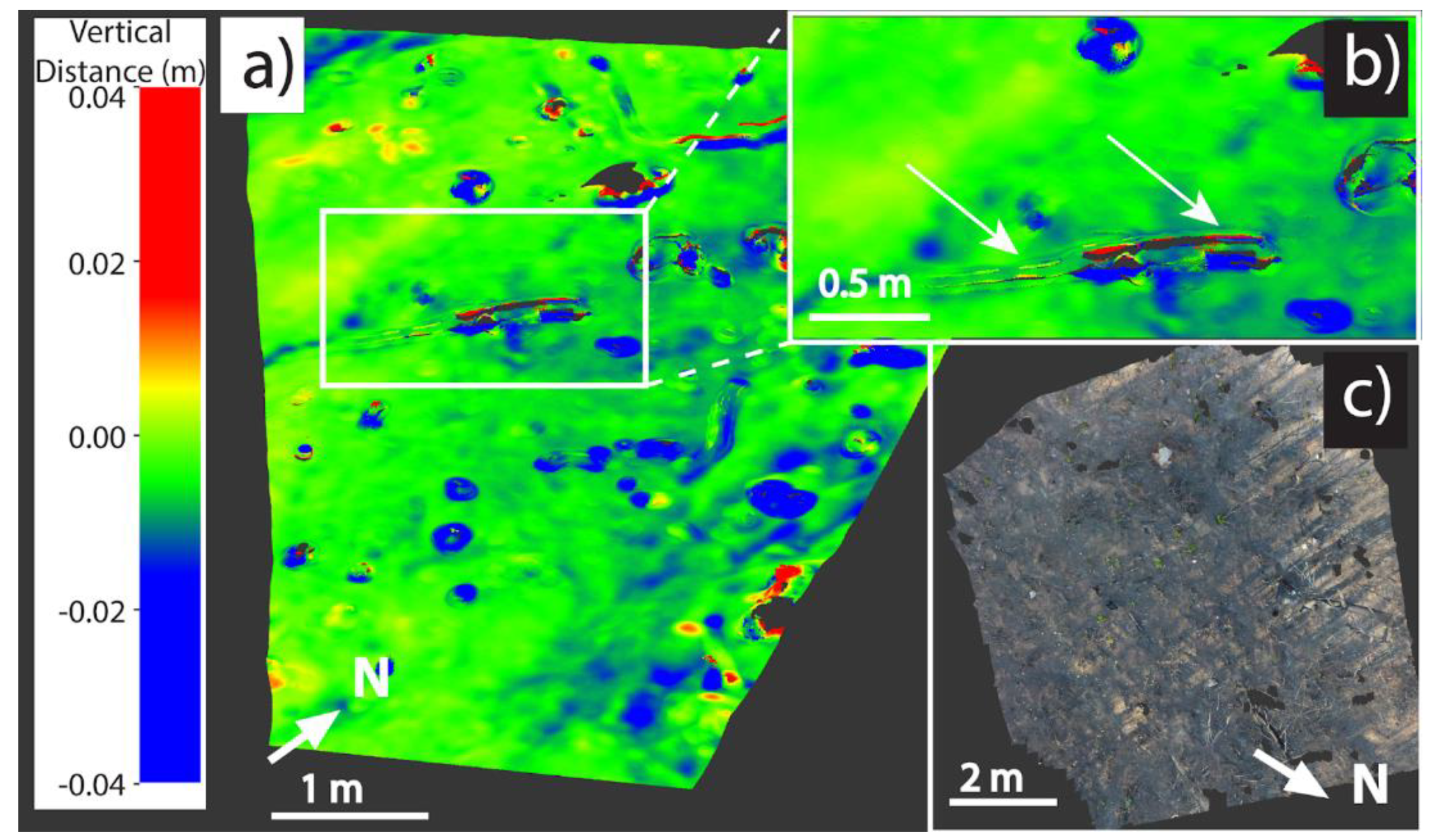
| Evia | New crack | ~ 4–5 ± 3 cm high and 1.5 m long |
| Ag. Stefanos | Description of pre-existing landslide | No measured displacement |
| Magoula | Expansion of pre-existing landslide | ~8 % expansion of the landslide |
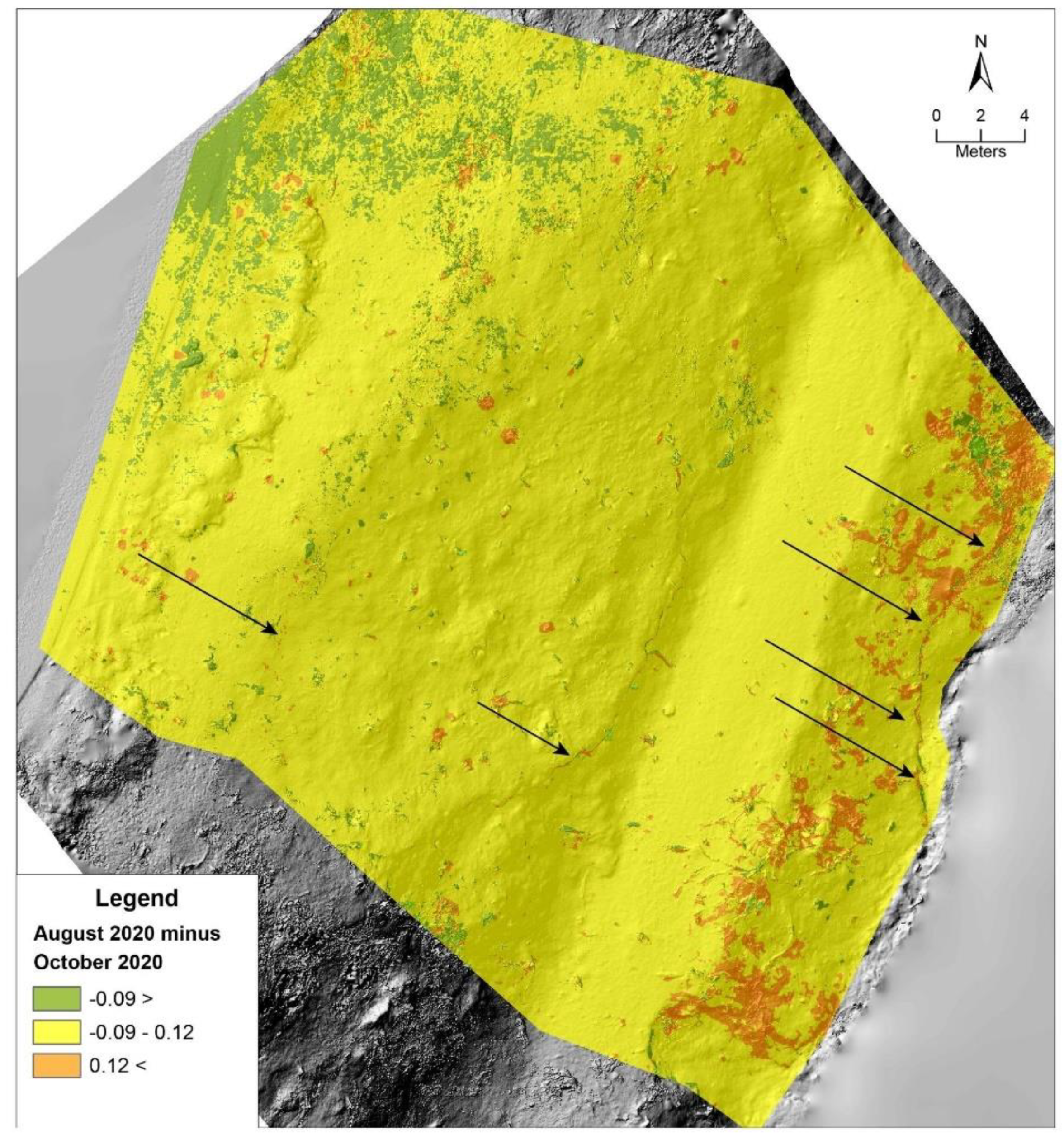
| Kechries one | Expansion of pre-existing crack & New cracks | From ~10 ± 4 cm (smaller cracks) to ~19 ± 4 cm (major crack) with lateral expansion up to ~ 27.5 m |
| Kechries two | Expansion of preexisting scarp | ~10–15 ± 4 cm high |
| Site Name | Date | DSM Mean Error (m) | GNSS—XYZ Error (m) | GCP Registration Error (m) | Feature Alignment Error (m) |
|---|---|---|---|---|---|
| Evia (TLS) | 19/10/2019 | - | 0.02 (based on SP60 measurements) | 0.03 | 0.01 |
| Evia (UAV-SfM) | 19/10/2019 | 0.041 | 0.02 (based on SP60 measurements) | 0.02 | 0.01 |
| Evoia (TLS) | 23/02/2020 | - | 0.02 (based on SP60 measurements) | 0.03 | 0.01 |
| Evia (UAV-SfM) | 23/02/2020 | 0.045 | 0.02 (based on SP60 measurements) | 0.02 | 0.01 |
| Magoula (TLS) | 13/06/2020 | - | 0.018 (based on SP60 measurements) | 0.07 | - |
| Magoula (UAV-SfM) | 13/06/2020 | 0.052 | 0.018 (based on SP60 measurements) | 0.03 | - |
| Ag. Stefanos (TLS) | 13/06/2021 | - | 0.018 (based on SP60 measurements) | 0.10 | - |
| Ag. Stefanos (UAV -SfM) | 13/06/2021 | 0.058 | 0.018 (based on SP60 measurements) | 0.02 | - |
| Kechries one (UAV-SfM) | 29/08/2020 | 0.039 | 0.04 | 0.03 | 0.02 |
| Kechries one (TLS) | 29/08/2020 | - | 0.04 | 0.05 | 0.02 |
| Kechries one (TLS) | 08/10/2020 | - | 0.03 | 0.05 | 0.02 |
| Kechries one (UAV-SfM) | 08/10/2020 | 0.038 | 0.04 | 0.04 | 0.02 |
| Kechries two (UAV-SfM) | 08/10/2020 | 0.043 | 0.003 (based on target measurements) | 0.01 | - |
| Kechries one (UAV-SfM) | 14/03/2021 | 0.049 | 0.015 | 0.01 | 0.02 |
| Kechries one (TLS) | 14/03/2021 | 0.047 | 0.02 | 0.05 | 0.02 |
| Kechries two (UAV-SfM) | 14/03/2021 | 0.043 | 0.003 (based on target measurements) | 0.01 | - |
Publisher’s Note: MDPI stays neutral with regard to jurisdictional claims in published maps and institutional affiliations. |
© 2021 by the authors. Licensee MDPI, Basel, Switzerland. This article is an open access article distributed under the terms and conditions of the Creative Commons Attribution (CC BY) license (https://creativecommons.org/licenses/by/4.0/).
Share and Cite
Deligiannakis, G.; Pallikarakis, A.; Papanikolaou, I.; Alexiou, S.; Reicherter, K. Detecting and Monitoring Early Post-Fire Sliding Phenomena Using UAV–SfM Photogrammetry and t-LiDAR-Derived Point Clouds. Fire 2021, 4, 87. https://doi.org/10.3390/fire4040087
Deligiannakis G, Pallikarakis A, Papanikolaou I, Alexiou S, Reicherter K. Detecting and Monitoring Early Post-Fire Sliding Phenomena Using UAV–SfM Photogrammetry and t-LiDAR-Derived Point Clouds. Fire. 2021; 4(4):87. https://doi.org/10.3390/fire4040087
Chicago/Turabian StyleDeligiannakis, Georgios, Aggelos Pallikarakis, Ioannis Papanikolaou, Simoni Alexiou, and Klaus Reicherter. 2021. "Detecting and Monitoring Early Post-Fire Sliding Phenomena Using UAV–SfM Photogrammetry and t-LiDAR-Derived Point Clouds" Fire 4, no. 4: 87. https://doi.org/10.3390/fire4040087
APA StyleDeligiannakis, G., Pallikarakis, A., Papanikolaou, I., Alexiou, S., & Reicherter, K. (2021). Detecting and Monitoring Early Post-Fire Sliding Phenomena Using UAV–SfM Photogrammetry and t-LiDAR-Derived Point Clouds. Fire, 4(4), 87. https://doi.org/10.3390/fire4040087