Abstract
Burning firebrands generated by wildland or prescribed fires may lead to the initiation of spot fires and fire escapes. At the present time, there are no methods that provide information on the thermal characteristics and number of such firebrands with high spatial and temporal resolution. A number of algorithms have been developed to detect and track firebrands in field conditions in our previous study; however, each holds particular disadvantages. This work is devoted to the development of new algorithms and their testing and, as such, several laboratory experiments were conducted. Wood pellets, bark, and twigs of pine were used to generate firebrands. An infrared camera (JADE J530SB) was used to obtain the necessary thermal video files. The thermograms were then processed to create an annotated IR video database that was used to test both the detector and the tracker. Following these studies, the analysis showed that the Difference of Gaussians detection algorithm and the Hungarian tracking algorithm upheld the highest level of accuracy and were the easiest to implement. The study also indicated that further development of detection and tracking algorithms using the current approach will not significantly improve their accuracy. As such, convolutional neural networks hold high potential to be used as an alternative approach.
1. Introduction
Prescribed fire is a tool that is widely used by fire managers in order to reduce fuel build-up and decrease the likelihood of high-intensity fires around communities [1,2,3,4,5]. On some occasions, prescribed fires escape and can cause significant impact on communities and biodiversity [6]. Spotting is often the known cause of escapes and, as a result, frequently overwhelms fire suppression efforts, in turn breaching large barriers and firebreaks [7]. Burning firebrands that are produced in the fire front and further transported by wind can also ignite structures in wildland-urban interface (WUI) areas [8,9,10,11,12,13]. Prescribed fire escapes and WUI fires are expected to pose serious future threats due to climate change [14] and individual preferences to live close to forested areas [15].
At present, there is a prominent need to determine a quantitative understanding of the short distance spotting dynamics, namely the firebrand distribution within a distance from the fire front and the way(s) in which fires coalesce. The absence of such data proves to be an obstacle to the development of fire hazard forecasting methods, as well as to the improvement of measures and recommendations for more efficient and effective work to prevent, control, and extinguish prescribed and surface fires, as well as to minimize the risk of ignition of residential buildings.
Recently, several studies have been conducted in an attempt to solve this problem [16,17,18,19,20,21,22,23]. In order to conduct this research, a series of prescribed fire experiments within pine forests were performed to study the generation of firebrands and their properties as a function of fire behavior [16,17,18]. Hedayati et al. [20] conducted experiments that were designed to generate firebrands from building materials in a wind tunnel and, upon doing so, proposed a probabilistic model for the estimation of firebrand mass/projected area/flying distance. The formation of firebrands from thermally degraded vegetative elements was also investigated in the study [19]. [23] used 3D Particle Tracking Velocimetry and 3D Particle Shape Reconstruction to reconstruct 3D models of individual particles and their trajectories. Additionally, particle tracking velocimetry and flame front detection techniques were also tested to explore [21] commercial aircraft debris striking. One study [22] presented a methodology that combined color-ratio pyrometry and particle streak-tracking velocimetry, together with digital image processing, in order to obtain non-intrusive measurements of the temperature, velocity, and size of multiple sparks in a spray. Despite the existing studies, a reliable method for obtaining the thermal and physical characteristics of firebrands in both laboratory and field conditions has not yet been developed.
In order to address this, an initial version of custom software was developed with the aim of detecting the location and number of flying firebrands in a thermal image, and further determining the temperature and sizes of each firebrand [24]. The software consists of two modules: the detector and the tracker. The detector determines the location of firebrands in the frame, and the tracker compares a firebrand in different frames and determines the identification number of each firebrand. However, used algorithms had certain disadvantages, namely that the detector and tracker were both developed and calibrated for a low frame rate (frames per second or FPS) and a low number of particles.
In this regard, this work is devoted to the development of new algorithms and their testing process by utilizing laboratory experimental data.
2. Materials and Methods
2.1. Development of GUI
A graphical user interface (GUI) was developed to work alongside software for detecting, tracking, and determining the characteristics of burning firebrands. To develop the GUI, available libraries of graphic elements that support the used software language of Python3 were considered and compared [25]. In particular, the libraries Tkinter, pyGTK/PyGObject, wxPython, and pyQt5 were highlighted. The subsequent choice was made in favor of the PyQt5 library, largely due to its ability to work with the Qt cross-platform framework, which allows applications to be run under various operating systems (Windows, MacOS X, Linux). To render the video frames, a free graphic component library Qwt, which works in conjunction with a library Qt, was used. This library provides both animation and the scaling of data, and the graphical interface is used to open and visualize videos in the ASCII frame format.
2.2. Testing Algorithms
Detector testing. To detect burning firebrands in the frame, various Gaussian convolution algorithms were tested, namely the Laplacian of Gaussian (LoG) and the Difference of Gaussian (DoG). These algorithms were aimed towards the identification of projected areas.
The LoG algorithm is based on the convolution (filtering) of an image using the Laplace operator:
here is the Gaussian kernel, is the Gaussian parameter, are spatial coordinates.
The LoG can be given by the formula
where is the LoG filter.
The DoG algorithm is based on two convolutions of the Gaussian image with the different parameter of σ.
where and are the Gaussian kernels.
The second step of the algorithm is the pixel-by-pixel subtraction of the Gaussian images from each other.
where is the DoG filter.
To evaluate the accuracy of the detectors, the F1 score was used [26]:
where TP is the number of true positives, FP is the number of false positives, and FN is the number of false negatives.
This metric takes into account two types of false positives: (i) when a background element is falsely detected (false operation); (ii) when a visible particle is not detected.
Tracker Testing. After detecting all particles in the frame, it is necessary to then determine whether it is a new particle or if it is in the previous frame, and then assign the particle a unique identification number. For this purpose, special particle trackers were developed.
In the previous version of the software [24], the tracker was based upon the nearest neighbor search method (NSS) [27]. Each detection in the current frame, according to the selected metric, was compared to the detection in the next frame, whilst all other detections were ignored. The advantages of this tracker include simple implementation, high operation speed, and low memory consumption. However, the method has also been noted to include some disadvantages, including essential levels of error, strong dependence on the choice of the metric, and, as a consequence, low accuracy of operation.
To mitigate the risk of these disadvantages, a tracker based on the Hungarian algorithm [28] (the Kuhn–Munkres algorithm) was tested. This particular tracker is used to track the movement of detection between frames with high accuracy. The algorithm is applied to all pairs of frames; all detections in the first frame are compared to all detections in the next frame. The main stage of the algorithm is the construction of a cost matrix that, according to the algorithm, can source the optimal match between the considered detections. Unlike the nearest neighbor search algorithm, this algorithm compares all detections of particles between adjacent frames with each other and thereafter determines the optimal match, rather than comparing the detections individually. This allows the algorithm to work with higher accuracy. The distances between the particles, the sizes, and the temperatures of the particles were used as metrics for comparing the particles within the frames. Preliminary tests showed that the distance between particles was the most influential on particle tracking, and that the sizes and temperatures of the particles changed insignificantly (less than 5%) between frames. Therefore, the particles were tracked based on the distance metric first, and then adjusted using the size and temperature metrics.
The Multiple Object Tracking Precision (MOTP) and the Multiple Object Target Accuracy (MOTA) metrics [29] were used to evaluate the quality of the tracker.
The MOTP metric is used to evaluate the positioning accuracy of tracked particles and can be calculated by the formula
where is the distance between the ground truth, that is, annotated particles and the particles predicted by the code with the number I in the frame; ct is the number of matches found in the frame with the number t. This metric strongly depends on the accuracy of the detector.
The MOTA metric is based on the frequency of false positives, the frequency of missed detections, and the frequency of errors in assigning a detection number:
where is the number of missed detections, is the number of false positives, is the number of mismatches; is the number of objects in the frame t. The index t is responsible for the time or number of the frame.
2.3. Laboratory Experiments
Accuracy estimation. To test the accuracy of the particle area detection (projected area or particle silhouette) under “ideal” conditions, spherical (diameter = 20 mm) and cylindrical (diameter = 8 mm, length = 50 mm) metal particles (steel A192) were tested. Metal particles were selected within the study as they keep constant volume. The projected areas of the spheres and cylinders were equal to 314 mm2 and 400 mm2, respectively. The area of 400 mm2 was selected as the maximum projected area of the cylinder. Due to the appearance of a particle in several frames, the median projected area was used.
Particles were heated to 600–700 °C using a gas burner and metal expansion was neglected due to heating. Particles were dropped from a height of 1.5 m in front of the paper screen (Figure 1). An IR camera (JADE J530SB) was used to record particles, and the camera had a narrow-band optical filter with a 2.5–2.7 µm spectral interval and a lens with a focal length of 50 mm. A video was recorded in the temperature range of 310–1500 °C, with a resolution of 320(W) × 240(H) pixels. Two distances from the thermal camera to the particles and six camera frequencies were tested to evaluate their effect on the measurement accuracy. The frequencies of 30, 38, 48, 63, 95, 190 Hz and the distances of 3 m (0.6 × 0.5 m detection area, 1.8 × 1.8 mm pixel size) and 6 m (1.2 × 0.9 m detection area, 3.6 × 3.6 mm pixel size) were used. Ten repetitions were conducted for each combination. It is known that exposure time can affect the thermal characteristics of firebrands. Our camera was factory-calibrated for three temperature ranges with their own exposure times (Integration Time, IT): 310–490 °C, IT = 350 µs; 490–800 °C, IT = 64 µs; 800–1500 °C, IT = 9 µs.
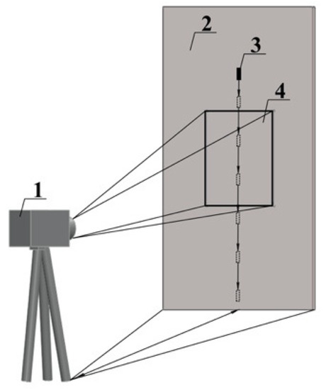
Figure 1.
Schematic of the experiment: 1—IR camera, 2—paper screen, 3—particle, 4—detection frame.
When recording flying particles, their trajectory tends to deviate from the focusing zone of the thermal imaging camera. In order to evaluate the error in determining the particle size, the following test was performed: An object with known geometric dimensions (1396 mm2) was located at a distance of 2.2 m opposite the JADE J530SB, and the camera was focused. Following this, the object was moved 1 m both forward and backward from the focal length with a step of 0.1 m. The set of images was then analyzed using a detector and the errors in the geometric dimensions of the object were calculated, dependent on the distance from the focal length.
Creation of an annotated video database. An experimental setup was used to produce glowing firebrands. More details about this setup can be sourced within the work by [30]. Both a video camera and the JADE J530SB IR camera were used to record firebrands (Figure 2). The distance from the thermal imaging camera to the central plane of the output of the generator was 2.2 m (focus distance). The detection area (frame size) was 0.42(W) × 0.32(H) m and the pixel size was 1.32 × 1.32 mm. The experiments showed that flying particles were recorded with a thermal imaging camera at a distance of ±0.3 m from the focusing zone.
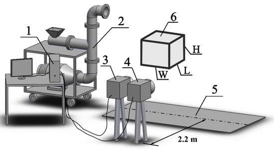
Figure 2.
Experimental setup: 1—data recording system, 2—generator of burning firebrands, 3—IR camera, 4—video camera; 5—test site; 6—detection volume.
Natural particles (pine bark and twigs) and wood pellets were used as firebrands (Figure 3).
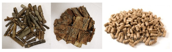
Figure 3.
Firebrand samples.
The size of the particles was selected in accordance with the data of field experiments [17,18,19]. Bark particles were made of pine bark (Pinus sibirica) with sides 10 ± 2, 15 ± 2, 20 ± 2, 25 ± 2, 30 ± 2 mm, and 4–5 mm in thickness. Pine twig particles were 4–6 mm in diameter and had a length of 40 ± 2 and 60 ± 2 mm. The diameter of pine wood pellets was 6–8 ± 1 mm and the length of granules varied from 20 ± 5 to 30 ± 5 mm. The loading mass of the firebrands in the experiments varied within the range of 50–800 g.
2.4. Particle Area and Temperature Measurements
The detection area recorded by the detector contained all pixels, both belonging to the particles and the background (boundary pixels). A threshold value was also used to exclude background pixels. The threshold value for each detection was found as the average value between the maximum and minimum temperatures. According to the calculated threshold value, pixels that held temperatures below the threshold value were eliminated. The result was a set of sizes for each particle in the sequence of frames. The final particle size was then determined as the median value over the entire track. Preliminary tests have shown that the median and threshold values can be used to determine the areas of particles with the most accuracy. The particle temperature was determined from the hottest pixel among all particle detections.
3. Results and Discussion
3.1. Graphical User Interface (GUI) and Video Annotation
The developed GUI (Figure 4a) is used to navigate through video frames (forward, backward, choice of frame with a required number), enlarge the window with frames by a given or arbitrary number of times using the mouse, as well as to select and adjust the parameters of the particle tracking algorithm, run the selected tracker with the given parameters, and finally, to generate the video in AVI format using the tracker.
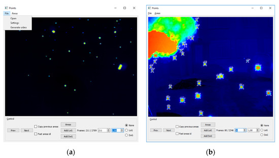
Figure 4.
Developed software: (a) graphical user interface, (b) video annotation.
Checking the accuracy of the developed detectors and trackers requires information on the location and trajectory of the firebrands. Such information is usually obtained manually by marking and numbering all detections and tracks of particles for all frames within the video. This process is typically rather long and time-consuming, as there is a requirement for a large number of frames to be marked to test the algorithms. To accelerate this process, annotation video software was subsequently developed and integrated into the main graphical software interface (Figure 4b). It is used to mark frames in both manual and semi-automatic modes.
Manual marking is carried out by drawing a bounding box around the detection, using a mouse. This rectangle is required to be assigned a particle number (track number). Rectangles can be moved, copied, deleted, and resized. To assist in annotating video, the checkboxes “Copy previous area” and “Fast areas id” are provided in the graphical interface. The first checkbox copies all bounding boxes in the previous frame when moving to the new frame, and the second checkbox automatically numbers the new detections (each new detection will be assigned a number that is larger than the previous number by one).
The interface also includes the “Add LoG” and “Add DoG” buttons, which automatically run available particle tracking algorithms (LoG or DoG) in the current frame. If necessary, the operation of automatic detectors can be corrected manually; for example, deleting or adding a new detection, and correcting the number of the particle track. A video can also be automatically marked using built-in detectors and trackers.
To save and load marked data, a file in the JSON format is used [31], in which the frame number, center coordinates, and the length and width of all bounding boxes marked within it are stored. All detections have unique numbers corresponding to the tracking number.
3.2. Laboratory Experiments
Table 1 shows that an average relative error does not exceed 6% for the 3 m distance or 8% for the 6 m distance. Comparison of different methods to calculate the final projected area of particles among all frames, such as the maximum area, mean area, and the median area, showed that the median area upheld the highest level of accuracy.

Table 1.
Comparison of measured and detected projected median areas of metal particles.
Table 1 demonstrates the way in which pixel size plays an important role in determining particle size. When the distance from the camera to the object increased from 3 to 6 m, the pixel doubled, leading to an increase in the mean relative error by 66% for cylinders and 30% for spheres (the frame frequency was 30 Hz). It is also seen that increasing the frame frequency led to an increase in accuracy. Thus, increasing the frequency from 30 to 190 Hz led to an increase in accuracy by 19–41% for cylinders and 12–14% for spheres. It should be noted that in our study, we used a camera with a 320 × 240 resolution. Using cameras with a higher resolution and frequency will undoubtedly further increase sizing accuracy and recording range.
Analysis of the data obtained after processing the images of the control object at different distances (from the initial position) showed that the relative error of the object area grew almost linearly with increasing distance (Figure 5). In this case, the error grew much faster with the distance of the object from the thermal imaging camera. The maximum error was 33% and 22% when moving away and, respectively, approaching 0.3 m from the focal plane. This difference is most likely related to the features of our thermal imaging camera. It is difficult to draw any conclusions without conducting tests using other thermal imaging cameras.
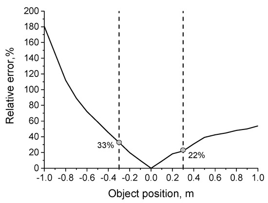
Figure 5.
Changes in the relative error of the object area when moving away from and approaching the focal plane. Negative values on the x-axis correspond to moving the object away from the thermal imaging camera; positive values correspond to approaching the thermal imager, respectively.
3.3. Annotated Video Database
A series of laboratory experiments on the generation and transport of burning firebrands were conducted and 15 videos were recorded. Each video encompasses a set of thermograms/frames (Figure 6) with a duration of 40 to 80 s. Eight time intervals (100 frames each) with a small (5–15, Figure 6a) and medium (16–30, Figure 6b) number of firebrands per frame were selected from the videos recorded (Table 2). The frames with a large number of firebrands (Figure 6c) were excluded from annotation, as it was simply not possible to track firebrands manually.
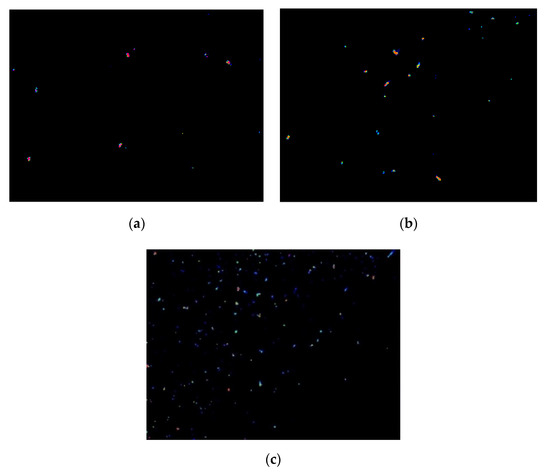
Figure 6.
Example of selected thermograms/frames: (a–c) are the small, medium, and large number of firebrands (pellets), respectively.
Table 2.
Annotated video database.
Table 2, with the characteristics of annotated videos, is given below.
Particles had the following sizes: Pellets–length of 20–30 mm, diameter of 6–8 mm; Twigs—length of 40–60 mm, diameter of 4–6 mm; Bark—length of 10–30 mm, thickness of 4–5 mm. Particle size represents the particles before their burning in the experimental setup.
Each annotated video in Table 2 was separated into two parts. One part was used for the calibration of software (testing detector) and the second part for blind comparison. The calibration process consisted of selecting detector parameters for each type of particle (Table 2, Files 1, 2, 4, 5, 7). Software testing (blind comparison) was performed with selected coefficients (Table 2, Files 3, 6, 8).
3.4. Detector Testing
Using the calibration files (Table 2), the DoG and LoG algorithms were compared and the relative comparison of these two algorithms is presented in Figure 7.
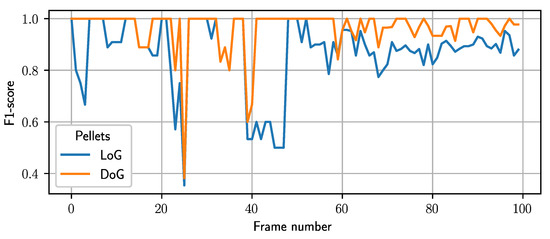
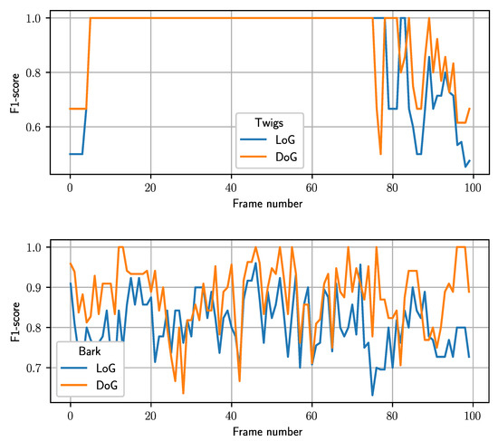
Figure 7.
Relative comparison of LoG and DoG algorithms. High accuracy of F1-score for twigs between the 5th and 75th frames is related to a small number of twigs.
It can be seen that on some frames, the DoG shows excellent performance in comparison with the LoG (e.g., Figure 7, Pellets, Frames 0–12, 39–47) and vice versa (e.g., Figure 7, Twigs, Frames 76–77). Analysis of the frames for pellets showed that the thermal artifacts (thermal reflection from the experimental equipment) were responsible for this. In contrast to the DoG, the LoG detected them as firebrands. The worse performance of the DoG on Frames 76–77 (Twigs) was associated with the detection of flame spots as firebrands. The average value of the F1 score in the studied intervals was 83% for the DoG algorithm and 73% for the LoG algorithm. As such, it can be assumed that the higher DoG accuracy is associated with greater tuning capabilities and fewer false positives of the detector (Figure 8).
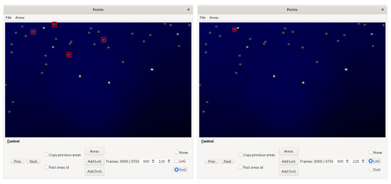
Figure 8.
Comparison of the DoG (left) and LoG (right) detectors for pellets.
Figure 8 shows that the DoG detector discovered more particles than the LoG detector (red rectangles). However, the LoG detected several particles that were not found by the DoG detector (red circle).
The analysis showed that both algorithms can provide the necessary accuracy for the detection of firebrands and are comparable in time and accuracy; however, the DoG algorithm is more easily controlled and implemented. For these reasons, it was selected as the primary detector in the software.
The DoG algorithm was tested using blind tests and one set of parameters for all firebrand types. The results of accuracy testing the DoG detector using the F1 score are presented in Table 3.
Table 3.
The DoG algorithm average accuracy using blind comparison.
It can be seen that blind comparison demonstrated a good agreement for pellets and bark; however, the F1 score reduced almost twice for the twigs. The analysis showed that the combination of parameters that works well for pellets and bark does not give a good F1 score for twigs and vice versa. One of the reasons could be a limited number of annotations and firebrand sizes/shapes used for calibration. A future study will be focused on extending the database.
3.5. Tracker Testing Results
The results of testing the quality of trackers are provided in Table 4. The average values of all tested videos are indicated as the MOTA and MOTP metrics.
Table 4.
Evaluating the quality of tracking algorithms.
The accuracy of the metrics changes from 0 to 100%, where 100% is an absolute coincidence.
The analysis demonstrated the superiority of Hungarian algorithm-based trackers. The MOTA and MOTP metrics have close or higher accuracy for the Hungarian algorithm. MOTP metrics showed similar values for all firebrand types, whilst the MOTA metric showed a higher level of accuracy for pellets and bark. Similar results were also observed for detectors. At this stage of the study, it is not possible to determine the reason behind higher errors in the detection and tracking of twigs. However, the obtained accuracy is in good agreement with the results of other works. For example, multi-object tracking studies [32,33] show a comparable accuracy of the work using the applied tracker algorithms.
A comparison of the number of annotated and tracked firebrands is presented in Figure 9. The results show that the Hungarian algorithm under-tracked the number of firebrands, though showed a level of reasonable accuracy.
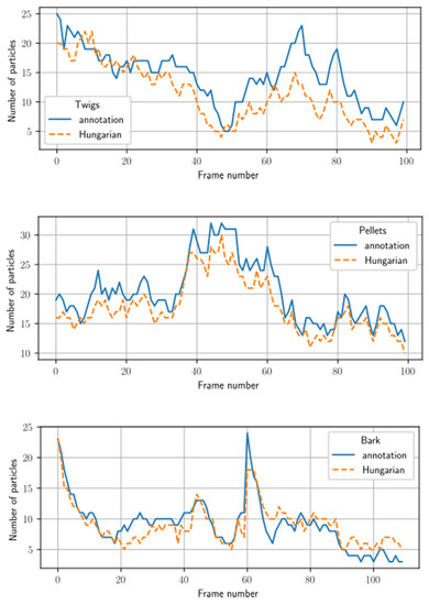
Figure 9.
Blind comparison of the Hungarian algorithm-based tracker. The number of firebrands in each frame shows the number of firebrands tracked from the previous frame.
3.6. Software Application and Future Research
At present, the most effective result has been achieved by utilizing the method based on the DoG detecting algorithm and the Hungarian tracking algorithm. Using the selected algorithms, we calculated a firebrand flux from three experimental videos (Figure 10). The firebrand flux was calculated as a number of particles flying through a square meter per second. Although it was calculated for an area (particles m−2s−1), it is a 3D value, as the software detects particles 0.3 m from a focus distance. The initial mass and number of firebrands for pellets, bark, and twigs were 780 g (933 pieces), 420 g (270 pieces), and 245 g (360 pieces), respectively.
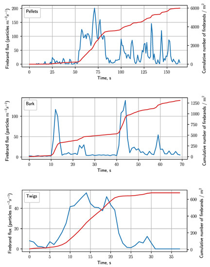
Figure 10.
Firebrand flux during the test period (left axis, blue line) and the total number of firebrands per m2 (right axis, red line).
It can be seen in Figure 10 that the firebrand flux reflects the initial mass of firebrands. It was noted to be the highest for pellets and the smallest for twigs. A firebrand structure may have also held influence over their number. For instance, the cumulative number of firebrands increased by 6.4, 4.8, and 1.9 times compared with the initial number for pellets, bark, and twigs, respectively. Pellets and bark are relatively fragile and fall apart/peel off easily due to high temperatures and airflow, whilst twigs remain intact and mainly reduce in size.
There is potential for using the proposed methodology in field experiments or real fires. However, to utilize it, a high-resolution IR camera or/and a narrow-angle lens should be used. For instance, using a 2° camera lens with a resolution of 320 × 240 pixels will give a 2 cm pixel at a 500 m distance. To maintain reasonable accuracy at this distance, a 3–4 µm IR camera’s spectral range should be used, as this avoids the influence of water vapor and carbon dioxide on the thermal radiation signal. In addition, to avoid the effect of the background, the detection area should be selected above the flaming zone or at some distance from the fire front, where it is protected from flame interference. In our future work, we will test this methodology in a field experiment with a higher resolution camera and a narrower lens field view.
The analysis of testing the detectors and trackers demonstrated that it is problematic to achieve a significant improvement in their accuracy for different shapes and sizes of firebrands. Analysis has also determined that further development of this approach will not significantly improve their accuracy. One of the most promising approaches is the use of convolutional neural networks. This approach holds advantages over traditional (used by us) algorithms, and neural networks can be trained to identify complex relationships between input and output data. In the case of successful training, the network is able to provide the correct result for new data, even if they are incomplete or partially distorted. In the future, it is planned to use convolutional neural networks in order to improve the accuracy and quality of both the detector and the tracker.
3.7. Limitations of the Current Study
IR cameras. The use of infrared cameras for determining the geometric dimensions and temperatures of particles imposes a number of limitations. First, the flying particles are present at a different depth in the frame, often causing inaccuracy in determining the physical dimensions and temperatures of particles due to their contour blurring. Secondly, IR cameras have a limited field of view and therefore cannot record all flying (generated) particles; for example, when burning a tree or using a firebrand generator.
Firebrand’s generator. During the operation of the firebrand’s generator, in addition to particles, a flame is also produced from its output section. This creates limitations in detecting particles directly from the output section. When working with a firebrand’s generator, it is impossible to establish a strict correspondence between the number of starting and generated particles, as some of the particles that are in the combustion chamber are either destroyed or completely burned out.
Software. In the case of a flame or flaming particles appearing in the frame, the detector may begin to mistakenly identify flame as firebrands. The tracker has a limit on the number of tracked particles, so when the number of particles is more than 100 in a frame, the tracker will begin to incorrectly match particles between frames. Additional accuracy problems arise if a particle is split into several particles during flight or when the particle speed is high and the frame rate is low. In addition, for a large detection area and a large number of firebrands, firebrand overlapping will affect the accuracy of the tracker.
All issues outlined above impose restrictions on the use of the proposed approach in field conditions. Nevertheless, it allows the desired characteristics of firebrands to be obtained under laboratory conditions with sufficient accuracy.
4. Conclusions
A series of laboratory experiments were conducted using a firebrand generation experimental setup for the purpose of testing and verifying the developed software. To detect firebrands on the thermograms, the Laplacian of Gaussian (LoG) and the Difference of Gaussian (DoG) algorithms were tested. To evaluate the accuracy of these detectors, an original approach applying the F1 score metric was used. The analysis showed that both metrics can provide the necessary accuracy for the detection of firebrands and are comparable in time and accuracy, however, the DoG algorithm is easier to control and implement. Different firebrand tracking algorithms have been developed and tested. In particular, a Hungarian algorithm-based tracker (the Kuhn–Munkres algorithm) that is designed to track the movement of detection between frames with a higher accuracy was implemented. The analysis of the MOTA and MOTP metrics showed that the Hungarian algorithm-based tracker tracked the movement of firebrands more precisely. Further development of detection and tracking algorithms whilst utilizing the current approach will not significantly improve their accuracy. Therefore, future work will be focused on developing convolutional neural networks.
The results obtained demonstrated that the proposed software allows the desired characteristics of the generation and transport of firebrands to be obtained with reasonable accuracy. Further advances in thermal imaging camera technologies, such as resolution and frequency, are expected to significantly improve accuracy. Firebrand detection and tracking software can be used to improve physics-based and operational fire behavior models, which in turn will significantly increase decision-makers’ ability to evaluate risks during wildland and prescribed fires.
Author Contributions
Conceptualization, A.F.; methodology, S.P., D.K., V.R. and A.F.; formal analysis, S.P., D.K. and A.F.; investigation, S.P., D.K., V.R. and M.A.; writing—original draft preparation, A.F.; writing—review and editing, S.P., D.K., M.A. and A.F.; visualization, S.P., D.K. and M.A. All authors have read and agreed to the published version of the manuscript.
Funding
This work was supported by the Russian Foundation for Basic Research (project #18-07-00548), the Tomsk State University Academic D.I. Mendeleev Fund Program, the State Budget (project II.10.3.8), the Bushfire and Natural Hazard Cooperative Research Centre, and the Program of Increasing the International Competitiveness of the Tomsk State University for 2013–2020.
Acknowledgments
The authors appreciate the assistance from Zakharov O., Perminov V., Martynov P., Golubnichy E., and Orlov K. from the Tomsk State University.
Conflicts of Interest
The authors declare no conflict of interest. The founding sponsors had no role in the design of the study; in the collection, analyses, or interpretation of data; in the writing of the manuscript, and in the decision to publish the results.
References
- Valkó, O.; Török, P.; Deák, B.; Tóthmérész, B. Review: Prospects and limitations of prescribed burning as a management tool in European grasslands. Basic Appl. Ecol. 2014, 15, 26–33. [Google Scholar] [CrossRef]
- Corona, P.; Ascoli, D.; Barbati, A.; Bovio, G.; Colangelo, G.; Elia, M.; Garfì, V.; Iovino, F.; Lafortezza, R.; Leone, V.; et al. Integrated forest management to prevent wildfires under mediterranean environments. Ann. Silvic. Res. 2015, 39, 1–22. [Google Scholar]
- Dupéy, L.N.; Smith, J.W. An Integrative Review of Empirical Research on Perceptions and Behaviors Related to Prescribed Burning and Wildfire in the United States. Environ. Manag. 2018, 61, 1002–1018. [Google Scholar] [CrossRef] [PubMed]
- Leavesley, A.; Wouters, M.; Thornton, R. Prescribed Burning in Australasia: The Science Practice and Politics of Burning the Bush; Australasian Fire and Emergency Service Authorities Council Limited: Melbourne, Australia, 2020. [Google Scholar]
- Morgan, G.W.; Tolhurst, K.G.; Poynter, M.W.; Cooper, N.; McGuffog, T.; Ryan, R.; Wouters, M.A.; Stephens, N.; Black, P.; Sheehan, D.; et al. Prescribed burning in south-eastern Australia: History and future directions. Aust. For. 2020, 83, 4–28. [Google Scholar] [CrossRef]
- Black, A.E.; Hayes, P.; Strickland, R. Organizational Learning from Prescribed Fire Escapes: A Review of Developments over the Last 10 Years in the USA and Australia. Curr. For. Rep. 2020, 6, 41–59. [Google Scholar] [CrossRef]
- Cruz, M.G.; Sullivan, A.L.; Gould, J.S.; Sims, N.C.; Bannister, A.J.; Hollis, J.J.; Hurley, R.J. Anatomy of a catastrophic wildfire: The Black Saturday Kilmore East fire in Victoria, Australia. For. Ecol. Manag. 2012, 284, 269–285. [Google Scholar] [CrossRef]
- Tarifa, C.S.; Notario, P.P.D.; Moreno, F.G. On the flight paths and lifetimes of burning particles of wood. Symp. Combust. 1965, 10, 1021–1037. [Google Scholar] [CrossRef]
- Albini, F.A. Spot Fire Distance from Burning Trees—A Predictive Model; No. General Technical Report INT-GTR-56; USDA Forest Service: Ogden, UT, USA, 1979.
- Albini, F.A. Transport of firebrands by line thermalst. Combust. Sci. Technol. 1983, 32, 277–288. [Google Scholar] [CrossRef]
- Tse, S.D.; Fernandez-Pello, A.C. On the flight paths of metal particles and embers generated by power lines in high winds—A potential source of wildland fires. Fire Saf. J. 1998, 30, 333–356. [Google Scholar] [CrossRef]
- Manzello, S.L.; Suzuki, S. Exposing Decking Assemblies to Continuous Wind-Driven Firebrand Showers. Fire Saf. Sci. 2014, 11, 1339–1352. [Google Scholar] [CrossRef][Green Version]
- Suzuki, S.; Manzello, S.L. Characteristics of Firebrands Collected from Actual Urban Fires. Fire Technol. 2018, 54, 1533–1546. [Google Scholar] [CrossRef] [PubMed]
- Halofsky, J.E.; Peterson, D.L.; Harvey, B.J. Changing wildfire, changing forests: The effects of climate change on fire regimes and vegetation in the Pacific Northwest, USA. Fire Ecol. 2020, 16, 4. [Google Scholar] [CrossRef]
- Radeloff, V.C.; Helmers, D.P.; Kramer, H.A.; Mockrin, M.H.; Alexandre, P.M.; Bar-Massada, A.; Butsic, V.; Hawbaker, T.J.; Martinuzzi, S.; Syphard, A.D.; et al. Rapid growth of the US wildland-urban interface raises wildfire risk. Proc. Natl. Acad. Sci. USA 2018, 115, 3314. [Google Scholar] [CrossRef] [PubMed]
- El Houssami, M.; Mueller, E.; Filkov, A.; Thomas, J.C.; Skowronski, N.; Gallagher, M.R.; Clark, K.; Kremens, R.; Simeoni, A. Experimental Procedures Characterising Firebrand Generation in Wildland Fires. Fire Technol. 2016, 52, 731–751. [Google Scholar] [CrossRef]
- Filkov, A.; Prohanov, S.; Mueller, E.; Kasymov, D.; Martynov, P.; Houssami, M.E.; Thomas, J.; Skowronski, N.; Butler, B.; Gallagher, M.; et al. Investigation of firebrand production during prescribed fires conducted in a pine forest. Proc. Combust. Inst. 2017, 36, 3263–3270. [Google Scholar] [CrossRef]
- Thomas, J.C.; Mueller, E.V.; Santamaria, S.; Gallagher, M.; El Houssami, M.; Filkov, A.; Clark, K.; Skowronski, N.; Hadden, R.M.; Mell, W.; et al. Investigation of firebrand generation from an experimental fire: Development of a reliable data collection methodology. Fire Saf. J. 2017, 91, 864–871. [Google Scholar] [CrossRef]
- Caton-Kerr, S.E.; Tohidi, A.; Gollner, M.J. Firebrand Generation from Thermally-Degraded Cylindrical Wooden Dowels. Front. Mech. Eng. 2019, 5, 32. [Google Scholar] [CrossRef]
- Hedayati, F.; Bahrani, B.; Zhou, A.; Quarles, S.L.; Gorham, D.J. A Framework to Facilitate Firebrand Characterization. Front. Mech. Eng. 2019, 5, 43. [Google Scholar] [CrossRef]
- Liu, K.; Liu, D. Particle tracking velocimetry and flame front detection techniques on commercial aircraft debris striking events. J. Vis. 2019, 22, 783–794. [Google Scholar] [CrossRef]
- Liu, Y.; Urban, J.L.; Xu, C.; Fernandez-Pello, C. Temperature and Motion Tracking of Metal Spark Sprays. Fire Technol. 2019, 55, 2143–2169. [Google Scholar] [CrossRef]
- Bouvet, N.; Link, E.D.; Fink, S.A. Development of a New Approach to Characterize Firebrand Showers during Wildland-Urban Interface (WUI) Fires: A Step towards High-Fidelity Measurements in Three Dimensions; No. Technical Note; NIST: Gaithersburg, MD, USA, 2020.
- Filkov, A.; Prohanov, S. Particle Tracking and Detection Software for Firebrands Characterization in Wildland Fires. Fire Technol. 2019, 55, 817–836. [Google Scholar] [CrossRef]
- Guttag, J.V. Introduction to Computation and Programming Using Python; MIT Press: Cambridge, MA, USA, 2013. [Google Scholar]
- Hand, D.; Christen, P. A note on using the F-measure for evaluating record linkage algorithms. Stat. Comput. 2018, 28, 539–547. [Google Scholar] [CrossRef]
- Knuth, D.E. The Art of Computer Programming, 3rd ed.; Fundamental Algorithms; Addison Wesley Longman Publishing Co., Inc.: Boston, MA, USA, 1997; Volume 1. [Google Scholar]
- Munkres, J. Algorithms for the Assignment and Transportation Problems. J. Soc. Ind. Appl. Math. 1957, 5, 32–38. [Google Scholar] [CrossRef]
- Bernardin, K.; Stiefelhagen, R. Evaluating Multiple Object Tracking Performance: The CLEAR MOT Metrics. EURASIP J. Image Video Process. 2008, 2008, 246309. [Google Scholar] [CrossRef]
- Kasymov, D.P.P.V.V.; Filkov, A.I.; Agafontsev, A.M.; Reyno, V.V.; Gordeev, E.V. Generator of Flaming and Glowing Firebrands; FIPS: Moscow, Russia, 2017; p. 183063. [Google Scholar]
- Introducing JSON. Available online: https://www.json.org/ (accessed on 31 August 2020).
- Hua, W.; Mu, D.; Zheng, Z.; Guo, D. Online multi-person tracking assist by high-performance detection. J. Supercomput. 2017, 76, 4076–4094. [Google Scholar] [CrossRef]
- Rahul, M.V.; Ambareesh, R.; Shobha, G. Siamese Network for Underwater Multiple Object Tracking. In Proceedings of the 9th International Conference on Machine Learning and Computing, Singapore, 24–26 February 2017; pp. 511–516. [Google Scholar]
Publisher’s Note: MDPI stays neutral with regard to jurisdictional claims in published maps and institutional affiliations. |
© 2020 by the authors. Licensee MDPI, Basel, Switzerland. This article is an open access article distributed under the terms and conditions of the Creative Commons Attribution (CC BY) license (http://creativecommons.org/licenses/by/4.0/).