Predicting Emission Source Terms in a Reduced-Order Fire Spread Model—Part 1: Particulate Emissions

 , , , and
Abstract

1. Introduction
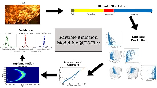
2. Model Development
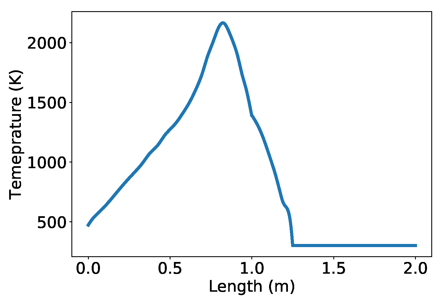
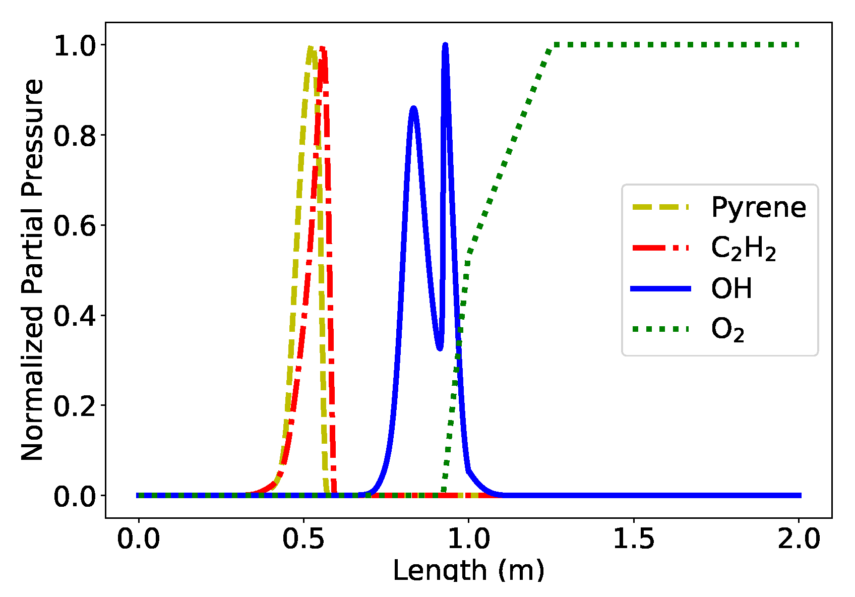
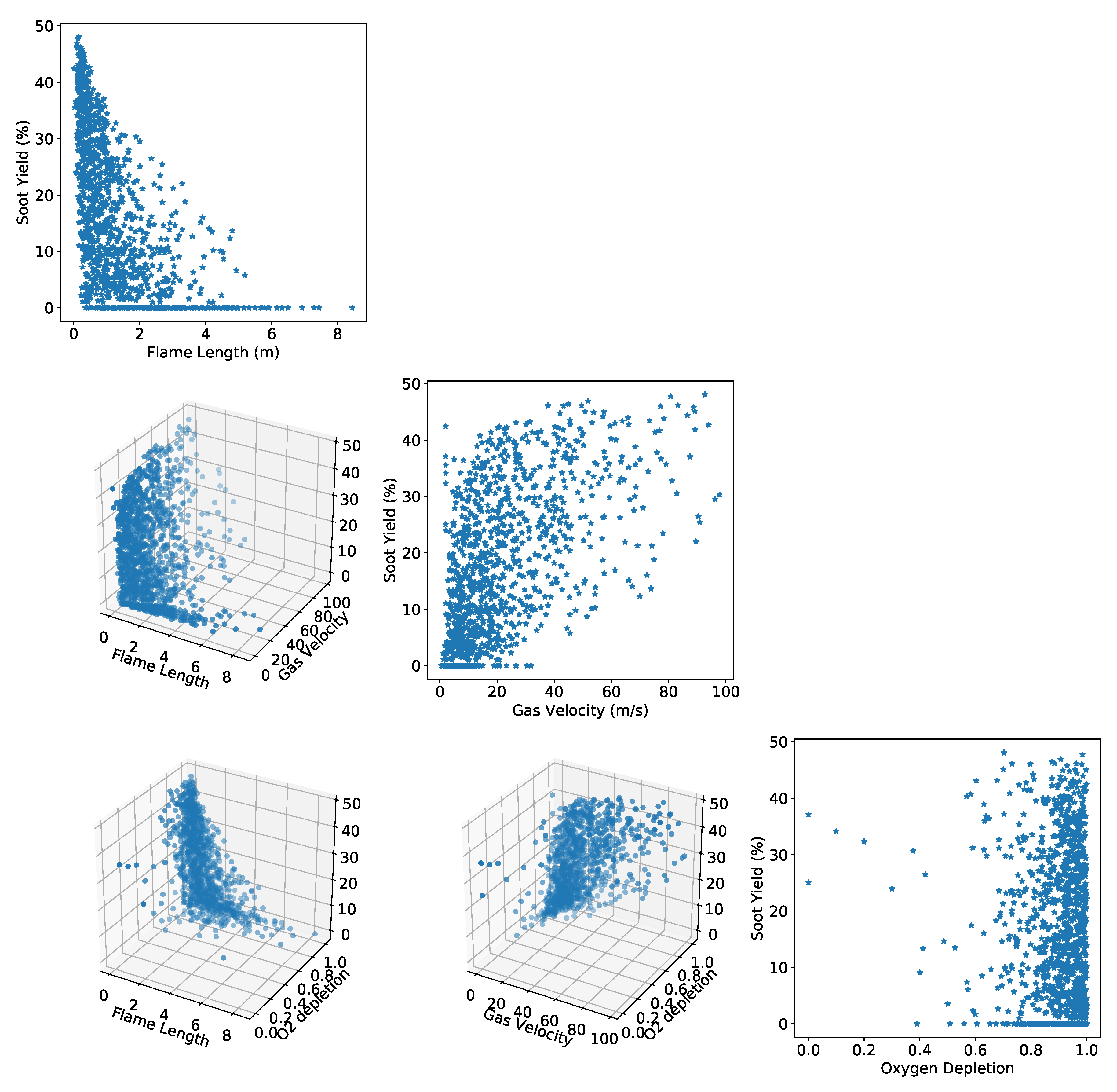
2.1. Flamelet Simulation
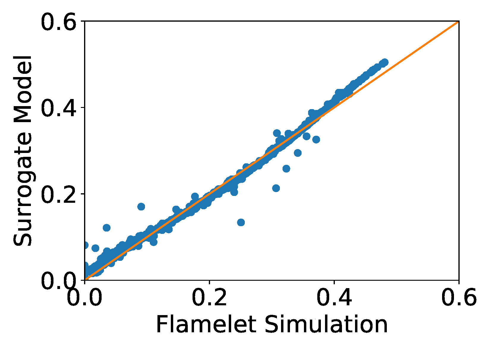
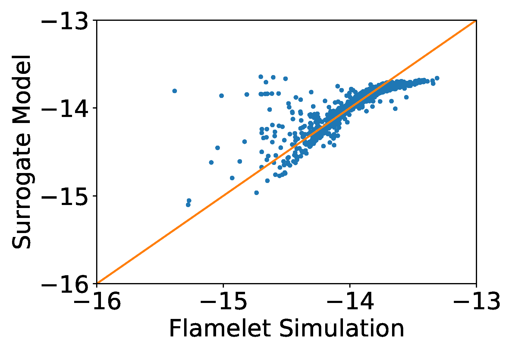
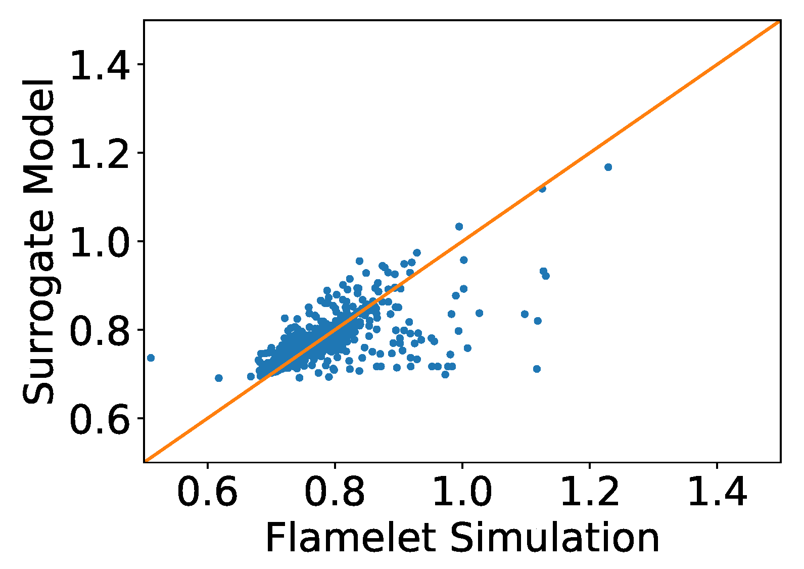
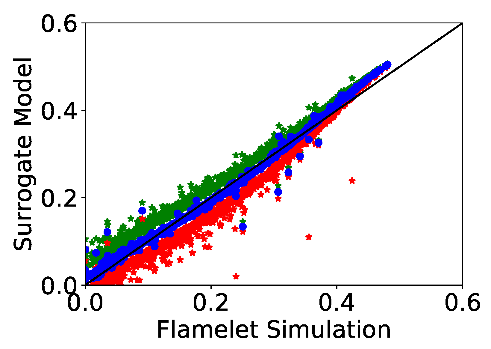
2.2. Surrogate Model Development
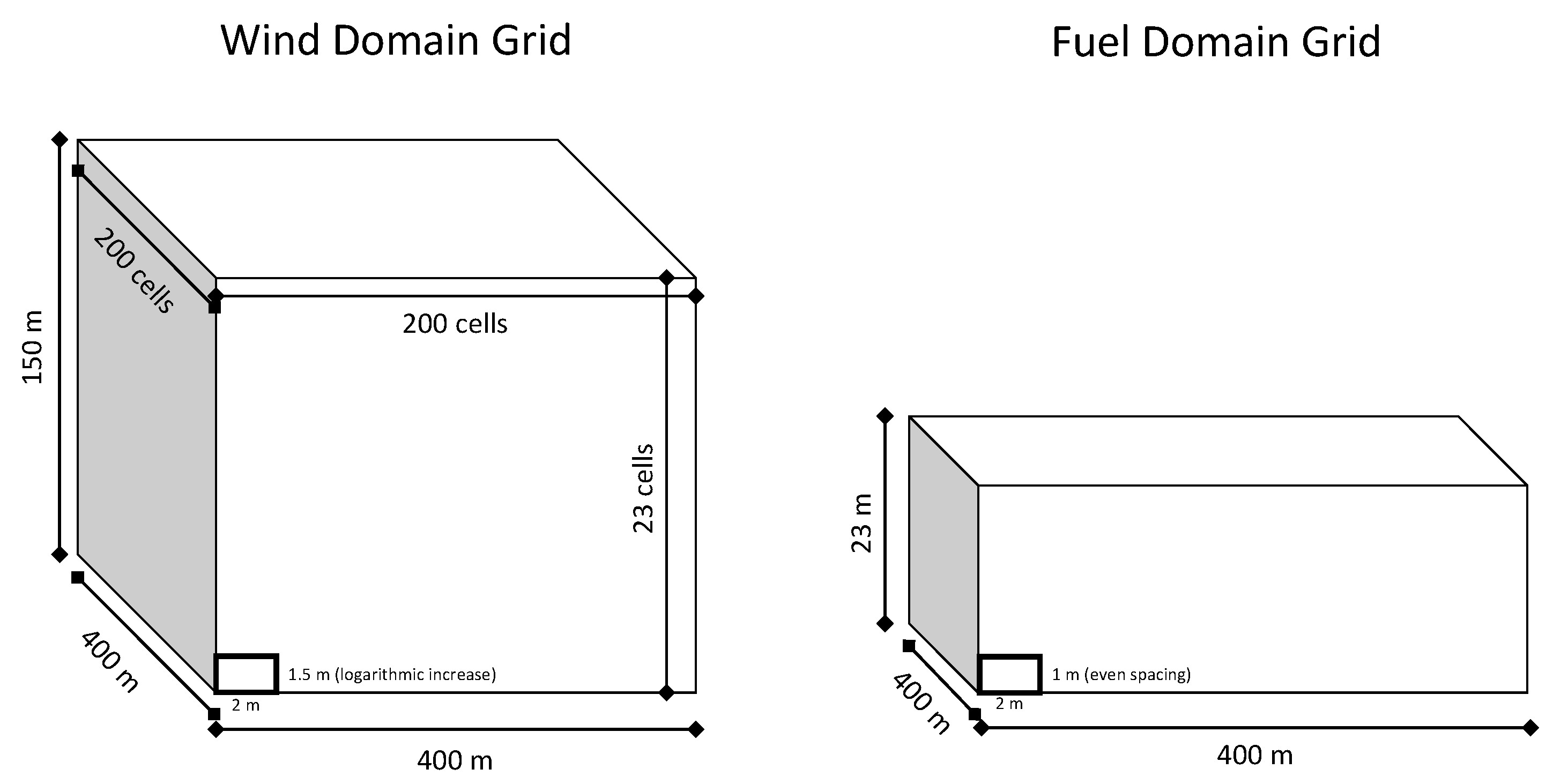
3. Simulations
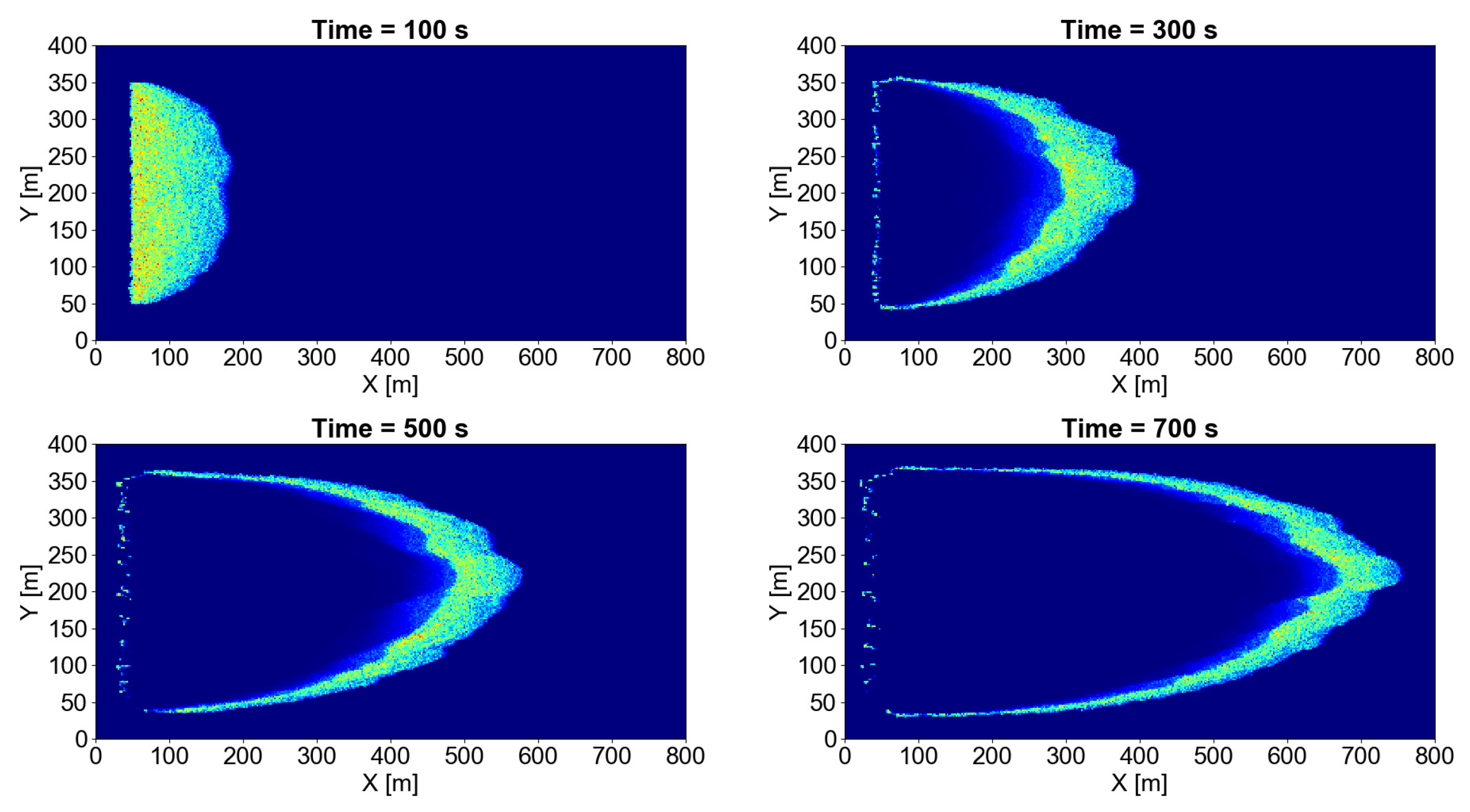
3.1. QUIC-Fire
3.2. Implementations
4. Results and Discussion
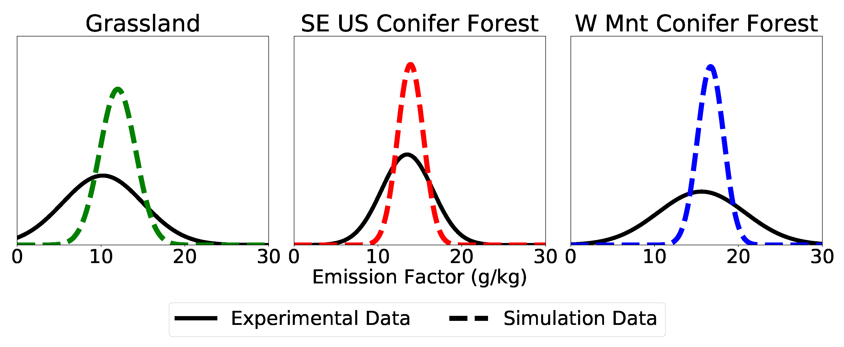
4.1. Emission Factors
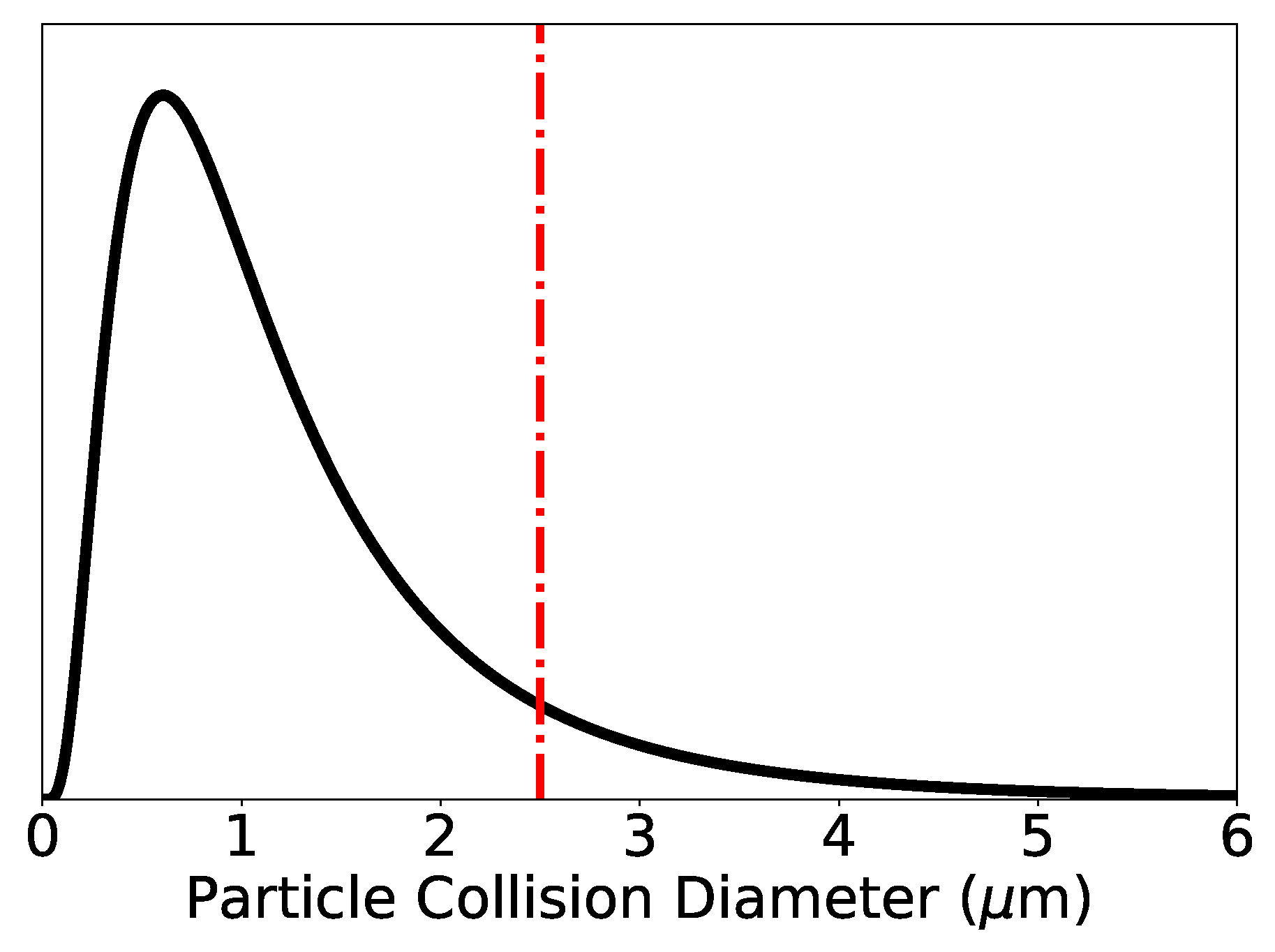
4.2. Particle Size Distributions
5. Conclusions
Author Contributions
Funding
Conflicts of Interest
Appendix A. Uncertainty Quantification
Appendix A.1

References
- Linn, R.R.; Sieg, C.H.; Hoffman, C.M.; Winterkamp, J.L.; Mcmillin, J.D. Modeling wind fields and fire propagation following bark beetle outbreaks in spatially-heterogeneous pinyon-juniper woodland fuel complexes. Agric. For. Meteorol. 2013, 173, 139–153. [Google Scholar] [CrossRef]
- Rim, C.B.; Om, K.C.; Ren, G.; Kim, S.S.; Kim, H.C.; Kang-Chol, O. Establishment of a wildfire forecasting system based on coupled weather–Wildfire modeling. Appl. Geogr. 2018, 90, 224–228. [Google Scholar] [CrossRef]
- Linteris, G.T.; Gewuerz, L.; McGrattan, K.B.; Forney, G. Modeling Solid Sample Burning with FDS; Technical Report; National Institute of Standards and Technology: Gaithersburg, MD, USA, 2004. [CrossRef]
- Linn, R.R.; Goodrick, S.; Brambilla, S.; Brown, M.J.; Middleton, R.; O’Brien, J.J.; Hiers, J.K. QUIC-Fire: A fast running simulation tool for prescribed fire planning. Envion. Model. Softw. 2020. [Google Scholar] [CrossRef]
- Whitby, E.R.; McMurry, P.H. Modal Aerosol Dynamics Modeling. Aerosol Sci. Technol. 1997, 27, 673–688. [Google Scholar] [CrossRef]
- Urbanski, S.P. Wildland fire emissions, carbon, and climate: Emission factors. For. Ecol. Manag. 2014, 317, 51–60. [Google Scholar] [CrossRef]
- Akagi, S.K.; Yokelson, R.J.; Wiedinmyer, C.; Alvarado, M.J.; Reid, J.S.; Karl, T.; Crounse, J.D.; Wennberg, P.O. Emission factors for open and domestic biomass burning for use in atmospheric models. Atmos. Chem. Phys. 2011, 11, 4039–4072. [Google Scholar] [CrossRef]
- Hays, M.D.; Geron, C.D.; Linna, K.J.; Smith, N.D.; Schauer, J.J. Speciation of gas-phase and fine particle emissions from burning of foliar fuels. Environ. Sci. Technol. 2002. [Google Scholar] [CrossRef]
- Alexandridis, A.; Vakalis, D.; Siettos, C.; Bafas, G. A cellular automata model for forest fire spread prediction: The case of the wildfire that swept through Spetses Island in 1990. Appl. Math. Comput. 2008, 204, 191–201. [Google Scholar] [CrossRef]
- Almeida, R.M.; Macau, E.E.N. Stochastic cellular automata model for wildland fire spread dynamics. J. Phys. Conf. Ser. 2011, 285. [Google Scholar] [CrossRef]
- Achtemeier, G.L. Field validation of a free-agent cellular automata model of fire spread with fire-atmosphere coupling. Int. J. Wildland Fire 2013, 22, 148–156. [Google Scholar] [CrossRef]
- Robinson, M.S.; Chavez, J.; Velazquez, S.; Jayanty, R.K.M. Chemical Speciation of PM2.5 Collected during Prescribed Fires of the Coconino National Forest near. J. Air Waste Manag. Assoc. 2004, 54, 1112–1123. [Google Scholar] [CrossRef] [PubMed]
- Bilger, R. The Structure of Diffusion Flames. Combust. Sci. Technol. 1976, 13, 155–170. [Google Scholar] [CrossRef]
- Josephson, A.J.; Linn, R.R.; Lignell, D.O. Modeling soot formation from solid complex fuels. Combust. Flame 2018, 196, 265–283. [Google Scholar] [CrossRef]
- Monson, E.I.; Lignell, D.O.; Finney, M.A.; Werner, C.; Jozefik, Z.; Kerstein, A.R.; Hintze, R.S. Simulation of Ethylene Wall Fires Using the Spatially-Evolving One-Dimensional Turbulence Model. Fire Technol. 2016, 52, 167–196. [Google Scholar] [CrossRef]
- Lignell, D.O.; Chen, J.H.; Smith, P.J. Three-dimensional direct numerical simulation of soot formation and transport in a temporally evolving nonpremixed ethylene jet flame. Combust. Flame 2008, 155, 316–333. [Google Scholar] [CrossRef]
- Biermann, C.J. Handbook of Pulping and Papermaking, 2nd ed.; Academic Press: San Diego, CA, USA, 1996. [Google Scholar] [CrossRef]
- Appel, J.; Bockhorn, H.; Frenklach, M. Kinetic Modeling of Soot Formation with Detailed Chemistry and Physics: Laminar Premixed Flames of C2 Hydrocarbons. Combust. Flame 2000, 121, 122–136. [Google Scholar] [CrossRef]
- Lewis, A.D.; Fletcher, T.H. Prediction of Sawdust Pyrolysis Yields from a Flat-Flame Burner Using the CPD Model. Energy Fuels 2013, 27, 942–953. [Google Scholar] [CrossRef]
- Frenklach, M. Method of moments with interpolative closure. Chem. Eng. Sci. 2002, 57, 2229–2239. [Google Scholar] [CrossRef]
- Hosseini, S.; Li, Q.; Cocker, D.R.I.; Weise, D.R.; Miller, A.; Shrivastava, M.; Miller, J.W.; Mahalingam, S.; Princevac, M.; Jung, H.J. Particle size distributions from laboratory-scale biomass fires using fast response instruments. Atmos. Chem. Phys. 2010, 10, 8065–8076. [Google Scholar] [CrossRef]
- Brown, M.J. Quick Urban and Industrial Complex (QUIC) CBR Plume Modeling System: Validation-Study Document; Technical Report; Los Alamos National Laboratory: Los Alamos, NM, USA, 2018. [Google Scholar]
- Clements, C.B.; Seto, D. Observations of Fire-Atmosphere Interactions and Near-Surface Heat Transport on a Slope. Bound.-Layer Meteorol. 2015, 154, 409–426. [Google Scholar] [CrossRef]
- Morton, B.R.; Taylor, G.I.; Turner, J.S. Turbulent gravitational convection from maintained and instantaneous sources. Proc. R. Soc. Lond. A Math. Phys. Sci. 1956, 234, 1–23. [Google Scholar] [CrossRef]
- Briggs, G.A. Plume Rise Predictions. In Lectures on Air Pollution and Environmental Impact Analyses; American Meteorological Society: Boston, MA, USA, 1982; pp. 59–111. [Google Scholar] [CrossRef]
- Weil, J.C. Plume Rise. In Lectures on Air Pollution Modeling; American Meteorological Society: Boston, MA, USA, 1988; pp. 119–166. [Google Scholar] [CrossRef]
- Lai, A.C.H.; Lee, J.H.W. Dynamic interaction of multiple buoyant jets. J. Fluid Mech. 2012, 708, 539. [Google Scholar] [CrossRef]
- Linn, R.R.; Cunningham, P. Numerical simulations of grass fires using a coupled atmosphere-fire model: Basic fire behavior and dependence on wind speed. J. Geophys. Res. 2005, 110. [Google Scholar] [CrossRef]
- Urbanski, S.P.; Hao, W.M.; Baker, S. Chemical Composition of Wildland Fire Emissions. In Developments in Environmental Science; Elsevier: Amsterdam, The Netherlands, 2008; Volume 8, Chapter 4; pp. 79–107. [Google Scholar] [CrossRef]
- Radke, L.F.; Stith, J.L.; Hegg, D.A.; Hobbs, P.V. Airborne Studies of Particles and Gases from Forest Fires. J. Air Pollut. Control Assoc. 2012, 28, 30–34. [Google Scholar] [CrossRef]
- Harris, S.J.; Maricq, M.M. The role of fragmentation in defining the signature size distribution of diesel soot. J. Aerosol Sci. 2002, 33, 935–942. [Google Scholar] [CrossRef]
- Raj, A.; Tayouo, R.; Cha, D.; Li, L.; Ismail, M.A.; Chung, S.H. Thermal fragmentation and deactivation of combustion-generated soot particles. Combust. Flame 2014, 161, 2446–2457. [Google Scholar] [CrossRef]
- Ghiassi, H.; Toth, P.; Jaramillo, I.C.; Lighty, J.S. Soot oxidation-induced fragmentation: Part 1: The relationship between soot nanostructure and oxidation-induced fragmentation. Combust. Flame 2016, 163, 179–187. [Google Scholar] [CrossRef]


| Cellulose | Hardwood | Softwood | ||
|---|---|---|---|---|
| Hemicellulose | Lignin | Hemicellulose | Lignin | |
| 0.46 | 0.06 | 0.00 | 0.21 | 0.27 |
| Fire Class | Wind Speed at 10 m (m/s) | Initial Fireline Length (m) | ||
|---|---|---|---|---|
| Min | Max | Min | Max | |
| Grassland | 2.0 | 12.0 | 25.0 | 275.0 |
| SE US Conifer Forest | 2.0 | 12.0 | 25.0 | 300.0 |
| W Mnt Conifer Forest | 2.0 | 12.0 | 25.0 | 300.0 |
| Ground Fuel Moisture Content (%) | Canopy Fuel Moisture Content (%) | |||
| Min | Max | Min | Max | |
| Grassland | 2 | 12 | — | — |
| SE US Conifer Forest | 2 | 14 | 75 | 150 |
| W Mnt Conifer Forest | 2 | 20 | 65 | 150 |
| Ground Fuel Density (kg/m3) with a Fuel Height of 0.7 m | ||||
| min | max | |||
| Grassland | 2.0 | 12.0 | ||
| SE US Conifer Forest | 1.573 | 1.573 | ||
| W Mnt Conifer Forest | 5.5 | 5.5 | ||
| Fire Class | eμ·10−6 | σ | ||||
|---|---|---|---|---|---|---|
| Mean | Min | Max | Mean | Min | Max | |
| Grassland | 0.992 | 1.043 | 0.905 | 0.708 | 0.700 | 0.722 |
| SE US Conifer Forest | 1.014 | 0.900 | 1.064 | 0.704 | 0.701 | 0.715 |
| W Mnt Conifer Forest | 0.997 | 0.734 | 1.045 | 0.707 | 0.702 | 0.721 |
© 2020 by the authors. Licensee MDPI, Basel, Switzerland. This article is an open access article distributed under the terms and conditions of the Creative Commons Attribution (CC BY) license (http://creativecommons.org/licenses/by/4.0/).
Share and Cite
Josephson, A.J.; Holland, T.M.; Brambilla, S.; Brown, M.J.; Linn, R.R. Predicting Emission Source Terms in a Reduced-Order Fire Spread Model—Part 1: Particulate Emissions. Fire 2020, 3, 4. https://doi.org/10.3390/fire3010004
Josephson AJ, Holland TM, Brambilla S, Brown MJ, Linn RR. Predicting Emission Source Terms in a Reduced-Order Fire Spread Model—Part 1: Particulate Emissions. Fire. 2020; 3(1):4. https://doi.org/10.3390/fire3010004
Chicago/Turabian StyleJosephson, Alexander J., Troy M. Holland, Sara Brambilla, Michael J. Brown, and Rodman R. Linn. 2020. "Predicting Emission Source Terms in a Reduced-Order Fire Spread Model—Part 1: Particulate Emissions" Fire 3, no. 1: 4. https://doi.org/10.3390/fire3010004
APA StyleJosephson, A. J., Holland, T. M., Brambilla, S., Brown, M. J., & Linn, R. R. (2020). Predicting Emission Source Terms in a Reduced-Order Fire Spread Model—Part 1: Particulate Emissions. Fire, 3(1), 4. https://doi.org/10.3390/fire3010004