1. Introduction
Cold atmospheric plasma (CAP) is a unique plasma generated in a glow discharge with a weak ionization level [
1]. CAP is a thermal nonequilibrium plasma with all heavy particles at near room temperature due to the weak elastic collision between electrons and other heavy particles in discharge [
2]. CAP has plenty of reactive species with a relatively low-temperature nature, making it very suitable for treating temperature-sensitive material and, in particular, medical applications [
3,
4].
In plasma medicine, two types of plasma sources have been widely used: dielectric barrier discharge (DBD) and atmospheric pressure plasma jets (APPJs) [
5]. DBD and APPJs share similar physical principles but result in different plasma output configurations [
6]. Both are based on streamer discharge [
7]. DBD creates a large area of plasma composed of dozens of streamers between two parallel electrodes [
8]. In contrast, an APPJ generates a single streamer in each discharge cycle and forms a plasma with a high aspect ratio [
9]. The length of the plasma plume in an APPJ can reach at least 11 cm in some optimized designs [
10]. Such a basic feature positions the APPJ as a powerful tool for treating samples of different sizes, particularly in deep but narrow spaces and samples with small, focused areas requiring treatment [
11].
The size of a plasma plume, particularly the length, is an important physical feature that can be quickly recognized, which is a necessary foundation for realizing future self-adaptive plasma sources [
12]. The framework to realize an intelligent plasma source has been proposed based on modern controlling techniques and machine learning theories [
13,
14]. These novel plasma sources can resist complex environmental changes and retain their stability at an unprecedented level, which may deeply impact the future design and development of CAP sources in plasma medicine [
15].
Here, for the first time, we demonstrated a real–time computer vision (CV) recognition method based on a simple cell phone and PC setup, which can capture the visual image of a plasma plume in an APPJ source and provide plume length information. Based on this modality, we studied the impact of three operational parameters on the plasma plume’s length: the duty cycle of pulse input signals, discharge frequency, and helium flow rate. This study provides a solid foundation for realizing an intelligent, self–adaptable CAP source [
16].
2. Methods and Materials
2.1. APPJ Source
APPJ source was assembled at Micro–propulsion and Nanotechnology Laboratory (MpNL) at the George Washington University.
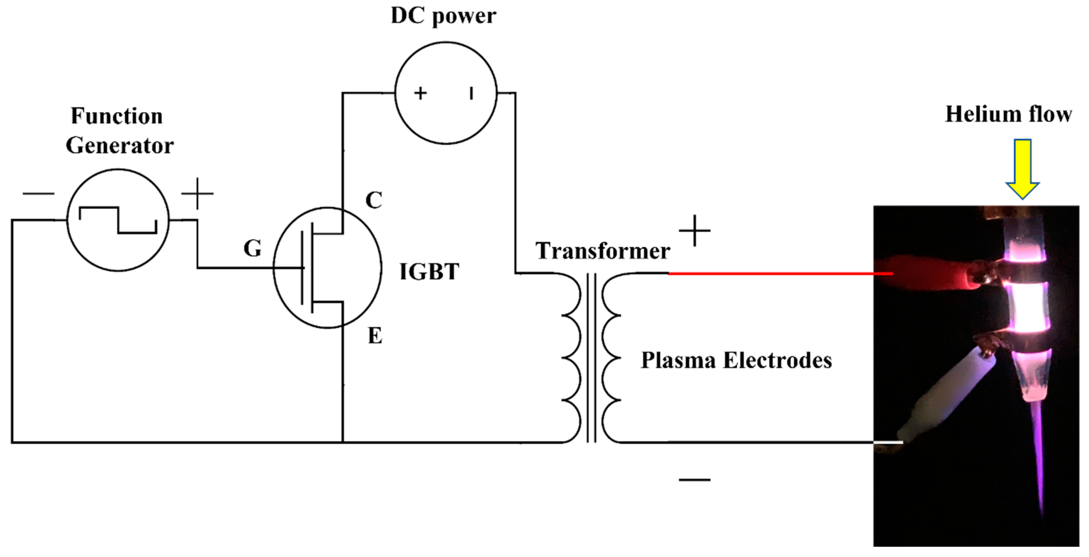
Figure 1 shows the helium gas (99.995% purity, grade 4.5, Roberts Oxygen) flow through a glass tube (diameter of 10 mm). Discharge was triggered by an alternating current between two annulus copper electrodes wrapped around the glass tube. The vertical distance between electrodes varied from 2.1 cm to 9.8 cm. A pulse-shaped wave was used to create the alternating current, and the pulse frequency varied in the kHz range. Input DC power voltages to the transformer were kept much below the 800 V maximum specified by the device, typically between 10–20 V. Duty cycle generally ranged from 20–30%. The ionized gas flowed away from the main discharge area and entered the air to form a violet plasma plume below the nozzle, which had a diameter of 5 mm. A flow meter (Brooks Sho-Rate™) modulated helium flow into the glass tube. Reactive species including reactive oxygen species (ROS) and reactive nitrogen species (RNS) were generated in the plasma plume, which was due to the ionization of oxygen and nitrogen in the air. All experiments were performed under the room temperature (20 °C).
2.2. Computer Vision
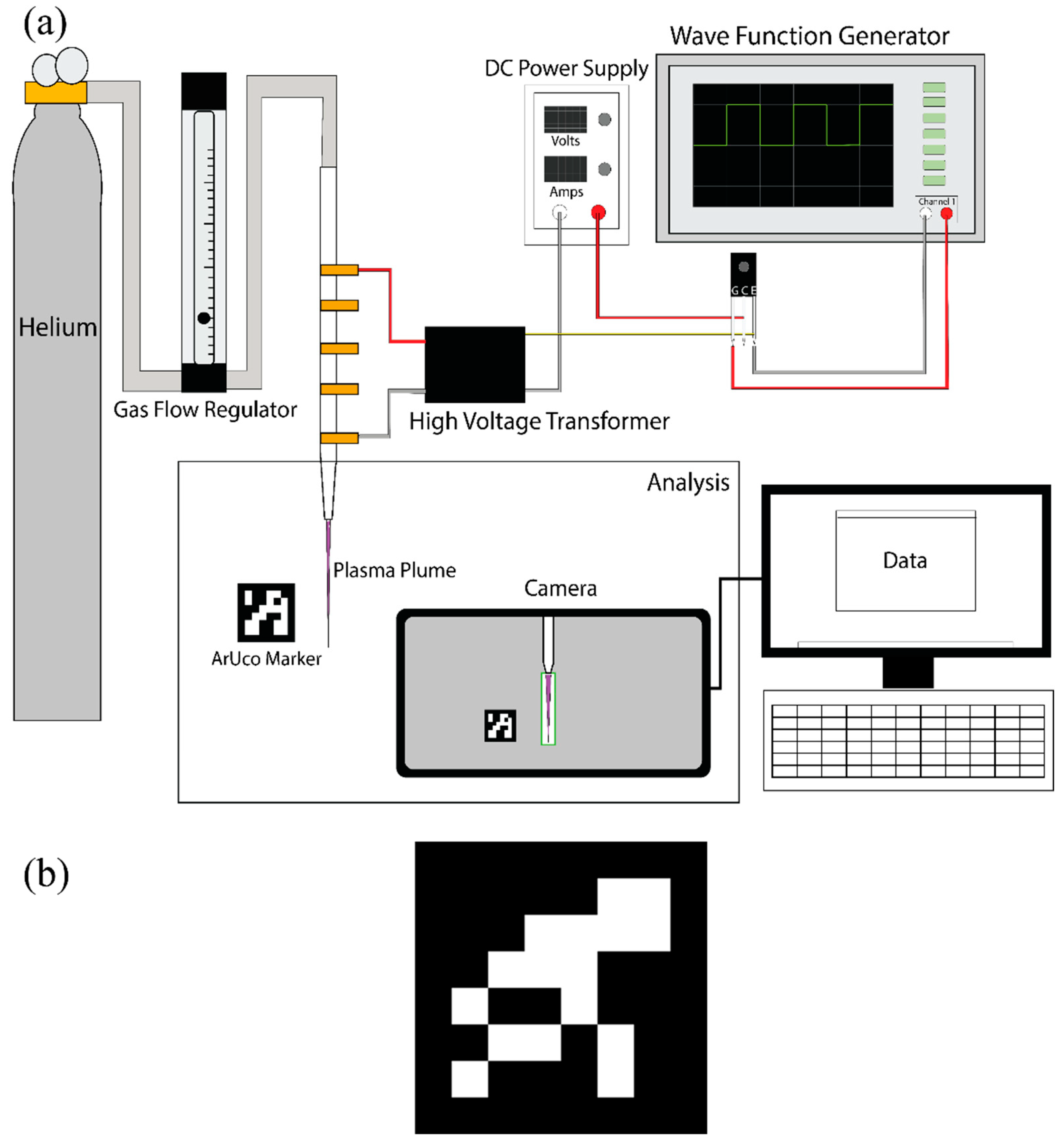
The real-time computer recognition system was schematically illustrated in
Figure 2a. An OpenCV–Python program was used to identify and measure plasma plume lengths in real time from a cell phone (iPhone) video stream. The Python program consisted of 3 main steps: (1) camera calibration, (2) plasma plume identification, and (3) data collection. The workflow was automated using the cv2.waitKey() function from OpenCV-Python. This allowed single keyboard presses to trigger functionality. Important functionality was implemented this way, including calibration, data collection, and printing of HSV values.
The program used ArUco markers to calibrate the camera position before measurements were started (
Figure 2b). The calibration calculation and specific equipment details can also be found in
Supporting Materials.
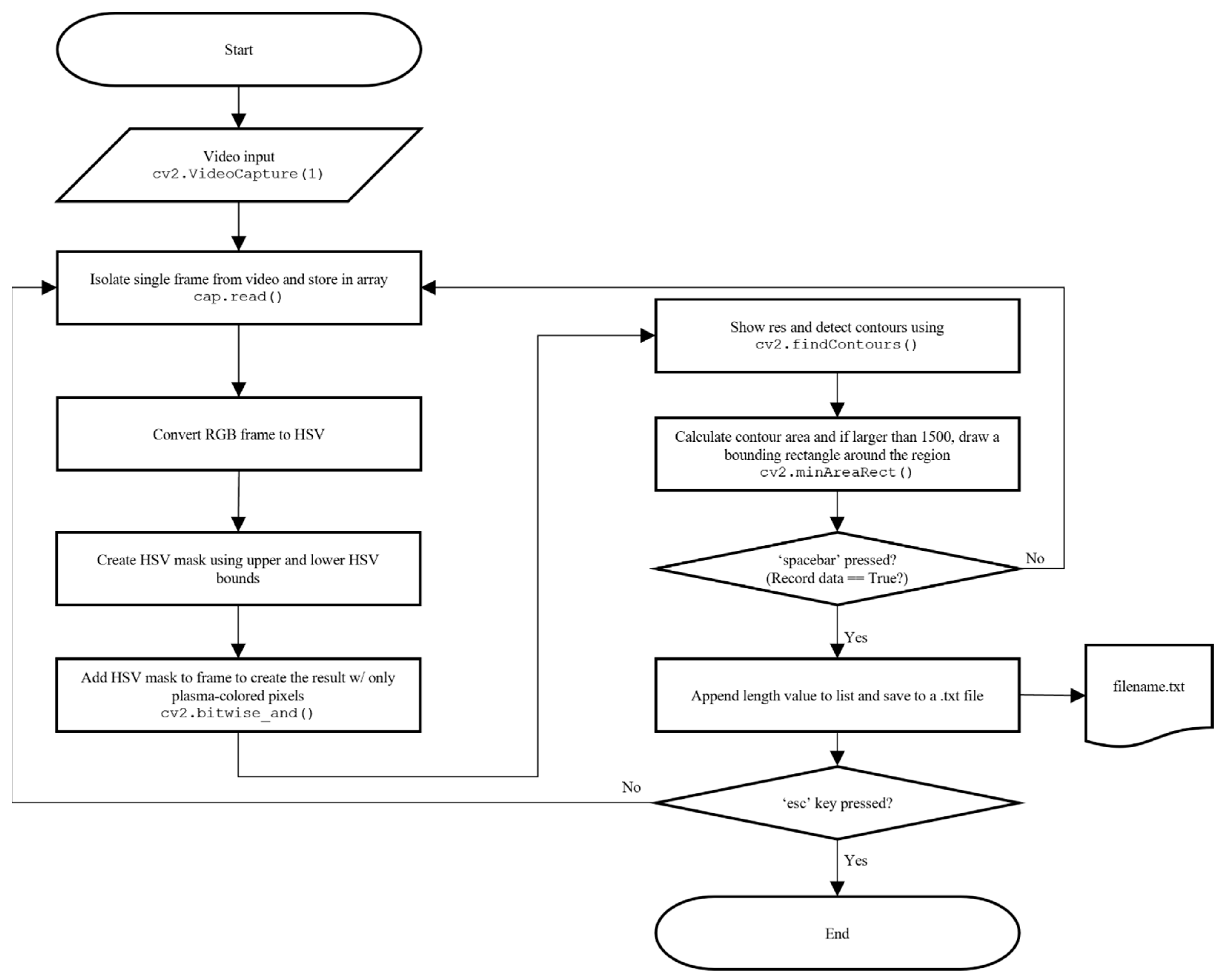
The program recognized plasma plumes by first converting the video frames from red–green–blue (RGB) to HSV. Next, a mask excluded all pixels outside the color bounds, effectively selecting only purple pixels. The plasma plumes were identified by upper and lower hue, saturation, value (HSV). HSV values were printed when the “p” key was pressed. The threshold values could be adjusted during program development with a graphical user interface (GUI) slider window. Exact upper and lower values were determined using the process described in the
Supporting Material during software testing and then held constant during measurements.
The color mask was added with the original video frame to produce a resulting frame containing only the purple plasma regions. Contours were identified using cv2.findContours(). Bounding boxes were drawn around the contours that enclosed a minimum threshold area; the box dimension representing the plume length was selected and saved.
All GUI windows displayed indefinitely until the “esc” key was pressed, which closed all windows and terminated the program. The “spacebar” key press triggered the data collection process. Bounding box dimensions in pixels were converted to metric and the longer of the two dimensions (width or height) was accessed, stored in an array, and then saved to a file. For this project, we collected 100 frames for each experimental measurement. Typically, this took around 10–12 s to collect. After collecting 100 frames, the average and standard deviation were calculated and plotted for different experimental conditions. The program described above can be visualized in a flow chart (
Figure 3). Program source code is included in
Supporting Materials. The “plasma_cv.py” file is the main program that relies on “aruco_calibrate.py” for the calibration function.
3. Results
3.1. Plume Identification
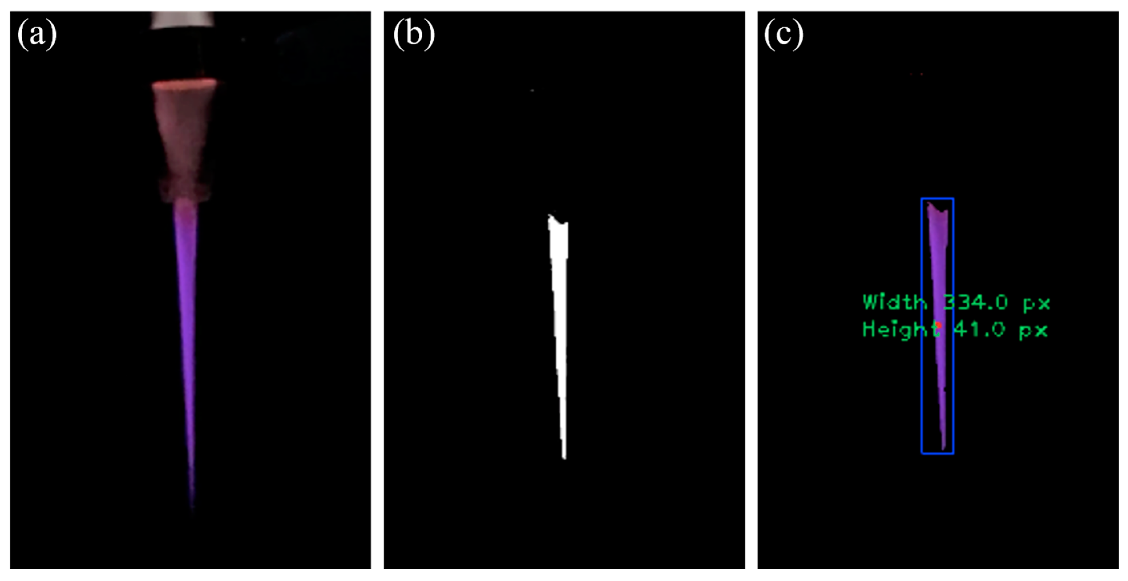
Plasma plumes were successfully identified using our approach. Three GUI windows, shown in
Figure 4, were displayed when the program was running.
Figure 4a showed the “frame” window, which was the raw input to the program.
Figure 4b was the “mask” that was created from the HSV thresholds set during program development. The white pixels had a value of 1, and the black pixels were set to 0. Finally,
Figure 4c is the “result” window because it was the result returned from the additive cv2 operation cv2.bitwise_and().
HSV thresholds were given in
Table 1. Standard HSV value ranges are (0–360°), (0–100%), and (0–100%) for hue, saturation, and value, respectively. For OpenCV, HSV values range from (0–180), (0–255), and (0–255). To determine the upper and lower HSV values for the program to identify the characteristic color of plasma, a sample image of a plasma plume was taken with a camera and inputted to a generic online color picker. The color picker returned standard HSV values and then a simple proportion was used to calculate the OpenCV analog. For example, for a representative image of plasma, the online color picker (
https://redketchup.io/color-picker (accessed on 25 March 2022) returned HSV values approximately (250, 55, and 50) for the plume. Normalizing these to the OpenCV ranges resulted in values close to those shown in
Table 1. Lower limits were slightly extended; this was to better capture the tip of the jet, which is generally less illuminating and saturated, but lower saturation and value limits were not extended enough where the program falsely identified plasma outside the region of interest. Upper ranges for saturation and value were set at a maximum to ensure capture of the bright regions of plasma, which are the most reactive. Hue range was able to be maximized because of the operational parameter of the black background. It is important to note that if the background used was not constant and black, the maximum hue value of the program would likely have to be adjusted.
The bitwise_and() function overlayed the mask on the frame and produced a copy of the raw input with black pixels everywhere except the white region from the mask. This allowed us to quickly find contours in the “result” and calculate pixel dimensions using tight bounding boxes around the area.
3.2. Computer Vision Demonstration
To test the ability of the computer vision plasma recognition program, we performed the following tests of three important operational parameter effects on plasma plume length, including duty cycle, discharge frequency, and gas flow. In all figures, plume length measurements from 100 frames were averaged. This was repeated in three separate trials. Next, averages and standard deviations were calculated from the three trials and plotted. Finally, we interpreted higher standard deviations as larger plasma plume fluctuations. These could be an indication of high turbulence in the flow and more unpredictable plasma output.
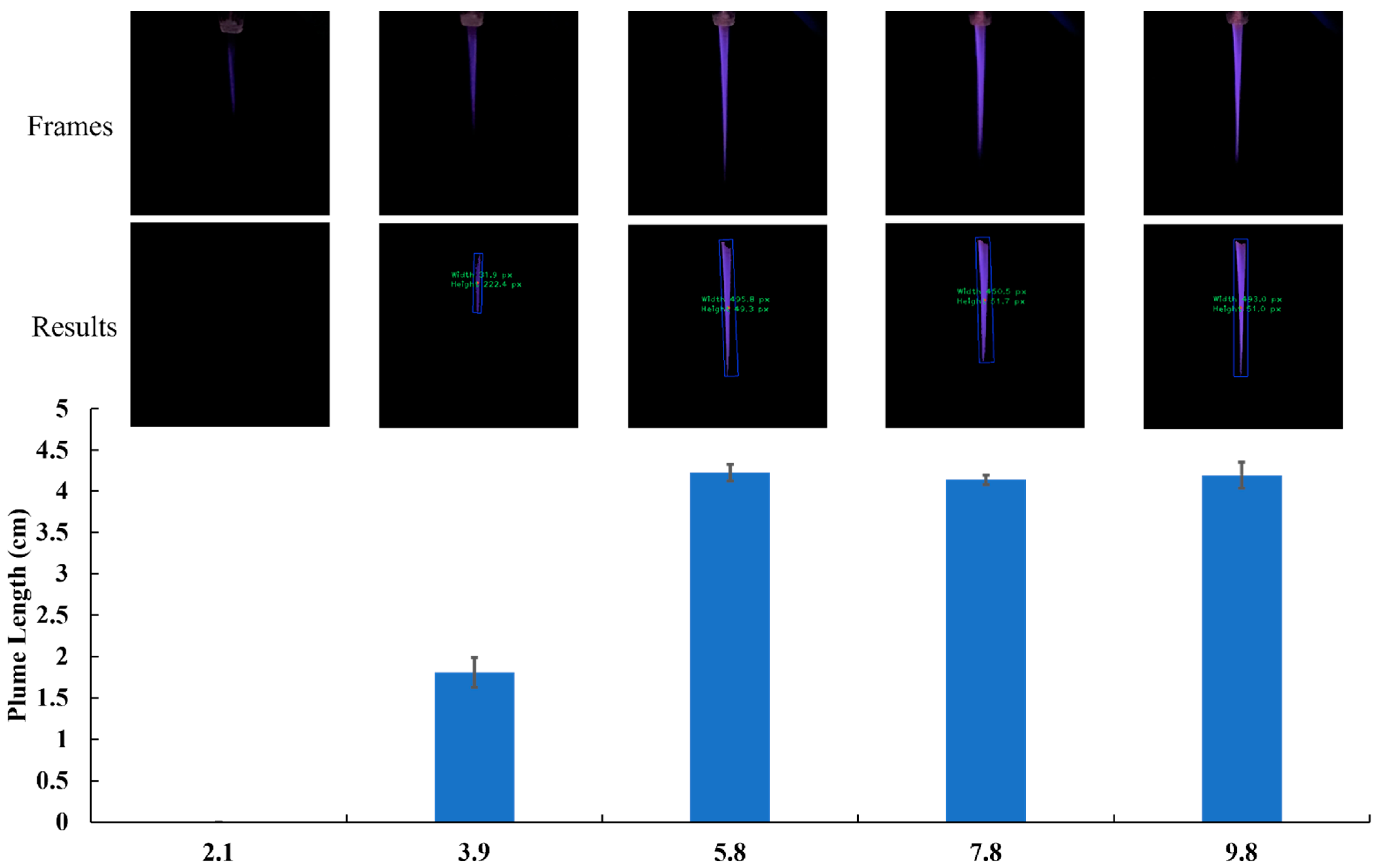
We first studied the potential effect of electrode arrangement on plasma plume length. The results are shown in
Figure 5. Plasma plume lengths remained relatively stable for spacings greater than or equal to 5.8 cm. At an electrode spacing of 4.0 cm, the length of the plasma plume decreased significantly but was still present and detectable by our CV methods. At a gap of 2.1 cm, weak plasma plumes were still formed. However, the weak light intensity was too dim to be recognized by the parameters of our program. The electrode gaps were set to be 9.8 cm in the following tests.
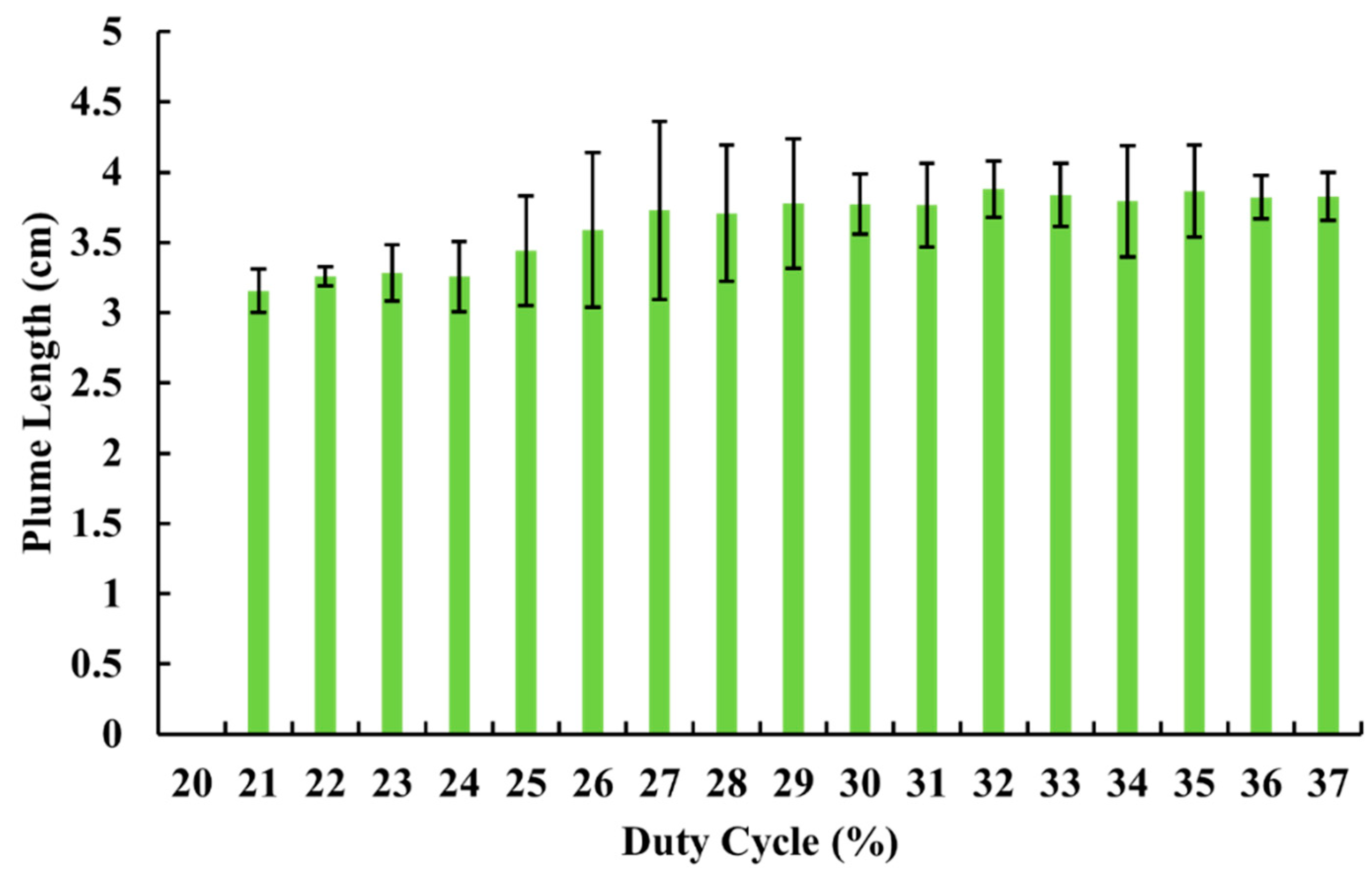
The duty cycle of the input pulse signal does not drastically affect the plasma plume’s length. As shown in
Figure 6, when the duty cycle was less than 20%, no plasma plumes were formed. The further increase in the duty cycle generated a plasma plume longer than 3 cm, which was slightly increased when the duty cycle rose from 21% to 37%. We stopped collection at 37% duty cycle to avoid exceeding the equipment’s current maximums. For duty cycles between 25 and 29%, the standard deviation was relatively large and indicated a higher variability in the plasma output at these parameters. The underlying mechanism is still unknown because there are many intermediate variables between the duty cycle and the plasma plume length. The duty cycle is one of the settings of the pulse signal input.
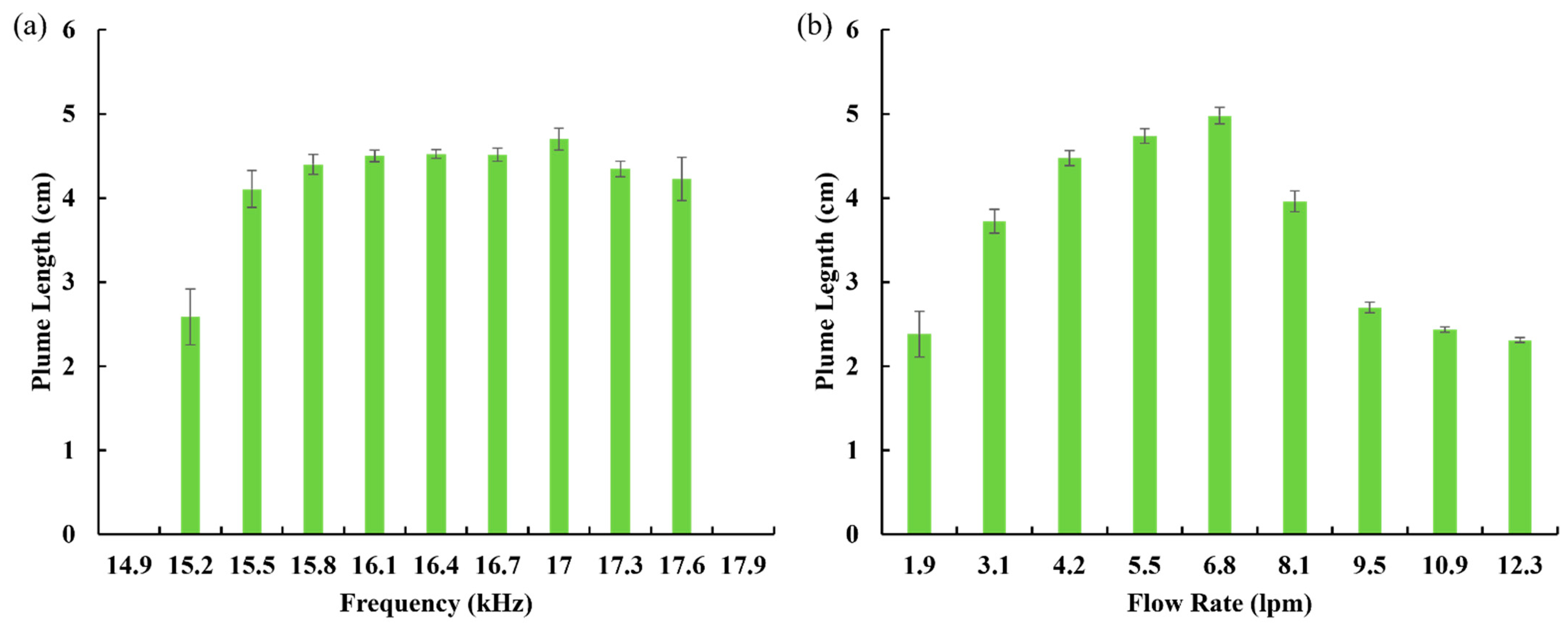
Next, we explored the effect of discharge frequency and helium flow rate on the plasma plume length. As shown in
Figure 7a, discharge frequency was an important operational parameter affecting the cold plasma’s performance. The maximum plasma plume appeared in the middle range of our investigated range (14.9 kHz to 17.9 kHz). Both a too small or too large discharge frequency completely inhibited the plasma plume formation. Moreover, the plasma plume brightness intensity dropped significantly at the ends of the range in addition to the changes in length.
Due to the high monetary cost of compressed inert gases such as helium gas, it is very beneficial to understand how gas flow can be optimized to achieve the best results without wasting gas. In our final demonstration, we used the computer vision approach to explore gas flow effects on the plasma plume’s length. Compared to discharge frequency and duty cycle, helium gas flow has a more gradual impact with respect to the plasma plume’s length. In
Figure 7b there was a clear maximum peak followed by a drop in plasma plume lengths at flows greater than 6.8 lpm. Both plasma plume lengths and standard deviations seemed to reach minimums at higher gas flows. Different from discharge frequency and duty cycle, the flow rate’s effect would not cause a sharp change in the plume length. Together, these three studies demonstrated that the CV approach in this study could quickly recognize and calculate the length of a plasma plume.
4. Discussion
Our preliminary results concur with currently accepted ideas in plasma discharge processes, which again demonstrated the accuracy of computer vision methods in this study. For example, we showed that an electrode gap was an important operational parameter to generate a long plasma plume. Shortening of the plasma output occurred suddenly when the gap reached a critically small value. We also found that, generally, a larger duty cycle was associated with a longer plume. The frequency’s effect, as with the electrode gap’s effect, was not only rapid but could also realize a complete control of the plasma plume’s length, from zero to the maximum value. Finally, we confirmed that the plasma plume’s formation is heavily reliant on the gas flow. Plasma propagation outside the discharge tube is limited primarily by the gas flow, supporting the necessity for an adequately high He–Air ratio. Plasma length can be optimized by a designed control of the discharge frequency and flow rate, as well as the duty cycle. Dissemination and rapid implementation of the computer vision program can easily be achieved, allowing more plasma researchers to investigate the minimums and maximums of the parameters that were hinted at here.
The operational stability of the CAP source is a big concern in plasma medicine [
17]. CAP’s chemical and physical composition is very sensitive to environmental factors such as the purity of the carrying gas and humidity [
18,
19,
20]. To make a stable CAP source, particularly an APPJ source, an intelligent CAP source based on the real-time plasma recognition system and feedback system is necessary [
12,
21,
22]. The morphology of the plasma plume output, particularly the length of an APPJ plume, is an important parameter to estimate its working status. An adequately long plasma plume is challenging in CAP-related research [
10]. Therefore, the fast real-time computer recognition of plasma plumes builds the foundation to realize stable and even self-adaptive CAP sources, which will deeply impact CAP-related studies, particularly in plasma medicine.
5. Conclusions
We have achieved a novel computer vision approach to cold plasma plume recognition and measurement. Our preliminary demonstrations showed that computer vision can be an efficient method for evaluating plasma plume lengths in real time and collecting data points. Furthermore, our studies on the effect of operational parameters on plume length suggest that gas flow, duty cycle, and discharge frequency can be optimized for achieving desired plume lengths. In the future, intelligent CAP devices for use in plasma medicine can combine basic computer vision methods as presented here with more advanced evaluation methods, for example, machine learning, to give adaptive and feedback control capabilities.
Author Contributions
Conceptualization, M.L., D.Y. and M.K.; validation, M.L., D.Y., R.L. and L.L.; writing, M.L., D.Y., R.L. and M.K.; supervision, D.Y. and M.K.; funding acquisition, M.K. All authors have read and agreed to the published version of the manuscript.
Funding
This research was funded by National Science Foundation grant, grant number 1747760.
Institutional Review Board Statement
Not applicable.
Data Availability Statement
Not applicable.
Conflicts of Interest
The authors declare no conflict of interest.
References
- Conrads, H.; Schmidt, M. Plasma Generation and Plasma Sources. Plasma Sources Sci. Technol. 2000, 9, 441–454. [Google Scholar] [CrossRef]
- Kogelschatz, U. Atmospheric-Pressure Plasma Technology. Plasma Phys. Control. Fusion 2004, 46, B63. [Google Scholar] [CrossRef]
- Fridman, G.; Friedman, G.; Gutsol, A.; Shekhter, A.B.; Vasilets, V.N.; Fridman, A. Applied Plasma Medicine. Plasma Processes Polym. 2008, 5, 503–533. [Google Scholar] [CrossRef]
- Graves, D.B. Mechanisms of Plasma Medicine: Coupling Plasma Physics, Biochemistry, and Biology. IEEE Trans. Radiat. Plasma Med. Sci. 2017, 1, 281–292. [Google Scholar] [CrossRef]
- Weltmann, K.D.; Kindel, E.; von Woedtke, T.; Hähnel, M.; Stieber, M.; Brandenburg, R. Atmospheric-Pressure Plasma Sources: Prospective Tools for Plasma Medicine. Pure Appl. Chem. 2010, 82, 1123–1237. [Google Scholar] [CrossRef]
- Kogelschatz, U. Dielectric-Barrier Discharges: Their History, Discharge Physics, and Industrial Applications. Plasma Chem. Plasma Process 2003, 23, 1–46. [Google Scholar] [CrossRef]
- Lu, X.; Naidis, G.V.; Laroussi, M.; Ostrikov, K. Guided Ionization Waves: Theory and Experiments. Phys. Rep. 2014, 540, 123–166. [Google Scholar] [CrossRef]
- Keidar, M. Plasma for Cancer Treatment. Plasma Sources Sci. Technol. 2015, 24, 033001. [Google Scholar] [CrossRef]
- Schutze, A.; Jeong, J.Y.; Babayan, S.E.; Park, J.; Selwyn, G.S.; Hicks, R.F. The Atmospheric-Pressure Plasma Jet: A Review and Comparison to Other Plasma Sources. IEEE Trans. Plasma Sci. 1998, 26, 1685–1694. [Google Scholar] [CrossRef]
- Lu, X.; Jiang, Z.; Xiong, Q.; Tang, Z.; Hu, X.; Pan, Y. An 11 Cm Long Atmospheric Pressure Cold Plasma Plume for Applications of Plasma Medicine. Appl. Phys. Lett. 2008, 92, 2006–2008. [Google Scholar]
- Sousa, J.S.; Niemi, K.; Cox, L.J.; Algwari, Q.T.; Gans, T.; O’Connell, D. Cold Atmospheric Pressure Plasma Jets as Sources of Singlet Delta Oxygen for Biomedical Applications. J. Appl. Phys. 2011, 109, 123302. [Google Scholar] [CrossRef] [Green Version]
- Lin, L.; Keidar, M. A Map of Control for Cold Atmospheric Plasma Jets: From Physical Mechanisms to Optimizations. Appl. Phys. Rev. 2021, 8, 011306. [Google Scholar] [CrossRef]
- Lyu, Y.; Lin, L.; Gjika, E.; Lee, T.; Keidar, M. Mathematical Modeling and Control for Cancer Treatment with Cold Atmospheric Plasma Jet. J. Phys. D Appl. Phys. 2019, 52, 185202. [Google Scholar] [CrossRef]
- Lin, L.; Yan, D.; Lee, T.; Keidar, M. Self-Adaptive Plasma Chemistry and Intelligent Plasma Medicine. Adv. Intell. Syst. 2022, 4, 2100112. [Google Scholar] [CrossRef]
- Keidar, M.; Yan, D.; Beilis, I.I.; Trink, B.; Sherman, J.H. Plasmas for Treating Cancer: Opportunities for Adaptive and Self-Adaptive Approaches. Trends Biotechnol. 2018, 36, 586–593. [Google Scholar] [CrossRef]
- Lin, L.; Hou, Z.; Yao, X.; Liu, Y.; Sirigiri, J.R.; Lee, T.; Keidar, M. Introducing Adaptive Cold Atmospheric Plasma: The Perspective of Adaptive Cold Plasma Cancer Treatments Based on Real-Time Electrochemical Impedance Spectroscopy. Phys. Plasmas 2020, 27, 063501. [Google Scholar] [CrossRef]
- Yue, Y.; Wu, F.; Cheng, H.; Xian, Y.; Liu, D.; Lu, X.; Pei, X. A Donut-Shape Distribution of OH Radicals in Atmospheric Pressure Plasma Jets. J. Appl. Phys. 2017, 121, 33302. [Google Scholar] [CrossRef]
- Lin, L.; Lyu, Y.; Trink, B.; Canady, J.; Keidar, M. Cold Atmospheric Helium Plasma Jet in Humid Air Environment. J. Appl. Phys. 2019, 125, 153301. [Google Scholar] [CrossRef]
- Dobrynin, D.; Friedman, G.; Fridman, A.; Starikovskiy, A. Inactivation of Bacteria Using Dc Corona Discharge: Role of Ions and Humidity. New J. Phys. 2011, 13, 103033. [Google Scholar] [CrossRef]
- Shimizu, K.; Umeda, A.; Blajan, M. Surface Treatment of Polymer Film by Atmospheric Pulsed Microplasma: Study on Gas Humidity Effect for Improving the Hydrophilic Property. Jpn. J. Appl. Phys. 2011, 50, 08KA03. [Google Scholar] [CrossRef]
- Bonzanini, A.D.; Shao, K.; Stancampiano, A.; Graves, D.B.; Mesbah, A. Perspectives on Machine Learning-Assisted Plasma Medicine: Toward Automated Plasma Treatment. IEEE Trans. Radiat. Plasma Med. Sci. 2022, 6, 16–32. [Google Scholar] [CrossRef]
- Mesbah, A.; Graves, D.B. Machine Learning for Modeling, Diagnostics, and Control of Non-Equilibrium Plasmas. J. Phys. D Appl. Phys. 2019, 52, 30LT02. [Google Scholar] [CrossRef] [Green Version]
Figure 1.
Schematic illustration of double–ring electrodes’ APPJ source. IGBT: insulated–gate bipolar transistor (IGBT). Oscillating high voltage was generated between two copper electrodes. Throughout this whole study, “plasma plume” just means the violet plasma formed below the nozzle, it does not mean the white lighting area between two electrodes.
Figure 2.
Real–time computer recognition system. (a) Full schematic of plasma plume and image analysis setup shows how plasma was generated, how measurements were taken, and component connections. The specific camera used was an iPhone 11 attached via cable to a laptop computer running the software where video stream from the camera was accessed. The electrode gap can be easily varied by choosing any two electrodes of the five copper ring settings. (b) ArUco marker used in camera calibration. ArUco markers are frequently used in computer vision applications because there is significant open-source material supporting them. This project takes advantage of the library function cv2.aruco.detectMarkers() to return pixel (px) coordinates of ArUco markers from a specific set.
Figure 3.
Program flow chart. Here, we show the main program and data collection routine. Once the .py file was run from the command line, a whole loop isolates frames, identifies plasma, and measures it.
Figure 3.
Program flow chart. Here, we show the main program and data collection routine. Once the .py file was run from the command line, a whole loop isolates frames, identifies plasma, and measures it.
Figure 4.
The main GUI windows of the program. (a) The frame window was inputted; (b) a mask was created to identify purple; (c) and a bounding box was drawn to surround the plasma plume region. Box dimensions on the screen were displayed in pixels so the program could start without relying on camera calibration. Only if data were collected was calibration required. In this case, pixel values were converted to centimeters and saved if the camera position was calibrated using an ArUco marker.
Figure 5.
Electrodes’ gap affects plasma plume’s length. Electrodes’ gap was varied from 2.1 cm to 9.8 cm, while discharge frequency, duty cycle, and gas flow were held constant at 16 kHz, 25%, and 4.2 lpm, respectively. These photos are images of the live video stream fed into the program (top row: frames) and the output after selecting only the plasma regions (bottom row: results). All experiments were repeated three times. The results were shown as the mean ± standard deviation (error bar).
Figure 6.
Duty cycle’s effect on plume length. The duty cycle varied between 20 and 37%, while all other parameters were held constant. Gas flow was 4.2 lpm, and frequency was 16 kHz. Electrode spacing was 9.8 cm. All experiments were repeated three times. The results are shown as the mean ± standard deviation (error bar).
Figure 7.
Discharge frequency and helium flow rate strongly affect plasma plume length. (a) Discharge frequency effect. Duty cycle and gas flow were held at 25% and 4.2 lpm, respectively. (b) Gas flow effect. The duty cycle and discharge frequency were held at 25% and 16 kHz, respectively. All experiments were repeated three times. The results are shown as the mean ± standard deviation (error bar).
Table 1.
Upper and lower HSV values used for plume identification by color were identified from a typical plasma plume image.
Table 1.
Upper and lower HSV values used for plume identification by color were identified from a typical plasma plume image.
| | Lower | Upper |
|---|
| Hue | 120 | 180 |
| Saturation | 119 | 255 |
| Value | 115 | 255 |
| Publisher’s Note: MDPI stays neutral with regard to jurisdictional claims in published maps and institutional affiliations. |
© 2022 by the authors. Licensee MDPI, Basel, Switzerland. This article is an open access article distributed under the terms and conditions of the Creative Commons Attribution (CC BY) license (https://creativecommons.org/licenses/by/4.0/).


