Abstract
This article considers the numerical solution of the direct and inverse problems of the gas lift process in oil production, described by a system of hyperbolic equations. The inverse problem is reduced to an optimal control problem, where the control is the initial velocity of the gas. To minimize the quadratic objective functional, the gradient method is used, in which the gradient is determined using the conjugate equation method. The latter involves constructing a conjugate problem based on the Lagrange identity and the duality principle. Solving the conjugate problem allows us to obtain an analytical expression for the gradient of the functional and effectively implements the Landweber iterative method. A numerical experiment was carried out that confirmed the effectiveness of the proposed method in optimizing the parameters of the gas lift process.
1. Introduction
The gas lift process is one of the most widely used methods of mechanized oil production, in which compressed gas is pumped into the annular space of a well to reduce the density of the gas–liquid mixture (GLM), reduce hydrostatic pressure, and, as a result, facilitate the lifting of production to the surface. The gas lift system includes two key areas: the annular space between the casing and the tubing through which the gas moves and the lift, an internal well through which a mixture of oil, gas, and water is lifted to the surface.
The dynamics of gas and gas–liquid mixture movement in a well can be described by a system of hyperbolic partial differential equations, in which pressure and volumetric gas flow rate are the main variables. These models take into account the spatio-temporal distribution of parameters and allow for the analysis of processes under different boundary and initial conditions [1].
One of the urgent tasks in the context of gas lift process management is the determination of the optimal initial conditions (for example, gas velocity distribution) that ensure the required oil production with a minimum volume of injected gas. This problem is framed as an optimal control problem, where the functionality reflecting the well production indicators is optimized. The use of numerical optimization methods based on models obtained from simulators such as PIPESIM is found, for example, in [2], and the problems related to distributing gas injection between wells are solved using mathematical programming methods and evolutionary algorithms [3].
Modern methods for solving inverse problems arising in mathematical physics involve reducing them to optimal control problems with partial differential equations as constraints. The classical theory of such problems was developed by J.L. Lions [4,5], and the method of conjugate equations, based on the Lagrange identity and the duality principle, was studied in detail in the works of Agashkov [6], Marchuk [7] and other authors. The conjugate problem method allows us to effectively calculate the gradient of the objective functional, which makes it possible to apply gradient optimization methods [8,9].
Additional interest in the application of the conjugate equation method is due to its successful use in various fields—from string vibration control [8] to numerical solutions of acoustic problems and problems involving regularization methods [10,11,12,13,14,15,16]. An example of this work is study [17], which deals with the modeling and optimization of an industrial rotary kiln (RHF) used for processing solid metallurgical waste. In the study, a numerical model is built based on heat transfer and gas dynamics equations, and then a surrogate model is built using machine learning methods. Optimization is performed using industrial data to minimize energy costs. This methodology, which combines direct modeling and numerical optimization methods integrated with real data, is of great interest and can be adapted for gas lift process problems, where it is also necessary to determine the optimal initial pressure distribution or gas flow rate.
A number of papers have proposed effective numerical methods for solving applied problems in mathematical physics. In [18], an algorithm was developed for solving the inverse problem for the acoustics equation using the gradient method, which ensures high accuracy of reconstruction of unknown parameters. In [19], an approach to numerical modeling of the transport of pollutants in the atmosphere is presented, which makes it possible to increase the accuracy of the forecast in an industrial environment. Both works demonstrate the importance of using modern computational methods to solve inverse and predictive problems in various fields.
Despite the simplicity of the mathematical model used, the novelty of this work lies in the formalization and numerical solution of the inverse problem of determining the initial gas velocity function, , for a given flow rate distribution, , at time . Such a formulation is rarely considered in relation to gas lift processes. In this work, a numerical algorithm is developed based on the method of conjugate equations, the duality principle, and the Landweber method, which allows for the effective solution of such problems while taking into account the design features of the well (two zones with different characteristics and transition conditions at the point ).
The aim of this work is to reconstruct the initial distribution of gas velocity in a system described by hyperbolic equations using additional information about the state of the system at the final moment in time. This task arises when it is necessary to clarify the initial conditions for modeling the gas lift process, particularly when direct measurements at the depth of the well are difficult or impossible.
Unlike existing methods, this paper uses the conjugate equation method, which allows us to effectively find the gradient of the target functional and implement an iterative optimization procedure. This approach ensures high accuracy in solving the inverse problem with minimal computational costs. The obtained results confirm the applicability of the developed numerical method for restoring hidden parameters and optimizing the operating conditions of gas lift wells.
2. Materials and Methods
2.1. Statement of Direct and Inverse Problems
The mathematical model of the gas lift well operation is described using the following linear system of differential equations [1]:
where is time; is a coordinate along the well depth; is the pressure; is the volume flow rate of gas; is the cross-sectional area of the well; c is the speed of sound in liquid; l is the well depth; and a is a coefficient that depends on the input parameters.
Parameters and characterize the combined effect of gravitational acceleration and hydraulic resistance on gas movement in the annular space and lift, respectively. These coefficients reflect energy losses due to friction and lifting along the well.
Variables and denote the speed of sound in a gas–liquid medium in different zones of the well: —in the annular space, where gas predominantly moves, and —inside the lifting pipe, where a mixture of gas and oil moves. The difference between and is due to differences in the composition and density of the media, which is critical for the correct modeling of wave processes.
The initial conditions are as follows:
and the boundary conditions are as follows:
where is the volumetric flow rate from the reservoir; is the reservoir pressure; is the initial gas pressure; is the initial gas volume; is the discharge pressure; and is the discharge volume.
We will reduce the system of hyperbolic Equations (1) and (2) to one second-order equation. To accomplish this, we must find the derivative with respect to x from Equation (1).
Using Equation (2), we can determine the derivative with respect to .
Let us substitute (7) into Equation (8). Then, Equation (8) assumes the following form:
The initial conditions are as follows:
and the boundary conditions are as follows:
where is the initial rate of gas displacement.
In the direct problem, it is necessary to find based on the given functions , , , and .
The inverse problem is formulated as follows:
The main issue with the inverse problem deriving from Equations (9)–(12) with additional conditions (13).
The transformation of the system of hyperbolic equations into one second-order equation allows us to move from the description of the interacting quantities, and , to focusing on one objective function—the volumetric gas flow rate, . This significantly simplifies both the numerical implementation of the direct problem and the formulation of the inverse problem, in which the behavior of the function, , at the final moment of time is used as the observed data.
In addition, the use of one second-order equation allows us to explicitly formulate the conjugate problem and calculate the gradient of the target functional, which forms the basis of the conjugate equation method.
2.2. Statement of the Variational Problem
One of the most widely used methods for solving inverse problems of mathematical physics is reducing Equations (9)–(12) and (13) to an optimal control problem.
The aim of the problem is to find the initial values of so that the corresponding solution to Equation (9) approaches the specified desired value of .
More precisely, our problem is to minimize the objective functional, as follows:
on the admissible control set, .
Here, represents the solution’s, , dependence on Equations (9)–(12) and (13) using the initial conditions.
Minimize the functional using the gradient method as follows [20]:
where is a relaxation parameter.
The choice of relaxation parameter determines the gradient method, which plays an important role. The relaxation parameter α determines the length of the gradient descent step and has a direct impact on the convergence rate of the iteration process. A value of α that is too large can lead to divergence of the method, while a value that is too small can lead to slow convergence.
In practice, the choice of is made either empirically (based on preliminary tests) or using adaptive strategies such as the steepest descent method, where is selected at each iteration to minimize the functional along the current direction. In this study, α was taken as constant and selected in such a way as to ensure a stable monotonic decrease in the values of the functional with an acceptable number of iterations.
The procedure for obtaining the variational and conjugate problems is as follows:
- Let us consider the variation of the functional, , under the perturbation, .
- We introduce the perturbed solution, , and define
- We perform a convolution of the variation through the unknown function, satisfying the following conjugate equation:
- 4.
- Then, the Frechet derivative of the functional takes the following the form:
All intermediate calculations, including integration by parts and proof of the identity, are given in Appendix A.
2.3. Landweber Algorithm (Simple Iteration Method)
- We set the initial approximation, .
- Suppose that is already known; then, we solve the direct problem (9)–(12).
- Calculate the value of the following functional:
- If the current value of the functional, , is not small enough, solve the conjugate problem (16)–(18).
- Calculate the gradient of the following functional:
- Calculate the following approximation:
2.4. Numerical Solutions for the Direct and Conjugate Problem
Here, we present a method for numerically solving both direct and conjugate problems using the finite difference method [21]. To achieve this, the solution area is divided into a uniform grid, and the initial differential equations are approximated by difference schemes. The first part describes the process of solving a direct problem, including building a grid, approximating equations, and implementing boundary conditions. In the second part, the solution of the conjugate problem is considered in detail. A similar difference technique considers the specifics of the boundary and initial conditions. The numerical schemes obtained make it possible to efficiently solve both problems in a discrete formulation.
2.4.1. Scheme for Solving a Direct Problem
Let us approximate the direct problem in (9)–(12). Let be the number of nodes in the uniform grid on the interval and let be the number of nodes in the uniform grid on the interval .
Construct a grid, , with a step of , , where and are positive integers in the domain of = ().
Then, in the grid, , we can write the following difference direct problem. Thus, problems (9)–(12) assume the following form:
From Equations (19)–(22) we obtain the following equations:
Solving the problem, we obtain a trace of the solution as follows:
2.4.2. A Scheme for Solving the Conjugate Problem
For the conjugate problem, we use the same grid as that of the direct problem. Thus, the problem in (16)–(18) takes the following form:
From Equations (27)–(29) we derive the following equations:
2.5. Study of the Approximation and Stability of a Family of Difference Schemes
The mathematical model of the gas lift well operation is described using the following linear system of differential equations:
The implicit difference scheme for Equations (1) and (2) is as follows:
that is
Here, and are the values of the functions and at the point on the time layer , with the following initial conditions:
and boundary conditions, respectively
Let us rewrite (36)–(37) in the following form:
where
It can be seen that the count can be started from the point . Then, we obtain the following equations:
by multiplying Equation (45) by and summing it with the first one, we obtain the following equation:
Using this formula, we derive as follows:
Substituting in (45), we obtain .
With and , it is possible to calculate all values of and up to some and taking ; find and for , etc.
In the general case, to determine we obtain the following formula:
Let us consider the following family of schemes defined on a four-point template:
with the following initial conditions:
and the following boundary conditions:
Schemes (36) and (37) belong to this family and correspond to .
Let us calculate the residual for this system of difference equations.
Let us use the Taylor series expansion as follows:
Substituting these expansions into , we obtain the following equation:
Similarly, we obtain the following equation:
Let us expand functions and with respect to the variable as follows:
Find the backward difference derivative as follows:
Similarly, we obtain the following equation:
By substituting (37)–(40) into (55) and (56), we obtain the following equations:
To make further calculations for residuals and more convenient, we assume the following equalities:
Let us expand the terms in a Taylor series with respect to in the vicinity of the point .
Then, from (61)–(62), taking assumption (63) into account, we obtain the following equations:
From the main, Equations (34) and (35), we derive the following equations:
Substituting these expressions into (69), we obtain the following expressions:
It is clear that the terms containing cancel each other out and we obtain the following equations:
Let us expand the second derivatives in a Taylor series with respect to t in the vicinity of the point .
Suppose that .
Taking into account (72) from (70) and (71), we obtain the following equations:
From the system of Equations (34) and (35), we obtain the following equation:
Consider the following equations:
As well as the following equations:
We obtain the following equations:
It can be seen that the scheme with weights has a second-order approximation.
if the following equality holds:
and —the first order, .
Stability is based on the initial data.
Let us now show that the scheme of the family of schemes with weights (48)–(54) is stable with respect to the initial data when the following condition is met:
Using the method of energy inequalities, we obtain the following equation:
We can consider the sum as follows:
We will introduce the grid, , in the segment .
The scalar product and norm are defined as follows:
taking the following equations into account:
and assuming that .
We can rewrite the scheme (75) in the following form:
Multiply this equation by as follows:
We transform the first term as follows:
Then, we obtain the following equation:
If we combine the second and third terms, we obtain the following equation:
Multiplying by and summing up over all grid nodes, we obtain the following equation:
We write out the difference derivative with respect to x in the first term and then obtain the following equation:
We expand the sum, cancel the terms, and derive the following equation:
Here, because .
Finally, we obtain the following identity:
From identity (77), it can be seen that if the following condition is met:
i.e., then we obtain the following equation:
Scheme (75) is stable in the following energy norm:
3. Results and Discussion
Numerical Solution for the Problem
Computational Experiment
The initial data for the computational experiment are as follows: is the volumetric flow rate of injected gas (); is the initial pressure distribution (); is the well depth (m); is the hydraulic resistance in the ring; is the hydraulic resistance in the pipe; is the effective diameter of the well annular space (m); and is the internal diameter of the well (m).
is the gas density (); is the oil density (); g = 9.8 is the gravity acceleration (); is the speed of sound in the annular space (m/s); is the speed of sound in the pipe (m/s); is the radius of the annular space (m); is the radius of the inner pipe (m); is the cross-sectional area of the pipe of the well’s annular space (); is the cross-sectional area of the inner pipe of the well (); is averaged over the cross-section speed of the mixture in the ring (m/s); and is the average cross-sectional speed of the mixture in the pipe (m/s).
The coefficients in the ring and pipe are described as follows:
Calculations of the test problem were performed for the parameters , , , , and . The step of gradient descent is , the exact solution of which is known, as follows:
The initial approximation is as follows:
Figure 1 shows a graph of change in the functional during the numerical solution process of the inverse problem. The graph demonstrates a monotonic decrease in functional values during the iteration process.
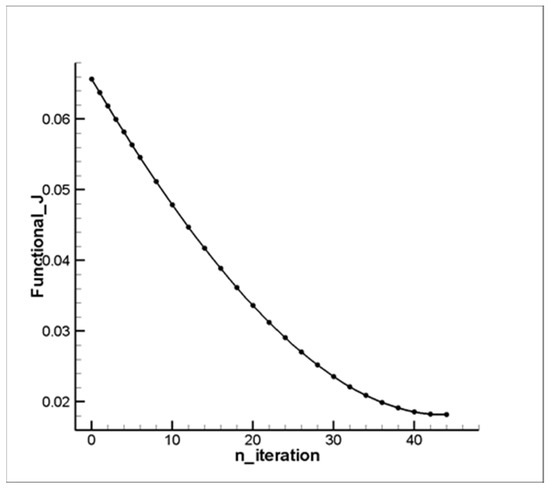
Figure 1.
Graph of decreasing functional .
To quantitatively assess the accuracy of the numerical method, an error analysis was performed between the approximate and exact solution of the function . The Euclidean (discrete ) error norm was used as a measure as follows:
When using the gradient descent step, , and 46 iterations, the error value was . This confirms the good accuracy of the approximation, especially in the central part of the region, while the main discrepancies are concentrated in the interval , where high gradients of the function are observed.
The convergence analysis of the functional showed its monotonous decrease from the initial value to the level of over 46 iterations. Further increases in the number of iterations did not provide significant improvement, which indicates the achievement of the optimum and the stability of the method. Thus, the proposed numerical method provides a reliable approximation of the desired function and demonstrates stable behavior with respect to computational costs.
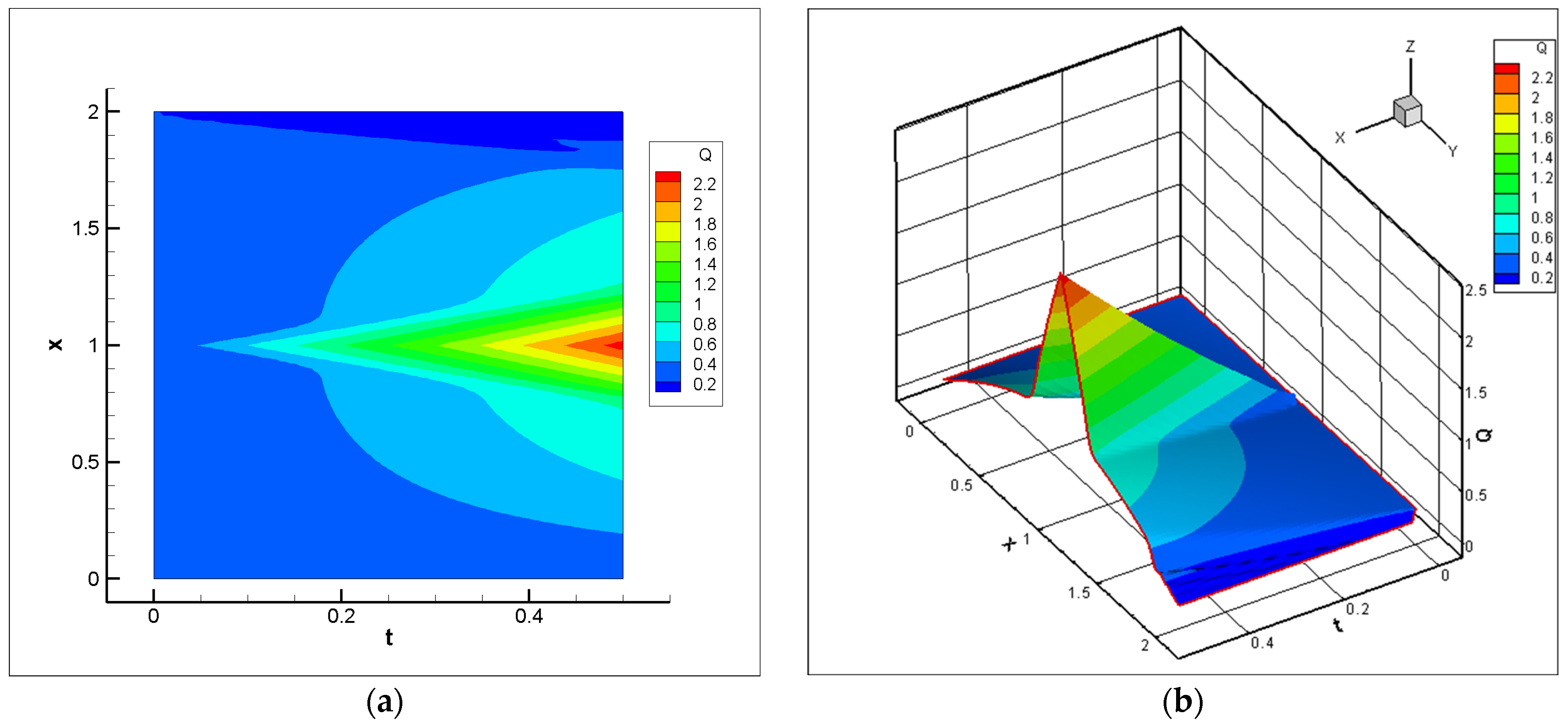
Figure 2 shows (a) a two-dimensional and (b) a three-dimensional picture of the smooth distribution of the function , reflecting correct wave and symmetry development. The range of changes in the function is wider, and the changes in gradient are smoother.

Figure 2.
An exact solution, , using the true initial condition, (a) shows the smooth wave propagation and symmetric distribution of the function across the domain. (b) illustrates the behavior of near regions where high gradients appear, highlighting the accuracy of the true initial condition.
Figure 3 shows (a) two-dimensional and (b) three-dimensional solutions, which diverge for an approximate value of the initial condition, , in areas close to and . A distortion in the shape and a narrowing in the range of maximum values of the function indicate incomplete convergence of the iterative process.
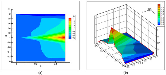
Figure 3.
An approximate solution, using the initial condition, , reconstructed using the Landweber method. (a) shows the distribution of the approximate solution of , showing deviations in waveform and amplitude. (b) identifies regions near and where the approximation diverges from the exact solution.
The main discrepancies between the exact and approximate solutions are in the region of , where the values of on the right graph are smaller than the exact solution. This discrepancy is caused by insufficient correction of the initial condition in the Landweber method at this stage. The exact solution reflects the correct distribution of wave processes, while the approximate solution shows minor deviations in areas with high gradients. Additional iterations of the Landweber method can improve convergence and reduce discrepancies between the numerical and exact solutions. The graphs clearly show the importance of accurately approximating the initial condition, , to achieve high accuracy in modeling gas lift wells.
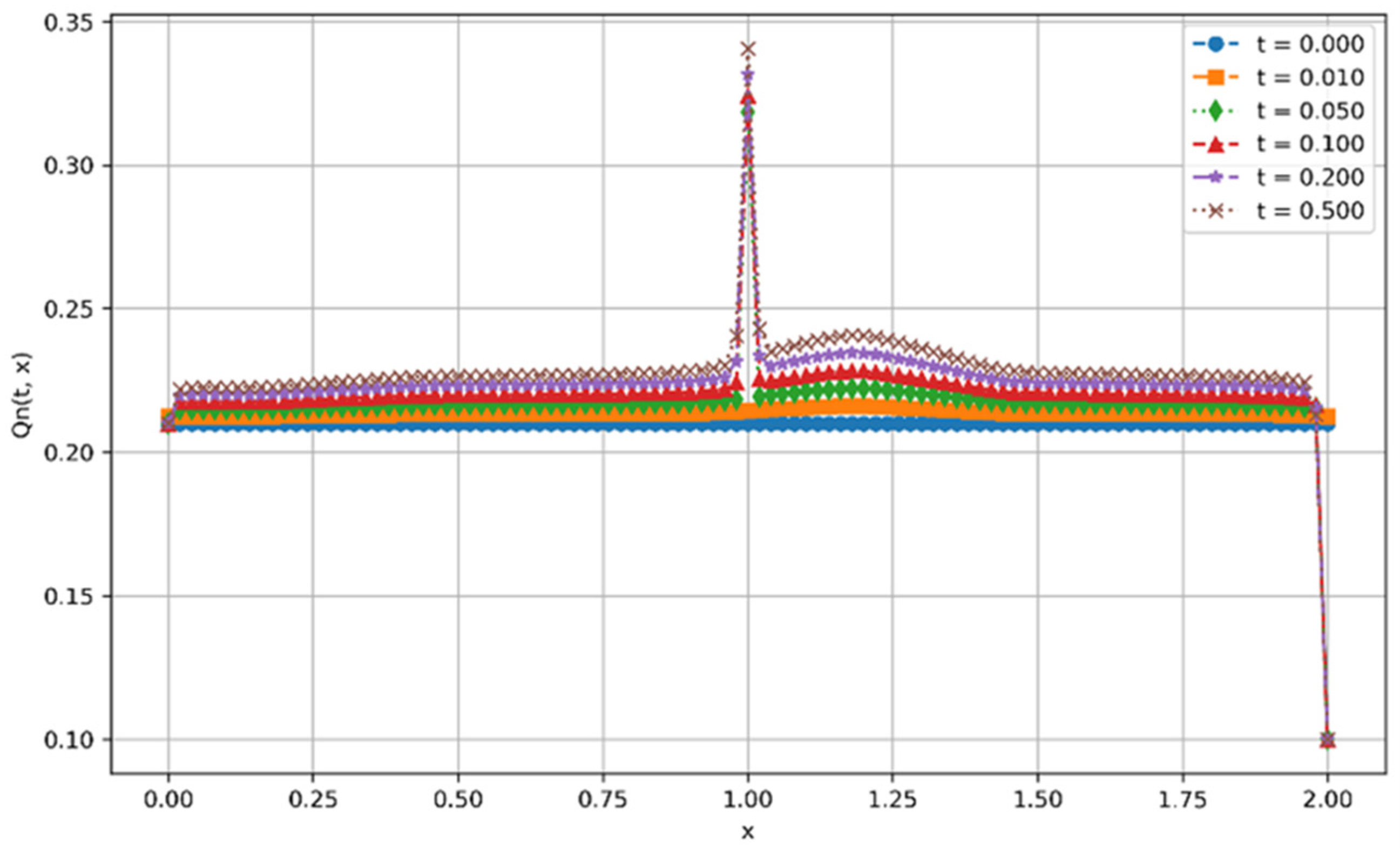
Both graphs (Figure 4 and Figure 5) show a smooth change in the function along the x-axis for small values of time intervals, t. As the time increases, an increase in the amplitude is observed in the central part of the graph, near . This increase indicates the formation of a localized maximum, which is typical for solutions of the considered system of equations. The function demonstrates a more pronounced symmetry with respect to the center than the function , indicating the high accuracy of the exact solution.
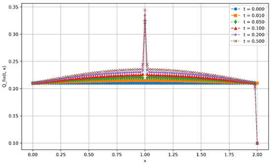
Figure 4.
Graph of the function for different values of with precisely specified initial conditions.
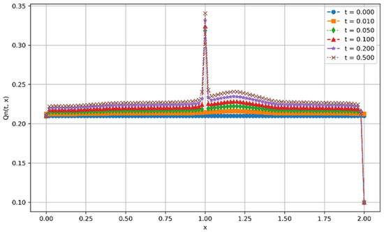
Figure 5.
Graph of the function for different values of with approximate initial conditions.
In both cases, a distinct peak is visible in the vicinity of With increasing time, this peak becomes stronger and reaches its maximum values at . However, in the right graph, which represents an approximate solution, the central peak shows a slight shift and fluctuation, which may indicate the approximation’s inaccuracy.
At the initial time intervals, the values of the function at the boundaries and remain practically unchanged. However, with an increase in the time parameter, t, a decrease in the values of the function at the boundaries is observed. This phenomenon is consistent with the physical interpretation of the boundary conditions and reflects the expected behavior of the solution for the system.
The proposed method has important practical applications, as it helps optimize the parameters of the gas lift process and minimizes gas consumption for maximum oil production. This optimization leads to a significant reduction in operating costs during oil production, which is especially important for aging fields with low flow rates.
4. Conclusions
In this paper, a numerical method for solving the direct and inverse problems of the gas lift process in oil production, based on the method of conjugate equations, is developed and implemented. The key novelty of the method lies in the application of a variational formulation and the construction of a conjugate problem for calculating the gradient of the functional, which allows us to effectively solve the inverse problem of restoring the initial distribution of gas velocity for a given final state.
Unlike traditional empirical or heuristic methods for optimizing gas lift processes, the proposed method is based on a rigorous mathematical framework and ensures controlled convergence. This allows us not only to increase the accuracy of calculations but also to reduce the volume of injected gas while maintaining the level of oil production, which is of great practical importance.
The conducted numerical experiments confirmed the effectiveness of the method: high accuracy in approximating the target function was achieved in a limited number of iterations, while stable and reproducible results were obtained. The method can be used to optimize the operating parameters of gas lift wells and can also be adapted to more complex models, including multidimensional and nonlinear settings.
The practical significance of the proposed method lies in its potential integration into software packages for managing oil production at gas lift wells. By restoring the optimal initial distribution of gas velocity, a more precise adjustment of the injection mode is ensured, which allows for the following benefits:
- -
- Reduce the volume of gas consumed while maintaining the production level.
- -
- Adapt control to changing reservoir and well characteristics.
- -
- Increase operating efficiency without the need to install additional sensors.
- -
- Predict and minimize the risks of underloading or the over-consumption of gas.
Thus, this study represents a significant contribution to the development of optimal control methods for problems described by hyperbolic equations and opens up opportunities for further applied developments in modeling oil and gas processes. The method can also serve as a decision support tool in intelligent oil field management systems, especially when implementing automation and digitalization in oil production.
Author Contributions
Conceptualization, S.E.K. and N.M.T.; methodology, A.K.T. and N.M.T.; software, A.K.T. and S.E.K.; validation, S.E.K. and A.K.T.; formal analysis, S.E.K. and A.K.T.; investigation, A.K.T.; resources, S.E.K. and A.K.T.; data curation, S.E.K. and A.K.T.; writing—original draft preparation, A.K.T.; writing—review and editing, A.K.T.; visualization, A.K.T.; supervision, N.M.T.; project administration, A.K.T. and N.M.T.; funding acquisition, A.K.T. All authors have read and agreed to the published version of the manuscript.
Funding
This research was funded by the Science Committee of the Ministry of Science and Higher Education of the Republic of Kazakhstan (Grant No. AP22683374—“Numerical solution of the multiphase dynamic model of the gas-lift process”).
Data Availability Statement
The original contributions presented in this study are included in the article. Further inquiries can be directed to the corresponding authors.
Conflicts of Interest
The authors declare no conflicts of interest.
Appendix A
Calculate the first variation of the integral functional (14).
as
On the other hand, using the definition of the Frechet derivative, we obtain the following equation:
Let us introduce the notations as follows:
Now, we can consider the perturbed problem corresponding to Equations (9)–(12).
We can subtract Equations (A2)–(A5) from Equations (9)–(12) and obtain the following expressions for :
Let us consider an expression identically equal to zero obtained from (A6) by multiplying it by a still unknown function, , and integrating with respect to and .
Here,
Integrating this expression by parts, we obtain the following expressions:
A repeated integration by parts results in the following expressions:
Taking into account the boundary conditions in (22)–(24), we obtain the following equations:
From the first term on the right-hand side of (A10), we obtain the conjugate control. From the requirement that is equal to zero on the boundary of the domain, we construct the following retrospective problem at
The remaining terms of expression (A10) lead to the following lemma:
Lemma A1.
Let be given elements.
If is a solution to the problem in (9)–(12), and is a solution to the conjugate problem in (A11)–(A13), then the following identity must hold:
Condition (A14), considering the boundary conditions (A7) and (A13) and the definition of the Frechet derivative (A1), will be written as follows:
This condition follows from the Lagrange principle.
It is called the principle of duality.
References
- Aliyev, F.A.; Mutalimov, M.M. Algorithm for solving the trajectory construction and control problem in gas-lift oil production. In Report of the National Academy of Sciences of Azerbaijan; National Academy of Sciences of Azerbaijan: Baku, Azerbaijan, 2009. [Google Scholar]
- Mehregan, M.R.; Mohaghar, A.; Esmaeili, A. Developing a mathematical model for optimizing oil production using gas-lift technology. Int. J. Eng. Res. Appl. 2016, 9, 24–32. [Google Scholar]
- Jung, S.-Y.; Lim, J.-S. Optimization of gas lift allocation for improved oil production under facilities constraints. Geosyst. Eng. 2016, 19, 39–47. [Google Scholar] [CrossRef]
- Lions, J.L. Optimal Control of Systems Governed by Partial Differential Equations; Springer: Berlin/Heidelberg, Germany, 1971. [Google Scholar]
- Lions, J.L.; Magenes, E. Non-Homogeneous Boundary Value Problems and Applications; Springer: Berlin/Heidelberg, Germany, 1972; Volume II. [Google Scholar]
- Agoshkov, V.I. Optimal Control Methods and the Method of Conjugate Equations in Problems of Mathematical Physics; Institute of Higher Mathematics RAS: Moscow, Russia, 2003; 256p. [Google Scholar]
- Marchuk, G.I. Conjugate Equations and Their Applications. Proc. IMM URO RAS 2006, 12, 184–195. [Google Scholar]
- Il’in, V.A.; Moiseev, E.I. Optimization of boundary controls by displacements at two ends of a string during an arbitrary sufficiently large time interval. Dokl. Math. 2007, 76, 828–834. [Google Scholar]
- Temirbekov, A.N.; Temirbekova, L.N.; Zhumagulov, B.T. Fictitious domain method with the idea of conjugate optimization for non-linear Navier-Stokes equations. Appl. Comput. Math. 2023, 22, 172–188. [Google Scholar] [CrossRef]
- Kasenov, S.E.; Tleulesova, A.M.; Sarsenbayeva, A.E.; Temirbekov, A.N. Numerical Solution of the Cauchy Problem for the Helmholtz Equation Using Nesterov’s Accelerated Method. Mathematics 2024, 12, 2618. [Google Scholar] [CrossRef]
- Arguchintsev, A.V.; Poplevko, V.P. An optimal control problem by hyperbolic system with boundary delay. Bulletin of Irkutsk State University. Mathematics 2021, 35, 3–17. [Google Scholar] [CrossRef]
- Arguchintsev, A.V.; Krutikova, O.A. Optimization of semilinear hyperbolic systems with smooth boundary controls. Russ. Math. (Izv. VUZ) 2021, 45, 1–9. [Google Scholar]
- Shishlenin, M.; Kozelkov, A.; Novikov, N. Nonlinear medical ultrasound tomography: 3D modeling of sound wave propagation in human tissues. Mathematics 2024, 12, 212. [Google Scholar] [CrossRef]
- Klyuchinskiy, D.; Novikov, N.; Shishlenin, M. Recovering density and speed of sound coefficients in the 2D hyperbolic system of acoustic equations of the first order by a finite number of observations. Mathematics 2021, 9, 199–211. [Google Scholar] [CrossRef]
- Novikov, N.; Shishlenin, M. Direct method for identification of two coefficients of acoustic equation. Mathematics 2023, 11, 3029. [Google Scholar] [CrossRef]
- Kabanikhin, S.I.; Karchevsky, A.L. Optimizational method for solving the Cauchy problem for an elliptic equation. J. Inverse Ill-Posed Probl. 1995, 3, 21–46. [Google Scholar] [CrossRef]
- Kim, J.; Cho, M.-K.; Jung, M.; Kim, J.; Yoon, Y.-S. Rotary hearth furnace for steel solid waste recycling: Mathematical modeling and surrogate-based optimization using industrial-scale yearly operational data. Chem. Eng. J. 2023, 464, 142619. [Google Scholar] [CrossRef]
- Kasenov, S.; Askerbekova, J.; Tleulesova, A. Algorithm construction and numerical solution based on the gradient method of one inverse problem for the acoustics equation. East.-Eur. J. Enterp. Technol. 2022, 2, 116. [Google Scholar]
- Temirbekov, N.; Temirbekov, A.; Kasenov, S.; Tamabay, D. Numerical Modeling for Enhanced Pollutant Transport Prediction in Industrial Atmospheric Air. Int. J. Des. Nat. Ecodyn. 2024, 19, 917–926. [Google Scholar] [CrossRef]
- Kabanikhin, S.I. Inverse and Ill-Posed Problems; Siberian Scientific Publishing: Novosibirsk, Russia, 2009; 458p. [Google Scholar]
- Samarskii, A.A. Theory of Difference Schemes; Nauka: Moscow, Russia, 1989; 654p. [Google Scholar]


Disclaimer/Publisher’s Note: The statements, opinions and data contained in all publications are solely those of the individual author(s) and contributor(s) and not of MDPI and/or the editor(s). MDPI and/or the editor(s) disclaim responsibility for any injury to people or property resulting from any ideas, methods, instructions or products referred to in the content. |
© 2025 by the authors. Published by MDPI on behalf of the International Institute of Knowledge Innovation and Invention. Licensee MDPI, Basel, Switzerland. This article is an open access article distributed under the terms and conditions of the Creative Commons Attribution (CC BY) license (https://creativecommons.org/licenses/by/4.0/).