Abstract
Peristaltic pumps represent a fundamental component of hemodialysis machines. They facilitate the transfer of fluids, particularly in the collection and treatment of blood. This study aims to improve pump precision and reliability by reducing steady-state error and optimizing flow consistency, measured in milliliters per minute. A detailed characterization established the relationship between revolutions per minute (RPM) and flow rate (mL/min), with redundant mass and volume measurements supporting accuracy. To model the system’s behavior, two non-linear functions and one linear function were compared, with the polynomial model proving the most accurate and revealing the pump’s inherently non-linear flow behavior. A proportional–integral (PI) controller was then applied, and optimized through step input and non-linear least squares fitting. A key aspect of this study is a comparative validation against a commercial hemodialysis machine, configured identically with the same blood circuit diameter, tubing brand, and filter, in order to ensure equivalency in conditions. Results showed a maximum flow rate error of 0.5296%, highlighting the integration of control and characterization methods that enhance system precision, dependability, and reproducibility—critical factors for ensuring the safety and effectiveness of hemodialysis treatments.
1. Introduction
Hemodialysis is a critical treatment for patients with end-stage renal failure, where the kidneys can no longer effectively filter and purify blood [1]. During the procedure, blood is extracted from an artery, filtered through a dialyzer to remove waste and excess fluids, and returned to the veins via vascular access [1,2]. This process helps maintain homeostasis by balancing electrolytes and preventing severe complications associated with toxin accumulation in the body [2].
Peristaltic pumps are a fundamental component of hemodialysis machines due to their efficient and reliable design for fluid transport [2]. These pumps consist of two main components: a rotor with rollers, which compresses the tubing to drive fluid flow, and a stator, which holds the tubing in place [2]. Blood flow regulation is achieved by controlling the rotational speed of the rollers, with minimal influence from pressure variations before and after the pump. The operation of peristaltic pumps is essential for removing and returning blood during hemodialysis via arterial and venous needles, using tubing materials such as silicone rubber and PVC [2]. These pumps are also important in reducing error rates during continuous arteriovenous hemofiltration, enabling precise ultrafiltration control, and minimizing errors in continuous renal replacement therapy [3].
A key advantage of peristaltic pumps is that the fluid being transported only contacts the tubing’s interior, significantly reducing the risk of contamination. This allows for the use of disposable kits, maintaining process sterility. However, the accuracy of these pumps can be affected by two primary factors: flow variability caused by the compression and release of the tubing as rollers exit the pressure area, and inconsistencies in the tubing’s internal diameter, leading to transfer volume deviations of up to 10% [4]. Additionally, the resistance exerted by the hemodialysis filter further impacts flow precision, which is critical for accurate fluid delivery in treatments.
Efforts to address these limitations have explored a variety of methodologies, particularly in the context of control systems for peristaltic pumps. Classical proportional–integral–derivative (PID) controllers and adaptive fuzzy systems are among the most commonly studied approaches. For instance, ref. [5] compared PID, adaptive fuzzy, and neuro-fuzzy controllers, highlighting trade-offs between settling time, overshoot, and steady-state accuracy. While adaptive controllers improved certain performance metrics, they exhibited residual errors of ±1 mL and delays in achieving steady operation. Similarly, [6] implemented adaptive fuzzy controllers alongside PID systems, reporting flow deviations of up to 10% and residual errors of 20 g. These results emphasize the importance of improving control strategies to meet the stringent accuracy requirements of hemodialysis.
Advances in embedded systems have also contributed to improving pump control. In [7], an embedded microcontroller system was developed to regulate pump speed and monitor flow disturbances in hemodialysis applications. This intelligent controller integrated sensors for variables such as blood pressure, flow rate, and motor speed, achieving a flow rate error of 5% when validated with a water–glycerin mixture. However, testing with realistic blood analogs was not conducted, limiting its applicability to clinical scenarios.
Additional studies have explored specific subsystems of hemodialysis machines. For example, ref. [8] designed a PID controller to regulate the pH and conductivity of the dialysate, employing the Ziegler–Nichols tuning method to optimize controller gains. Although effective for dialysate control, this approach did not address blood flow regulation. Similarly, ref. [9] developed low-cost peristaltic pumps for laboratory applications, achieving valuable insights into pump dynamics but reporting speed errors of ±5 RPM, limiting their relevance for clinical use. Finally, stepper motor controllers were implemented in syringe mechanisms for hemodialysis systems in [10], demonstrating high accuracy but lacking validation with real peristaltic pumps.
State–space modeling and advanced techniques such as Adaptive Network-Based Fuzzy Inference Systems (ANFIS) have also been applied to improve system identification and fluid regulation. In [4], state–space models outperformed ARX and ARMAX methods for peristaltic pump identification, while [11] demonstrated that ANFIS controllers achieved systematic errors as low as 1 mL. Despite these advancements, many studies relied on generic test fluids or simulated conditions, underscoring the need for validation under realistic hemodialysis scenarios.
Building upon this body of research, the present study addresses these limitations by focusing on the identification, characterization, and control of a real peristaltic pump integrated into the blood circuit of a hemodialysis machine. Unlike prior studies, this work employs synthetic blood to replicate the viscosity and behavior of real blood, ensuring realistic testing conditions. Tubing and filters specifically designed for hemodialysis are used to reflect actual clinical conditions, while a P.I. controller is implemented to regulate roller speed and minimize flow variability. The pump’s transfer function was identified using the non-linear least squares method, and a redundant mass and volume measurement system was used to ensure comprehensive characterization and validation. These measures allow for precise control implementation and reliable fluid delivery, addressing the challenges outlined in related works and improving upon their limitations.
The structure of this article is organized as follows: Section 2 outlines the methodology used in the study. Section 3 presents a comprehensive analysis of the results. In Section 4, the obtained results are discussed in detail. Finally, Section 5 summarizes the conclusions derived from the analysis.
2. Methodology
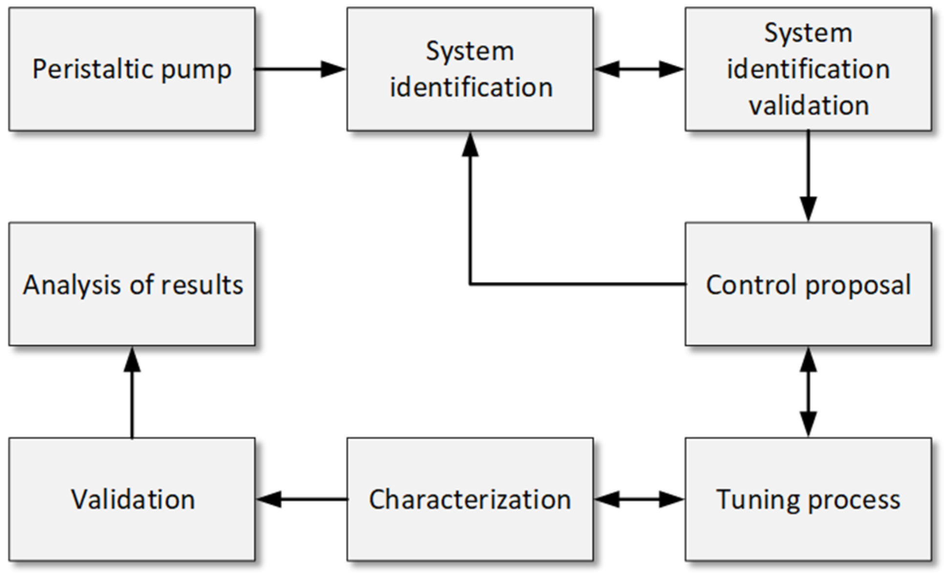
To address the objectives of this study, a comprehensive methodology was developed to identify, characterize, and control the peristaltic pump in a hemodialysis machine. The methodological process, as shown in Figure 1, highlights six stages: setting up communication between the pump, microcontroller, and LabVIEW; identifying the system; validating the transfer function; selecting the controller; and characterizing the system. These stages ensure the accuracy and repeatability of the pump’s performance under varying conditions.
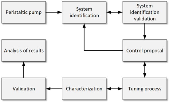
Figure 1.
Methodology flowchart for the identification, control, characterization, and validation of peristaltic pumps. Caption: Flowchart illustrating the steps followed in the study for the identification, control, characterization, and validation of peristaltic pumps in a hemodialysis machine. It includes the communication between the microcontroller and LabVIEW, system identification, controller selection, and system characterization under different operating conditions.
This methodology aims not only to identify and control the system but also to characterize it to establish the precise relationship between revolutions per minute (RPM) and volumetric flow rate (mL/min). It is expected that the P.I. controller will minimize flow fluctuations and achieve low RMSE values, demonstrating stability and accuracy under realistic conditions. Additionally, repeated measurements at different setpoints are anticipated to provide consistent data, highlighting the system’s ability to maintain uniform flow. The results will be compared to a commercial hemodialysis machine configured under identical conditions, allowing the developed system’s effectiveness to be evaluated against a commercial standard.
2.1. Peristaltic Pump
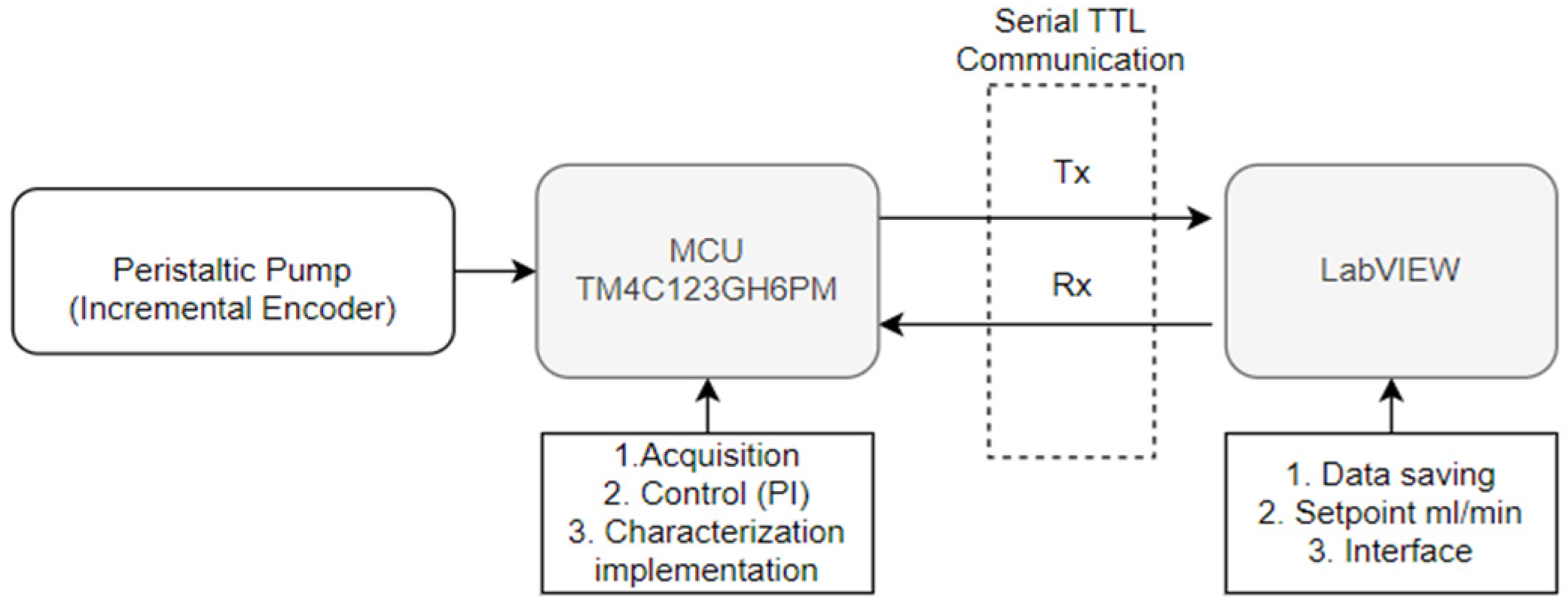
Figure 2 illustrates the automated control system for a peristaltic pump with an incremental encoder. The system consists of several interconnected components to enable data acquisition, control implementation, and user interaction. The TM4C123GH6PM microcontroller processes encoder data, regulates the pump’s PWM using a P.I. controller, and ensures proper system operation under varying conditions. Communication with LabVIEW is established through TTL serial transmission and reception (Tx/Rx) lines, with a 1 ms sampling time for rapid data updates and control adjustments. LabVIEW serves as the user interface, managing data storage, setpoint configuration in mL/min, and overall system interaction.
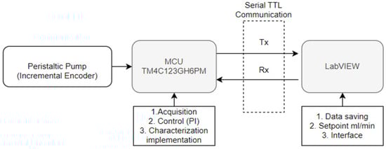
Figure 2.
Communication diagram for peristaltic pump with microcontroller and LabVIEW. Caption: Graphic representation of the automated control system including a TM4C123GH6PM microcontroller, an incremental encoder, and its integration with LabVIEW via TTL serial communication. The figure highlights the key elements for data acquisition and control of the peristaltic pump.
2.2. System Identification
System identification is a fundamental technique for modeling and controlling electric motors, especially D.C. motors, as it enables the creation of precise mathematical models from experimental data for efficient controller design. Methods like ARX, ARMAX (which includes a moving average term), and the non-linear least squares method are widely used [12,13]. Among these, the non-linear least squares method stands out for its ability to accurately estimate transfer function parameters in non-linear systems, even under noise and disturbances, making it ideal where linear methods are insufficient [14]. Its application has proven effective in optimizing robotic motion control and D.C. motor performance, showcasing its adaptability across systems with complex dynamics [15,16].
In light of the above considerations, it is imperative to convert the encoder pulses to revolutions per minute (RPM) to obtain the system’s response data. In order to achieve this, a Hall effect sensor and an integrated encoder within the peristaltic pump were employed. A tally was conducted to ascertain the number of pulses generated by the encoder throughout a complete revolution, with each instance of the Hall effect sensor issuing a signal being recorded. The result was a total of 45,800 pulses per revolution (PPR), which establishes the encoder’s resolution, as demonstrated by the following Equation (1):
At this stage, the estimation of revolutions per minute (RPM) is initiated. To this end, an interrupt on the TIVA microcontroller was employed to ascertain the number of pulses per millisecond (PPms), thereby facilitating enhanced precision in the estimation of RPM. The calculation is described in detail in Equation (2):
Given that the TIVA transmits the PPMS data at a rate of one sample per millisecond, this value is divided by 0.7633 to facilitate conversion to RPM.
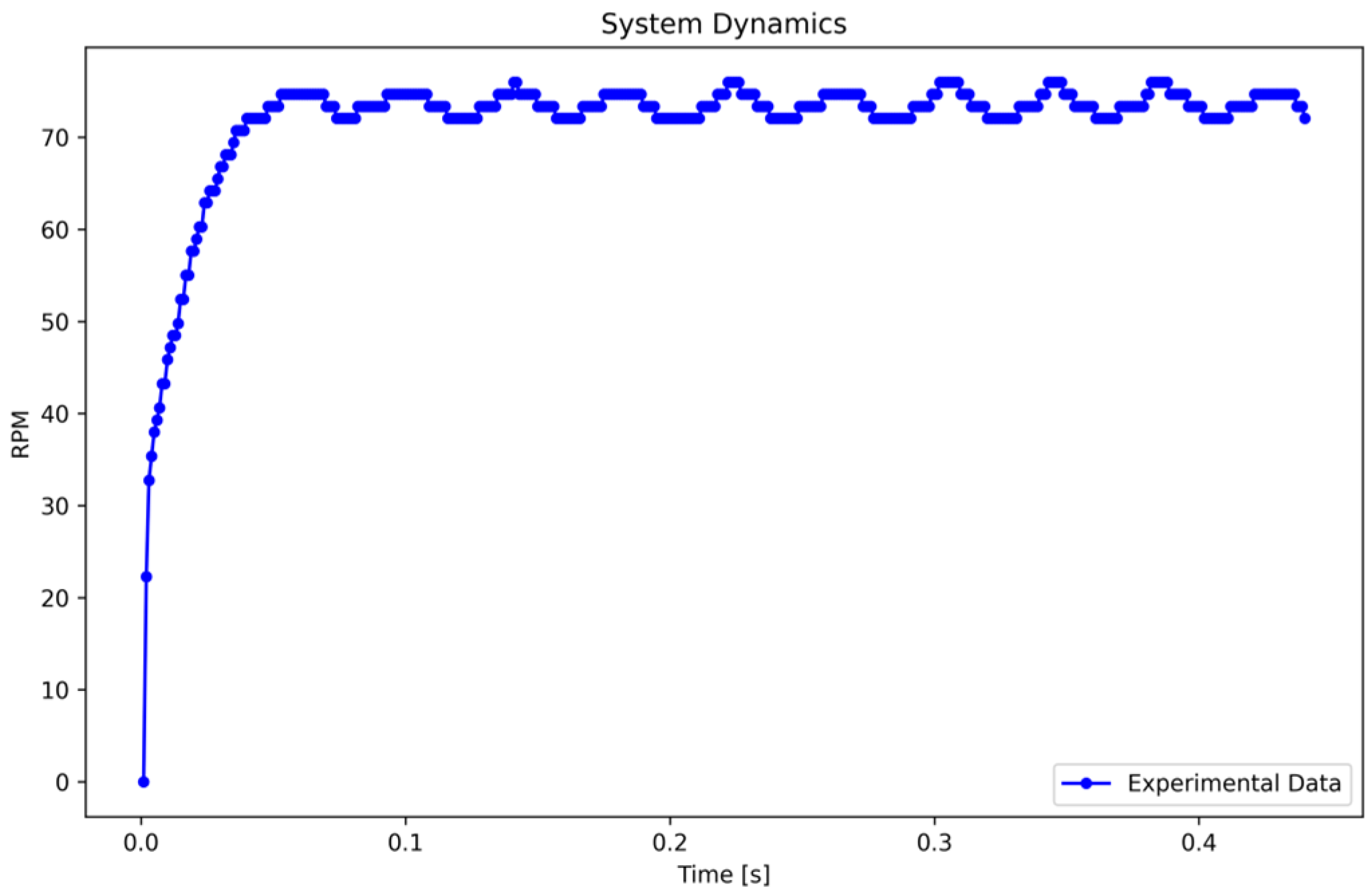
Subsequently, a step input of 24 V, equivalent to 100% of the input, is applied to the system. The RPM data are recorded at a rate of one sample per millisecond, resulting in the system response illustrated in Figure 3.
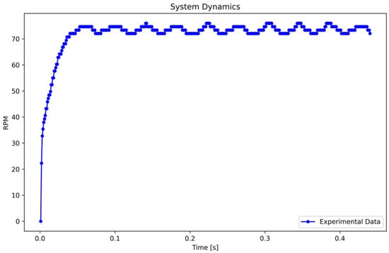
Figure 3.
System dynamics in response to a step input. Caption: System response to a 24 V step input, showing the inherent oscillations due to the dynamic characteristics of the peristaltic pump. Fluctuations between 72.05 and 74.67 RPM are attributed to transient response and system inertia.
The oscillations in Figure 3 result from the system’s inherent dynamics and transient response to a step input. These oscillations, caused by system inertia and variations in encoder pulses, fluctuate between 72.0524 and 74.6724 RPM. To determine the maximum amplitude representation, the mean value of data from 0.08 to 0.45 s was calculated, yielding 73.3284 RPM, which reflects the system’s steady-state behavior under dynamic conditions.
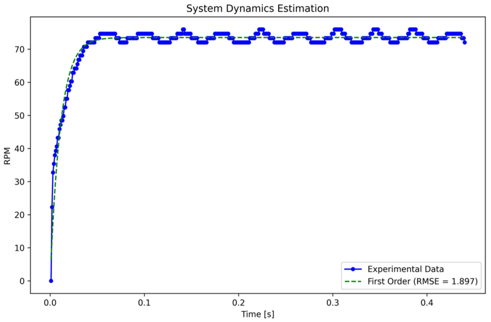
In order to estimate the transfer function of a system using sampled data, a curve-fitting process based on the non-linear least squares method was employed. This technique minimizes the residuals between observed and predicted data, ensuring accurate estimation of the transfer function parameters. In this instance, a first-order model was fitted to the experimental RPM data obtained over time, as this function most closely resembled the sampled data. The choice of the non-linear least squares method is grounded in its ability to model non-linear systems with high accuracy, minimizing the impact of noise and experimental disturbances. This approach has proven effective in complex dynamic systems, such as DC motors and peristaltic pumps, particularly in medical control applications, as reported in previous studies [14,15]. By employing this method, the transfer function parameters are estimated precisely, ensuring that the dynamic behavior of the peristaltic pump is accurately captured, even under varying experimental conditions.
The first-order transfer function in the Laplace domain is defined as shown in Equation (3):
The objective of the non-linear least squares method is to minimize the sum of the squares of the differences between the observed values and the values predicted by the model. The objective function to be minimized is defined as follows:
where represents observed RPM values at time , while denotes the predicted value as calculated by the model. The latter employs the parameters to describe the first-order transfer function. Finally, signifies the time at which each respective sample was taken. The fitting process is implemented using the Levenberg–Marquardt algorithm [17], which combines the Gauss-Newton and gradient descent methods to estimate the optimal parameters . Following the completion of the fitting process, the transfer function is expressed as illustrated in Equation (5):
The estimated function provides a satisfactory approximation, as evidenced by the fact that when we multiply , the result represents 98.2% of the maximum amplitude. Nevertheless, the accuracy of the transfer function is evaluated using the root mean squared error (RMSE), as detailed in Equation (6):
where are the values predicted by the model, resulting in an estimation error of 1.897 RPM, as illustrated in Figure 4.
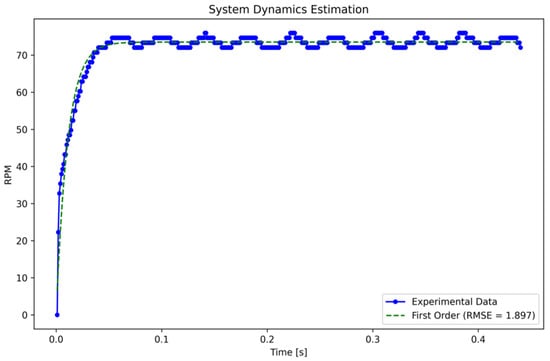
Figure 4.
First-order system identification. Caption: Adjustment of the first-order transfer function using experimental data obtained using the non-linear least squares method. The function accurately represents the system dynamics with an RMSE of 1.897 RPM.
2.3. Auxiliary Methodologies for System Approximation Verification
The efficacy of the proposed first-order system approximation about the sampled data is evaluated using the functions defined in the following equations, which employ the optimization methods proposed in [18,19,20,21]. The aforementioned analysis yielded the comprehensive evaluation detailed in Table 1

Table 1.
Percentage of approximation error: data vs. proposed first-order plant.
A number of tools are available for the qualitative verification and validation of control systems. This section presents four approaches to verification through the calculation of definite integrals, as illustrated in the following equations. The optimization functions are classified into four categories. The Integral Absolute Error (IAE), the Integral Squared Error (ISE), the Integral Time-weighted Absolute Error (ITAE), and the Integral Time-weighted Squared Error (ITSE) are integral-based error metrics.
The Integral Absolute Error (IAE) [21] is a metric utilized in control systems to assess a controller’s performance based on the accumulated error over time. It is defined as the integral of the absolute value of the error between the reference signal and the system output signal, as expressed in Equation (7). In contrast to metrics such as the Integral Squared Error (ISE), which assigns greater significance to more significant errors, the IAE assigns equal weight to all errors, rendering it a valuable tool for minimizing the overall system error without unduly emphasizing more significant errors.
The Integral of Squared Error (ISE) [22,23] is a performance metric employed in analyzing control systems to quantify the accumulated error over time, emphasizing more significant errors. The Integral of Squared Error (ISE) is the integral of the square of the error between the reference signal and the system output signal, as expressed in Equation (8). The ISE assigns a greater penalty to more significant errors due to the use of the squared error, making it particularly useful in applications where the minimization of significant deviations from the reference signal is desired. This metric is frequently employed in the design and tuning of controllers to optimize system performance and enhance stability.
The Integral of Time-weighted Absolute Error (ITAE) [18,19] is a performance metric utilized in the design of control systems for evaluating error as a function of time. The Integral of Time-weighted Absolute Error (ITAE) is defined as the integral of the product of time and the absolute value of the error between the reference signal and the system output signal, as illustrated in Equation (9). The ITAE assigns greater significance to errors that manifest later, thereby imposing a more substantial penalty on prolonged errors. This encourages a more expeditious correction of errors, rendering this metric particularly useful in applications where both accuracy and rapid system response are desired.
The Integral of Time-weighted Squared Error (ITSE) [22,23] is a performance metric utilized in the analysis of control systems, wherein the squared error is weighted as a function of time. The Integral of Time-weighted Squared Error (ITSE) is defined as the integral of the product of time and the square of the error between the reference signal and the system output signal, as illustrated in Equation (10). The ITSE assigns more significant penalties to errors that persist over more extended periods. This time-weighted approach encourages rapid responses and mitigates long-term errors, rendering it especially beneficial in systems where the objective is to diminish sustained errors over time to enhance both precision and stability.
The values in Table 1 indicate a minimal average approximation error, substantiating the assertion that the first-order system’s approximation to the experimental response data are acceptable and optimal. The application of the ISE methodology yielded an approximation error parameter of 3.4670%, which is higher than that observed in the other methodologies. Nevertheless, this value only significantly affects the conclusion that the proposed first-order system is optimal. In light of the findings from the preceding methodologies, it can be concluded that the proposed first-order system is a suitable means of analyzing responses in simulated computational systems.
2.4. Controller Design
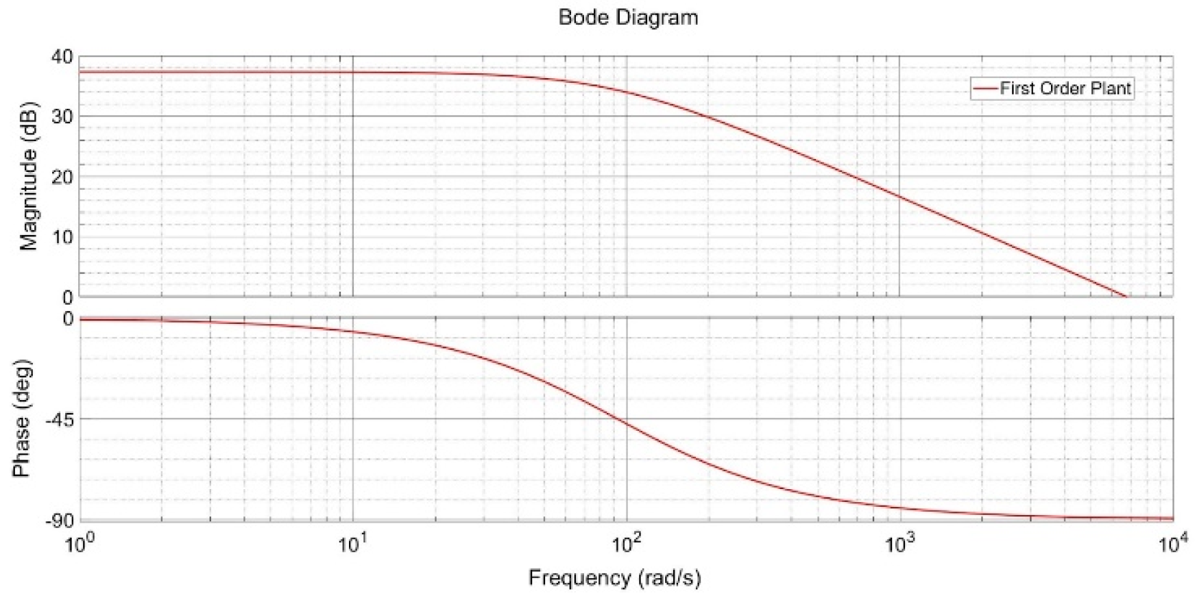
Classical procedures in automatic control are based on assumptions about the plant and the desired outcome. Furthermore, these procedures aim to obtain specific characteristics of the process, either analytically and/or visually. Subsequently, this knowledge is employed in the selection of the controller configuration. These strategies are appropriate for the preliminary phase, as they are computationally rapid and straightforward to implement. Nevertheless, attaining the anticipated outcomes from the controller configuration is not always feasible due to the underlying assumptions. In this article, the data obtained from experimentation are evaluated in the frequency domain. The Bode diagram is handy for elucidating how a system responds to disparate input frequencies. The magnitude plot presents the system’s gain as a function of frequency on a logarithmic scale, while the phase plot shows the corresponding phase shift.
In systems where the magnitude decreases at high frequencies, this indicates that the expected response acts as a low-pass filter, which is beneficial for attenuating high-frequency noise or disturbances. However, this behavior also indicates the potential for inadequate compensation at low frequencies, which can result in steady-state errors if appropriate integrative action is not introduced, as previously discussed in [18].
In such instances, the P.I. controller regulates the system’s behavior by addressing immediate errors through its proportional term and eliminating steady-state errors with its integral term.
As shown in Figure 5, the Bode plot highlights the need for additional low-frequency compensation, addressed by the introduction of the P.I. controller. This controller improves the system’s phase margin and stability, ensuring reliable performance. The enhanced stability is particularly significant for practical applications, where maintaining system reliability under dynamic conditions is critical.
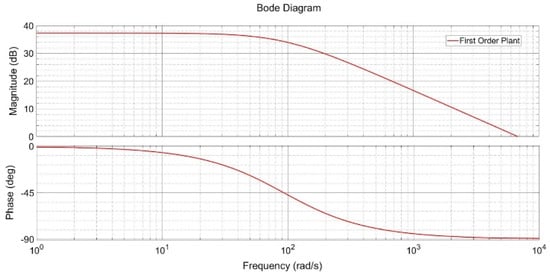
Figure 5.
Bode plot of the proposed first-order plant. Caption: Frequency response analysis of the identified system, showing magnitude and phase at different frequencies. This analysis supported the selection of the P.I. controller to improve stability and reduce steady-state error.
2.5. Gain Estimation
The MATLAB 2014 software provides a tool for fine-tuning PID controllers in PID tuners based on optimization techniques and response, employing Ziegler–Nichols and frequency response methods [24]. The process, designated the PID tuner, adheres to a prescribed sequence of steps for its preliminary tuning, which encompasses the following:
- System modeling: The application can accept a transfer function as an input or estimate it. The previously estimated transfer function (see Equation (5)) was input in the present case;
- The initial parameters of the PID controller are calculated by MATLAB using frequency-based techniques based on the principles set forth by the Frequency Response Theorem and Ziegler-Nichols. This approach permits the identification of an initial configuration that offers an optimal equilibrium between stability, response speed, and damping;
- The objective of performance-based optimization is to achieve optimal performance. Once the initial PID parameter values have been obtained, the PID Tuner employs optimization algorithms to fine-tune the Kp, Ki, and Kd parameters;
- The following performance criteria will be considered: In the preceding step of the optimization process, the application also considers performance criteria, including minimizing overshoot, settling time, response speed, and steady-state error;
- Controller validation: The tuned controller is subsequently validated through simulations to guarantee that it fulfills the design specifications, including stability and the desired performance regarding response time and frequency analysis.
In accordance with the aforementioned methodology, the PID Tuner facilitates the acquisition of the preliminary tuning parameters, for example, for a PI-type controller. In light of the results mentioned above derived from the first-order plant approximation, the proportional gain and the integral gain were estimated.
The use of a P.I. controller is supported by its ability to correct steady-state errors and improve system stability. Previous studies have demonstrated its effectiveness in peristaltic pumps, emphasizing its capability to reduce fluctuations in high-precision applications such as hemodialysis [25,26]. In this case, the inclusion of the integral term ensures adequate control even under variable load conditions, while the proportional term responds quickly to transient errors, optimizing the overall system performance. This combination makes the P.I. controller particularly suitable for maintaining precise flow rates in medical applications.
The controller incorporates the constants, and the peristaltic pump is characterized by establishing a correlation between the revolutions per minute (RPM) and the delivered volume and mass. This methodology is delineated in the following section.
2.6. Statistical Analysis and Validation of Results
This section describes the statistical approach adopted to validate the accuracy and reliability of the results obtained in the study. This analysis aims to provide a quantitative basis that supports the superiority of the developed system compared to a commercial hemodialysis machine and to evaluate the performance of the RPM estimates against the flow values in mL/min.
To evaluate the system’s performance and the accuracy of the characterization functions that relate RPM to flow values in mL/min, three main metrics were employed. The RMSE was used to measure the magnitude of the estimation error, especially penalizing larger errors. The average error was used to evaluate the overall system performance in relation to the target values, while the standard deviation quantified the variability in the estimates, providing a measure of the system’s stability.
Another important metric was the calculation of precision ratios, defined as the relationship between the measured flow and the desired flow. These ratios evaluate the system’s efficiency in maintaining flows close to the target, a critical characteristic in clinical applications where any deviation can impact patient safety.
To determine whether the observed differences between the developed system and the commercial machine were statistically significant, a paired t-test focused on the errors was conducted. This test compares the average errors of both systems under the same experimental conditions, providing formal validation of the proposed system’s superiority. Error measurements were collected for both the developed system and the commercial machine across the same flow ranges (20–600 mL/min), which will be detailed later Each flow setpoint included repeated measurements to ensure robustness and consistency in the results. For each flow range, the absolute error of the developed system was subtracted from the absolute error of the commercial machine to compute the error differences. These differences served as the basis for the paired t-test, which evaluated whether the mean of these differences was significantly different from zero.
The analysis ensured accurate computation of the t-value and p-value. A p-value below 0.05 was considered evidence of statistically significant differences in the errors, validating the developed system’s improved performance.
Based on preliminary results, it is anticipated that the developed system will show significantly lower errors than the commercial machine, supporting its superior precision. Additionally, the ratios are expected to exhibit consistent values close to the ideal in both systems, highlighting their capability to maintain precise flows. This statistical approach complements the experimental measurements and reinforces confidence in the obtained results.
3. Analysis of Results
This section analyzes the results obtained for the proposed control, system characterization, and validation. Errors relative to the controller setpoint are examined, along with the outcomes of the metrics used for system identification. Additionally, the characterization data are evaluated, including the selection of the estimated function. This selection was based on a comparison of experimental data across a polynomial model, a potential model, and a linear model, with the polynomial function ultimately proving to be the most accurate. The analysis is further supported by validation against a commercial hemodialysis machine using volume measurements, ensuring the accuracy and reliability of the characterization performed.
3.1. Control System
In this study, a P.I. controller was tuned based on experimental data obtained from a physical plant subjected to a unit step input. From the samples collected, the first-order transfer function characteristic of the system was identified, which describes the dynamics of the proposed plant. This mathematical model was validated using different error optimization methods, which allowed a precise evaluation of the model fidelity with respect to the experimental data.
The error calculation methods used for model validation included IAE, ISE, ITAE, and ITSE. These performance metrics provided a comprehensive assessment of the fit between the simulated response of the modeled system and the actual data obtained from the physical plant. The integration of these metrics helped to identify and validate the magnitude of the system error.
The validation results indicated an excellent approximation between the response of the proposed first-order system and the sampled data, with a residual error close to zero. This result highlights the accuracy of the first-order model in capturing the dynamics of the system, suggesting that it is an optimal representation for the analysis and design of control strategies. The low magnitude of the accumulated error over time validates the robustness of the applied methodological approach and supports using the modeled plant as a basis for controller development.
The frequency analysis of the system was performed using a Bode diagram, which allows an evaluation of the system’s dynamic behavior in the frequency domain. The Bode diagram showed a decreasing magnitude at high frequencies and a phase indicating system stability within the desired operating range. Based on these results, it was determined that implementing a P.I. controller would be the optimal alternative for system control. The P.I. controller was chosen for its ability to correct steady-state errors without compromising system robustness while significantly improving stability and effective disturbance rejection. The tuning of the P.I. controller was carried out, taking into account the plant characteristics identified by the Bode analysis and the MATLAB tool, ensuring optimal performance under the established operating conditions.
The automatic optimization technique provided by MATLAB’s PID Tuner tool was used to tune the P.I. controller. This automatic tuning tool efficiently adjusted the controller parameters ( and ) to optimize the control system’s performance under the specified operating conditions. The parameters obtained through this technique were then applied to the physical plant to verify its performance in a real experimental environment. The experimental results confirmed the effectiveness of the automatic tuning and demonstrated excellent system behavior under P.I. control.
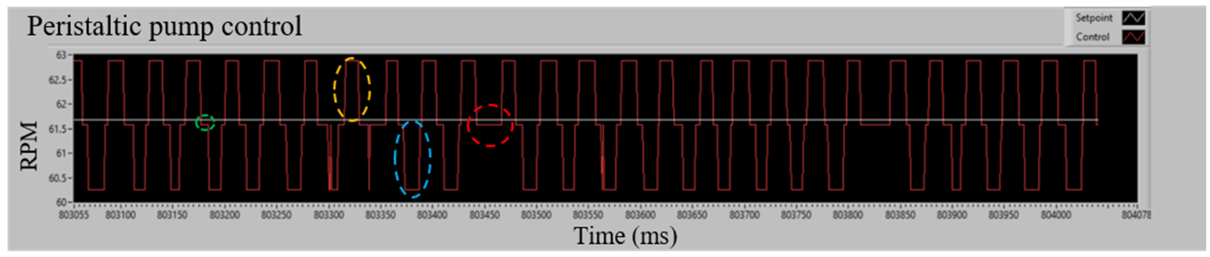
Figure 6 shows the steady-state behavior of the pump under P.I. control at a setpoint of 61.57 RPM. The system exhibits symmetrical deviations of approximately ±2 RPM due to the compression and release mechanism of the rollers. Positive deviations occur when a roller stops applying pressure to the hose (yellow dashed circle), while negative deviations are generated when the roller applies pressure to restart the process (blue dashed circle). These fluctuations are controlled by the system to maintain stability.
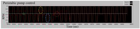
Figure 6.
PI control in steady state applied to a peristaltic pump. Caption: Variations in pump behavior under P.I. control at a setpoint of 61.57 RPM. The dashed circles highlight key points in the roller compression cycle, including deviations, stabilization phases, and controller adjustments to maintain system stability.
The green dashed circle indicates the center of the deviations, where all the rollers exert pressure on the hose and maintain a constant speed close to the setpoint. The red dashed circle marks the moments when the controller manages to reduce the negative deviations. Considering all the tests carried out for the characterization, as shown in Table 2, the RMSE of the speed deviations concerning the setpoint is calculated, which gives a value of 1.687 RPM.
Table 2.
Flow rate characterization in mL/min vs. RPM.
3.2. Characterization
Characterizing peristaltic pumps is essential for optimizing performance and ensuring flow accuracy, particularly in applications requiring sterile handling, such as hemodialysis [27,28]. These pumps operate by compressing and decompressing a flexible tube, minimizing contamination risk [2]. However, factors such as fluid-tubing interactions, influenced by properties like elasticity and viscosity, directly affect flow dynamics and accuracy [29]. Nonlinearities, such as oscillations caused by roller separation during operation, contribute to flow variability and performance reduction [30]. Similarly, non-Newtonian fluids, like synthetic blood, complicate flow dynamics due to shear-dependent viscosity and memory effects [25,31]. Proper characterization accounting for these factors ensures realistic flow rate estimations [26].
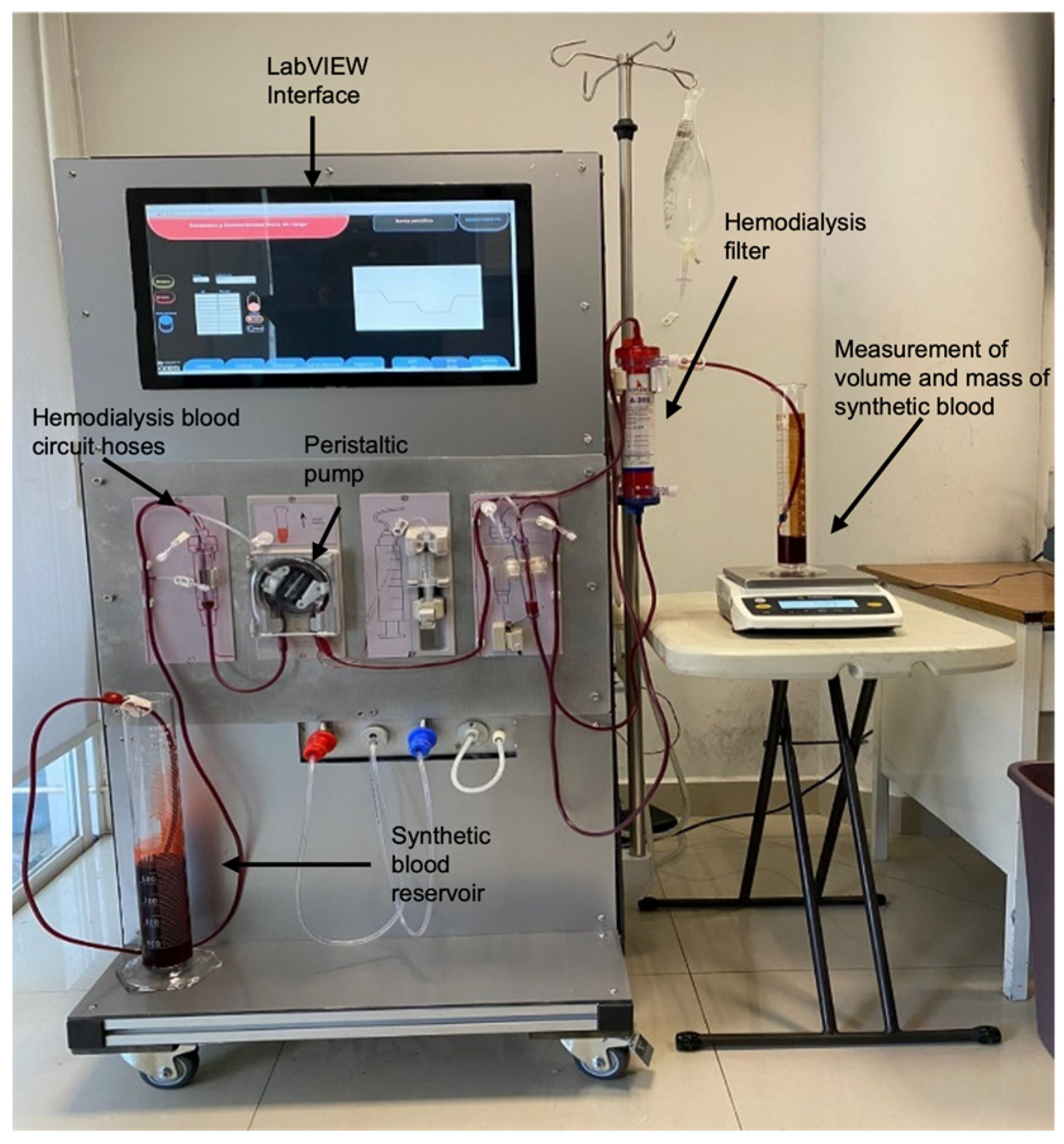
This study characterizes a peristaltic pump over a flow range from 1.5 RPM, where system inertia is overcome, to 73 RPM, the maximum operating limit. The target flow rates include 20, 100, 200, 300, 400, 500, 600, 700, and 730 mL/min, as summarized in Table 2. The experimental setup (Figure 7) is designed to enable a robust evaluation of the developed system’s performance. The setup integrates a peristaltic pump controlled via a LabVIEW interface, synthetic blood with clinically representative viscosity, and a hemodialysis filter to replicate real operational conditions. The LabVIEW interface synchronizes the pump’s operation with real-time flow monitoring, allowing precise adjustments to ensure consistent fluid transport through the patient circuit hoses. Volume and mass measurements are recorded using graduated cylinders and a Sartorius weight scale, ensuring precise flow characterization.
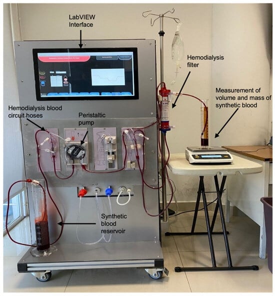
Figure 7.
Experimental setup for system characterization and validation. Caption: The system consists of a peristaltic pump controlled by a LabVIEW interface, connected to hemodialysis blood circuit hoses, and a synthetic blood reservoir. Synthetic blood flows through a hemodialysis filter to simulate real treatment conditions. Volume and mass measurements are recorded using graduated cylinders and a Sartorius weight scale to validate flow accuracy and stability. The setup replicates clinical conditions by integrating all components required for precise flow control, enabling characterization and validation of the developed control system under realistic operational scenarios. Note: Red dye was added only to visualize the synthetic blood.
Once the experimental setup was complete, the patient circuit tubing was entirely filled with fluid to ensure no air remained in the system. The procedure began by setting a pump controller setpoint of 1.5 RPM, allowing the system to stabilize before placing the tubing into a graduated cylinder for timed measurements. The pump was kept running continuously during all repetitions to maintain flow consistency and avoid resetting the roller position, which could introduce variability.
Flow rate calculations were derived by dividing the measured volume and mass by elapsed time. Measurement durations varied according to setpoint and cylinder capacity: 3 min for volumes of 20–300 mL, 2 min for 400–500 mL, and 1 min for 600–730 mL. To ensure accuracy and reliability, ten repetitions were conducted for each target flow rate. This methodology reduced variability, identified anomalies, and provided robust RMSE calculations, as shown in Table 2 [32,33].
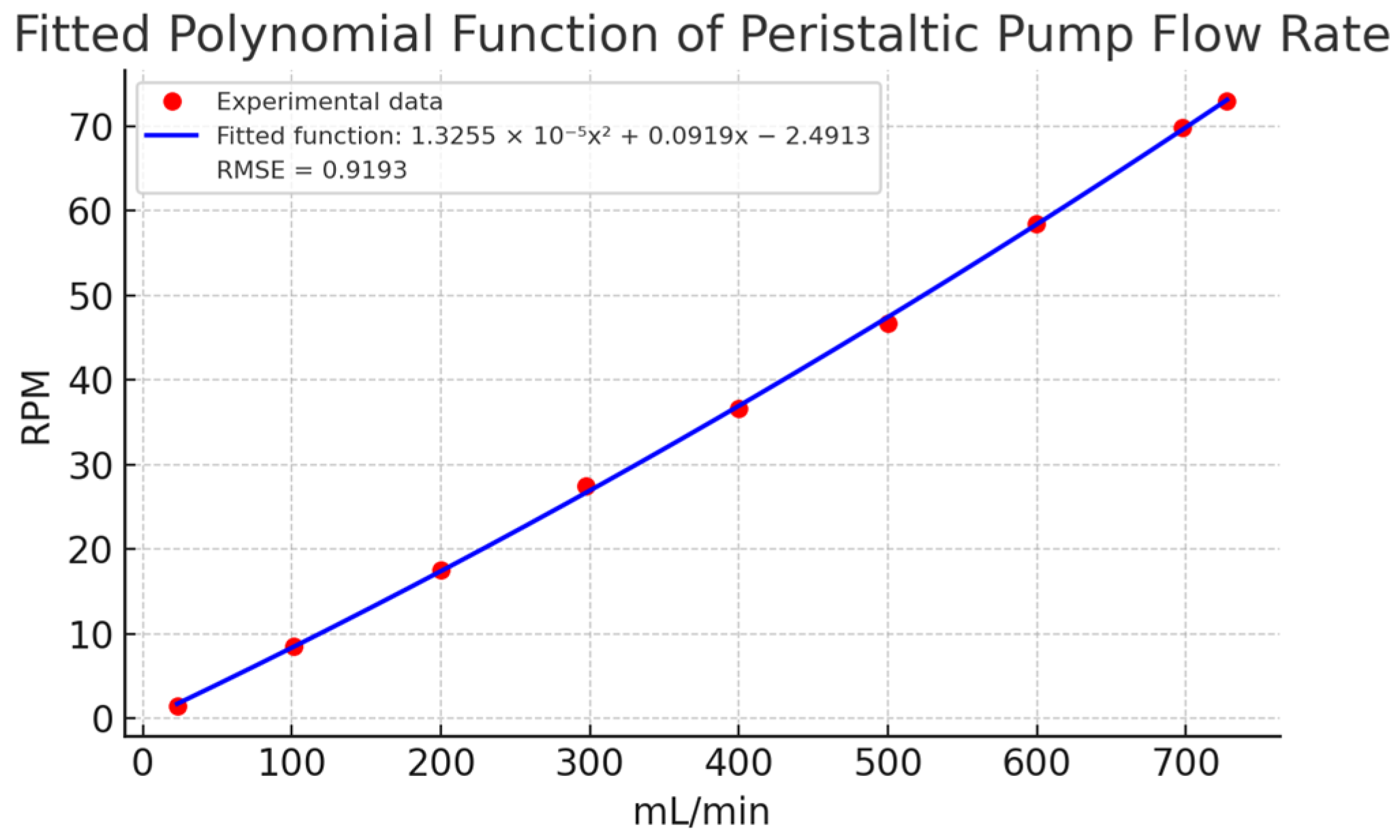
The relationship between RPM and flow rate (mL/min) was determined by averaging the ten replicates for each setpoint and plotting the results. Figure 8 illustrates the fitted polynomial function, which provided the best experimental fit with an RMSE of 0.9193 mL/min. This function was estimated using the non-linear least squares method, as detailed in Section 3.3 Validation. The polynomial model showed high accuracy in describing the relationship between RPM and flow, with minimal deviation between predicted and observed values.
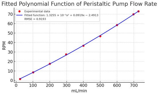
Figure 8.
Fitted polynomial function of experimental data of peristaltic pump flow rate. Caption: Relationship between revolutions per minute (RPM) and volumetric flow rate (mL/min) based on experimental data. The polynomial model provides the best fit with an RMSE of 0.9193 mL/min.
Table 2 highlights the statistical parameters for each setpoint, including average flow rate, standard deviation, and RMSE. The data indicate that the control system effectively maintains target flow rates with minimal variability. For example, at a target of 100 mL/min, the standard deviation was only 0.45 mL/min, reflecting high system accuracy. However, at higher flow rates, such as 600 mL/min, the standard deviation increased to 0.60 mL/min, consistent with prior studies that show greater variability at higher RPMs [25,30,31]. Despite this, the controller maintained a maximum error of only 1.897 RPM across all setpoints.
The RMSE, measuring deviations between observed and target values, was relatively low across the range. For instance, the RMSE at 200 mL/min was zero, highlighting excellent accuracy at this point. However, at higher flow rates, such as 700 mL/min and 730 mL/min, the RMSE increased, reflecting the greater challenges in maintaining consistency at elevated speeds. These findings are consistent with previous research indicating that fluid dynamics and tubing friction introduce variability at higher RPMs [29,30,31].
The P.I. controller demonstrated strong performance, achieving minimal steady-state error and excellent repeatability across all tests. This indicates its suitability for precise control applications, particularly those requiring consistent and accurate flow regulation.
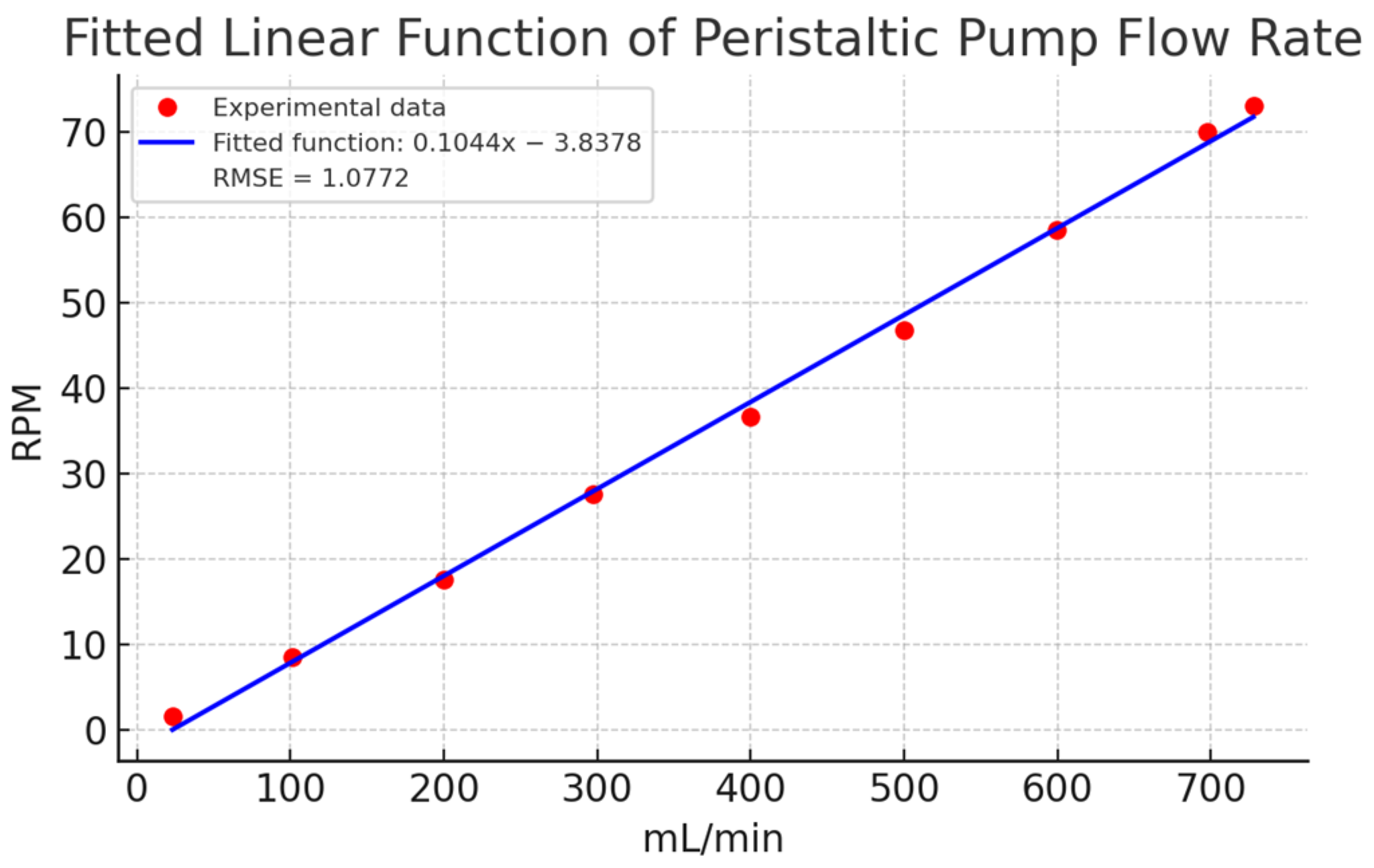
Finally, Figure 9 compares a linear estimation with the experimental data. The linear model showed deviations exceeding 15 mL/min in key points (e.g., 100, 400, 500, and 700 mL/min), confirming the need for a non-linear approach. The fitted polynomial function, with its small quadratic coefficient (1.3255 × 10⁻⁵), closely approximates a linear relationship but provides better accuracy. These results affirm that a non-linear model is more appropriate for describing the relationship between flow and RPM in peristaltic pumps.
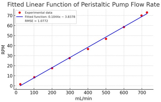
Figure 9.
Estimation of a linear function for the experimental characterization data in Table 2. Caption: Comparison of the linear estimation with experimental data, showing significant deviations at key points. This highlights the need for a non-linear model for better representation.
3.3. Validation
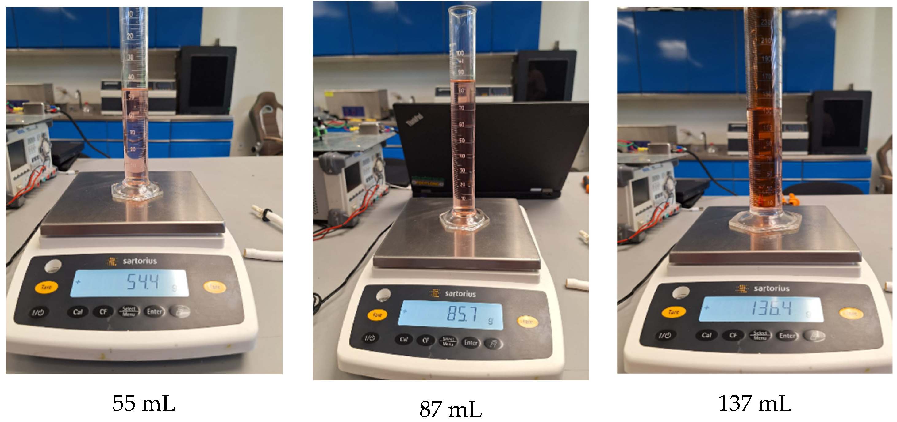
Figure 10 shows nine random tests performed for in situ characterization and control. Each sub-image shows the applied setpoint at the bottom, with the corresponding mass and volume measurements displayed within the image. Both the volume and mass measurements are close to the target values. The images also include the results of the tests using the polynomial function, which demonstrated the best performance in experimental trials. Detailed measurements from these tests are presented in Table 3.

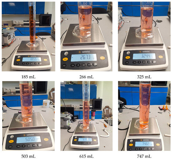
Figure 10.
Characterization and control test with volume and mass measurement. Caption: Results of nine random in situ characterization tests. Includes mass and volume measurements close to target values, validating the accuracy of the polynomial model in experimental applications. Note: Red dye was added only to visualize the synthetic blood.
Table 3.
Flow rate characterization in mL/min vs. RPM.
Table 3 presents a detailed analysis of the accuracy and control of the measurement system over different flow ranges, from 20 to 100 mL/min to 700–730 mL/min. For each range, both the target values and the actual measurements obtained using a weight scale and graduated cylinder were recorded. This approach allows the system’s accuracy to be evaluated by comparing the measurements to the target values. It is important to note that the values tested were randomly selected and not the same as those used for characterization to assess generalization.
The analysis of the measurement errors shows that the deviations between the actual measurements and the target values are generally minor, indicating a high level of accuracy in the system’s performance. In the case of the weight scale, the errors range between 0.06 and 8.8 g, showing that the mass measurements are very close to the setpoints. Similarly, the errors observed when comparing the setpoints with the graduated cylinder data range from 0 to 7 mL, reflecting remarkable consistency in the volumetric measurements.
In addition, the calculated ratios between the mass per minute (g/min) and volume per minute (mL/min) measurements are close to 1 in most cases. This indicates that the conversions between mass and volume are consistent and accurate across the different flow ranges. The average ratios for g/min and mL/min are 1.0013 and 0.9999, respectively, indicating excellent system control. The deviation observed in the ratio complements of 0.1314% for g/min and 0.001% for mL/min further supports the idea that the system is robust and capable of maintaining consistent accuracy.
When examining the error ranges across different flow rates, it is evident that the system maintains high precision even at the lowest and highest flow ranges. This suggests that the measurement system is highly reliable across its full operational spectrum, a crucial attribute for applications requiring both low and high flow rates. Additionally, the low average errors and tight ratios further support the system’s suitability for environments where precision and repeatability are critical, such as in hemodialysis treatments.
In summary, the analysis in Table 3 shows that the measurement system is highly reliable, with minimal errors and ratios close to ideal values. This confirms that both mass and volume measurements are close to the target values, providing confidence in the accuracy and repeatability of the system used, which is essential for ensuring consistent and safe performance in sensitive applications.
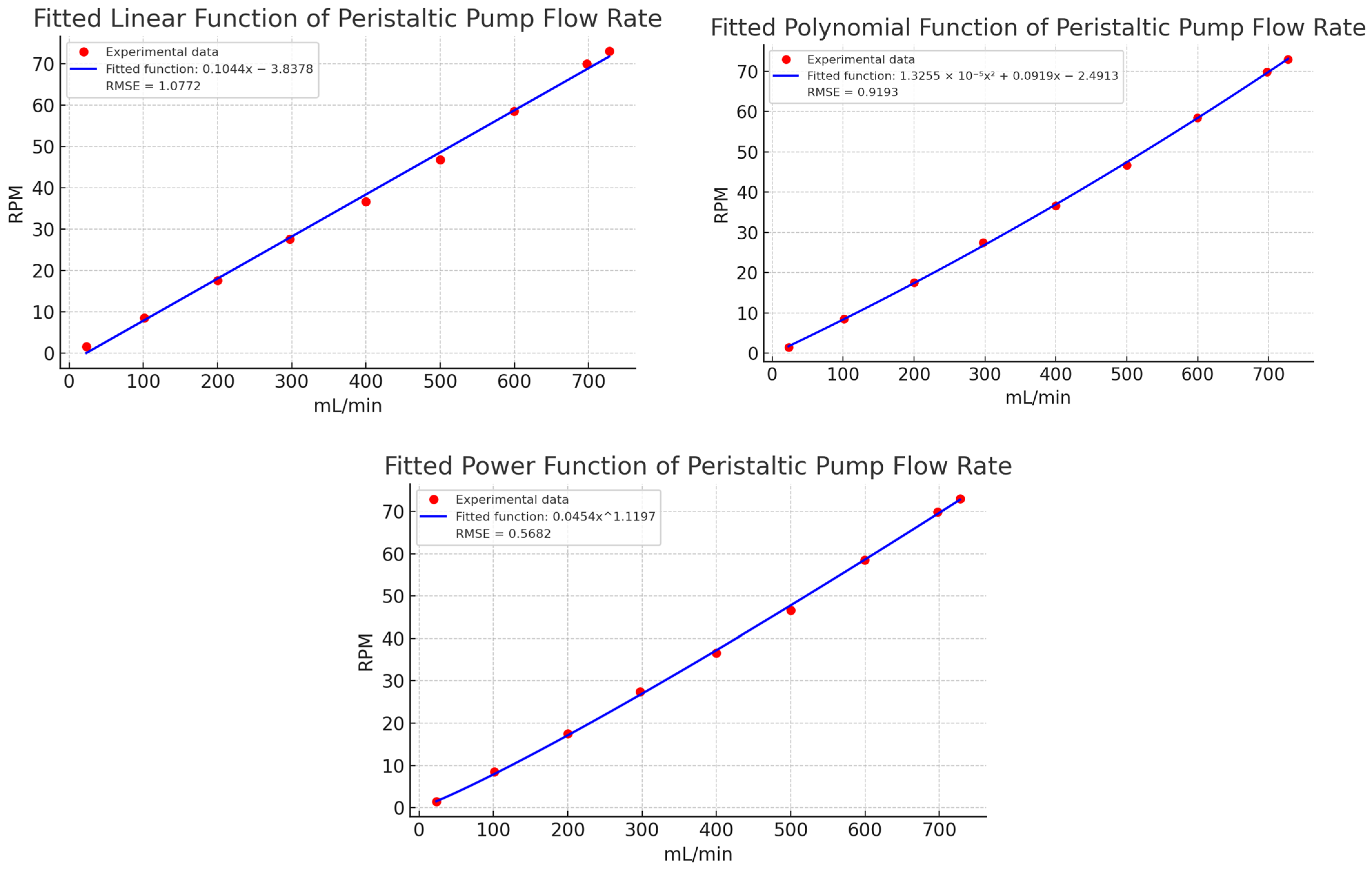
To validate the polynomial function’s superior accuracy in describing the peristaltic pump’s behavior, Table 4 compares volumetric flow results from 32 tests conducted at the same setpoints as in Table 3. This comparison includes the potential, linear, and polynomial estimations shown in Figure 11, highlighting the differences in accuracy between the models and identifying the one that best aligns with the target values.
Table 4.
Flow rate comparison between lineal and non-lineal estimation.
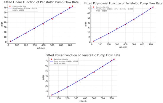
Figure 11.
Linear, potential, and polynomial estimation of the experimental characterization data in Table 2. Caption: Comparison of linear, polynomial, and power function estimations of experimental data for peristaltic pump flow rate. The polynomial model demonstrates the best fit with minimal error, highlighting the limitations of linear and power functions in capturing the system’s dynamics.
A comparative analysis of the flow estimation methods in Table 4 reveals that polynomial estimation provides superior precision and consistency across all flow ranges, as highlighted in bold within the table. This method maintains a consistently low error level, often below 1 mL/min and, in many cases, as low as 0 mL/min, indicating that it effectively captures the non-linear relationship between speed and flow (mL/min). While potential estimation reduces errors more effectively than the linear method, it shows more variability, with errors ranging from 0 to 26 mL/min depending on the setpoint. This suggests that potential estimation lacks the precision of the polynomial approach. In contrast, linear estimation shows the highest error values, reaching up to 37 mL/min, reflecting its limitations in accurately modeling the non-linearities in the speed-flow relationship.
The relationship between actual and estimated values clearly supports the accuracy of the polynomial method. Across most setpoints, particularly within the 20–100 mL/min and 100–200 mL/min ranges, polynomial estimation ratios remain close to 1, indicating high consistency in predicting actual values. While potential estimation ratios are closer to 1 than those from linear estimation, they exhibit larger deviations at higher flow rates, fluctuating between 1.0067 and 1.0369, indicating moderate accuracy. In contrast, linear estimation ratios are significantly higher, such as 1.5865 and 1.2102 in lower ranges (20–100 mL/min). Although these ratios stabilize closer to 1 at higher ranges, this variability suggests that linear estimation may not be ideal for accurately modeling this dataset.
The efficacy of each estimation technique is contingent upon the flow range in question. In the low flow range (20–100 mL/min), polynomial estimation demonstrates near-perfect accuracy, exhibiting consistently lower errors than both linear and potential methods. As flow rates exceed 500 mL/min, all three estimation techniques demonstrate enhanced ratio consistency. Nevertheless, polynomial estimation remains the most accurate, followed by potential estimation, while linear estimation is the least accurate, particularly at the highest flow rates (600–730 mL/min). In this upper range, polynomial estimation exhibits the lowest error rates, demonstrating robust performance across the entire data series.
While the RMSE values for all estimation methods illustrated in Figure 11 are relatively low, even minor discrepancies can have a considerable impact on experimental outcomes. Minor discrepancies in accuracy can result in cumulative errors in flow rate predictions in real-world conditions. The lower RMSE of polynomial estimation in comparison to linear and potential methods demonstrates its superior capacity to capture subtle non-linearities in the speed-flow relationship. This advantage is of particular importance in practical settings, where even minor errors can have a significant impact on flow regulation, particularly in applications that require precise control. Therefore, while all methods perform well theoretically, the slight RMSE advantage of polynomial estimation becomes important in experimental conditions. In light of the aforementioned considerations and the specific results presented in Table 4, the polynomial function is deemed to be the optimal method.
In order to validate the volumetric flow of our control and characterization proposal, and once the appropriate function relating RPM to mL/min was selected, a comparison was made with the volumetric flow of a commercial hemodialysis machine used as a reference. The commercial machine was configured under the same conditions as ours, using a blood circuit of the same diameter and brand, as well as the same filter. Twenty-four different setpoints were measured within a range of 20 to 600 mL/min, which aligns with the operating range of the reference machine. Additionally, the machine’s resolution of 5 mL was maintained. For each measurement, the average error (calculated as the difference between the setpoint and the measured value) and the ratio (representing the proportion between the setpoint and the measured value) were calculated, as shown in Table 5.
Table 5.
Comparison between the volumetric flow of our proposal and the commercial hemodialysis machine.
A review of Table 5 reveals that the reference hemodialysis machine exhibits an average error of approximately 8.9929 mL/min, whereas our control system demonstrates a lower average error of 4.0000 mL/min. This discrepancy serves to illustrate the enhanced precision of our control system in maintaining the specified flow rate across the tested range. Specifically, the reference machine exhibits a range of errors between 4 and 20 mL/min, with larger deviations observed at higher flow rates. In contrast, our control system demonstrates a consistent ability to limit deviations to below 10 mL/min at the majority of set points.
With regard to the ratio values, the control system once again demonstrates superior performance in comparison to the reference machine. The commercial machine has an average ratio of approximately 0.9723, while the control system achieves a ratio closer to 0.9947, approaching the ideal value of 1. This closer alignment demonstrates that the control system is more effective at maintaining the setpoint flow rate, particularly at higher flows where precise control is essential. Moreover, while the reference machine exhibits ratio values as low as 0.9270 at lower flow rates and slight excesses at specific higher set points (e.g., 1.0345 at 300 mL/min), our control system maintains a consistent ratio close to 1:1 across all tested points.
Furthermore, the complement of the ratio values (2.6582% for the reference machine vs. 0.5296% for our control system) provides additional confirmation that our system achieves significantly higher accuracy and stability, with deviations that are nearly five times lower than those of the reference machine. These findings indicate that our control system may offer a more reliable and consistent solution for hemodialysis, maintaining precise flow rates that are critical for patient safety and treatment effectiveness.
It is also of significance to consider the system’s response across a range of flow rates, with particular attention paid to its performance at the upper and lower limits of the operational range. The data indicates that the control system exhibits high accuracy and low deviation at both low and high flow rates, thereby demonstrating robust performance across the entire range. This characteristic is of particular importance in applications such as hemodialysis, where the system must operate in a reliable and consistent manner, even when subjected to fine adjustments at lower flow rates, and must also be capable of handling higher flow rates without significant deviation. The consistency in the performance of our control system across these ranges serves to highlight both its adaptability and reliability, rendering it particularly well suited to scenarios that require stable performance across varying conditions.
Moreover, the effectiveness of the controller in experimental settings is yet to be determined. The control system displays rapid responsiveness to setpoints, thereby maintaining stability even in the presence of potential fluctuations or disturbances that may arise in practical applications. The system’s resilience against perturbations suggests its potential robustness and capacity to sustain accurate flow control under dynamic conditions, which could reinforce its suitability for sensitive medical applications.
The results suggest that the control system under evaluation could outperform the reference hemodialysis machine in terms of accuracy, reliability, and alignment with setpoints. This finding indicates that the control system may offer a robust alternative for applications requiring consistent volumetric control. The improved control performance across the entire range, along with the controller’s potential to maintain stable flow rates under experimental conditions, suggests that our system could be a promising option for medical applications.
3.4. Statistical Analysis Results
The results of the statistical analysis compare the performance of the developed system with that of the commercial hemodialysis machine, validating the accuracy and stability of the estimates using the selected metrics and the paired t-test.
The estimation of the RMSE showed that the developed system has significantly lower values than the commercial machine across all analyzed flow ranges, indicating better performance in reducing estimation errors. Additionally, the average error shows that the developed system is more aligned with the target values compared to the commercial machine, highlighting its superior overall accuracy. Finally, the standard deviation was consistently lower in the developed system, reflecting greater stability and less variability in repeated measurements.
The paired t-test was applied to determine whether the observed differences between the mean errors of both systems were statistically significant. The results of this analysis, along with the calculated metrics, are summarized in Table 6.
Table 6.
Statistical metrics and t-test results.
The positive t-value confirms that the errors in the developed system are lower, and the p-value of less than 0.05 establishes that these differences are statistically significant with a 95% confidence level.
These results reinforce the superiority of the developed system in terms of accuracy and stability, supported by both the calculated metrics and the statistical analysis conducted. The lower RMSE reduced mean error, and smaller standard deviation confirm superior performance in flow estimations, while the t-test establishes that these differences are not due to chance.
4. Discussion
The implementation of the P.I. controller in the peristaltic pump achieved meaningful improvements in flow precision and stability while reducing errors relative to the established setpoints. This study builds upon prior research by advancing the characterization, control, and validation of the system under conditions that closely emulate real-world hemodialysis treatments.
Experimental results confirmed a non-linear relationship between RPM and volumetric flow rate (mL/min). The first contribution of this study is the robust characterization of the peristaltic pump, achieved by selecting a polynomial function through experimental fitting using the non-linear least squares method, which provided the most accurate representation of this relationship with an RMSE of 0.9193 mL/min. Such precision minimizes deviations from experimental data, critical for ensuring flow stability in medical applications. The P.I. controller reduced the effects of inherent fluctuations in the hose compression and release mechanism caused by the rollers, as evidenced by symmetric deviations of approximately ±2 RPM in steady-state conditions. Additionally, the system maintained an RMSE of 1.687 RPM for speed control, demonstrating its ability to respond effectively to deviations and sustain a uniform flow.
The second contribution of this study is its direct comparison with a commercial hemodialysis machine under identical experimental conditions. The developed system achieved an average flow error of 4.0000 mL/min, substantially lower than the 8.9929 mL/min error of the commercial machine. This comparison was made possible using specialized hemodialysis equipment, including synthetic blood, dialysis circuits, and filters. Furthermore, the paired t-test applied to the error data confirmed that these differences are statistically significant, with a p-value of 0.021 at a 95% confidence level. This robust statistical validation not only underscores the superiority of the proposed system but also highlights its ability to maintain precision ratios close to the ideal value of 1 (0.9947 vs. 0.9723 for the commercial machine). These results, summarized in Table 6, establish a solid foundation for the system’s clinical applicability.
The use of synthetic blood, dialysis circuits, and filters specifically designed for hemodialysis ensured that the experimental setup closely resembled clinical scenarios. This realistic testing allowed the study to capture non-linear behaviors, including flow variations caused by filter resistance and tubing viscoelastic properties. Redundant mass and volume measurement methodologies further enhanced the reliability and representativeness of the data.
This study advances the control and characterization of peristaltic pumps for hemodialysis. By combining a well-tuned P.I. controller with detailed characterization, robust statistical validation, and realistic testing conditions, it demonstrates significant improvements in flow precision and reliability, contributing to safer and more effective hemodialysis treatments.
5. Conclusions
This work highlights the successful implementation of a P.I. controller in a peristaltic pump for hemodialysis, achieving significant advances in flow precision, stability, and reliability. Through the application of a polynomial model and non-linear least squares fitting, the relationship between RPM and volumetric flow rate was characterized with high accuracy, resulting in a minimal RMSE of 0.9193 mL/min. These findings demonstrate the importance of precise system modeling for achieving optimal control.
Compared to a commercial hemodialysis machine, the developed system consistently achieved lower flow errors and a ratio index closer to the ideal value of 1, confirming its superior performance. Additionally, the statistical analysis conducted, particularly the paired t-test with a p-value of 0.021, provided robust validation of these findings, emphasizing the system’s significant improvements in flow control under realistic conditions.
The integration of synthetic blood and hemodialysis-specific components allowed for realistic testing conditions, ensuring that the findings were applicable to clinical scenarios. While the study achieved its primary objectives, limitations such as the inability to reach flow rates above 600 mL/min and the reliance on synthetic blood highlight areas for future exploration.
In conclusion, this study represents a contribution to the development of precise and reliable control systems for peristaltic pumps in hemodialysis. The methodology and results, reinforced by statistical validation, provide a strong foundation for future innovations aimed at enhancing the safety and efficacy of these critical medical devices.
Author Contributions
Conceptualization, C.H.S.-S. and J.A.S.-C.; data curation, J.M.B.-F. and A.G.-H.; funding acquisition, J.A.S.-C. and N.A.R.-O.; investigation, C.H.S.-S.; methodology, C.H.S.-S., J.M.B.-F. and A.G.-H.; project administration, J.A.S.-C. and N.A.R.-O.; resources, J.A.S.-C.; software, C.H.S.-S. and J.M.B.-F.; supervision, J.A.S.-C.; validation, J.A.S.-C. and N.A.R.-O.; visualization, N.A.R.-O.; writing—original draft, C.H.S.-S., J.A.S.-C. and J.M.B.-F.; writing—review and editing, C.H.S.-S. and A.G.-H. All authors have read and agreed to the published version of the manuscript.
Funding
This work was supported by CONAHCYT project F003-322623 (LANITEM).
Data Availability Statement
The data that support the findings of this study are available from the corresponding author upon reasonable request.
Acknowledgments
The authors would like to thank the Laboratorio Nacional CONAHCYT de Investigación y Tecnologías Médicas (LANITEM).
Conflicts of Interest
The authors declare no conflicts of interest.
References
- Park, S.H. Modality Selection. In The Essentials of Clinical Dialysis; Kim, Y.L., Kawanishi, H., Eds.; Springer: Singapore, 2018. [Google Scholar] [CrossRef]
- Azar, A.T.; Canaud, B. Hemodialysis System. In Modelling and Control of Dialysis Systems; Azar, A., Ed.; Studies in Computational Intelligence; Springer: Berlin/Heidelberg, Germany, 2013; Volume 404. [Google Scholar] [CrossRef]
- Brophy, P.D.; Yap, H.K.; Alexander, S.R. Acute Kidney Injury: Diagnosis and Treatment with Peritoneal Dialysis, Hemodialysis, and CRRT. In Pediatric Dialysis; Springer: Cham, Switzerland, 2012. [Google Scholar] [CrossRef]
- Klespitz, J.; Kovács, L. Identification and control of peristaltic pumps in hemodialysis machines. In Proceedings of the 2013 IEEE 14th International Symposium on Computational Intelligence and Informatics (CINTI), Budapest, Hungary, 19–21 November 2013; pp. 83–87. [Google Scholar] [CrossRef]
- Klespitz, J.; Takacs, M.; Rudas, I.; Kovacs, L. Adaptive soft computing methods for control of hemodialysis machines. In Proceedings of the 2014 International Conference on Fuzzy Theory and Its Applications (iFUZZY2014), Kaohsiung, Taiwan, 26–28 November 2014; pp. 47–50. [Google Scholar] [CrossRef]
- Klespitz, J.; Takács, M.; Kovács, L. Application of fuzzy logic in hemodialysis equipment. In Proceedings of the IEEE 18th International Conference on Intelligent Engineering Systems INES 2014, Tihany, Hungary, 3–5 July 2014; pp. 169–173. [Google Scholar] [CrossRef]
- Busono, P.; Iswahyudi, A.; Rahman, M.A.A.; Fitrianto, A. Design of Embedded Microcontroller for Controlling and Monitoring Blood Pump. Procedia Comput. Sci. 2015, 72, 217–224. [Google Scholar] [CrossRef]
- Samuel, G.; Arifin, A.; Fatoni, M.H.; Setiawan, R. Design and Implementation Control of PID Controller of Dialysate Pump of Hemodialysis Machine. In Proceedings of the 2020 International Conference on Computer Engineering, Network, and Intelligent Multimedia (CENIM), Surabaya, Indonesia, 17–18 November 2020; pp. 287–291. [Google Scholar] [CrossRef]
- Andras Szolga, L.; Heredea, P.C.; Potarniche, I.A. Low-Cost Peristaltic Pump for Laboratory Applications. In Proceedings of the 2021 IEEE 27th International Symposium for Design and Technology in Electronic Packaging (SIITME), Timisoara, Romania, 27–30 October 2021; pp. 322–325. [Google Scholar] [CrossRef]
- Sadhana, T.K.; Sardjono, T.A.; Fatoni, M.H. Mechanism Development of Blood Pump and Syringe Pump in Hemodialysis Machine. In Proceedings of the 2022 International Conference on Computer Engineering, Network, and Intelligent Multimedia (CENIM), Surabaya, Indonesia, 22–23 November 2022; pp. 157–161. [Google Scholar] [CrossRef]
- Klesnitz, J.; Felde, I.; Kovács, L.; Pintér, G.; Nádai, L. Systemic Fluid Balance Control in Hemodialysis Machines with ANFIS. In Proceedings of the 2019 IEEE-RIVF International Conference on Computing and Communication Technologies (RIVF), Danang, Vietnam, 20–22 March 2019; pp. 1–5. [Google Scholar] [CrossRef]
- Arifin, B.; Nugroho, A.A.; Suprapto, B.; Prasetyowati, S.A.D.; Nawawi, Z. Review of Method for System Identification on Motors. In Proceedings of the 2021 8th International Conference on Electrical Engineering, Computer Science and Informatics (EECSI), Semarang, Indonesia, 20–21 October 2021. [Google Scholar] [CrossRef]
- Naajihah Ab Rahman, N.; Yahya, N.M. System Identification for a Mathematical Model of DC Motor System. In Proceedings of the 2022 IEEE International Conference on Automatic Control and Intelligent Systems (I2CACIS), Shah Alam, Malaysia, 25 June 2022; pp. 30–35. [Google Scholar] [CrossRef]
- Leylaz, G.; Wang, S.; Sun, J.Q. Identification of nonlinear dynamical systems with time delay. Int. J. Dyn. Control 2022, 10, 13–24. [Google Scholar] [CrossRef]
- Yunus, R.B.; Zainuddin, N.; Daud, H.; Kannan, R.; Abdul Karim, S.A.; Yahaya, M.M. A Modified Structured Spectral HS Method for Nonlinear Least Squares Problems and Applications in Robot Arm Control. Mathematics 2023, 11, 3215. [Google Scholar] [CrossRef]
- Grisetti, G.; Guadagnino, T.; Aloise, I.; Colosi, M.; Della Corte, B.; Schlegel, D. Least Squares Optimization: From Theory to Practice. Robotics 2020, 9, 51. [Google Scholar] [CrossRef]
- Moré, J.J. The Levenberg-Marquardt algorithm: Implementation and theory. In Numerical Analysis; Watson, G.A., Ed.; Lecture Notes in Mathematics; Springer: Berlin/Heidelberg, Germany, 1978; Volume 630. [Google Scholar] [CrossRef]
- Johnson, M.A.; Moradi, M.H. (Eds.) PID Control; Springer-Verlag: Berlin/Heidelberg, Germany, 2005. [Google Scholar] [CrossRef]
- Abbas, I.A.; Mustafa, M.K. A review of adaptive tuning of PID-controller: Optimization techniques and applications. Int. J. Nonlinear Anal. Appl. 2024, 15, 29–37. [Google Scholar] [CrossRef]
- Mousakazemi, S.M.H. Comparison of the error-integral performance indexes in a GA-tuned PID controlling system of a PWR-type nuclear reactor point-kinetics model. Prog. Nucl. Energy 2021, 132, 103604. [Google Scholar] [CrossRef]
- Tavakoli, S.; Tavakoli, M. Optimal Tuning of PID Controllers for First Order Plus Time Delay Models Using Dimensional Analysis. In Proceedings of the 2003 4th International Conference on Control and Automation Proceedings, Montreal, QC, Canada, 12 June 2003; pp. 942–946. [Google Scholar] [CrossRef]
- Visioli, A. Practical PID Control; Springer: London, UK, 2006. [Google Scholar] [CrossRef]
- Astrom, J.K.; Hagglund, T. Control PID Avanzado, 1st ed.; Pearson Prentice Hall: Madrid, Spain, 2009; Volume 1. [Google Scholar]
- PID Control System Design and Automatic Tuning Using MATLAB/Simulink, Wiley. Available online: https://www.wiley.com/en-us/PID+Control+System+Design+and+Automatic+Tuning+using+MATLAB+Simulink-p-9781119469346 (accessed on 10 October 2024).
- Böhme, G.; Müller, A. Analysis of non-Newtonian effects in peristaltic pumping. J. Non-Newton. Fluid Mech. 2013, 201, 107–119. [Google Scholar] [CrossRef]
- Fresenius Medical Care. 2000. Available online: https://freseniusmedicalcare.com/content/dam/fmcna/live/support/documents/operator%27s-manuals---hemodialysis-(hd)/2008k-operator%27s-manuals/490042_Rev_P.pdf (accessed on 1 July 2024).
- Ramírez-Carvajal, L.; Puerto-López, K.; López-Barrera, G.L. Nonlinear regression for the characterization of peristaltic pumps, an alternative in the control of biological fluids. Ingeniería y Competitividad 2024, 26, e-21113256. [Google Scholar] [CrossRef]
- Camargo, C.; García, C.; Duarte, J.; Rincón, A. Modelo estadístico para la caracterización y optimización en bombas periféricas. Ingeniería y Desarrollo 2018, 36, 18–39. [Google Scholar] [CrossRef]
- Hostettler, M.; Grüter, R.; Stingelin, S.; De Lorenzi, F.; Fuechslin, R.M.; Jacomet, C.; Koll, S.; Wilhelm, D.; Boiger, G.K. Modelling of Peristaltic Pumps with Respect to Viscoelastic Tube Material Properties and Fatigue Effects. Fluids 2023, 8, 254. [Google Scholar] [CrossRef]
- Ferretti, P.; Pagliari, C.; Montalti, A.; Liverani, A. Design and development of a peristaltic pump for constant flow applications. Front. Mech. Eng. 2023, 9, 1207464. [Google Scholar] [CrossRef]
- Walker, S.W.; Shelley, M.J. Shape optimization of peristaltic pumping. J. Comput. Phys. 2010, 229, 1260–1291. [Google Scholar] [CrossRef]
- Montgomery, D.C. Design and Analysis of Experiments, 9th ed.; EMEA Edition; John Wiley & Sons: Hoboken, NJ, USA, 2020; ISBN 978-1-119-63842-1. [Google Scholar]
- Voelkel, J.G. Design and Analysis of Gauge R&R Studies: Making Decisions with Confidence Intervals in Random and Mixed ANOVA Models. J. Qual. Technol. 2006, 38, 193–195. [Google Scholar] [CrossRef]

Disclaimer/Publisher’s Note: The statements, opinions and data contained in all publications are solely those of the individual author(s) and contributor(s) and not of MDPI and/or the editor(s). MDPI and/or the editor(s) disclaim responsibility for any injury to people or property resulting from any ideas, methods, instructions or products referred to in the content. |
© 2025 by the authors. Published by MDPI on behalf of the International Institute of Knowledge Innovation and Invention. Licensee MDPI, Basel, Switzerland. This article is an open access article distributed under the terms and conditions of the Creative Commons Attribution (CC BY) license (https://creativecommons.org/licenses/by/4.0/).