Abstract
The goal of this study was to construct a mathematical and computational model that accurately represents the complex, flexible movements and mechanics of an elephant’s trunk. Rather than serving as a biological study, the elephant trunk model was used as an application to demonstrate the effectiveness of a proposed rigid–flexible coupling framework. This model has broader applications beyond understanding the mechanics of an elephant trunk, including its potential use in designing flexible robotic systems and prosthetics, as well as contributions to the fields of biomechanics and animal locomotion. An elephant’s trunk, a highly flexible and muscular organ without bones, is best modeled using continuum mechanics to capture the dynamic behavior of its motion. Given the rigid body nature of an elephant’s head movement and the highly flexible nature of the trunk, a robust geometric framework for the rigid–flexible interface is crucial to accurately capture the complex interactions, force transmission, and dynamic behavior arising from their distinct motion characteristics and differing coordinate representations. Under the umbrella of flexible multibody dynamics, this study introduced a hybrid coordinate system, integrating the Natural Coordinates Formulation (NCF) and the Absolute Nodal Coordinates Formulation (ANCF), to establish the geometric constraints governing the interaction between the rigid body (the head) and the highly flexible body (the trunk). Moreover, the model illustrates how forces and moments are transmitted between these components in both direct and inverse scenarios. Various finite elements were evaluated to identify suitable elements for modeling the elephant’s trunk. The model’s accuracy was validated through simulations of bending, twisting, compression, and other characteristic trunk movements. The solution method is presented alongside the simulation analysis for various motion scenarios, providing a comprehensive framework for understanding and replicating the trunk’s complex dynamics.
1. Introduction
Developing a continuum model of an elephant’s trunk involves a sophisticated blend of mechanical engineering, biomechanics, and computational modeling disciplines. The goal is to create a mathematical and computational model that accurately represents the complex, flexible movements and mechanics of an elephant’s trunk. The study began with a thorough study of an elephant’s trunk anatomy and movement; see Figure 1. The trunk is a highly flexible and muscular organ with no bones, comprising an intricate network of muscles, tendons, and skin. It can perform a wide range of motions and functions, from lifting heavy objects to delicate manipulations. Such a model could have applications beyond understanding the mechanics of the elephant trunk, including the design of flexible robotic systems and prosthetics, as well as contributing to the fields of biomechanics and animal locomotion. Developing this model would be an interdisciplinary endeavor that requires expertise in mechanical engineering, computational modeling, biomechanics, and zoology. It would also likely involve iterative testing and refinement to accurately capture the complex, multifaceted movements and functions of an elephant’s trunk. This research highlights the advantages of continuum robots over traditional rigid-link robots, particularly in their ability to navigate complex trajectories and confined spaces, making them ideal for various advanced engineering applications. An elephant’s trunk serves as an exemplary biological model, offering inspiration for designing flexible robotic systems capable of unprecedented versatility and adaptability.
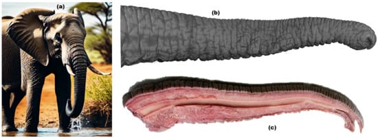
Figure 1.
(a) A photograph of an elephant with its trunk in a natural environment. (b) Dorsal view of the complete trunk specimen. (c) Left hemi-trunk before staining and scanning [1].
A novel approach to continuum robot backbone design, inspired by the flexibility and versatility of an elephant’s trunk, was introduced and validated in [2]. The proposed design incorporated helical compression springs with varying stiffness, arranged in a multi-section structure, allowing the robot to achieve smooth elongation, bending, and shortening. The paper focused on the effects of variable stiffness on its motion control and stability. Experimental results demonstrated that the variable stiffness backbone enhanced the robot’s rigidity, minimized twisting issues, and improved the efficiency of bending motions, particularly at the robot’s tip. This design offers potential improvements in control precision and adaptability in robotic applications requiring dexterous and compliant manipulation. However, the use of flexible springs increases the risk of buckling under excessive force along the backbone, which can compromise the robot’s stability and performance. Furthermore, while the design incorporates variable stiffness to improve control, this feature requires careful calibration and increases the complexity of the system.
A comprehensive mechanical model for a continuum robot, inspired by an elephant’s trunk, has been developed to predict the robot’s deformation under various conditions [3]. The robot’s modular structure incorporates adjustable stiffness across different segments, enabling adaptability to diverse tasks and environments. This adaptability is achieved through preprogrammable stiffness, which allows the robot to perform complex movements and adjust to varying curvature scenarios. Despite its versatility, the system’s complexity poses a significant challenge, as the precise control of stiffness across multiple segments demands intricate coordination between the hardware and software components.
The design and kinematic analysis of a bioinspired elephant trunk robot with a variable diameter showed that it offers significant advancements in the dexterity and adaptability of continuum robots [4]. The robot incorporates a soft motion mechanism combined with a rigid variable-diameter mechanism, enabling it to adjust its radial size and optimize performance for diverse tasks. This innovative design enhances the robot’s compliance, stiffness, and workspace versatility, allowing it to perform a wide range of motions with high precision. The kinematic model, which integrates both soft and rigid elements, was validated through simulations and experiments, demonstrating the robot’s capability to effectively adapt its shape and stiffness for complex manipulation tasks. Despite these advantages, the current design’s ability to change diameter is restricted to two discrete states, and the added weight of the mechanism may limit performance in certain applications. Future efforts will focus on developing a prototype with continuous diameter adjustment and minimizing the robot’s weight to further enhance its functionality.
In line with the advancements in bioinspired robotics, a variable-curvature elephant trunk robot (ETR) has been developed for applications in nuclear maintenance, particularly within the narrow and confined spaces of the China Fusion Engineering Test Reactor [5]. The ETR incorporates a miniaturized, lightweight design that balances flexibility and load-bearing capabilities, allowing it to perform precise inspection and maintenance tasks while maintaining high positional accuracy. Its kinematic model, developed using the Denavit–Hartenberg method, and trajectory-tracking control methods, including end-traction, discrete path, and base-fixed algorithms, were rigorously tested through simulations to validate its structural and motion performance. These control strategies enable the ETR to efficiently navigate complex trajectories, demonstrating the feasibility of deploying continuum robots in challenging environments such as vacuum chambers. This work highlights the potential for bioinspired designs to extend continuum robotics applications beyond traditional domains.
Building upon the inspiration derived from the physical intelligence of an elephant’s trunk, a recent study proposed a biomimetic soft robot with preprogrammable localized stiffness [6,7]. This innovative design employed interference plates to regulate localized stiffness without the need for additional devices, offering precise control over deformation and adaptability to complex scenarios. The study demonstrated the capability to efficiently adjust stiffness by preprogramming stiffness profiles, significantly reducing the reconstruction time and enhancing environmental compliance.
However, challenges remain, particularly concerning the construction of the continuum model. The research work discussed above primarily focused on the flexible components of continuum robots, such as trunk-like structures, while largely excluding considerations of the rigid parts, such as the wrist or prearm, that are often critical for certain applications. The development of such models requires intricate design considerations, including balancing flexibility and structural integrity, accurately modeling the dynamic behavior of the system, and addressing the complexity of implementing effective trajectory-tracking algorithms. Additionally, a miniaturized and lightweight design, while advantageous for confined spaces, can result in limitations such as a reduced load capacity and increased susceptibility to external forces, which may compromise stability and precision during operation. These drawbacks highlight the need for further research to integrate rigid and flexible components into a unified framework, optimizing the construction and control strategies of continuum models for demanding applications.
To address these complexities, the multibody system approach provides a robust framework for modeling the dynamics of systems comprising rigid and flexible components [8]. By integrating continuum mechanics within the multibody dynamics framework, formulations such as the Absolute Nodal Coordinates Formulation (ANCF) enable the precise modeling of large deformations and large rotation problems [9,10]. Unlike simplified assumptions of constant curvature or discrete elastic rod models, the ANCF allows for the comprehensive representation of structural flexibility, geometric nonlinearities, and cross-sectional distortions. This approach not only enhances the accuracy of dynamic simulations but also supports the development of integrated kinematic and static models, enabling sophisticated applications in soft and continuum robotics.
However, modeling the rigid–flexible interface in multibody systems presents significant challenges due to the contrasting dynamic characteristics of rigid and flexible bodies. Rigid bodies require simplified modeling, often focusing on positional and orientational coordinates, while flexible bodies necessitate a detailed representation of deformations, strain distributions, and dynamic interactions. This disparity introduces complexity in coupling these components within a unified framework.
The strain-based nonlinear beam formulation, as presented in [11], provides an effective approach for analyzing complex rigid–flexible interfaces. It enhances computational efficiency and stability by employing strain measures and minimizing cross-sectional deformations, making it particularly suitable for slender, geometrically nonlinear systems. While it reduces the number of variables and achieves better convergence compared to the ANCF, its integration into multibody frameworks requires substantial modifications, and its applicability to complex or non-slender geometries remains unclear.
The Natural Coordinates Formulation (NCF) [12,13,14] offers an effective method for modeling rigid bodies using Cartesian coordinates that inherently increase the number of shared coordinates among interconnected rigid–flexible bodies. This formulation is particularly effective in systems with Differential Algebraic Equations (DAEs), as it ensures the mass matrix remains constant and simplifies the integration of linear constraints.
Despite these advantages, the NCF faces challenges such as high computational demands, issues with constraint stabilization, locking problems, and difficulties in modeling complex cross-sectional structures. This work aimed to address these challenges to meet the intricate requirements of rigid–flexible interfaces in modeling an elephant’s trunk, serving as a framework for continuum manipulators where both accuracy and computational efficiency are essential.
This document is structured as follows: Section 2 explores the anatomy of an elephant’s trunk. Section 3 delineates the Natural Coordinates Formulation (NCF), focusing on its application in rigid body dynamics, the implementation of rigidity constraints, and the derivation of the mass matrix and generalized forces. Section 4 delineates the Absolute Nodal Coordinates Formulation (ANCF), including the kinematics of the ANCF thin plate element, the derivation of generalized forces, and validation studies utilizing dynamic models of initially straight or curved configurations. Section 5 outlines the ANCF continuum trunk model, incorporating the geometric modeling and finite element representation of the elephant trunk. Section 6 explains the rigid–flexible coupling dynamics between the elephant’s head and trunk. Section 7 addresses dynamic simulations, highlighting the use of stabilization methods and numerical integration techniques. The conclusion is detailed in Section 8.
2. Elephant’s Trunk Anatomy
Figure 1 provides a comprehensive view of an elephant’s trunk, starting with a photograph taken in its natural environment that showcases its flexible, muscular structure and characteristic wrinkled skin. A 3D reconstruction (Panel b) emphasizes the trunk’s intricate surface details and cylindrical shape, highlighting the complexity of its external musculature. Finally, a cross-sectional view (Panel c) reveals the internal anatomy, detailing the arrangement of muscles and tissues that enables the trunk’s function as a muscular hydrostat. Together, these images illustrate the trunk’s dense musculature, consisting of approximately 90,000 muscle fascicles, which grants it extraordinary dexterity and fine motor control.
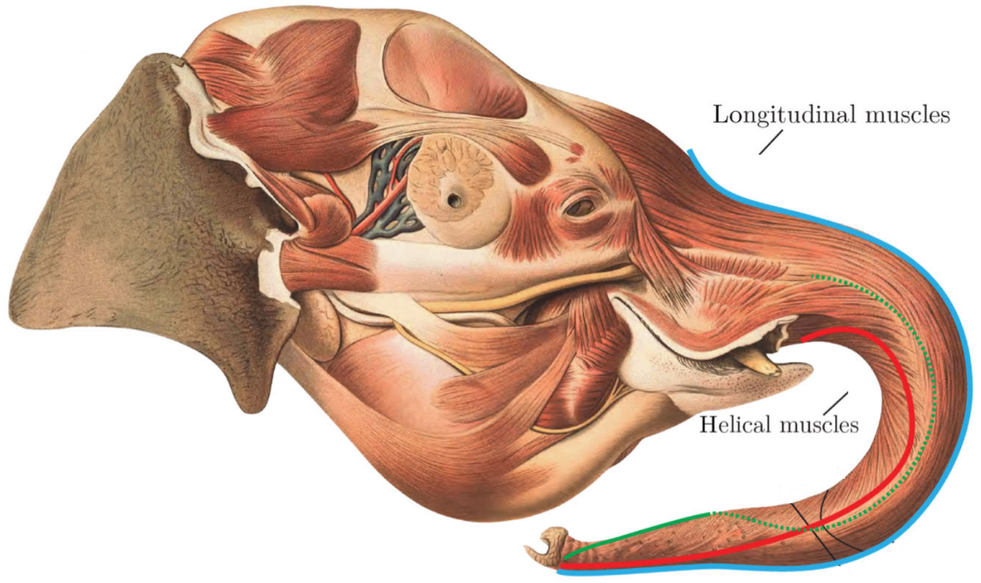
An elephant’s trunk exhibits a remarkable range of motion configurations, allowing it to perform various complex tasks such as drinking, feeding, and grasping objects. This versatility is achieved through the coordination of 17 distinct muscle groups that control the trunk’s movements. Key configurations include bending, where longitudinal muscles contract on one side to curl the trunk into various shapes, and torsion, enabled by helical muscle fibers that allow the trunk to twist in multiple directions; see Figure 2. The trunk can also perform combined motions, seamlessly integrating bending and twisting to enhance its ability to interact with its environment. These configurations collectively contribute to the trunk’s extensive reach and flexibility, enabling it to access a broad volume of space, often referred to as the “reachability cloud”, making the trunk an incredibly adaptable and efficient appendage for a wide range of tasks [15].

Figure 2.
Elephant trunk with longitudinal muscles [15].
Due to the dominant influence of the skull’s rigid structure on the overall motion of the elephant’s head, soft tissue effects are considered negligible in the context of the rigid–flexible coupling approach. Therefore, the head is modeled as a rigid body using the Natural Coordinates Formulation (NCF), while the trunk is treated as a flexible body using the Absolute Nodal Coordinates Formulation (ANCF), providing an integrated framework to accurately capture the dynamics and motion of this complex system.
3. Natural Coordinates Formulation (NCF)
The NCF is specifically designed for analyzing systems that consist of both rigid and flexible bodies. When used on rigid bodies, the NCF offers an alternative to conventional approaches that employ reference frames and generalized coordinates to describe the kinematics and dynamics of a system. The NCF directly employs the absolute positions of select points, along with the orientations of vectors that are fixed in the body, as the primary coordinates. This choice simplifies the representation of constraints and the equations of motion, leading to models that are often more intuitive and straightforward to implement for certain types of problems.
3.1. Modeling Rigid Body Dynamics with NCF
The first step involves selecting specific points and vectors on the rigid body that uniquely define its position and orientation in space. For instance, two points could determine a line segment representing a rigid link’s orientation and length, while an additional non-collinear point could establish the body’s plane.
An elephant head, which is rigidly connected to the trunk, is regarded as a rigid body that can be described and formulated via the Natural Coordinate Formulation (NCF). The NCF is a method used in the kinematic and dynamic analysis of rigid multibody systems; a special feature of the NCF is that it leads to the generation of a constant mass matrix, which simplifies the computational process, and the generalized inertia forces, such as centrifugal and Coriolis forces, are zero, which is advantageous for analysis [16].
The rigid body is described in the Natural Coordinates Formulation (NCF) by the Cartesian coordinates of the basic points distributed throughout the body and by the Cartesian components of several unit vectors attached to these points that describe the orientation of the rigid body. For a spatial rigid body which is described with two points and two non-coplanar unit vectors, shown in Figure 3, the vector of the generalized coordinates of a rigid body can be expressed as
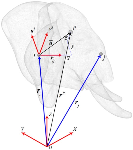
Figure 3.
Kinematics of rigid body using Natural Coordinate Formulation.
For a rigid body with a rectangular cross-section with a length of l, width of w, and height of h, one can conclude that
3.2. Rigidity Constraints
The description of a rigid body with two basic points and two non-coplanar unit vectors leads to twelve natural coordinates and six degrees of freedom; six constraint equations must be imposed. These six conditions are one constant distance equation, two unit module conditions for the unit vectors, and three constant angle conditions between the two vectors and the segment and between the two vectors themselves.
3.3. Obtaining the Mass Matrix of the Rigid Body Using the NCF
The mass matrix for rigid bodies can be obtained by integrating the density-weighted mass contributions throughout the body’s volume using the Natural Coordinates Formulation (NCF), in which the position of points directly defines the rigid body configuration. The mass matrix is computed as follows:
Explicity, the mass matrix can be written as
It is important to note that the NCF-based mass matrix depends on the mass distribution and the selected coordinates. Unlike other formulations for modeling rigid body motion, no rotational parameters or time-dependent transformations are used. As shown in Equation (9), the use of the NCF results in a constant mass matrix derived from the shape function matrix of the body [17].
3.4. Derivation of Generalized Forces of Rigid Body Using NCF
In the context of the Natural Coordinates Formulation (NCF), deriving the generalized forces due to the applied forces is well established in the literature. However, the derivation of the generalized forces due to the applied moments presents greater complexity due to the absence of rotational angular coordinates in the NCF. Consequently, we begin with the derivation of the generalized forces due to moments. For the applied moments, the virtual work principle can be expressed as
When combining the effects of both forces and moments, the complete vector of the generalized forces takes the form
The equation of motion is obtained by using the method of Lagrange multipliers as
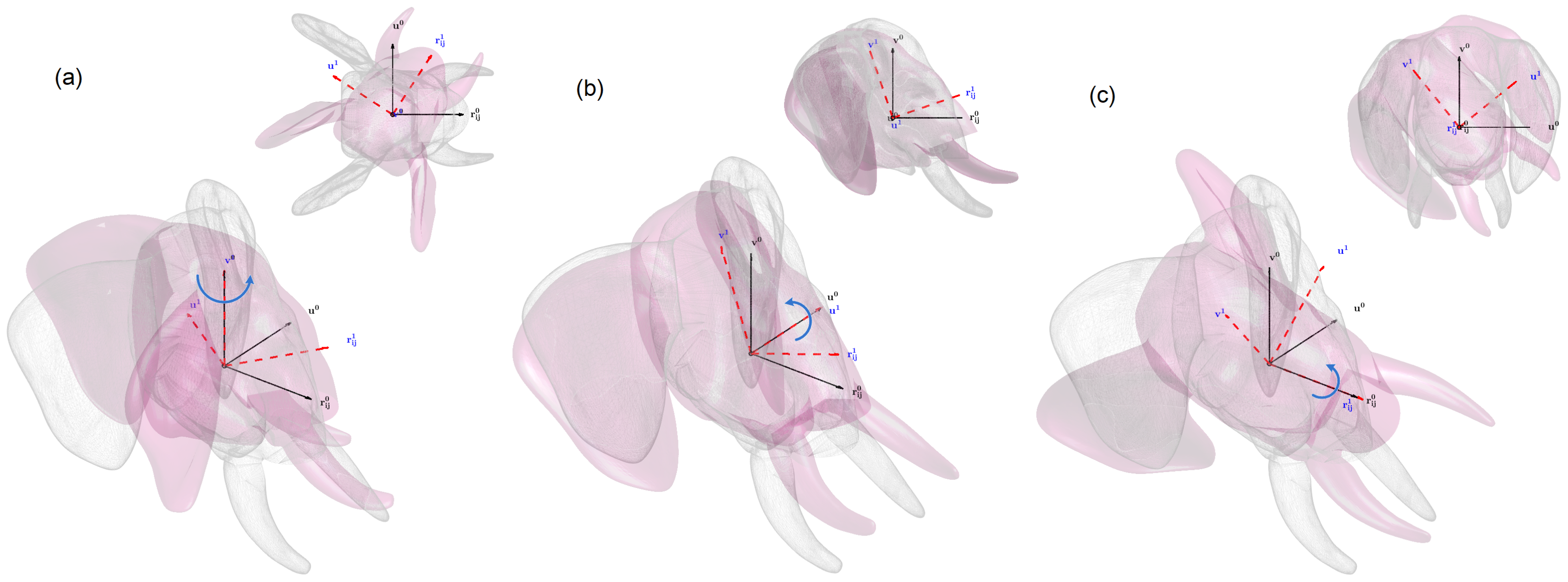
Figure 4 illustrates the effect of applying moments along different axes of an elephant’s head, modeled as a rigid body. In this example, the head is spherically attached to a fixed constraint, allowing for rotation while maintaining a fixed position. The rigidity constraints, as described in Equation (7), ensure that the body’s motion adheres to its structural limitations. The application of moments about the z-axis, y-axis, and x-axis, shown in subfigures (a), (b), and (c), respectively, demonstrates the resultant rotational effects.
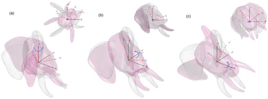
Figure 4.
Motion of rigid body due to moments applied to rigid body: (a) about z-axis, (b) about y-axis, (c) about x-axis.
4. Absolute Nodal Coordinates Formulation
The Absolute Nodal Coordinates Formulation (ANCF) is widely used for the dynamic analysis of multibody systems. It is particularly well suited for modeling continuum elements subjected to large rotations and large deformations, making it ideal for applications that require capturing the highly flexible and nonlinear behavior of structures [18,19,20]. Many applications are modeled using ANCF elements, including wind turbine blades, piezoelectric composites, tire models, belt drives, aerospace systems [21,22,23], and others. In this context, the ANCF provides a robust framework to model the overall dynamics of an elephant’s trunk, including its interactions with the environment and the effects of gravitational and other external forces. The formulation’s ability to accurately represent deformation and motion makes it a powerful tool for analyzing complex, flexible systems like an elephant’s trunk.
4.1. Kinematics of ANCF Thin Plate Element
Over the years, several ANCF elements have been introduced, evolving from 2D to 3D formulations, including beams, plates, shells, and cables, further expanding the versatility of the ANCF approach [24,25,26]. In the ANCF, position and gradient vectors are used as nodal coordinates; this formulation leads to a constant mass matrix and, as a consequence, the centrifugal and Coriolis inertia forces are identically equal to zero, which has a great advantage for dynamic analysis. In this paper, the ANCF thin plate element is employed for modeling the continuum model of an elephant trunk.
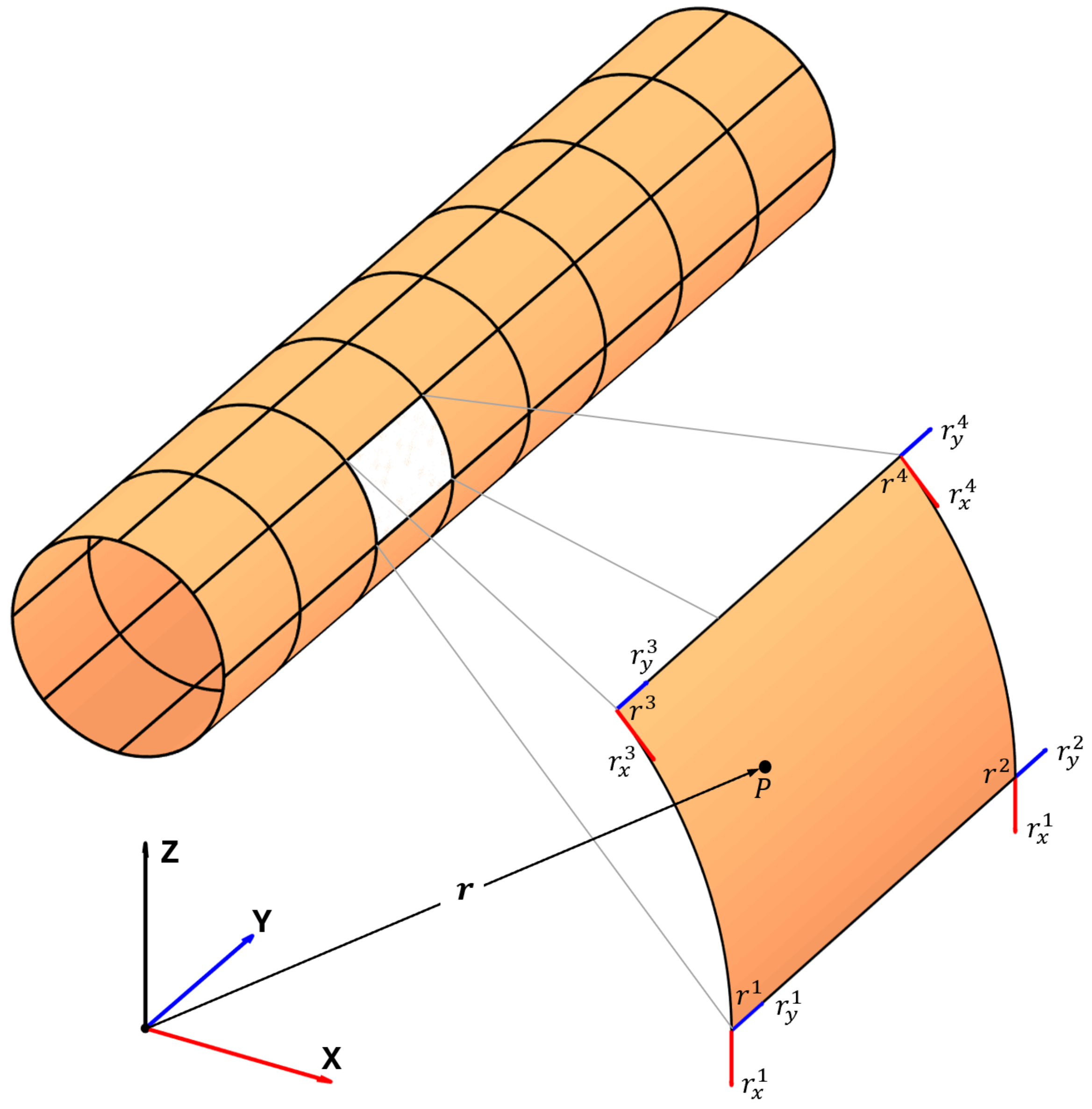
The ANCF thin plate element assumes that the plate has a constant thickness and does not consider the deformation along the thickness direction. The four corner points of the mid-surface are used as element nodes, with each node having a position vector and two gradient vectors as nodal coordinates with nine degrees of freedom, leading to a reduced-order element with 36 degrees of freedom [27]. The global position vector of an arbitrary point, P, on the mid-surface of the thin plate element can be defined as
where is the element shape function matrix, and is the vector of the nodal coordinates. This vector at node i of an element can be defined as
The nodal coordinates of one element can be expressed by the vector , which includes the nodal coordinates of the four nodes, as
where is the global position vector, and define the gradient vectors at the node i, and the element shape function matrix for a thin plate element can be obtained using incomplete third-order polynomial interpolation functions where the basis can be obtained from Pascal’s triangle [28].
The shape function matrix can be expressed as
where is a third-order identity matrix and shape functions can be defined as
where and are the local normalized coordinates and a and b are the length and width of the finite element in the reference configuration.
Based on the general continuum mechanics theory, three configurations can be involved in describing the deformation of the ANCF element. Figure 5 illustrates the straight configuration , the initial reference configuration (stress-free) , and the current deformed configuration . Integration and differentiation are applied to the straight configuration using the matrix of the position vector gradient , where and is the vector of the element nodal coordinates in the initial reference configuration. Another matrix of the position vector gradient is utilized to establish the relationship between the current and straight configurations [29], thus
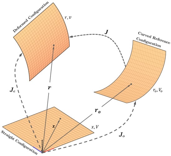
Figure 5.
Various related configurations for ANCF plate.
In the fully parameterized elements, the position vector gradient is a matrix. However, the gradient-deficient element has only two gradient vectors as the deformation along the thickness direction is not considered, and as a consequence, the matrix of the position vector gradients is not square. In order to allow for using the standard procedure as in the general continuum mechanics approach, the unit normal vector at the mid-surface, which is not a position vector gradient, is inserted to ensure that the gradient of the position vector forms a square matrix [20,30].
The volume in the current deformed configuration v and the volume of the curved reference configuration are related to the volume of the straight configuration V through the relationship and , where is the determinant of the position gradient matrix for the initial configuration, which means that integration over the domain can be transformed to the straight element domain V.
The zero strain of the initially curved reference configuration can be obtained by using the inverse of the matrix of the position vector gradients evaluated for the curved reference configuration as and .
The generalized inertia forces can be obtained by evaluating the kinetic energy T of the element as
4.2. Generalized Forces of Thin Plate Element
The generalized nonlinear elastic forces vector is obtained in the current configuration concerning the stress-free reference configuration, which may have a curved geometry. The strain energy of the thin plate element is obtained based on the membrane effect and the curvature of the mid-surface:
The elastic forces can be obtained by differentiating the strain energy by the vector of the element nodal coordinates:
4.3. Validation of Elastic Forces Model of Thin Plate Pendulum
The dynamic problem of a free-falling thin plate pendulum provides a robust benchmark to assess the accuracy and computational efficiency of finite element models under large deformation and rotational dynamics [27].
In this study, the pendulum plate depicted in Figure 6 was modeled using ANCF thin plate elements with an edge length of 0.3 m and a thickness of 0.01 m. The material properties included a mass density of 7810 kg/m3, a Young’s modulus of , and a Poisson’s ratio of 0.3. Initially, the plate was in a straight configuration, with one corner constrained and connected to the ground via a spherical joint. Upon release, the plate fell under the influence of gravitational acceleration (), showcasing its dynamic behavior and deformation over time.
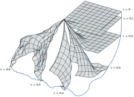
Figure 6.
Dynamic analysis of the straight pendulum.
The governing equation of motion for this problem, expressed in terms of the constant mass matrix , nonlinear elastic forces , and external forces , is given as
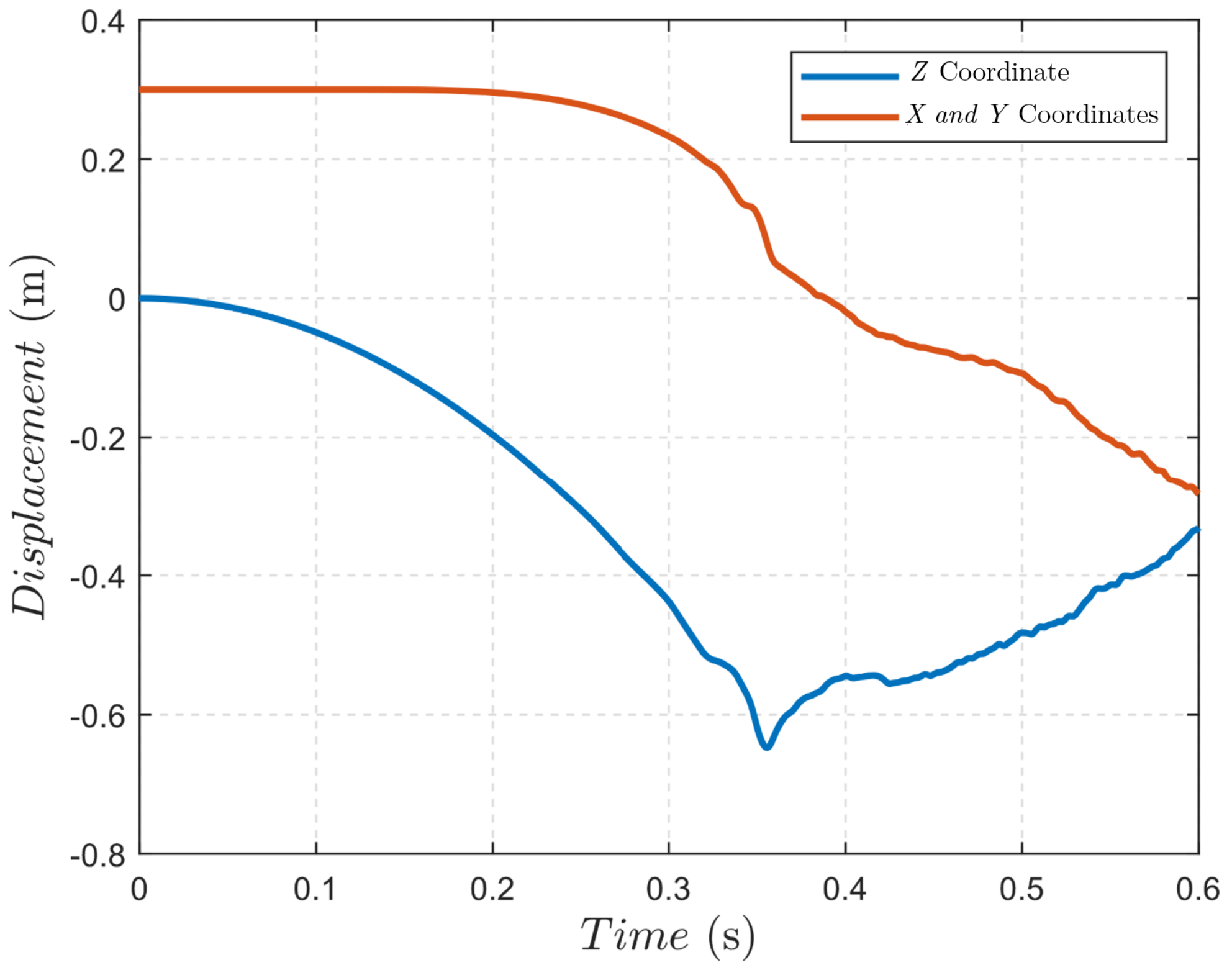
Figure 6 illustrates the dynamic response of the thin plate pendulum at various time instances (), highlighting the progressive deformation of the plate as it fell. The evolution of the displacement of the pendulum’s corner point is shown in Figure 7, where the coordinates over time reveal the nonlinear trajectory and significant deformation experienced by the plate.
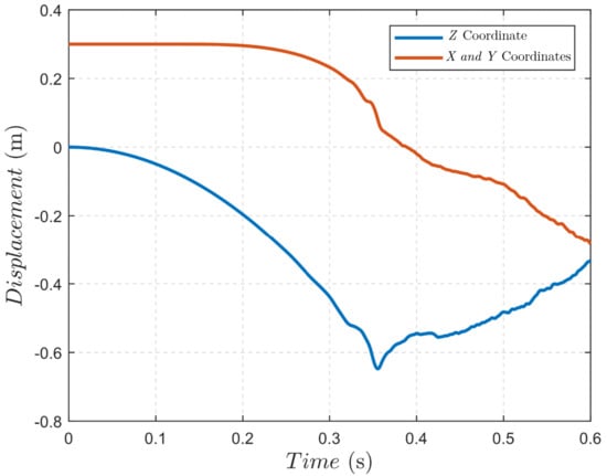
Figure 7.
Position of the corner point.
To ensure the validity of the simulation, an energy conservation analysis was performed, as shown in Figure 8. This figure presents the energy balance at each time step, including for the potential energy (U), strain energy (W), kinetic energy (T), and total energy. The consistent total energy across all time steps demonstrates that the ANCF plate element adheres to the work and energy principles, providing a reliable representation of the dynamic behavior of the system.
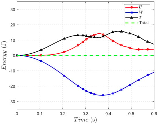
Figure 8.
Energy conservation of the pendulum.
4.4. Validation of Elastic Forces of Initially Curved Pendulum
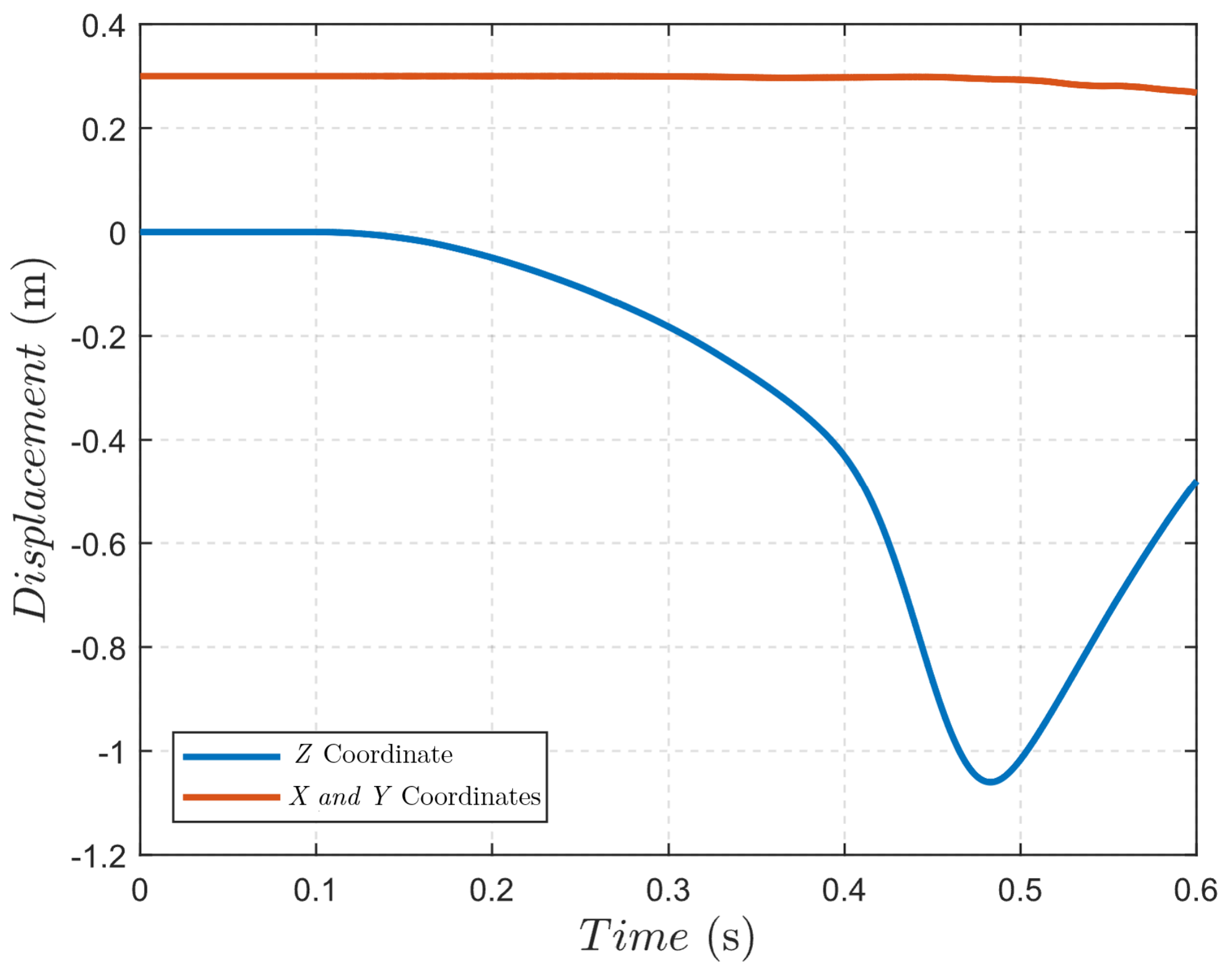
The initially curved pendulum fell under the effect of the gravity as illustrated in Figure 9; it was modeled using ANCF thin plate elements. The dimensions and material properties were the same as for the straight pendulum, except a Young’s modulus of was used. The application of the external force started at 0.1 s of the simulation time to show the zero strain of the initially curved configuration. Figure 10 shows the coordinates over time. It can be observed from Figure 11 that the strain energy remained at zero within the first 0.1 s of the simulation, because there were no external forces applied during that time interval. Also, the sum of the strain, kinetic, and potential energies remained constant during the simulation.
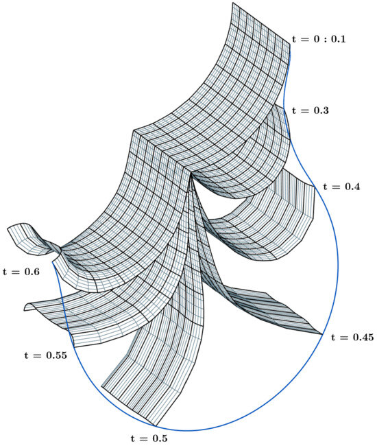
Figure 9.
Motion analysis of the initially curved pendulum.
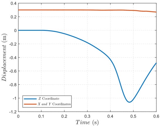
Figure 10.
Position of the corner point.
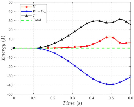
Figure 11.
Energy of the curved pendulum.
The results confirm that the ANCF thin plate element not only captures the complex deformations of the plate with high accuracy but also achieves computational efficiency by using a minimal number of elements. This capability makes the ANCF framework a powerful tool for analyzing flexible multibody systems subjected to large deformations and external forces.
5. ANCF Continuum Trunk Model
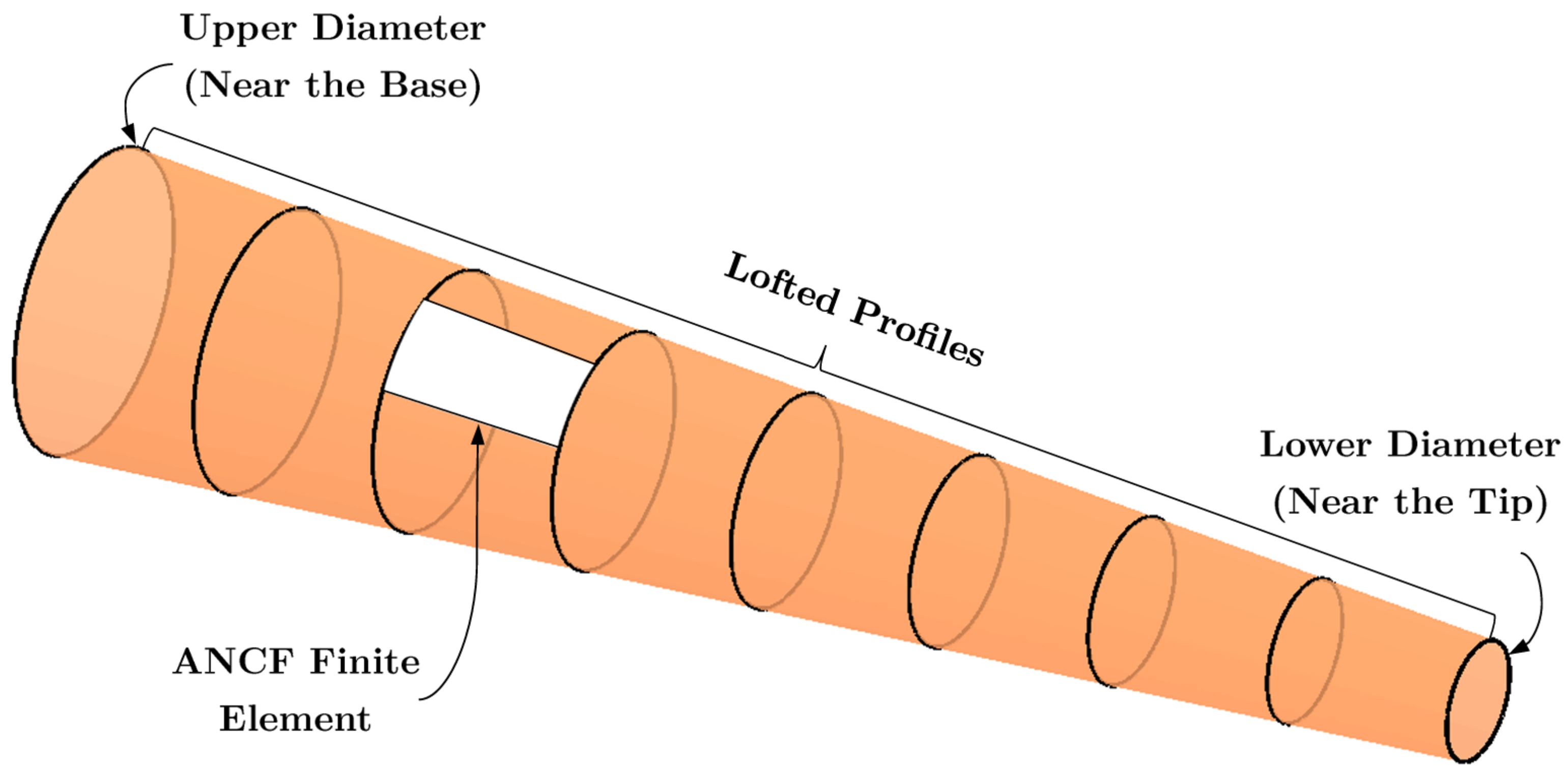
ANCF gradient-deficient plate finite elements were used to model the geometry and conduct the analysis of the trunk. A dedicated subroutine was developed in MATLAB to automate the construction of the trunk’s tubular structure. The subroutine systematically defined the elements in a clockwise direction for each cross-sectional slice, progressing sequentially along the elastic centerline of the trunk. The generation of the nodal points is shown in Figure 12. The generated nodal coordinates were then used to assemble the ANCF finite elements, enabling the simulation of the complex deformations and movements of the trunk.
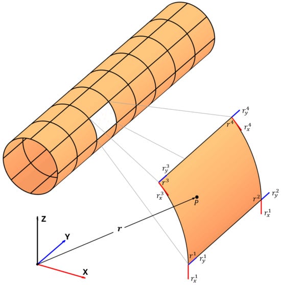
Figure 12.
Generation of tubular structure using ANCF thin plate element.
The lofted profiles were obtained by transforming the position coordinates of the upper cross-sectional mesh points, see Figure 13, which can be expressed as

Figure 13.
Tubular trunk ANCF model generated using thin plate element.
- is the homogeneous scaling matrix, defined as
- is the radius at position k, given by
- is the homogeneous translation matrix, defined as
Here, is the lower radius, and L is the length of the trunk.
Continuum Trunk Model Analysis: The dimensions and material properties of the continuum trunk model were based on empirical data from a mature female Asian elephant at the National Zoo in Washington, D.C. [31]. The trunk was m long with an upper diameter of 32 cm near the head, tapering to a lower diameter of 8 cm towards the tip. This gradual tapering provided an anatomically accurate representation of an elephant’s trunk. The material properties for the model included a density of 1180 kg/, a Young’s modulus of N/, and a Poisson’s ratio of . Initially positioned in a horizontal configuration, the trunk was allowed to fall naturally under the action of gravity, simulating real-world behavior over a duration of seconds. Figure 14 illustrates this motion, highlighting the trunk’s deformation as it transitioned into a downward curve due to gravitational forces.
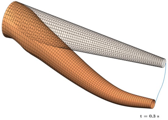
Figure 14.
Wireframe illustration of falling trunk structure under gravity.
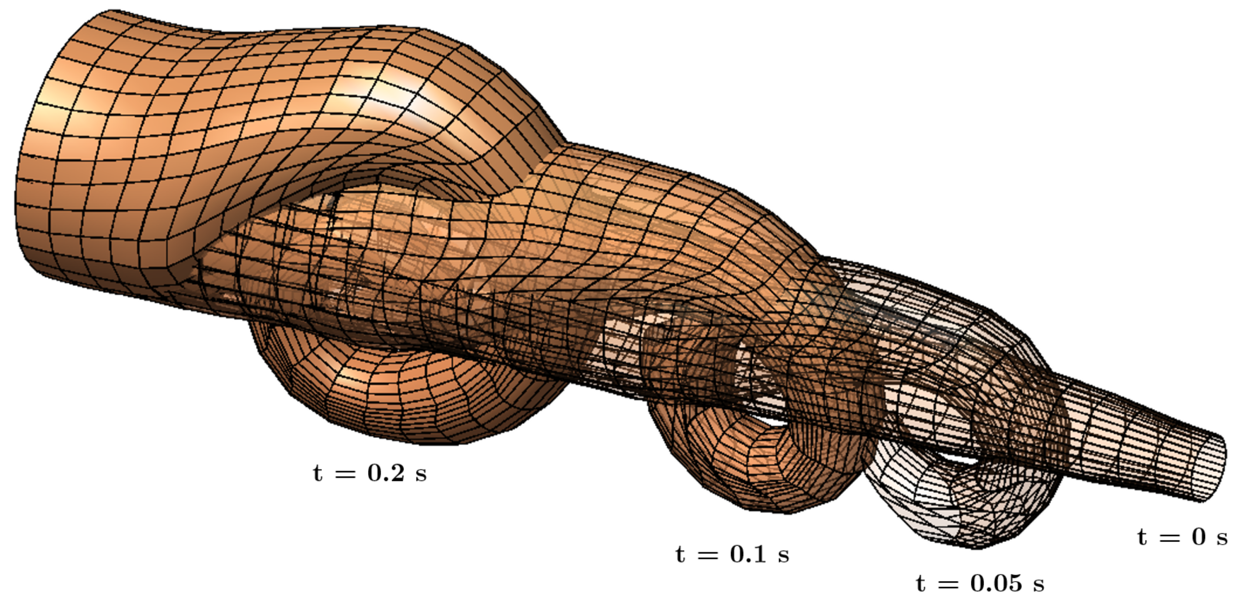
In addition to gravitational loading, external bending moments were applied along the length of the trunk to simulate coiling or bending actions, as shown in Figure 15 and Figure 16. This captured one of the trunk’s most vital functions: its ability to bend or coil during activities such as grasping or wrapping around objects. To achieve this, a direct methodology was employed to impose concentrated moments on the ANCF finite elements, leveraging the framework proposed in [10,13].
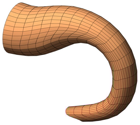
Figure 15.
Wireframe illustration of bending the continuum trunk structure.

Figure 16.
Wireframe illustration of a dynamic analysis of the trunk coiling.
These simulations demonstrated the model’s ability to realistically replicate the complex mechanics of an elephant’s trunk, including large deformations and the intricate interplay between the gravitational forces and applied moments. This validated the effectiveness of the ANCF in modeling biological structures with high degrees of flexibility and adaptability.
It can be concluded that the third-order polynomial interpolation function given in Equation (23), which was employed for thin plate elements, achieved an acceptable balance between computational efficiency and accuracy. While higher-order interpolation functions could enhance precision, they significantly increase computational complexity, memory requirements, and the processing time. Figure 15 and Figure 16 show that the third-order formulation effectively captured the trunk’s deformation while maintaining numerical stability and efficiency, making it well suited for dynamic simulations.
6. Rigid–Flexible Coupling
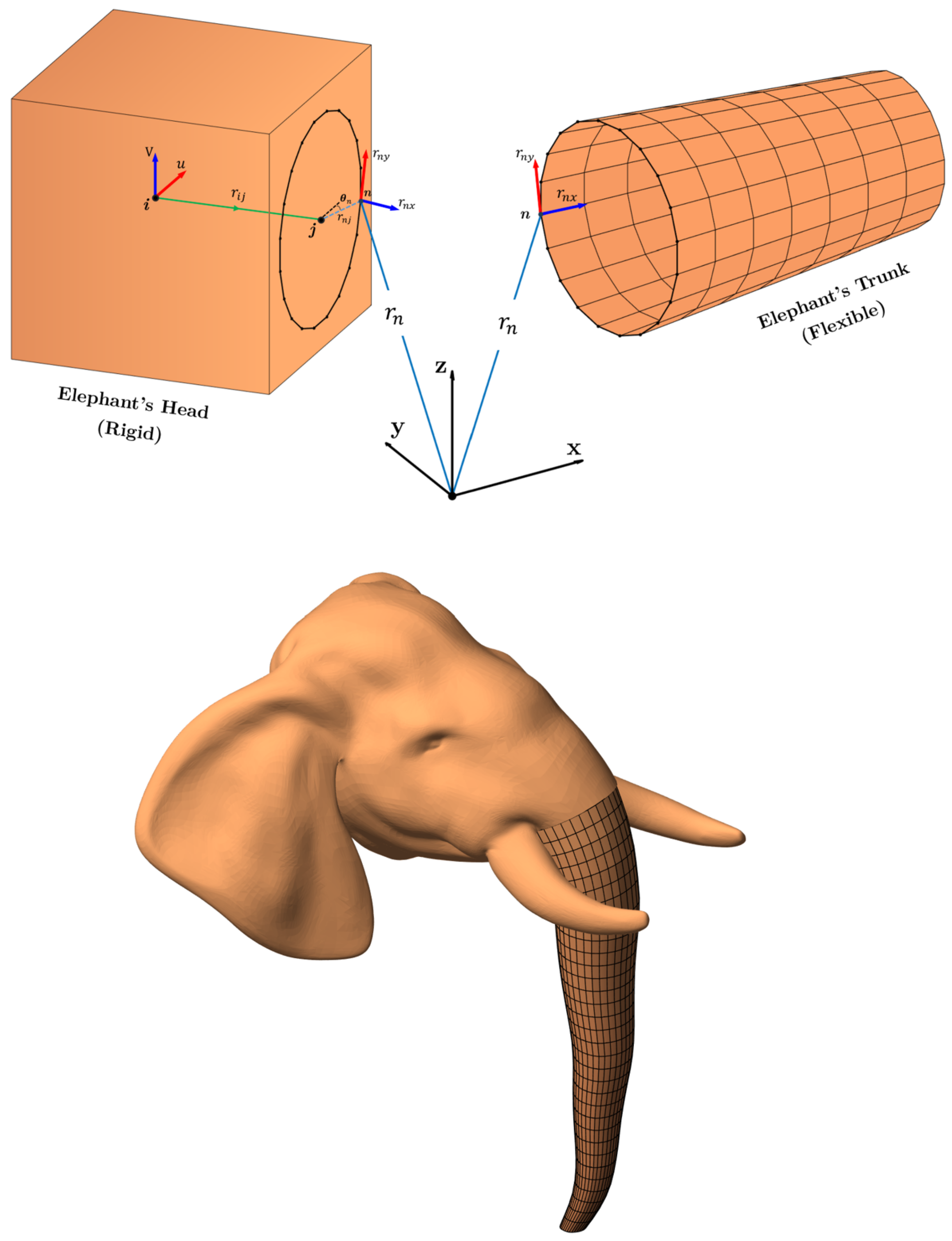
The interaction between an elephant’s head and trunk as a multibody biomechanical system was described based on the hybrid Natural and Absolute Nodal Coordinates Formulation (NCF/ANCF) framework for rigid–flexible coupling. The head in this context was modeled using the Natural Coordinate Formulation (NCF), which accurately captured the rigid nature of the head structure, while the trunk was developed and described using the Absolute Nodal Coordinate Formulation (ANCF), which is appropriate for large deformation and rotation analysis in flexible multibody systems.
Figure 17 shows the interaction between the elephant’s trunk and the head it is rigidly attached to. The connection layer consists of mesh points that determine the rigid clamped joint which constrains the relative translation and rotation between the rigid and flexible bodies. The position vector and gradient vectors and at node n of the flexible body are fully constrained by the point , , and vectors of the rigid body.

Figure 17.
Constraint formulation of rigid–flexible coupling and resulting head–trunk model.
The constraints equation of the clamped joint between the flexible body (trunk) and the rigid body (head) can be defined as
The constraint function imposes a certain distance, , between point on the rigid body and nodes from to , which correspond to meshed nodes along the cross-section of the flexible body in contact with the rigid body. This ensures that the relative distance between these two points remains constant so that the geometric or kinematic relationship is maintained; these constraints can be defined as
The constraint function ensures that the angle between the vectors and remains constant, even as the bodies move within the system. This constraint ensures that the relative orientation between the two vectors or bodies is maintained; these constraints can be defined as
The angle between the vectors and can be calculated as
The orthogonality constraint ensures that two vectors remain normal to each other, which can be defined as
The overall constraint equations, including the rigidity constraints of the rigid body described in the NCF and the rigid–flexible coupling constraints, can be represented as
Notably, the rigid head assumption is enforced through a set of constraint equations, Equations (44)–(47) within the NCF framework, which can be selectively relaxed to introduce some degree of soft tissue elasticity, if needed.
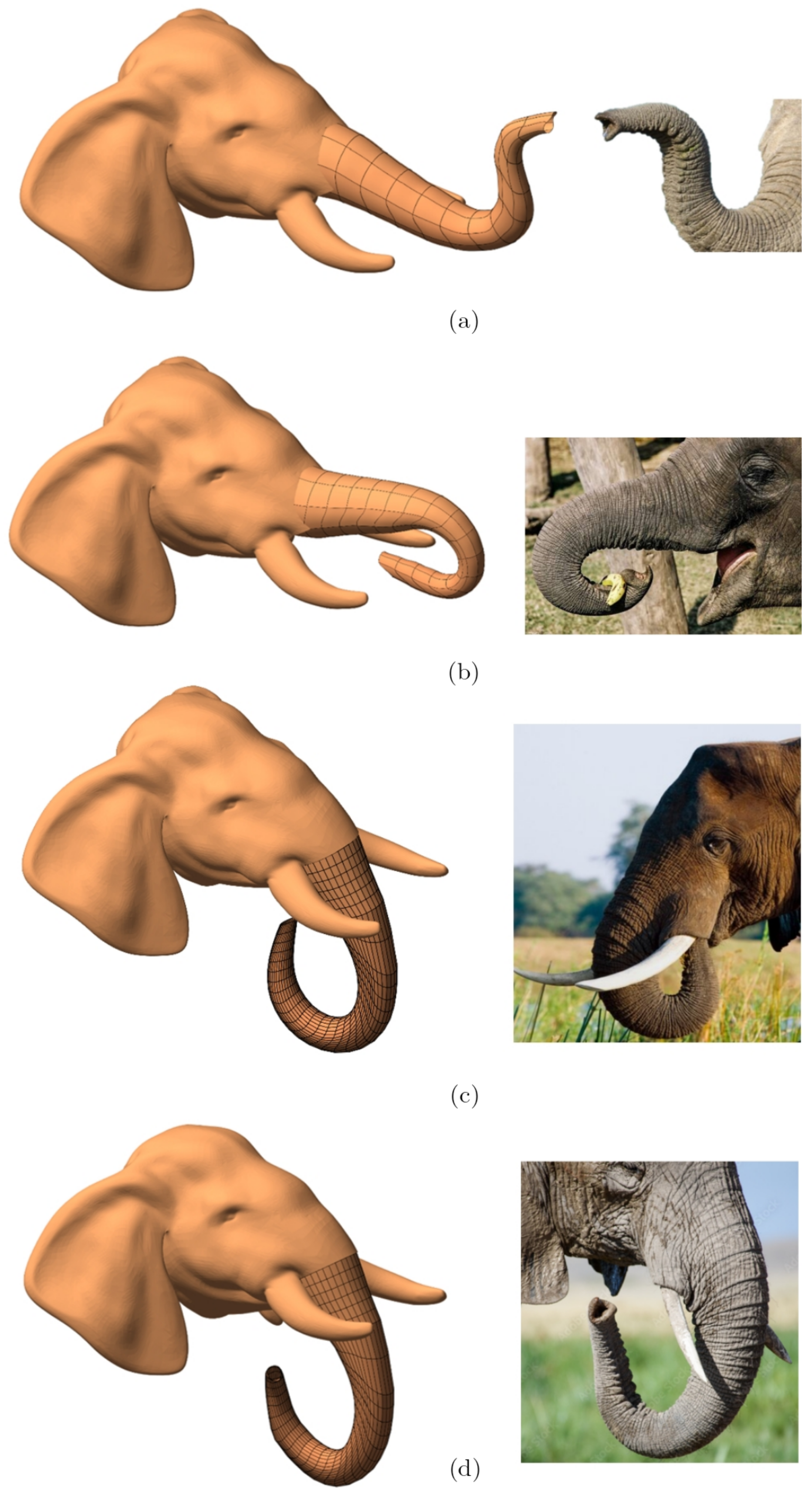
The kinematic movements of the elephant’s trunk, as illustrated in Figure 18, highlight the model flexibility and precision of the proposed rigid–flexible interface and its interaction with the environment. These motions include bending, twisting, and their combinations, each demonstrating the intricate coordination and strength of the trunk’s musculature. The trunk’s ability to extend outward with partial flexion allows it to delicately manipulate objects, showcasing its precision and fine motor control. In such scenarios, a slight upward curve at the tip suggests the careful adjustments required for grasping or repositioning items with accuracy.

Figure 18.
Kinematic movements of an elephant’s trunk: (a) Manipulating (Extension and Partial Flexion): The trunk extends outward to reach and interact with the object; the slight upward flexion at the tip suggests the delicate precision required for picking up or manipulating items. (b) Picking (Coiled Flexion with Gripping): The trunk is tightly coiled around an object, which requires the precise activation of transverse and oblique muscles, enabling the trunk to obtain a secure grip on the object. (c) Eating Directly (High Flexion with Lifting): The trunk lifts the food item directly to the mouth without additional manipulation. Flexion and upward lift are characteristic of this motion, achieved through transverse and dorsal muscle activation. (d) Gripping (High Coiled Flexion): The trunk grips the object, coiling to apply precise force for some actions. This involves a combination of transverse and oblique muscle activation.
7. Dynamic Simulation
In order to carry out the dynamic simulation of the elephant’s head–trunk system, the equations of motion, as presented in Equation (17), were modified for the rigid–flexible multibody system, taking the form of
Examples of the dynamic simulations are presented in Figure 19 and Figure 20. The first example shows the efficiency of the interaction of the two bodies, by applying constant torque to the rigid body while no load or gravity was acting on the flexible body. An additional example of the interaction between the two bodies is that the flexible body was subjected to a bending moment, while there were no external or gravitational forces acting on the rigid body.

Figure 19.
Dynamic simulation of an elephant’s head–trunk system when torque is applied to the rigid head.
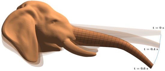
Figure 20.
Dynamic simulation of an elephant’s head–trunk when the trunk is subjected to a bending moment.
These simulations highlight the complex interaction of external forces and internal constraints essential for realistic system movements. To accurately capture this complexity, the equations of motion were formulated as a system of Differential Algebraic Equations (DAEs), incorporating holonomic constraints that govern the system’s geometry and motion.
A Baumgarte stabilization approach [32] was employed to mitigate constraint violations at the position and velocity levels during numerical integration. Equation (51) is a second-order differential equation determining the kinematic constraints; the two terms and in this equation perform the role of PD control. The numerical values of and were empirically chosen as stabilization parameters (damping ratio of ⇔ and ) [33]. While this approach shows effective results for rigid-body systems and for short simulations, this method often fails in flexible multibody systems to prevent the “drift effect”, especially in long simulations, due to the fixed numerical values of its parameters throughout the simulation.
To enhance stability and accuracy, the Fuzzy Logic Control (FLC) constraint stabilization method was implemented [34]. This method introduces a control framework independent of the system dynamics, effectively suppressing constraint violations over long simulations. The FLC framework utilizes Sugeno-type systems with Gaussian membership functions to provide robust stabilization, making it particularly suitable for the hybrid head–trunk model.
The implemented FLC operates through three primary phases of fuzzification, fuzzy rule-based decision making, and defuzzification. During the fuzzification phase, the inputs are the constraint function and its derivative , which are normalized using scaling factors ( and ) to ensure the fuzzy input variables are within the range of and transferred into fuzzy sets using membership functions. Based on a comparison between several fuzzy sets, including triangular, trapezoidal and Gaussian memberships, the results indicated that Gaussian membership functions offer greater stability of the numerical solution, reduce constraint violations, and enhance computational efficiency. The rule-based decision making phase acts upon the fuzzy inputs with a set of rules to make appropriate corrective actions. Defuzzification converts the fuzzy outputs into crisp values for the purpose of stabilization corrections. The FLC output is estimated by a Sugeno-type system, significantly enhancing the efficiency of defuzzification. Unlike the Mamdani approach, whose distributed fuzzy sets require computationally expensive calculations, the Sugeno approach utilizes a singleton output membership function, a single spike representation [34].
Violations in the constraints in the system create unknown disturbances, represented as . These disturbances affect the motion of the system, and thus
In order to compensate for this drift, the FLC generates the adjusting action, , ensuring that the system remains stable. FLC compensates for drifting by setting , leading to the modified equation
This equation can be simplified to
When applying the FLC approach for stabilization, the system dynamically adjusts to minimize constraint violations and maintain accurate motion. This technique enhances stability, and thus it is suitable for complex multibody simulations.
The numerical solution employs a variable-step, variable-order integrator, namely, the Adams–Bashforth–Moulton method, which is a multistep predictor–corrector integration approach. When paired with the FLC stabilization strategy, the computational efficiency and stability are optimized. It can be concluded that this approach ensures precise constraint handling and dynamic consistency, even under complex loading scenarios, such as lifting, bending, and twisting movements.
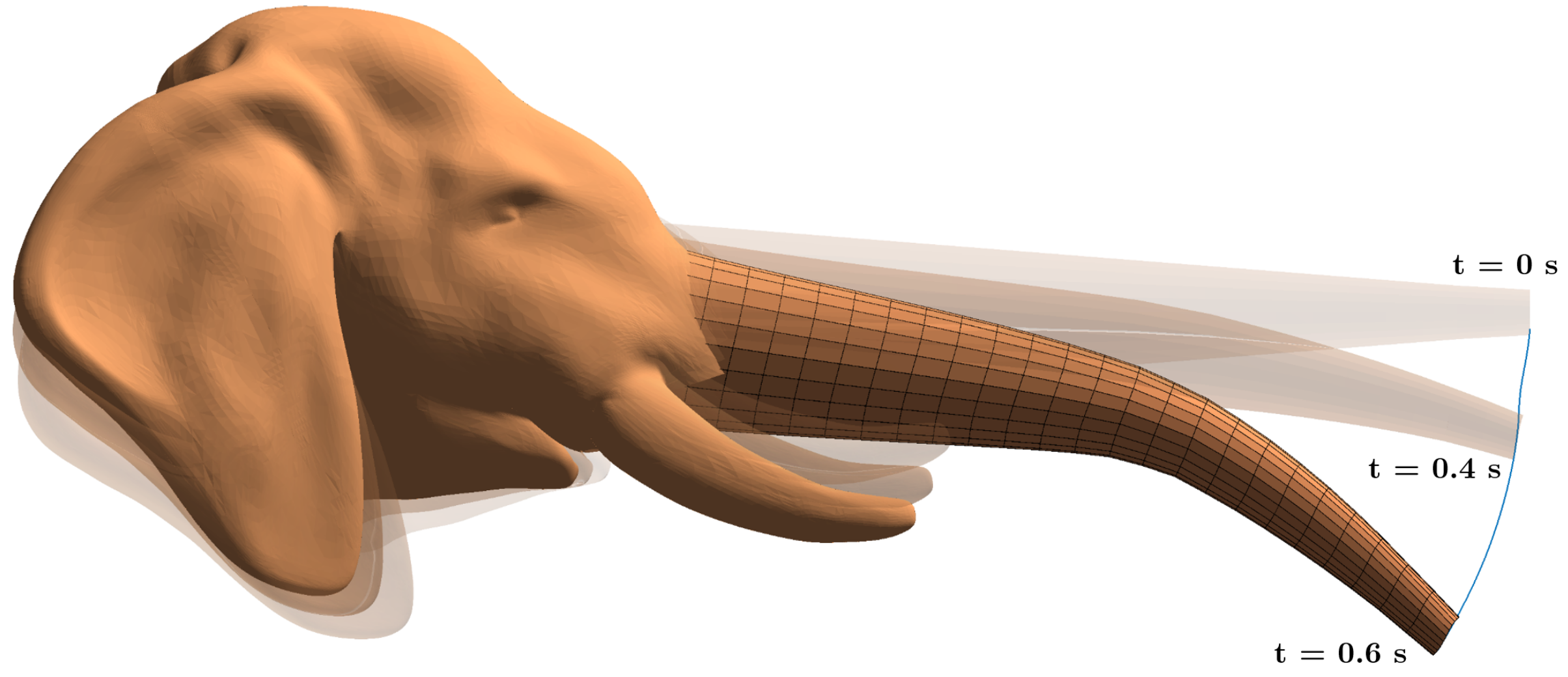
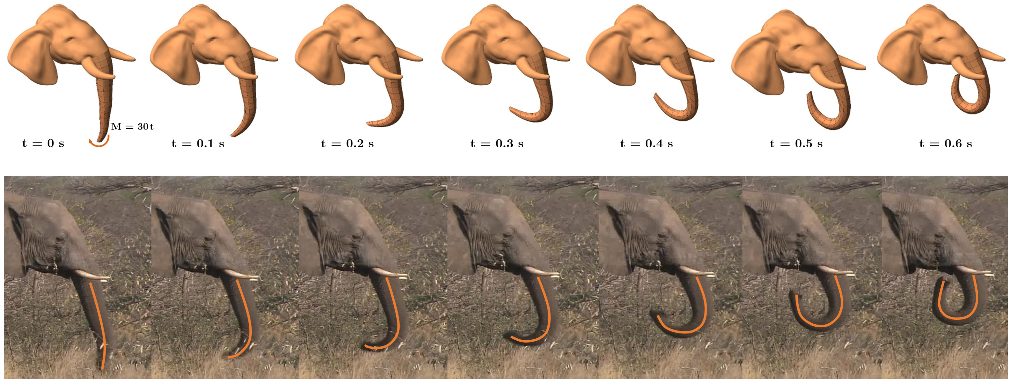
To validate the simulation and assess its accuracy, the results were compared with the actual motion of an elephant’s trunk. Figure 21 presents a side-by-side comparison of the simulated model and real trunk motion over time. To replicate the natural curling movement, a time-dependent bending moment of was applied at a point located one-quarter of the trunk’s length from the distal end, acting about the y-axis. The external force formulation described in Equation (16) was applied to the ANCF-based trunk model. Initially, both the simulated and real trunks remained nearly straight, indicating a minimal bending state. As time progressed, the trunk gradually bent, forming a pronounced curvature that closely resembled the real trunk’s upward motion towards the mouth in an active manner. The comparison demonstrates a strong agreement between the simulated and real movements, particularly in the bending pattern and temporal evolution of the curvature. This confirms that the proposed dynamic model effectively captures the natural biomechanics of an elephant trunk.
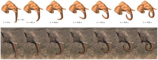
Figure 21.
Dynamic simulation of an elephant’s trunk motion along with the corresponding actual movement during feeding.
Additionally, another simulation was carried out where the system was subjected to double-acting forces to further explore the dynamic response under combined loading conditions; see Figure 22. The trunk rested in a horizontal position and was subjected to a bending moment about the y-axis, while the rigid head experienced an applied torque about the z-axis.
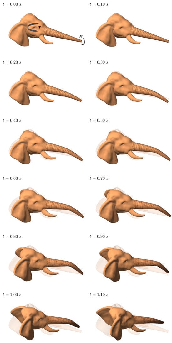
Figure 22.
Dynamic simulation of elephant’s head–trunk coupling.
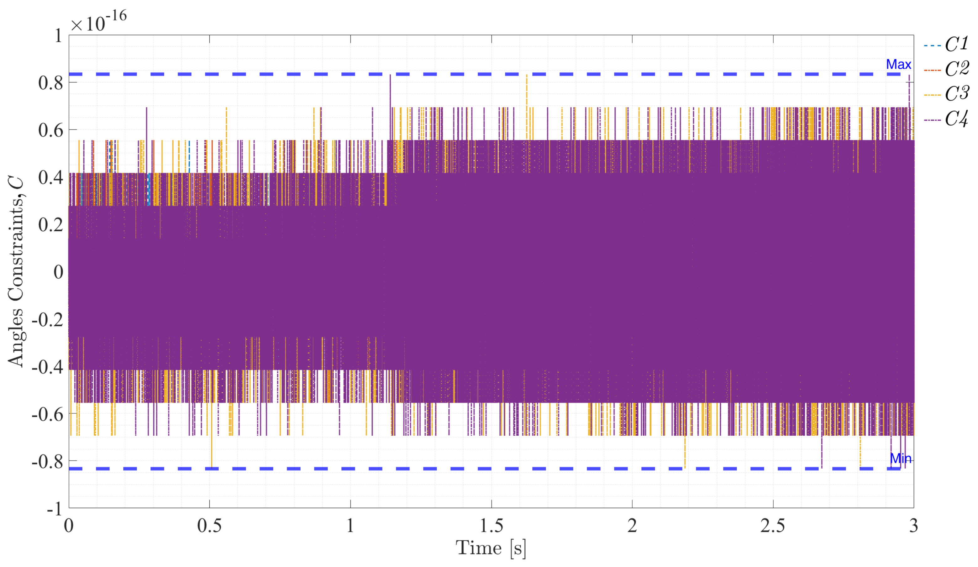
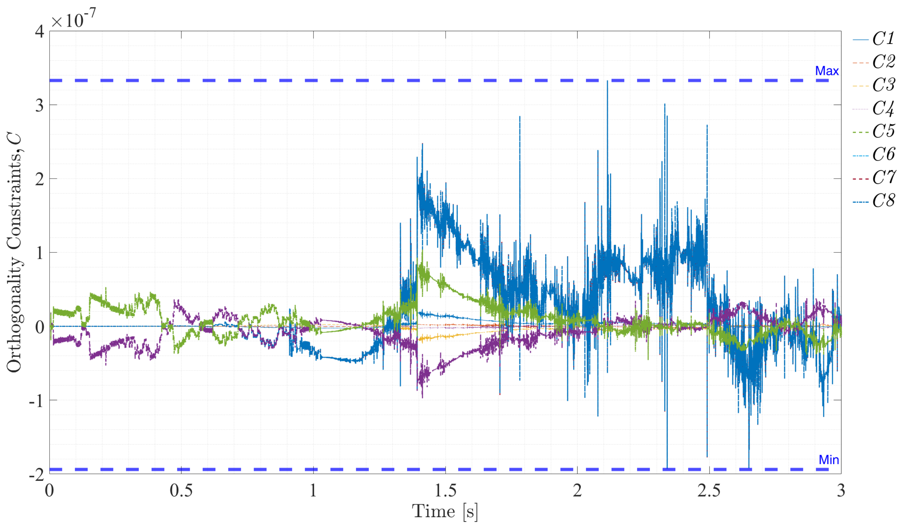
Figure 23, Figure 24, Figure 25 and Figure 26 illustrate the violations of the constraints (rigidity, distance, angle, and orthogonality) over time and demonstrate the effectiveness of the integration method and the rigid–flexible interface. For rigidity constraints, the deviations remained within , ensuring the rigid body’s behavior was accurately maintained. The distance constraints showed minimal violations, confined to the order of , confirming the precise preservation of the distance between nodes. Angle constraints exhibited negligible deviations, within , indicating the relative orientation between vectors remained constant as expected. Orthogonality constraints also displayed small violations, within , maintaining the orthogonal relationship between vectors throughout the simulation. These results collectively highlight the robustness and precision of the simulation framework, demonstrating that the system adheres to the constraints effectively over time.
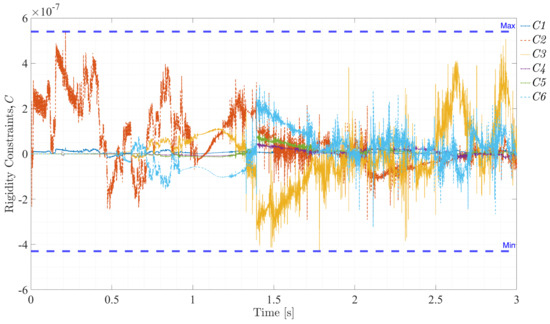
Figure 23.
Violation of rigidity constraints, Equation (7).
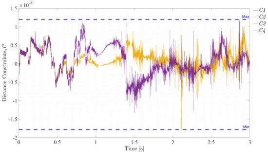
Figure 24.
Violation of distance constraints, Equation (44).
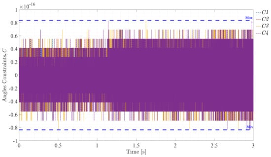
Figure 25.
Violation of angle constraints, Equation (45).

Figure 26.
Violation of orthogonality constraints, Equation (47).
It is important to note that the exact inherent damping of an elephant trunk is not explicitly documented in the literature. However, studies on elephant trunk dynamics [1,35] suggest that trunk movements rely on a combination of passive elasticity and active muscular control, both of which inherently contribute to energy dissipation. In previous implementations, the damping effect was not explicitly modeled; however, the results demonstrated realistic oscillatory behavior, ensuring consistency with observed trunk movements. The simulation approach inherently incorporates constraint stabilization techniques to manage the numerical behavior of the system. Specifically, damping in constraint dynamics is handled using the Baumgarte and Fuzzy Logic Control stabilization methods. These stabilization methods effectively regulate constraint violations, preventing unrealistic oscillations and ensuring smooth, physically meaningful motion. The effectiveness of this approach is evident in the dynamic results presented in Figure 17 and Figure 19, Figure 20 and Figure 21), where the simulated motion decay closely aligns with natural trunk behavior. Furthermore, the comparative analysis shown in Figure 21 confirms that the proposed rigid–flexible coupling model provides a reliable representation of realistic trunk mechanics, demonstrating the system’s ability to replicate natural movements observed in elephants.
8. Conclusions
This paper successfully integrated the Natural Coordinates Formulation (NCF) and the Absolute Nodal Coordinates Formulation (ANCF) to model an elephant’s head–trunk system as a rigid–flexible multibody system. The NCF was employed to model the rigid head, while the ANCF-based modeling of the trunk’s tubular structure was carried out. The NCF/ANCF model constructed captured biomechanical properties while obeying the constraints of a rigid–flexible interface and demonstrated versatility and applicability. The proposed model provides an accurate and efficient framework for capturing the dynamics of large deformations of the trunk and large rotations of the head. The Fuzzy Logic Control (FLC) constraint stabilization method was employed to ensure the robust handling of constraint stabilization, effectively eliminating drift issues in long-term simulations. Dynamic analysis showed the realistic response of the system under various loading conditions, including bending moments, applied torques, and combined forces, highlighting the intricate interplay of external forces and internal constraints. Across all constraint types, the maximum violation values were exceedingly small, which means that the rigid–flexible interface proposed in this paper, as well as the integration and stabilization methods implemented, is effective. The system adheres to the constraints over time, proving the robustness and precision of the simulation framework. These results not only enhance the understanding of rigid–flexible dynamics but also offer valuable insights for applications in robotics, biomechanics, and continuum manipulator design, paving the way for future advancements in complex system modeling. While this study focused on modeling rigid–flexible coupling dynamics, the developed framework provides a solid foundation for future enhancements. Potential extensions include the integration of active control strategies, where model-based control methods could be explored to regulate trunk movement by utilizing the system’s dynamic properties for improved adaptability and precision. Additionally, future work could incorporate soft tissue elasticity through compliant elements or reduced-order deformation models to further refine the head–trunk interaction, ensuring a more comprehensive representation of the system’s biomechanics.
Author Contributions
Conceptualization, A.N. and A.E.-A.; methodology, A.N. and A.G.; software, A.G. and M.O.H.; validation, M.O.H. and A.G.; formal analysis, A.N. and A.E.-A.; writing—original draft preparation, A.G. and M.O.H.; writing—review and editing, A.N. and A.E.-A.; supervision, A.N. and A.E.-A.; data curation, M.O.H. All authors have read and agreed to the published version of the manuscript.
Funding
This research received no external funding.
Data Availability Statement
The data that support the findings of this study are available from the corresponding author upon reasonable request.
Acknowledgments
The authors would like to acknowledge E-JUST University for providing licensed MATLAB software version R2024, developed by MathWorks, and their cooperation and supervision, provided through Professor Ayman Nada.
Conflicts of Interest
The authors declare that they have no conflicts of interest.
Abbreviations
The following abbreviations are used in this manuscript:
| ANCF | Absolute Nodal Coordinates Formulation |
| NCF | Natural Coordinates Formulation |
| FLC | Fuzzy Logic Control |
References
- Longren, L.L.; Eigen, L.; Shubitidze, A.; Lieschnegg, O.; Baum, D.; Nyakatura, J.A.; Hildebrandt, T.; Brecht, M. Dense reconstruction of elephant trunk musculature. Curr. Biol. 2023, 33, 4713–4720.e3. [Google Scholar] [CrossRef]
- Yeshmukhametov, A.; Buribayev, Z.; Amirgaliyev, Y.; Ramakrishnan, R.R. Modeling and Validation of New Continuum Robot Backbone Design With Variable Stiffness Inspired from Elephant Trunk. In Proceedings of the IOP Conference Series: Materials Science and Engineering, Novosibirsk, Russia, 12–14 December 2018; IOP Publishing: Bristol, UK, 2018; Volume 417, p. 012010. [Google Scholar] [CrossRef]
- Zhang, J.; Li, Y.; Kan, Z.; Yuan, Q.; Rajabi, H.; Wu, Z.; Peng, H.; Wu, J. A Preprogrammable Continuum Robot Inspired by Elephant Trunk for Dexterous Manipulation. Soft Robot. 2023, 10, 636–646. [Google Scholar] [CrossRef]
- Zhou, P.; Yao, J.; Wei, C.; Zhang, S.; Zhang, H.; Qi, S. Design and Kinematics of a Dexterous Bioinspired Elephant Trunk Robot with Variable Diameter. Bioinspiration Biomimetics 2022, 17, 046016. [Google Scholar] [CrossRef]
- Qin, G.; Wu, H.; Ji, A. Variable-curvature elephant trunk robot in nuclear industry. Fusion Eng. Des. 2023, 192, 113642. [Google Scholar] [CrossRef]
- Ma, K.; Chen, X.; Zhang, J.; Xie, Z.; Wu, J.; Zhang, J. Inspired by Physical Intelligence of an Elephant Trunk: Biomimetic Soft Robot With Pre-Programmable Localized Stiffness. IEEE Robot. Autom. Lett. 2023, 8, 2898–2905. [Google Scholar] [CrossRef]
- Li, X.; Zhang, S.; Xiong, Q.; Sui, D.; Zhang, Q.; Wang, Z.; Luan, L.; Zheng, T.; Fan, J.; Zhao, J.; et al. Biomimetic tapered soft manipulator with precision and load-bearing capacity. Cell Rep. Phys. Sci. 2024, 5, 102210. [Google Scholar] [CrossRef]
- Shabana, A.A. Dynamics of Multibody Systems; Cambridge University Press: Cambridge, UK, 2013; Volume 9781107042, pp. 1–384. [Google Scholar] [CrossRef]
- Shabana, A.A. Definition of ANCF Finite Elements. J. Comput. Nonlinear Dyn. 2015, 10, 054506. [Google Scholar] [CrossRef]
- Nada, A.; El-Hussieny, H. Development of inverse static model of continuum robots based on absolute nodal coordinates formulation for large deformation applications. Acta Mech. 2024, 235, 1761–1783. [Google Scholar] [CrossRef]
- Otsuka, K.; Wang, Y.; Palacios, R.; Makihara, K. Strain-Based Geometrically Nonlinear Beam Formulation for Rigid–Flexible Multibody Dynamic Analysis. AIAA J. 2022, 60, 4579–4592. [Google Scholar] [CrossRef]
- García-Vallejo, D.; Mayo, J.; Escalona, J.; Domínguez, J. Three-dimensional formulation of rigid-flexible multibody systems with flexible beam elements. Multibody Syst. Dyn. 2008, 20, 1–28. [Google Scholar] [CrossRef]
- Liu, C.; Tian, Q.; Hu, H.; García-Vallejo, D. Simple formulations of imposing moments and evaluating joint reaction forces for rigid-flexible multibody systems. Nonlinear Dyn. 2012, 69, 127–147. [Google Scholar] [CrossRef]
- Pappalardo, C.M. A natural absolute coordinate formulation for the kinematic and dynamic analysis of rigid multibody systems. Nonlinear Dyn. 2015, 81, 1841–1869. [Google Scholar] [CrossRef]
- Kaczmarski, B.; Leanza, S.; Zhao, R.; Kuhl, E.; Moulton, D.E.; Goriely, A. Minimal Design of the Elephant Trunk as an Active Filament. Phys. Rev. Lett. 2024, 132, 248402. [Google Scholar] [CrossRef]
- de Jalón, J.G.; Bayo, E. Kinematic Analysis. In Kinematic and Dynamic Simulation of Multibody Systems; Mechanical Engineering Series; Springer: New York, NY, USA, 1994. [Google Scholar] [CrossRef]
- de Jalón, J.G. Twenty-five years of natural coordinates. Multibody Syst. Dyn. 2007, 18, 15–33. [Google Scholar] [CrossRef]
- Shabana, A.; of Mechanical, D.; Industrial Engineering, U.o.I.a.C. An Absolute Nodal Coordinate Formulation for the Large Rotation and Deformation Analysis of Flexible Bodies; Department of Mechanical and Industrial Engineering, University of Illinois at Chicago: Chicago, IL, USA, 1996. [Google Scholar]
- Patel, M.; Orzechowski, G.; Tian, Q.; Shabana, A.A. A New Multibody System Approach for Tire Modeling Using ANCF Finite Elements. Proc. Inst. Mech. Eng. Part J. Multi-Body Dyn. 2016, 230, 69–84. [Google Scholar]
- Pappalardo, C.M.; Yu, Z.; Zhang, X.; Shabana, A.A. Rational ANCF Thin Plate Finite Element. J. Comput. Nonlinear Dyn. 2016, 11, 051009. [Google Scholar]
- Shabana, A.A. ANCF Tire Assembly Model for Multibody System Applications. J. Comput. Nonlinear Dyn. 2015, 10, 024504. [Google Scholar] [CrossRef]
- Jia, S.S.; Song, Y.M. Elastic dynamic analysis of synchronous belt drive system using absolute nodal coordinate formulation. Nonlinear Dyn. 2015, 81, 1393–1410. [Google Scholar] [CrossRef]
- Liu, L.; Shan, J.; Zhang, Y. Dynamics Modeling and Analysis of Spacecraft with Large Deployable Hoop-Truss Antenna. J. Spacecr. Rocket. 2016, 53, 471–479. [Google Scholar] [CrossRef]
- Luo, S.; Fan, Y.; Cui, N. Application of Absolute Nodal Coordinate Formulation in Calculation of Space Elevator System. Appl. Sci. 2021, 11, 11576. [Google Scholar] [CrossRef]
- Obrezkov, L.P.; Finni, T.; Matikainen, M.K. Modeling of the Achilles Subtendons and Their Interactions in a Framework of the Absolute Nodal Coordinate Formulation. Materials 2022, 15, 8906. [Google Scholar] [CrossRef] [PubMed]
- Chen, D.; Li, K.; Lu, N.; Lan, P. A Space-Time Absolute Nodal Coordinate Formulation Cable Element and the Study of Its Accuracy and Efficiency. Machines 2023, 11, 433. [Google Scholar] [CrossRef]
- Dufva, K.; Shabana, A.A. Analysis of thin plate structures using the absolute nodal coordinate formulation. Proc. Inst. Mech. Eng. K J. Multi-body Dyn. 2005, 219, 345–355. [Google Scholar] [CrossRef]
- Wang, T.; Mikkola, A.; Matikainen, M.K. An overview of higher-order beam elements based on the absolute nodal coordinate formulation. J. Comput. Nonlinear Dyn. 2022, 17, 1075–1091. [Google Scholar]
- Shabana, A.A. Computational Continuum Mechanics, 3rd ed.; John Wiley & Sons: Nashville, TN, USA, 2018. [Google Scholar]
- Tao, J.; Eldeeb, A.E.; Li, S. High-fidelity modeling of dynamic origami folding using Absolute Nodal Coordinate Formulation (ANCF). Mech. Res. Commun. 2023, 129, 104089. [Google Scholar] [CrossRef]
- Wilson, J.F.; Mahajan, U.; Wainwright, S.A.; Croner, L.J. A continuum model of elephant trunks. J. Biomech. Eng. 1991, 113, 79–84. [Google Scholar]
- Baumgarte, J. Stabilization of constraints and integrals of motion in dynamical systems. Comput. Methods Appl. Mech. Eng. 1972, 1, 1–16. [Google Scholar] [CrossRef]
- Flores, P.; Pereira, R.; Machado, M.; Seabra, E. Investigation on the Baumgarte stabilization method for dynamic analysis of constrained multibody systems. In Proceedings of EUCOMES 08; Springer Netherlands: Dordrecht, The Netherlands, 2008; pp. 305–312. [Google Scholar]
- Nada, A.; Bayoumi, M. Development of a constraint stabilization method of multibody systems based on fuzzy logic control. Multibody Syst. Dyn. 2024, 61, 233–265. [Google Scholar] [CrossRef]
- Dagenais, P.; Hensman, S.; Haechler, V.; Milinkovitch, M.C. Elephants evolved strategies reducing the biomechanical complexity of their trunk. Curr. Biol. 2021, 31, 4727–4737. [Google Scholar] [CrossRef]


Disclaimer/Publisher’s Note: The statements, opinions and data contained in all publications are solely those of the individual author(s) and contributor(s) and not of MDPI and/or the editor(s). MDPI and/or the editor(s) disclaim responsibility for any injury to people or property resulting from any ideas, methods, instructions or products referred to in the content. |
© 2025 by the authors. Published by MDPI on behalf of the International Institute of Knowledge Innovation and Invention. Licensee MDPI, Basel, Switzerland. This article is an open access article distributed under the terms and conditions of the Creative Commons Attribution (CC BY) license (https://creativecommons.org/licenses/by/4.0/).