1. Introduction
In healthcare modeling, especially in the context of a pandemic, it has become increasingly evident that understanding how human behavior influences disease transmission is important. Over a span of just a few years, the COVID-19 pandemic sent the world into an unprecedented health crisis, requiring extensive global efforts to combat its effects. During this period, governments and agencies were compelled to rapidly develop and adapt public health policies to address the challenges posed by the pandemic [
1]. The COVID-19 pandemic underscored the importance of understanding how human behavior influences disease transmission.
In the university setting, the role of geolocalized policies becomes evident. After the closures imposed by the pandemic, universities grappled with crucial decisions on reopening their facilities. This involved devising strategies to navigate the challenges of maintaining social distancing on campus in accordance with health regulations, thereby minimizing the risk of disease transmission. In the context of COVID-19, these strategies encompassed various aspects, including movement within the campus, social distancing in classrooms, interactions in common areas, and more. Particularly, Brooks-Pollock et al. [
2] delve into the intricacies of COVID-19 transmission within university settings, highlighting the unique challenges these environments pose. They emphasize the complex social networks and the potential for asymptomatic spread among students. Their findings reveal that, under plausible conditions, a significant proportion of students could be infected without additional control measures, especially in communal living spaces like residences. This demonstrates that simply adopting general strategies might not be sufficient. Instead, targeted measures, such as geolocalized policies, become crucial. Brooks-Pollock et al. [
2] demonstrate that controlling disease transmission within universities requires a comprehensive approach that considers not only general guidelines, but also specific patterns of movement and interaction within the campus.
Similarly, Feng and Kirkley [
3] investigate the impact of COVID-19 on individual well-being by analyzing nearly 25 million pandemic-related tweets from 20 countries and 28 U.S. states over a month. While their study does not specifically target university campuses, they underscore the importance of government actions, such as lockdowns and social distancing measures, in response to the pandemic. The study’s unique focus on geolocalized analysis suggests that this approach could aid policymakers in understanding the effects of interventions, with an emphasis on the increased use of Twitter during the pandemic. The authors propose that this methodology could assist policymakers in analyzing and monitoring the impact of interventions on the general population.
In addition, Changruenngam et al. [
4] demonstrate the role of individual human mobility in shaping the spatiotemporal dynamics of infectious disease transmission. Changruengam et al. [
4] focuses on the role of individual human mobility in shaping the spatiotemporal dynamics of infectious disease transmission. The study integrates a classical susceptible, exposed, infectious, and recovered (SEIR) individual-based model with an individual human mobility model, considering factors such as transition probabilities between localities, gravity-like components, and memory aspects. The paper explores the relationship between spatiotemporal infection spread and the landscape of human mobility, providing insights into the specific roles of human mobility in infection propagation. The analysis is conducted by considering the spread of human influenza in Belgium and Martinique as case studies.
Traditional modeling methods often encounter challenges in accurately representing how people respond to crises of such magnitude and offering tools to evaluate targeted, localized interventions to help mitigate the transmission of these diseases. Recent research has suggested that how people act in social situations is important in how a pandemic develops [
5]. For this reason, strengthening physical distancing measures within micro-communities could positively affect epidemic outcomes [
6,
7]. Therefore, it is critical to identify aspects of social conduct that could significantly influence clustering patterns in crowded places. In addition, social behavior has been successfully reproduced in a simulated environment through adaptive-learning methodologies [
8,
9,
10,
11,
12].
Agent-based Modeling and Simulation (ABMS) is a powerful tool to study epidemics and other complex systems [
13]. Namely, this technique has received considerable attention in the field of social simulation due to its capacity to represent intricate social behavior and even human emotions [
9,
14]. An agent-based model is essentially a computer program that simulates an artificial world of interacting multi-faceted agents [
15].
Reinforcement Learning (RL) offers a good opportunity for this research as it enables agents in the agent-based model to exhibit adaptive behavior in response to evolving conditions during a COVID-19 outbreak within a university campus. This adaptability enhances the realism of the simulation, reflecting the intricacies of human decision-making during a health crisis. RL is an artificial intelligence paradigm comprising mathematical methods to model goal-oriented learning and decision-making [
16]. Certainly, RL is different from other schemes, as it focuses on agent-based learning, meaning that an idealized agent interacts with its environment and learns from those experiences to achieve a predefined goal.
A central subject in Reinforcement Learning is the exploration-exploitation dilemma [
17]. Actually, the RL scheme works as a trial-and-error feedback process, where an action in the current state leads to a new state and reveals a reward, whose value is used to refine future decisions. In that sense, in each step, the agent must decide whether to explore different actions that might provide a good reward or use (exploit) a previous action that resulted in good rewards. This means the agent is not taught what actions to take; instead, it should be able to determine, by itself, what action derives satisfactory results under a particular circumstance.
Most problems in RL can be mathematically idealized according to the Markov Decision Processes (MDP) framework [
18]. Markov Decision Processes (MDPs) are a classical formalization of sequential decision-making, where the problem is framed as an extended Markov Chain [
19]. The steps involved in a typical RL method framed as an MDP generally include a sequence of discrete time steps. First, the agent performs an action
derived from the current state
and reward
. Then, a scalar reward
is received, and the agent moves to state
. Based on the last reward, the agent will determine if the previous action
was good or bad.
Q-learning is a derived Temporal Difference (TD) algorithm that is able to find an optimal policy for a learning problem framed as an MDP [
16]. The optimality condition is assured if infinite exploration time and a partially random initial policy are given. Q-learning can estimate each state’s values without demanding a model of the environment. Hence, making it especially useful for ABMS, where the emergent patterns command system behavior. Oppositely to TD, Q-learning estimates the state-action values
, which represent how good it is to perform action
in the state
. Particularly, these approximations are meant to converge to
.
Equation (
1) describes Q-learning’s update rule. Algorithm 1 describes the solution of the Q-learning scheme. All state-action value pairs are initialized with a random value in a range matching the reward signal. Then, the learning procedure is divided into episodes, which are sub-sequences of agent-environment interactions. In this paper, an episode will be conceived as a simulation run. Next, an initial state
S and action
A are selected for each episode by using an action selection method like
-greedy. An
-greedy selection chooses the best action
percent of the time and a random one otherwise. Having taken action
A, a reward
R and new state
are observed. Subsequently, the state-action value
is updated with Equation (
1) and
S is replaced with
. If
S is a terminal state, then the episode ends, and a new one is built.
| Algorithm 1: Q-learning for estimating an optimal policy [16] |
![Asi 06 00113 i001]() |
The potential of combining Reinforcement Learning with ABMS for modeling human behavior during pandemics, specifically focusing on COVID-19, is evident. Consequently, it is essential to gain insights into the dynamics of COVID-19 and its interplay with individual behavior within semi-enclosed communities like university campuses.
1.1. ABMS in Epidemic Modeling
Mathematical modeling is a fundamental tool for analyzing strategies to control the effects of an epidemic outbreak [
20,
21,
22,
23,
24]. It offers a formal structure that allows modelers to develop practical solutions to real-world problems. Numerous authors have successfully applied these methods to model outbreaks since the 16th century [
25,
26,
27,
28]. Integrating a modeling-based approach for epidemic management has improved general well-being conditions and assisted government agencies in developing effective public health policies [
28,
29].
Research on epidemiology models has focused on the development of compartment-based models [
25,
28]. In essence, a compartmental model divides the population into subgroups by fitting the disease to a natural history structure and estimating related parameters from available data [
25,
30]. Most of these compartment-based models can be solved and analyzed using simple differential equation techniques, and, as a consequence, these have proven to be very useful in real epidemic scenarios [
25,
31,
32,
33].
However, these approaches are generally very rough simplifications of an epidemic event with strong assumptions on the internal processes and homogeneous mixing of people. Additionally, these studies have commonly ignored individual heterogeneity and multifaceted interactions between individuals. They commonly assume that contacts are static and interactions are not necessarily spatially related. Moreover, there is evidence of a consensus among agent-based modelers about traditional modeling methods lacking the necessary tools to understand such complex systems thoroughly [
20,
34,
35].
Another approach for epidemics modeling focuses on the use of ABMS. Many researchers have worked to explain the emergent epidemic behavior of simple interactions within a community [
26,
36,
37,
38,
39,
40,
41]. According to Miksch et al. [
26], a significant benefit of agent-based epidemic modeling is that it allows exceptional flexibility to design very elaborate epidemic processes. For instance, Perez and Dragicevic [
35] implemented a GIS-enabled ABMS to simulate a generic city-wide epidemic incorporating attributes like gender, age, ethnicity, and many others to determine the susceptibility of different community groups. As noted by the authors, traveling individuals are more likely to be exposed, and as a consequence, the infection tends to concentrate in places like schools and universities. Later, Crooks and Hailegiorgis [
37] applied ABMS to explore the dynamics of cholera transmission in a refugee camp in Kenya. They modeled factors in family and friendship relationships and goal-oriented agent behavior for determining where to move.
Additionally, Crooks and Hailegiorgis [
37] performed a set of experiments to determine the effects of geographical interactions and concluded that geospatial setups truly determine the outcomes of an epidemic. Another example is Weligampola et al. [
41], where the authors introduce the Pandemic Disease Simulation (PDSIM) framework, an innovative ABMS that addresses the impact of the COVID-19 pandemic on diverse communities. PDSIM incorporates attributes like gender, age, ethnicity, and other individual characteristics to assess the susceptibility of different community groups to the COVID-19 pandemic. The framework allows the simulation of disease propagation, the identification of vulnerable groups, and the assessment of containment measures’ effectiveness, offering valuable insights for informed decision-making and the development of resilient and sustainable societies. All these studies support the notion that individual attributes and interactions admittedly affect the course of an epidemic.
A substantial number of studies have applied ABMS to reproduce compartmental-like behavior using the SEIR scheme. The SEIR scheme is an equation-based model that divides the population into susceptibles, exposed, infected and recovered to model how an infectious disease spreads in a closed community. The interest in modeling diseases with varying viral loads (like Dengue, Zika, and COVID-19) has increased over the last 20 years [
24,
35,
36,
37]. Most of these SEIR-based models hold a standard list of personal attributes such as age, gender, health status, and homeplace. Equally important, some of these studies incorporate common patterns such as close-proximity infections [
35], fitting probability distributions to several stages of the transmission process [
42], individual daily routines such as working and resting [
37], transportation networks [
43], and geospatial demography [
44].
Several recent ABMS studies have specifically focused on modeling the dynamics of the COVID-19 pandemic and assessing control measures. For instance, Al-Shaery et al. [
45] developed an agent-based model to investigate the effectiveness of measures like buffers, face masks, and capacity limitations in controlling COVID-19 spread during mass-gathering events. Similarly, Asgary et al. [
46] developed an ABMS tool to analyze the spread of COVID-19 in long-term care facilities. The tool uses a contact matrix based on previous research in these facilities, and accurately predicts resident deaths within a minimal variation of 0.1. Another example is Dong et al. [
47], which introduces an agent-based model designed to address the ongoing COVID-19 pandemic, particularly focusing on Shanghai’s Huangpu District. The model incorporates real-world geographic and population data, along with details of COVID-19 transmission and WHO data. It aims to simulate the virus’s spread and account for factors like population movement, detection, and treatment, as well as the impact of other similar diseases on testing resources. Through validation against official COVID-19 data, the model serves as an epidemiological risk assessment system tailored to China’s COVID-19 characteristics. It offers insights into adjusting intervention strategies and individual health behaviors, ultimately aiding in informed decision-making for effective pandemic prevention and control in China. Additionally, Jahn et al. [
48] developed a dynamic agent-based population model to compare different vaccination strategies. They found that to minimize COVID-19-related hospitalizations and deaths, elderly and vulnerable persons should be prioritized for vaccination until further vaccines are available. Sun et al. [
49] introduced an agent-based model together with a particle filter approach as a method for studying the evolution of COVID-19. With this model, they introduced a novel method for evaluating the effective reproduction number.
Given the framework of disease spread within university settings, Alvarez Castro and Ford [
50] focused on students in Newcastle University accommodation using geospatial ABMS to demonstrate how measures like face masks, early lockdowns, and self-isolation can significantly reduce infections among students. Both their research and ours use ABMS to investigate the dynamics of COVID-19 transmission within a university campus. Nevertheless, there are differences in their research focuses and principal findings. Their study primarily assesses diverse control measures within the student community at Newcastle University accommodations. Their ABMS approach effectively utilizes spatial data and mathematical epidemiological modeling to replicate disease spread, yielding consistent results with prior studies. Their research highlights the adaptability of their ABMS for regions with accessible geospatial data, offering valuable insights into high-risk locations for effective strategies. In contrast, our research emphasizes integrating adaptive learning, specifically Reinforcement Learning, to model and influence agents’ behavior during a pandemic, focusing on university campuses. While our study successfully reduces campus crowding, it emphasizes the need for comprehensive epidemic control strategies considering individual decision-making influenced by adaptive learning and targeted interventions.
Our research extends this body of work by integrating adaptive learning, specifically Reinforcement Learning, into ABMS to model and influence agents’ behavior during a pandemic, with a focus on university campuses. We highlight the importance of considering individual decision-making, influenced by adaptive learning, in developing comprehensive epidemic control strategies. While traditional compartment-based models provide a simplified representation of epidemic events, ABMS allows for more complex and realistic modeling, capturing individual heterogeneity, multifaceted interactions, and spatial relationships. This level of detail is particularly valuable in modeling diseases with varying viral loads, such as COVID-19. Therefore, using ABMS in epidemic modeling offers a powerful tool for understanding and managing disease spread, especially when it is enhanced with advanced techniques like Reinforcement Learning. By accurately simulating the dynamics of an epidemic in specific communities, such as university campuses, we can develop more effective strategies for controlling disease spread and minimizing its impact.
1.2. Adaptive Learning in ABMS
There is a growing body of literature on adaptive learning in ABMS that holds that habits and past experiences heavily influence people’s social behavior [
9,
11,
12]. Recent developments in ABMS have demonstrated the potential of adaptive learning mechanisms, such as Reinforcement Learning, to significantly enhance the modeling and simulation of epidemic scenarios [
11].
For example, Popescu et al. [
51] developed a psychology-based framework to model human emotions during disaster evacuation. Their study provides new insights into mapping emotions to membership functions so that agents act according to a probabilistic algorithm that combines personal and emotional data. In another study, Abdolmaleki et al. [
9] integrated Reinforcement Learning methods with a multi-agent system designed to simulate city fires. This research sought to create an adaptive mechanism that allows a single firefighter to learn strategies to keep people safe. Precisely, their study employed various well-known RL algorithms, including Temporal Difference, SARSA, and Q-learning.
In the context of epidemic modeling, Guo et al. [
52] developed a framework called Pandemic Control decision-making via large-scale ABMS and deep Reinforcement learning (PaCAR). It utilizes large-scale agent-based simulation and reinforcement learning to find optimal control policies that minimize infection spread and government restrictions simultaneously. It includes a realistic simulator for cities or states with vaccine settings and a reinforcement learning architecture with a reward system based on economic benefit. This framework outperforms existing methods and is adaptable to different pandemic variants like Alpha and Delta in COVID-19.
Similarly, Zong and Luo [
53] presented a reinforcement learning framework for COVID-19 resource allocation. The approach involves creating an agent-based epidemic environment to simulate transmission dynamics across multiple states. A multi-agent reinforcement learning algorithm is then developed, taking into account the time-varying characteristics of the environment. The study applies this framework to determine optimal lockdown resource allocation strategies considering factors such as population age distribution and economic conditions. Results demonstrated that this approach enables more flexible resource allocation strategies, aiding decision-makers in optimizing the deployment of limited resources for infection prevention during the COVID-19 pandemic. Kompella et al. [
54] proposed a novel agent-based pandemic simulator that, unlike traditional models, is able to model fine-grained interactions among people at specific locations in a community. Unlike traditional models, they utilized an RL-based methodology for optimizing fine-grained mitigation policies within this simulator.
Furthermore, Kadinski et al. [
55] employed machine learning in an agent-based model to propose a response and recovery approach for contamination events in water distribution systems. Kadinski and Ostfeld [
56] also proposed an agent-based model coupled to a hydraulic simulation where the decision-making of the individual agents is based on a fuzzy logic system reacting to a contamination event in a water network.
In a different context, Harati et al. [
57] used a conceptual agent-based model to simulate interactions between a group of agents and a governing agent. They included six Temporal Difference Reinforcement Learning algorithms used by the governing agent to influence the group of agents to perform an action that benefits the governing agent. Their research investigates the emergence of new social norms within an agent framework, using recognition and good reputation as incentives for agent cooperation, even without penalties. They employ ABMS to explore norm development. This demonstrates the benefits of using incentives for agent behavior and integrating adaptive learning techniques into ABMS.
In addition, in the context of ABMS for epidemic scenarios, the study by Bi et al. [
58] presented mathematical models for understanding the dynamics of human behavior during infectious disease epidemics. In their work, Bi et al. [
58] proposed two models: an Information Forgetting Curve (IFC) model and a Memory Reception Fading and Cumulating (MRFC) model. These models explored how individuals forget and relearn information about diseases and how this process affects their emotions and behavior during epidemics. The IFC model employs a forgetting curve to describe how disease information fades over time, while the MRFC model captures stochastic memory changes regarding disease information based on learning and forgetting. Their research applies these models to the 2009 H1N1 influenza epidemic, utilizing historical infection data and population characteristics to simulate its real-world impact. They stress the importance of understanding the diverse perspectives and emotions of agents in the face of disease information. Their work offers not only valuable insights into how individuals process disease information, but also provides mathematical models to analyze and simulate these phenomena. Their research highlights the significance of memory and learning processes in epidemic modeling, contributing to the growing body of literature on ABMS that examines learning mechanisms and human behavior dynamics in various epidemic scenarios.
In the same context, Augustijn et al. [
59] explored the impact of disease transmission and governmental interventions on COVID-19. Their work offers a fresh perspective in the realm of ABMS models by departing from traditional rule-based government agents and adopting Machine Learning (ML) algorithms for decision-making. In their study, governments engage in collaborative, data-driven decision processes, sharing experiences to combat disease spread. They evaluated several ML algorithms, with c4.5 and Random Forest proving effective in enhancing government risk perception. Their research underscores the potential of ML-guided government decision-making to optimize disease control efforts, complementing our exploration of adaptive learning techniques in ABMS for epidemic modeling.
In summary, the literature review provides insights into the evolving landscape of ABMS, particularly its role in understanding and influencing agent behavior within complex systems, such as disease diffusion and government interventions. Integrating Reinforcement Learning into ABMS represents a significant advancement, enabling the modeling of dynamic human behavior during epidemics. This innovation allows agents to flexibly adjust their strategies in response to changing conditions and personal experiences. It aligns with the broader application of artificial intelligence, offering promising avenues for more precise and responsive epidemic modeling and contributing to enhancing public health strategies. It is important to note that there is limited research on combining ABMS and adaptive learning techniques for modeling epidemic scenarios, with existing literature often focusing on disaster-recovery scenarios and employing artificial intelligence methods.
Existing research underscores the importance of adopting specific social rules based on agent-based learning for modeling long-term effects. While these studies provide valuable insights into social learning as a product of individual decision-making, certain aspects remain relatively unexplored. Many studies lack detailed explanations of their proposed ABMS, and could benefit from formal experimental designs featuring confidence intervals and statistical significance tests. Consequently, this study addresses these modeling gaps by employing a comprehensive experimental design that includes ANOVA tables and confidence interval analyses.
Our agent-based model encompasses three fundamental processes: daily campus routines, transmission dynamics, and adaptive learning. In the transmission process, our assumptions regarding the probabilities governing the spread of COVID-19 across the campus are derived from the existing literature, which is based on well-established research and forms the foundation for modeling how the virus propagates throughout the university campus. Conversely, for capturing human behavior within the campus, particularly daily campus routines, we draw from a combination of sources. Our approach incorporates expert opinions, data obtained from the university, and our comprehensive knowledge of the system. This multifaceted approach ensures that our model realistically represents how individuals conduct their daily activities on campus during a pandemic.
The primary objective of our model is to simulate a simplified yet informative portrayal of the COVID-19 progression, drawing inspiration from the Susceptible, Exposed, Infected, Recovered, Discharged (SEIRD)-based epidemic behavior observed in traditional models. Our model enriches this representation by incorporating geospatial characteristics of the campus, enabling us to assess and evaluate georeferenced strategies to prevent COVID-19 transmission effectively within the campus environment. We implemented a comprehensive experimental design that includes essential statistical analyses, such as ANOVA tables and confidence interval assessments.
Additionally, in this study, we employ Reinforcement Learning (RL) as a potent tool to optimize control policies within our ABMS of a university campus during a pandemic. RL allows us to establish an adaptive learning mechanism wherein agents within the model acquire the ability to make decisions based on their interactions with the environment. Specifically, RL enables us to identify and implement control policies that encourage individuals on campus to adhere to social distancing and other preventive measures. RL agents learn from the consequences of their actions, such as maintaining physical distance, wearing masks, or modifying their behavior in response to the evolving pandemic conditions. Over time, the RL agents fine-tune their strategies to maximize the objective, often focused on minimizing infections or overcrowding. This adaptive learning process is critical for optimizing control policies because it accounts for the dynamic nature of the pandemic and individual behavior. RL agents can adapt their responses based on changing circumstances, thereby improving the effectiveness of control measures. Through RL, our aim is to provide a clear demonstration of how specific control policies can be identified and applied in real-world scenarios, offering valuable insights into pandemic control within university campuses and similar semi-enclosed environments.
Our research yields significant results; we establish that RL is a robust and practical approach for effectively modeling agent behavior within the complex dynamics of a university campus during a pandemic. Furthermore, our research uncovers specific temporal patterns related to overcrowding violations, offering insights into the nuanced nature of human behavior within semi-enclosed communities. Lastly, although our adaptive learning mechanism successfully mitigated campus crowding, its impact on altering the course of the epidemic was limited, underscoring the need for comprehensive pandemic control strategies that account for individual decision-making and emphasizing the importance of targeted interventions.
The remainder of the paper is organized as follows. First, it presents the materials and methods, beginning with a thorough model description that outlines the core aspects of our research approach. Following that, we delve into the input analysis, providing insights into how we prepared and handled the data for our study. Then, we provide details on the model implementation, explaining the technical aspects of how ABMS and adaptive learning techniques were integrated. This is followed by the
Section 3, where we first delve into the details of the adaptive learning integration with ABMS, ending with the experimentation, where we explain the specific experiments conducted and the outcomes of these simulations. Finally, the paper concludes with a discussion where we assess the significance of our findings in the context of the broader field of adaptive learning within ABMS.
2. Materials and Methods
This research involves the integration of adaptive learning mechanisms into an ABMS model that simulates crowding patterns within a university campus during a COVID-19 outbreak. Specifically, the research utilizes techniques for crowding reduction based on Reinforcement Learning to enhance the outcomes of epidemic simulations within this micro-community setting. The proposed model aims to describe the effects of blending adaptive learning techniques in an agent-based model that simulates crowding patterns in a university during a COVID-19 outbreak. Indeed, the primary objective is to test whether RL-based crowding-reduction techniques can improve an epidemic’s outcome within a micro-community. Accordingly, the model should reproduce compartment-based epidemic curves to allow assessing the impact of applying adaptive learning to the forenamed curves.
The ABMS model considers the daily routines of students and university staff as they move between various campus facilities, interacting and potentially contributing to the emergence of a COVID-19 epidemic. In this model, adaptive learning refers to agents’ ability to adjust their behavior based on data gathered from their actions in the simulated environment. Essentially, each community member selects their next destination by weighing the perceived risk associated with available facilities, which relates to crowd size. This programming encourages individuals to avoid large gatherings, and as a result, each agent learns to choose routes through facilities that minimize campus congestion.
The evaluation of the model focuses on its capacity to reproduce important patterns. It aims to simulate a simplified version of the progression of COVID-19, resembling the Susceptible, Exposed, Infected, Recovered, Discharged (SEIRD)-based epidemic behavior observed in conventional models [
60]. While exact precision is not required, achieving a reasonable degree of similarity is essential to evaluate how external factors influence the course of the epidemic. Furthermore, the model should illustrate that densely populated areas result in more infections, acknowledging spatial factors such as crowding that play a role in COVID-19 transmission. Lastly, the model should exemplify how adaptive features effectively alleviate congestion on the campus, aligning with our objective to comprehend how social learning influences the outcomes of outbreaks.
2.1. Model Description
The model description in this study was designed using the Overview, Design Concepts, and Details (ODD) protocol for describing agent-based models [
61]. The overview component of our model defines its purpose, entities, state variables, and process overview. This model aims to simulate the daily dynamics of a micro-community during a COVID-19 outbreak. As a result, the agent-based model considers three core processes: daily campus routine, transmission, and learning. Firstly, the daily campus routine describes how agents move around campus following their schedule. Secondly, the transmission process explains how the disease spreads through close contact with infected individuals. Lastly, the learning process describes how people learn to avoid crowds by trial and error.
Additionally, the model has four types of entities: students, campus staffers, places, and the environment. Students and campus staff are referred to as agents. They represent real-life community members, so they emulate the epidemic interactions between individuals on campus. Each agent has a predetermined weekly routine. A routine is a set of scheduled activities an agent performs in several places. During the initialization process, each agent is assigned a plan according to its type. For instance, students follow an academic program comprising classes, laboratories, lectures, and other educational activities, while staffers follow a traditional office calendar. Following a plan means going to a facility, staying there for a predetermined amount of time, and leaving for the next activity once the current event ends.
In the campus environment, places serve as locations where agents engage in various activities or move between spots. In total, there are 87 distinct sites on the campus, encompassing a variety of types, including educational facilities, dining areas, communal spaces, parking lots, transit locations, entrances, and exits. Academic buildings make up a significant portion, totaling 23 buildings that span an expansive area of 64,624 m, considering multiple floors within each building. Additionally, there are 20 common zones dispersed across the campus, accounting for a combined area of 37,118 m. The dining areas, referred to as eating places, amount to 6 in total, collectively occupying 3821 m. Furthermore, the campus has 7 pedestrian gates for pedestrians, covering an area of 210 m. For agents moving within the campus, there are 24 transit zones available, collectively spanning an area of 11,388 m. Finally, vehicle gates are present at 7 locations, contributing to a total area of 210 m.
This information provides valuable insights into the spatial distribution and size of these diverse site types within the campus environment. At the onset of the pandemic, the country recommended maintaining a social distance of 2 m between individuals. This guideline offers a perspective on the potential capacity of these areas under pandemic conditions. For instance, strict adherence to the 2 m distancing rule implies that an open space of 100 m could theoretically accommodate a maximum of 25 individuals, assuming each person occupies a circular area with a radius of 2 m. However, it is important to recognize that the actual capacity of these areas may be lower due to factors like room geometry, the presence of entrances and exits, and the need for pathways to facilitate movement. Determining the capacity of these areas under social distancing guidelines is a crucial consideration when planning campus operations and activities during the pandemic.
The description of these places is fundamental to estimating the population density at each simulation step. Also, agents walk through or stay at these places, depending on their routine. Finally, the environment is a single entity that keeps track of the simulation and controls when the outbreak starts. Explicitly, this entity manages global behavior and, therefore, is critical to perform the experiments.
Table 1,
Table 2 and
Table 3 describe the state variables of the agents, places, and environment, respectively.
The proposed model utilizes two-dimensional GIS polygons to represent the spatial layout. Consequently, agents interact within an environment resembling the reference campus’s scale. This results in spatial dimensions having a nearly 1:1 relationship with real-life proportions. The simulated university encompasses an area of approximately 130,000 m, chosen to mirror the actual campus dimensions in Medellín, Colombia. In contrast, each time step corresponds to one hour, and the simulations run for a duration of 150 days. This temporal extent was chosen to provide ample time for simulating an epidemic that could potentially affect the entire campus population.
A student’s day schedule can be described as follows: The Students arrive at a campus entrance, update their current location, and then proceed to their next academic activity by taking the fastest route available. During this time, students inform each visited place to update the population density and count of people present. While participating in an event, students remain in the facility, and upon its conclusion, they decide on their next course of action. This involves either relaxing in a common area or proceeding to their next activity. The decision to have lunch on campus is predetermined during initialization, so if a student chooses to dine on campus, they select an eating location, have their meal, and depart upon completion of the meal. After completing all daily activities, students head to a random exit for their journey home.
The schedule for the staff is similar to that of students. On weekdays, staff members arrive at a campus entrance, update their current location, proceed to their workplace, work until noon, and then have lunch. Subsequently, they return to their office and continue working until the end of their shift. At the end of the workday, staff members head to a random exit to make their way home.
The transmission process describes how COVID-19 spreads throughout the campus. At the beginning of the simulation, the environment entity schedules the occurrence of the first active case. In this scenario, a randomly selected individual is marked as infected, and their compartmental state is updated accordingly. Infected individuals follow their usual routines, with the distinction that they can potentially expose nearby susceptible individuals to the disease. When an infected agent comes into close proximity with a susceptible community member, a random process determines whether the contact results in infection. If successful, the exposed individual is categorized as exposed. Subsequently, another random process establishes the current stage’s duration and schedules the infected state’s assignment. Additionally, the agent notifies its current location to update the infection count. Eventually, the agent becomes infected and can potentially transmit the virus to others. Furthermore, a stochastic mechanism determines whether the agent succumbs to the infection or becomes immune, scheduling the corresponding state update.
2.2. COVID-19 Transmission Process
Our study uses the COVID-19 pandemic as a case study. Our primary motivation is not to provide a precise representation of the disease but to offer a simplified and informative illustration of the progression of COVID-19. The model is inspired by conventional models based on the Susceptible, Exposed, Infected, and Recovered (SEIR) framework. It is guided by the existing literature available during the early stages of the virus’s emergence, and our assumptions are grounded in established research, shaping our understanding of how COVID-19 spreads across a campus.
When representing human behavior in daily campus routines, we adopt a comprehensive approach that amalgamates insights from experts, data from the university, and our proprietary system knowledge. This multifaceted approach ensures that our model faithfully replicates human behaviors during a campus-based pandemic scenario, considering a range of influential factors.
It is important to note that models based on differential equations that govern transitions between states, such as the SEIR ODE-based model, provide a broad overview of disease spread. However, they operate under the assumption of homogeneity within each compartment, and they do not explicitly model interactions among individuals. In contrast, our ABMS is a more intricate and nuanced model that simulates the actions and interactions of independent agents to evaluate their collective impact on the entire system. This approach considers spatial factors and individual behaviors, leading to more precise and context-specific predictions.
This paper focuses on simulating how a COVID-19 outbreak progresses inside a semi-enclosed community. Several authors have pointed out that the compartmental SEIR scheme furnishes a satisfactory structure for modeling the disease under study [
62,
63,
64]. Evidence reveals that COVID-19 involves an exposure stage where the individual holds the virus but cannot transmit it to others [
65]. Consequently, the examined sickness is abstracted as an infectious disease that can be explained through five independent compartments. In particular, individuals are classified as either Susceptible (S), Exposed (E), Infected (I), Recovered (R), or Dead (D).
In our model, every agent holds an internal mechanism that controls its disease’s stage. At the start of the simulation, most individuals are susceptible, meaning they are vulnerable to COVID-19. Either they have not been exposed to the virus so far or have such a low viral load that is unrepresentative of its condition. Suppose a susceptible subject meets an infected community member within a small radius. In that case, the former is more likely to be exposed. In essence, exposed individuals are agents that contracted the disease but are currently incapable of disseminating it. However, newly exposed individuals will become infectious in a matter of days, according to the distribution of the latency period. Certainly, infected people can either die or survive, as it greatly depends on the patient’s condition. Discernibly, this epidemic system and related agent interactions are assumed to be governed by random processes that can be fitted to probabilistic distributions. The selected COVID-19 transmission process is based on the first strain of the SARS-CoV-2 virus presented in
Figure 1. All the transition probabilities between states that we use in our model are based on the literature available at the time of this study and are described below.
An essential aspect of the COVID-19 transmission process is the probability of exposure due to close contact with an infected individual. As suggested by He et al. [
66], this component is included in our model as the likelihood of a
distribution with parameters
,
, and
described in Equation (
2). The proposed approach designates that the exposure progression rate
is a function of the time the infected subject has been able to spread the virus. The recommended distribution uses a shift parameter
, because evidence shows that virus carriers can spread the virus up to 2.4 days before symptoms’ onset [
66].
Another critical feature in the representation of the epidemic process is the latency period. The latency period is defined as the time interval between an individual being exposed and later being capable of spreading the virus to others [
67]. He et al. [
66] indicate that spreadability is proportional to the appearance of the first symptoms. Accordingly, we assumed in our model that this period can be specified in terms of the incubation period (time between the exposition and symptoms’ onset) by shifting it 2.4 days to the past. In addition, Lauer et al. [
68] estimate the distribution of the incubation period as a
distribution with parameters
and
, as depicted in Equation (
3), which is the distribution that we considered in our model.
Figure 1.
COVID-19 transmission process [
66,
68,
69,
70,
71].
Figure 1.
COVID-19 transmission process [
66,
68,
69,
70,
71].
As previously mentioned, at the time of this study, it was assumed that an infected individual would either die or make a full recovery, with the latter resulting in complete immunity. Additionally, when an agent becomes infected, a random process is employed to classify the agent into a specific patient type. This classification plays a crucial role in determining future outcomes, considering the well-established fact that COVID-19 affects individuals differently. In our model, we use the patient classification based on the severity proposed by Ferguson et al. [
69]. Following the cited grading, infected agents are categorized according to empirical probability
, as shown in Equation (
4).
Once a patient type is assigned, the simulation must determine whether the agent will survive or not, and schedule the corresponding event. In fact, Liu et al. [
70] state that the severity of symptoms influences mortality. Considering that, we assumed, based on Liu et al. [
70], that the death rates are 15% for patients with severe symptoms and 50% for critical subjects, as shown in Equation (
5).
It is assumed that neither death nor recovery follows a constant time duration after infection. Instead, the time until discharge is considered a random variable with positive values. To address this, we conducted a goodness-of-fit test using the Kolmogorov–Smirnov test based on patient records from Xu et al. [
71]. The resulting distribution is presented in Equation (
6).
Certainly, understanding the disease dynamics of COVID-19 highlights ABMS potential for modeling disease transmission. ABMS ability to represent social interactions, individual decision-making, and system-level behaviors makes it an excellent tool in epidemic modeling.
In developing our ABMS and detailing its components, we have aimed for a comprehensive representation of a micro-community during a COVID-19 outbreak. Our adherence to the ODD protocol for model description ensures that we have considered key aspects of the system, encompassing daily routines, disease transmission, and the learning process. Our model provides a faithful representation of a real-life campus, considering various places and their spatial distribution. Notably, the model’s scale closely matches the physical dimensions of the actual campus in Medellín, Colombia. We have meticulously calibrated the temporal aspects, with each time step corresponding to an hour and the simulation running for a duration of 150 days, which provides ample time to capture the dynamics of a potential epidemic across the campus. Through our model’s implementation, we have strived for a realistic portrayal of students’ and staff members’ daily schedules and interactions, capturing the essence of a campus community’s activities. The transmission process, which models how COVID-19 spreads, accounts for interactions, potential exposure, and disease progression, ensuring that our results reflect plausible scenarios. The initial introduction of COVID-19 cases into the simulation aligns with actual disease progression scenarios.
An important aspect of our work is the validation of the conceptual model and simulation outputs. We engaged with university experts to scrutinize our model and its results, ensuring that they are representative and plausible. This validation process further strengthens the credibility of our ABMS, providing a reliable representation of the demographic realities on campus during a pandemic.
2.3. Input Analysis
In this section, some components related to input parameters and data sources used in our ABMS model will be presented. The parameters of the ABMS are listed in
Table 4, with each parameter being accompanied by a brief description, measurement unit, and default value.
In addition to the input parameters, several data files from external sources are also required to run the model. For instance, shapefiles (.shp extension) are needed to build the campus geography inside the GIS projection. Specifically, these files contain a geometrical representation of each one of the facilities in the simulation. Moreover, additional CSV files are expected that characterize each of the available amenities’ attributes. In particular, each place holds an ID, an area in square meters, a state that determines if the site is currently active or not, and a link to another location in case it is required. Furthermore, another file is needed to select the areas that correspond to workplaces, as each staffer will be assigned to one of those.
Moreover, a supplementary routes file is mandatory, as it defines how facilities are connected to each other in a network structure. As previously mentioned, agents walk around campus to their selected next location, meaning they must pass by different places to reach their final destination. That is why, to simplify the traversal process, a graph-based structure was designated. The regarded graph is built by taking the facilities as nodes and the distance between them as arcs. On top of that, Dijkstra’s algorithm is used to find the shortest route between an origin and a destination.
Similarly, a group’s file is also compulsory. This file contains the academic schedule to use as a reference for the student’s routine. Particularly, the program comprises subject groups, each featuring a subject ID, a day of the week, a start time, an end time, a student capacity, and a facility. The idea is that a student enrolls in several groups, determining what he or she must do during the week.
It is important to note that not all agent behaviors in our model rely on data; some involve estimating important parameters based on expert insights and available information about the variables. For instance, certain processes lacked specific data, such as the duration of lunch breaks in the cafeterias and the timing of the lunch period. We gathered estimated values through stakeholder consultations and interviews with logistics personnel in these cases. Stakeholders reported an estimated mean duration of 45 min for lunch breaks, ranging from 15 to 75 min. Logistics personnel interviews indicated a typical midday meal time frame from 11:30 am to 2:00 pm. A similar approach was applied to model several other secondary processes, utilizing input from Universidad EAFIT’s staff. However, when data were available, we conducted fitting procedures using Goodness-of-Fit tests.
Table 5 summarizes the main stochastic elements in the model. We use a Bernoulli distribution with an unknown parameter
p to determine whether a community member arrives on campus in a vehicle; this is relevant as car entrances differ from pedestrian ones. Parameter
p is set as a model input parameter because different car-based restriction scenarios will be evaluated in future works. In addition, a uniform walking speed in meters per minute is defined in the 70 to 100 limit, as it renders a lower and upper bound of reported velocities for different age ranges [
72].
2.4. Model Implementation
Our ABMS model was implemented in the Repast Simphony platform, an open-source framework for simulating agent-based systems. We use Repast Simphony Version 2.7 on a 4-core Windows machine with 8 gigabytes of RAM and a speed of 1.5 GHz. Repast Simphony is based on object-oriented programming principles and provides a broad toolkit for effectively modeling and analyzing dynamic systems. Its open-source nature allows collaboration with other modelers, and compatibility across different operating systems is ensured by its Java-based design. Moreover, organized and modular model development is facilitated by Repast Simphony, which is deemed essential for complex simulations. The platform’s scalability accommodates simulations on various scales. For a broader overview,
Figure 2 presents the components of our model, and
Figure 3 exhibits a rough blueprint of the syndicated classes and their interactions. Note that, In
Figure 3, the asterisk (∗) symbol is used to represent multiplicity in a relationship between two classes. Multiplicity indicates the number of instances of one class that can be associated with instances of another class.
The ABMS is divided into seven modules, each one of them responsible for a specific task. The central module, simulation, is in charge of orchestrating the model’s execution. Plainly, the aforementioned building block interacts with other peer constituents to set up the model and manage scheduled events. On the other hand, one of the initial configuration tasks is loading all the necessary data, which is, by the way, the data loader module’s job. Pointedly, the former module is in command of accessing external data sources and transforming them into Plain old Java objects (POJOs). Once the bootstrapping ends, the simulation instantiates all the agents, in this case, all students, staffers, and locations.
The agent behavior unit operates how agents interact with each other and with the environment. In detail, the antecedent module is responsible for enforcing each community member’s daily routine. On the side, the natural history artifact guides disease dynamics. As mentioned before, one of its primary inputs is the patient type, an internal attribute every individual holds, as infected subjects are classified in accordance with the severity of their symptoms.
Moreover, all those previously discussed agent interactions, behaviors, and internal mechanisms are present in a simulated geospatial environment. As previously stated, facilities are materialized into polygons. The GIS-enabled environment supports the integration of a weighted-graph-based structure that emulates on-campus routes. The geography management module supports all the earlier features. Last but not least, the learning and output management modules are self-explanatory under precedent descriptions. Conversely, seamless orchestration is the key to success. Each module might work independently from others, but its dependencies allow for contract-based synergies that enable strait-laced modularization and low coupling.
Initialization refers to the process that sets up to model before its actual simulation. In this case, this ABMS requires several initial steps before it is ready to emulate the campus dynamics. At initialization, the different types of agents are created according to the parameters described in
Table 4. First, the program reads all shapefiles and extracts the corresponding GIS polygons to build the facility agents. Each place entity is generated by reading both its associated shape and attributes file. Once all sites are instantiated, the simulation builder reads the workplace file to keep references to the office locations for later usage.
After forging all site agents, the routes file is read into a weighted graph structure. Recall that the nodes represent locations on campus, and edges refer to distances between those places. Now, suppose that the routing algorithm is embedded into the agents, meaning that each time a student wants to go to a specific location, it is responsible for calculating the fastest route to its destination. In reality, the foregoing approach is impractical, as it is very likely that lots of agents will need to calculate the same paths repeatedly. That is why an initial procedure is implemented to calculate the shortest route between all possible localities. Found courses are stored in a hashed map with unique keys that designate the origin and destination pair. The proposed method is sketched in Algorithm 2.
| Algorithm 2: Calculation of shortest paths between localities |
![Asi 06 00113 i002]() |
Following route building, the program loads the group’s file into a collection of objects. Later, student agents are produced according to the simulation parameters. Remember that two sets of students are created: the initial susceptible and those that will become infected once the outbreak is activated. The specifics of the student initialization will be discussed in a bit. In the meantime, as soon as the application holds a list of students, it continues by assigning them a schedule according to the previously read academic plan. The foretold assignment was designed to be straightforward, with no intricate heuristics to balance the student population, as it was deemed unnecessary. Precisely, schedules are allotted randomly. Outright, a random number of groups to enroll
n is generated for each agent according to the Binomial distribution in
Table 5. Then, the algorithm shuffles the groups’ list and selects
n arbitrary groups with at least one available spot if that is possible. If the affirmative case, the student is enrolled in the mentioned course. Otherwise, if no single group is attached, the agent is removed from the simulation. The suggested randomized procedure is outlined in Algorithm 3.
| Algorithm 3: Student’s schedule assignment |
![Asi 06 00113 i003]() |
The staffer agents are immediately materialized and added to the simulation context. At this point, all agents have been embodied, though a few inner details were left undisclosed. For instance, how the internal features of each agent type are initialized. To all intents and purposes, all community members are made ready as follows. First, the vehicle usage attribute is fixed according to the Bernoulli distribution in
Table 5. Next, if the individual was marked for spontaneous infection, the corresponding transition is programmed to comply with the outbreak tick parameter in
Table 4. Later, the learning mechanism is turned on, and the state-value pairs are set to their initial values. Afterward, the agent is sent home to an undetermined location outside the campus. Finally, all weekly recurring events are timetabled in line with the agent’s type.
Weekly recurring events are a core component in the model under examination. The prior is true because the ABMS was coded in an event-based fashion, where agent interactions are orchestrated through a prearranged set of repeating events. As a rule, the following four types of activities are anticipated: academic or work-related ones, the arrivals to campus, the departures to home, and having lunch. These are implemented separately for the students and staffers, as they hold dissimilar routines. Namely, students arrive on campus according to their assigned schedule, showing up a few minutes before their first academic activity. However, staffers arrive close to 7:00 a.m., at the start of the working shift. Similarly, students return home after their last activity, whilst staffers have a pre-established exit hour.
During the model’s development, a visual aid was implemented for illustration and shallow validation purposes in the form of a 2D geo-map.
Figure 4 presents the forenamed graphical representation of the model’s workings. Respectively, the mentioned depiction is remarkably appropriate for observing global behavior such as crowding and outbreak progression. To be specific, blue dots symbolize susceptible individuals. Colors change as the disease proceeds to orange for exposed, red for infected, green for recovered, and black for dead.
3. Results
In this section, we present the outcomes of our research, investigating how reinforcement learning impacts social distancing on a simulated campus and, by extension, its influence on the spread of COVID-19. Our main objective was to determine if RL-driven adjustments in behavior could effectively reduce crowding on campus and potentially mitigate the virus’s transmission. Having discussed the theoretical foundations and detailed our experimental setup in previous sections, the focus is now on integrating RL-based adaptive learning into the ABMS model. Additionally, we evaluate the influence of this adaptive learning on campus density and the evolution of the COVID-19 outbreak within our simulation scenarios. We analyze the effects of different RL parameters, such as learning rate (), exploration probability (), and discount factor (), on key metrics like campus density and epidemic dynamics. Through rigorous statistical analysis, we assess the practical implications of these findings, shedding light on the potential of RL-based strategies to reshape social behavior during a pandemic.
3.1. Adaptive Learning Integration with ABMS
In this subsection, we go into the specifics of the adaptive mechanism we have employed. It is important to recall that our aim with this mechanism is to facilitate agents in learning social distancing behaviors while preserving the normalcy of campus life. We operate under the assumption that individuals within the community are rational and prioritize avoiding infection. This inherent drive motivates them to adapt their behaviors to minimize exposure to potential risks willingly. It is important to note that in our scenario, agents act solely based on their personal experiences and not due to external influences.
Our chosen learning approach is grounded in a Q-learning scheme with -greedy action selection. We opted for this strategy due to its adaptability, versatility, and ease of implementation. Among the various tabular methods we explored, Q-learning offers a straightforward method for estimating state-action values and is well-suited for navigating a dynamic environment comprising thousands of knowledgeable agents vying for limited resources. Each agent operates independently, mirroring the concurrent adaptation of a small-sized community within the simulation.
There are four fundamental components in our proposed design. Firstly, we have the representation, which defines what states, actions and values signify. Secondly, initialization outlines how the scenarios are set up initially. Thirdly, action selection elucidates the process of choosing the next action in the current state. Lastly, value update elucidates how estimations are revised based on the reward signal. Regarding representation, states correspond to specific locations on campus, with each state representing a distinct available location to visit. Actions, on the other hand, symbolize the act of moving from one location to another. The value associated with a state–action pair indicates the desirability of selecting a particular destination while currently situated in another place. Consequently, the value function is modeled as a lookup table comprising entries, where ’s’ represents the state and ’a’ denotes an available action.
Only the following amenities are considered in the learning process: teaching facilities, common areas, and eating places. It is evident that there is a vast amount of Q values as locations are taken in pairs. On the subject of initialization, preliminary experiments suggested the best setup was leaving all initial figures at zero, thus implying that all places have the same attractiveness factor in the first iteration. The referred situation does not match the classical scheme that recommends a random initialization procedure.
An -greedy strategy was implemented in the matter of action selection. The idea behind this procedure is that actions should be picked considering the exploration–exploitation dilemma. To be exact, the best available action, referring to the one with the highest Q figure, is selected with probability , while a random one is chosen in the opposite case. By way of explanation, the examined method is sketched in Algorithm 4.
Regarding the Q values’ update, a reward signal was picked to outcome positive figures for safe places and negative amounts for sites that exceed the ideal social distancing measure (as described in
Table 4). The proposed payment for landing in a certain location is described by Equation (
7), where the social distancing is measured in meters, and the current density of the place is estimated as the number of people in that location over its superficial area in square meters. As an illustration, if the social distancing policy is set to 2 m, then densities over the 0.5
mark will be considered threatening.
| Algorithm 4: -greedy action selection |
![Asi 06 00113 i004]() |
Considering the four preceding ingredients, the learning scheme can be summarized in Algorithm 5. Essentially, adaptation only happens when the agent faces site selection circumstances. It is crucial to clarify that the convergence of the algorithm greatly depends on the parameter configuration, as careful attention is required to balance the exploration-exploitation dilemma [
16]. For that purpose, a three-factor factorial design of experiments is applied to analyze each parameter’s effects. Despite everything, results are expected to show different outcomes, good or bad, under each scenario. Anyhow, the intention was not to reveal pleasing results in all examined situations; instead, the idea is to identify the key differences under various settings.
| Algorithm 5: Q-learning scheme for crowding reduction |
![Asi 06 00113 i005]() |
In order to assess the influence of the implemented RL-based adaptive features, a base scenario is defined. The selected reference settings render a population of 10,000 students and 200 staffers and fix both the infectious radius and social distancing measure to 2 m. Additionally, we use a uniform random procedure to select facilities (similar to an
setup). Therefore, the picked parameter values are the same as those reported in the default value column in
Table 4. However, remember that learning parameters
,
, and
have no effect at all in the course of the earlier described scenario. For descriptive purposes, mean on-campus densities for ten repetitions are shown in
Figure 5.
Figure 5 reveals recurrent patterns of density peaks over the 0.5
threshold, which indicates that the current crowding dynamics do not comply with recommended social practices. However, a more in-depth analysis is required to identify the temporal fragment that poses the greatest threat to the community. Next, some descriptive statistics for the density output are reported in
Table 6.
Table 6 shows that the mean density on campus is around 0.10 people per square meter, meaning that agents are 10 m apart on average. Still, the median value is utterly different from the aforesaid measure, suggesting the presence of outliers. Yet, anomaly detection techniques are not applicable here as the outliers are of special interest in the analysis. Having said that, the recorded high skewness value exhibits a significant positive asymmetry. Simultaneously, the kurtosis figure displays a slight tendency of greater deviations to the mean that conforms with previous findings. In summary, computed metrics agree that density values are not homogeneous and that outliers’ demeanor is meaningful. Along with it, a histogram of densities is plotted in
Figure 6 according to Sturge’s criteria.
As expected, the histogram in
Figure 6 provides further details on the distribution of the density figures. For instance, around 60% of the measurements are lower than the 0.1 people per square meter mark, while only 0.9 percent of the values are actually larger than the social distancing measure. In simpler terms, results show that potentially dangerous situations happen less than 1% of the time.
For good measure,
Figure 6 could raise some doubts about the densities’ distribution, since the graphic may lead to thinking that these could be drawn from a mixing of two random variables. One way of making sure that results are legitimate is by means of an analysis of independence. By this study’s standards, the densities should follow some foreseeable structure, given that gatherings are based upon the academic schedule. Due to this, an overlapped scatter plot should evince non-random patterns, and an autocorrelation plot is likely to exhibit substantial correlations for some lag values.
Figure 7 conveys the previously mentioned diagrams.
Unsurprisingly,
Figure 7 clearly demonstrates that the data densities are not random. Specifically,
Figure 7a visually depicts the sequential arrangement of data points and illustrates the relationships between each data point and its neighboring point. Therefore, as the data exhibits a linear tendency, this plot effectively highlights the non-random nature of the data densities. Similarly, in
Figure 7b, the autocorrelation between each data point and its preceding data points is visually represented. Autocorrelation values span from 1 to −1, denoting positive or negative correlations, respectively. Notably, the figure displays autocorrelation values approaching either extreme, indicating the existence of autocorrelation within the dataset and confirming the non-random nature of the data densities.
To continue with the analysis, two box-plots are brought into the examination to browse how densities behave in various temporal groupings.
Figure 8 presents the above-stated charts. A closer inspection of
Figure 8 shows noticeable differences between the examined temporal partitions. For instance, it is apparent from the figure on the left that weekends’ densities are almost negligible. Additionally, Friday’s quantities do not exceed the 0.35 bar, implying that unfavorable gatherings are not likely to occur from Friday to Sunday. At the same time, Monday to Thursday’s maximum measurements are close to the 0.5 benchmark, with the highest values being recorded on Tuesdays. Setting aside, the figure on the right shows that bigger congregations happen close to lunchtime, where most agents look for a place to eat in one of the few available. Other distinctive top figures are seen near common arrival and departure times, suggesting that agents crowd in places near the entrances and exits at these time frames. Altogether, the evidence suggests that Tuesdays close to lunchtime deliver the utmost risk of clustering. For a proper validation of the last statement,
Table 7 presents the mean confidence intervals for the densities each day and in the whole week.
The evidence in
Table 7 supports that Tuesdays hold noticeably larger gatherings than any other day of the week. Now, in relation to the comparison with the implemented learning method, a reference densities curve should be selected. In this case, the maximum weekly density time series is picked, the reason being that it suppresses the effect of the weekend figures and allows for a smoother comparison with experimental results.
Figure 9 displays the aforementioned data points on the right.
What is interesting about the data in
Figure 9 is that maximum densities seem to shift randomly near the 0.55 yardstick up to the 80th day. Then, the specified figures go down slightly and converge near 0.53. Noticeably, the above behavior matches the scheduled outbreak progression, since it starts at day 60 and should begin reporting dead cases in the following 15 to 20 days. The differences suggest that the epidemic itself reduces the maximum crowding values by 0.02, which is not meaningful at all.
Base epidemic outcomes are showcased in
Figure 10. It is apparent from the graphic that broad compartmental dynamics hold because the manifested behavior resembles a classical SEIRD scheme. Despite that, notable differences are revealed, since irregularities are detected in the susceptible and exposed curves. The results are quite revealing in several ways. First, a peak of 9424 infected subjects on day 20 conveys that COVID-19 progresses astonishingly fast in a semi-enclosed community where no action is taken, recording a 0.92 prevalence rate in a couple of weeks from the initial case. Second, a 3.9% mortality rate is registered, comparable to recently reported fatalities ratios [
73]. Finally, a rather odd phenomenon is observed in the exposed curve, as the data does not follow a bell-shaped form; more precisely, exposed cases break in the middle and go up a few days later. The last proceeding could be explained by the latency term being around 2.4 days shorter than the incubation period and no new infections appearing on weekends.
Robinson [
74] states that multiple replications are required to obtain a good enough estimate of a model’s mean performance. Unequivocally, a central question is: how many simulation runs must be performed? A rule of thumb hints that at least five repetitions should be carried out. However, a precise derivation is preferred instead. For instance, a statistically reliable method involves rearranging the confidence interval formula, as shown in Equation (
8), where
X is the variable of interest,
is its expected value,
is its estimated standard deviation,
is the selected significance level, and
d is the percentage deviation of the confidence interval about the mean. Now, taking the maximum weekly density as the variable under study, a significance level of five percent (
) and a deviation of ten percent (
),
minimum replications are obtained. Therefore, at least six simulation runs are recommended per experiment. Indeed, that means that the initial ten runs are sufficient.
3.2. Experimentation
The preceding results show that the learning-lacking scenario does not comply with the social distancing policy. Thus, a design of experiments is aimed to determine the effect of RL-based social distancing with different sets of parameters. Truly, it would be ideal to examine a vast array of parameter settings. Still, extensive simulation times constrain the number of trials to perform in a reasonable time and with limited computing resources. Consequently, a
factorial design is chosen, where
k is the number of factors to analyze. Specifically,
factors are considered according to parameters
,
, and
.
Table 8 presents the figures selected as the low and high levels for each experimental factor.
The factors’ levels were selected intuitively following their effects. Namely,
was assigned a 0.1 low level, as smaller values will likely lead to imperceptible corrections and a 0.25 high level as larger figures could potentially head to oscillatory behavior. Similar arguments were examined while choosing the bounds of the remaining parameters.
Table 9 describes the proposed
factorial design.
The experiments were repeated six times, as previously stated, to capture the variability of the model’s outcomes up to a 10% confidence interval deviation from the mean. Remarkably, results show that agents are absolutely capable of learning to avoid crowds on campus, thus, validating the hypothesis that the suggested RL-based approach is suitable for implementing the adaptive learning mechanism. As expected, maximum weekly densities reduce progressively while agents accumulate experiences in their daily activities.
Figure 11 exhibits the mentioned behavior.
Figure 11 contrasts the base scenario with the eight experiments. What is striking about the outcomes is that all parameter settings significantly reduce maximum weekly densities with respect to the base case. Notwithstanding, some scenarios provide better results than others. For example, Experiment 2 affords the greatest decline in supreme densities and ends up in a situation where on-campus gatherings are, on average, below the 0.40 mark (10 points below the recommended social distancing policy). Extraordinarily, all experiments render a behavioral shift that positions the community in a sweet spot regarding compliance with the minimum physical distancing measures.
Table 10 displays some relevant density figures for each one of the scenarios.
What stands out in
Table 10 is that the experiments with the highest relative reduction in the maximum weekly densities (Experiments 2 and 6) share the same parameter values for
and
. All in all, evidence suggests that the second setup is a local optimum with respect to the chosen experimental space. Nevertheless, the aforementioned settings are not guaranteed to be a globally optimal selection of learning parameters. Undoubtedly, a more in-depth optimization procedure is required to establish the Pareto set of learning factors to procure the maximum decline in density figures. Having said that, the obtained density reductions represent ideal learning configurations, meaning that these figures do not necessarily reflect actual human behavior. In contrast, those values portray fanciful conditions that could lead to the lowest attainable crowding level on campus.
Results show that a significant drop in density values is plausible through a well-calibrated learning mechanism. However, an essential question is: do these improvements have a meaningful impact on the epidemic? The answer is not straightforward. We will start the analysis by visually inspecting the outcomes.
Figure 12 contrasts the experiments’ active cases curves against the reference scenario. In fact, both graphics show that Experiment 1 seems to drive a massive decrease in the number of infections, leading to a bit more than 1800 people not being exposed at all. One could argue that the first scenario has a positive effect on the outbreak. But are these results statistically significant?
Table 11 presents two other relevant figures to grasp how different the base scenario and the experiments are. The relative mean cumulative difference measures how large the average distance between the base scenario’s accumulated active cases curve and the same one for a certain experiment with respect to the population size (
N). If the precedent is positive, one could allege that the base scenario produces a relatively higher number of infections on average than the experiment under consideration. Equation (
9) presents the formulation of the earlier mentioned metric.
where
k is the number of hours the epidemic lasts,
is the accumulated active cases at hour
i in the reference scenario, and
is the same as the last one for the experiment under study. Also, the spline difference measurement estimates the area between the two previously mentioned curves. If the area is greater than zero, then the base case furnishes a larger number of contagions than its counterpart in at least one timeframe.
Results in
Table 11 are inconsistent with the preceding findings. Unmistakably, both figures should have the same sign if one time series dominates the other one. Nonetheless, signs do not always match, suggesting that the base curve does not entirely surpass the opposite. It is apparent from the data that absolute relative mean differences, excluding Experiment 1, are lower than 2.5%, bespeaking that infections in the base and test scenarios are not strongly dissimilar. Unusually, Experiment 1’s metrics diverge significantly from the remainder, which should not be the case as Experiments 1 and 2 only differ in 0.15 in the discount factor, hence implying the presence of outliers. So far, there is no concrete evidence yielding that adaptive learning has a substantial impact on the outbreak at all. But are Experiment 1’s results legitimate?
Figure 13 deep dives in this issue. As predicted, Experiment 1’s results are not reliable. The computed confidence intervals are so broad that they reveal an immense variability in the outputs. Closer inspection unveiled that one of the simulation runs did not lead to a massive outbreak as patient zero recovered very quickly.
Despite the considerable variability observed in experiment 1, we carried out an analysis comparing the average curves for both exposed and infected individuals across the base case and experiments 1 and 2, as seen in
Figure 14. Regarding the exposed individuals, there is minimal difference between the base case scenario and experiment 2, with scenario 1 consistently showing higher values for most of the observed period. Conversely, regarding the infected individuals, the mean values for scenario 1 and scenario 2 are quite similar, and both are higher than the base case scenario from approximately day 10 to day 30.
Friedman’s test is an ideal statistic to estimate if a particular factor influences the outputs of a process that is measured several times. In particular, its null hypothesis states that the medians of the examined groups of samples are all the same. On the other hand, Wilcoxon and Kruskal–Wallis tests employ the mean for the comparison. As
Table 12 shows, most experiments reject Friedman’s
, alluding to the median cumulative cases are distinct. Notwithstanding, the remaining tests are never rejected, denoting that no solid evidence confirms the experiments and the reference scenario are statistically different on average. Thereupon, formal methods have proven that although RL-based learning has a meaningful impact on campus densities, nothing suggests the same happens with the epidemic. In addition, the ANOVA procedure in
Table 13 confirms the verdict.
In sync with earlier resolutions,
Table 13 unfolds that no factor or combination of factors is significant in the epidemic outcomes, the reason being that all the
p-values are higher than the 0.05 significance level. Consequently, all evidence points in the same direction. As an illustration,
Figure 15 displays the estimated effect of each parameter. Unsurprisingly, these effects are quite similar to each other, as the ANOVA technique is unable to determine each factor’s influence and, therefore, distributes the impact across the parameters space.
Overall, these results indicate that RL-based learning successfully reduces crowds on campus to the point that the social distancing policy is obeyed on average. However, no statistically significant proof was found of the effect of adaptive learning regarding the epidemic results. The current hypothesis on that matter is that COVID-19 is so contagious that physical distancing in a small semi-enclosed community helps, but is not enough to render a substantial decline in the number of infected subjects.
4. Discussion and Conclusions
This study explored the impact of introducing an adaptive learning system into an ABMS, simulating a university campus during an epidemic. Our primary aim was to assess whether this mechanism could effectively reduce gatherings and stationary infections on campus. It is important to note that our study used the COVID-19 pandemic as a case study. However, we do not aim to provide a very precise representation of the disease itself. Instead, our model’s main objective is to provide a simplified yet informative portrayal of the progression of COVID-19. We draw inspiration from traditional models based on the Susceptible, Exposed, Infected, Recovered, Discharged (SEIRD) framework. To achieve this, we rely on the existing literature available during the early stages of the virus’ emergence. Our ABMS involves three core elements: daily campus routines, transmission dynamics, and adaptive learning. For modeling disease transmission, we rely on established research, which shapes our assumptions about how COVID-19 spreads across the campus. When it comes to capturing human behavior in daily routines on campus, we take a comprehensive approach. This involves blending expert insights, university data, and our own system knowledge. This multifaceted approach ensures that our model realistically represents how people behave during a pandemic in a campus setting, considering various influential factors.
The literature demonstrates the importance of geolocalized policies, particularly within university settings, in effectively managing disease transmission during pandemics. During the COVID-19 pandemic, universities had to create detailed policies for closing and reopening, addressing specific challenges like social distancing on campuses. For instance, Brooks-Pollock et al. [
2] research emphasizes the need for targeted measures, such as geolocalized policies, acknowledging the intricate dynamics of COVID-19 transmission within universities. Additionally, innovative methodologies, like geolocalized analysis of social media data, provide insights into the impact and effectiveness of interventions, including geolocalized ones. The studies by Feng and Kirkley [
3] and Changruenngam et al. [
4] highlight the broader significance of government actions and individual human mobility in shaping infectious disease spread, underlining the importance of understanding and incorporating these dynamics into policy design for effective disease control. The collective literature underscores the necessity of a comprehensive approach that integrates both general guidelines and specific patterns of movement and interaction, particularly in dynamic environments like university campuses.
Building upon the importance of geolocalized policies found in the literature, our research aligns with existing studies highlighting the critical role of geolocalized policies in managing infectious disease outbreaks within specific environments. Our ABMS incorporates the spatial structure of the university campus, a key determinant that significantly influences the dynamics of disease transmission. The transmission dynamics within a university setting are not homogenous, varying across different regions, buildings, and common spaces. The actions of individuals, including students, staff, and faculty, are intrinsically linked to their respective locations within the campus. This understanding prompted us to embed geospatial elements into our model, enabling us to distinguish the behavior of individuals in crowded communal areas, such as libraries or dining halls, from those in less crowded areas, like open spaces or outdoor courtyards. Deciphering the true dynamics of the university campus, which are inherently geolocalized, is vital for crafting accurate control measures.
Our ABMS contributes to the evolving field of epidemic modeling, aligning with recent studies advocating for more sophisticated models. Willem [
20], Hunter et al. [
34], Perez and Dragicevic [
35] emphasize traditional compartmental models’ limitations and endorse Agent-Based Modeling’s advantages in capturing individual-level behaviors and spatial dynamics during disease outbreaks. The SEIR model, a compartmental model, simplifies the population into discrete health states, and differential equations govern transitions between these states. While the ODE-based SEIR model provides a broad overview of disease spread, it operates under the assumption of homogeneity within each compartment, and it does not explicitly model interactions among individuals. The limitations of simpler models, such as the SEIR model, have been recognized in the literature, as they may struggle to capture intricate and localized behaviors crucial for understanding the transmission of diseases like COVID-19. Notably, studies by Perez and Dragicevic [
35] and Crooks and Hailegiorgis [
37] and Changruenngam et al. [
4] emphasize the need for more nuanced models that consider spatial factors and individual behaviors to capture the dynamics of disease spread better. In contrast, our ABMS is a more intricate and nuanced model that simulates the actions and interactions of independent agents to evaluate their collective impact on the entire system. This approach considers spatial factors and individual behaviors, leading to more precise and context-specific predictions.
It is essential to emphasize that the complexity of our ABMS is a deliberate choice made to ensure a faithful representation of real-world dynamics. The detailed elements of the model are indispensable for capturing the subtle and location-specific behaviors of individuals within a university campus during a pandemic. The geospatial dimension is intrinsically linked with human behavior, a central component of our ABM. As individuals traverse the campus, their behaviors are influenced by various factors, such as crowd density, proximity to others, and personal experiences. Our model incorporates these aspects by empowering agents to make decisions specific to their locations based on their perceptions of the environment and the evolving pandemic conditions.
In the context of the COVID-19 pandemic, simpler models like the SEIR model may not adequately account for the impacts of interventions such as social distancing and mask-wearing. These effects can vary significantly depending on the local context and individual behaviors. Our ABMS, with its explicit modeling of these factors, serves as a more effective tool for predicting disease spread and assessing the consequences of various interventions. The comprehensive structure of our ABMS is indispensable for capturing the variabilities in individual behaviors, the environment, and the disease transmission process, all of which significantly influence the dynamics of the epidemic. These intricacies are pivotal for comprehending disease spread and devising effective intervention strategies.
Geolocalized policies are fundamental for informed decision-making. University administrators and public health officials require detailed insights into the density of people within specific campus areas to implement targeted interventions effectively. By considering the geospatial dimension and individual behaviors, our model provides a comprehensive outlook that enables policymakers to make more precise and context-aware decisions. The dynamic nature of the pandemic calls for a dynamic approach to policy implementation. Geolocalized policies account for the evolving situation, allowing authorities to adapt to changing conditions swiftly. Our ABMS demonstrates the usefulness of geospatially informed strategies, which can help mitigate the risk of disease transmission while minimizing disruptions to the normal functioning of the university.
Our findings demonstrate that implementing an adaptive learning mechanism, mainly through Reinforcement Learning, is feasible. Our results align with previous research that has successfully applied adaptive learning techniques to optimize control policies during epidemics. This highlights the adaptability and effectiveness of Reinforcement Learning in representing how people make goal-oriented decisions in complex, semi-enclosed environments, such as a university campus during an epidemic. However, the results also provide insights into the subtle aspects of the impact of adaptive learning. While the adaptive learning mechanism led to meaningful reductions in campus crowding, the extent of this effect varied across scenarios. In some cases, agents maintained a considerable distance from one another, significantly exceeding the recommended physical distancing policy. However, in other instances, this effect was less pronounced. These variations emphasize the intricacies of human behavior and the challenges of precisely predicting outcomes within semi-enclosed communities like campuses. Moreover, our study revealed a temporal aspect of crowding violations. We observed that these violations predominantly occurred on Tuesdays during lunch hours. This temporal pattern underscores the necessity for targeted interventions on specific days and times to ensure adherence to social distancing measures.
It is important to note that while our study successfully reduced campus crowding, it did not substantially alter the epidemic’s course. This highlights the importance of comprehensive epidemic control strategies considering individual decision-making influenced by adaptive learning. Moreover, focusing only on social distancing may not include all important aspects of disease control, and our study’s limited timeframe may have hindered the detection of significant impacts from this specific measure. This emphasizes the need to thoroughly evaluate various control measures to comprehend their combined influence on epidemic dynamics.
In summary, this study’s main objective was to assess the effects of integrating adaptive learning into an ABMS within a university campus epidemic scenario. While adaptive learning can effectively reduce campus crowding, its impact on the epidemic is limited. This emphasizes the importance of multifaceted epidemic control strategies considering individual behavior influenced by adaptive learning.
Future research may include exploring diverse parameter settings to optimize campus density reduction while maintaining realistic social behaviors. Updating the model’s natural history representation based on the latest COVID-19 research is essential. Additionally, comparing our ABMS with compartmental models, particularly considering geospatial interactions, could provide valuable insights. Computing meaningful epidemic figures and validating the model with accurate data at an appropriate aggregation level will further contribute to understanding adaptive learning in epidemic control within semi-enclosed communities like university campuses.


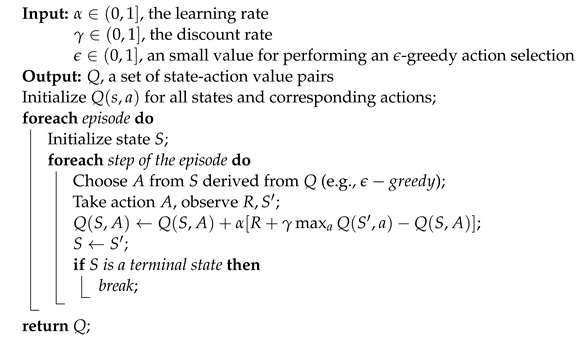
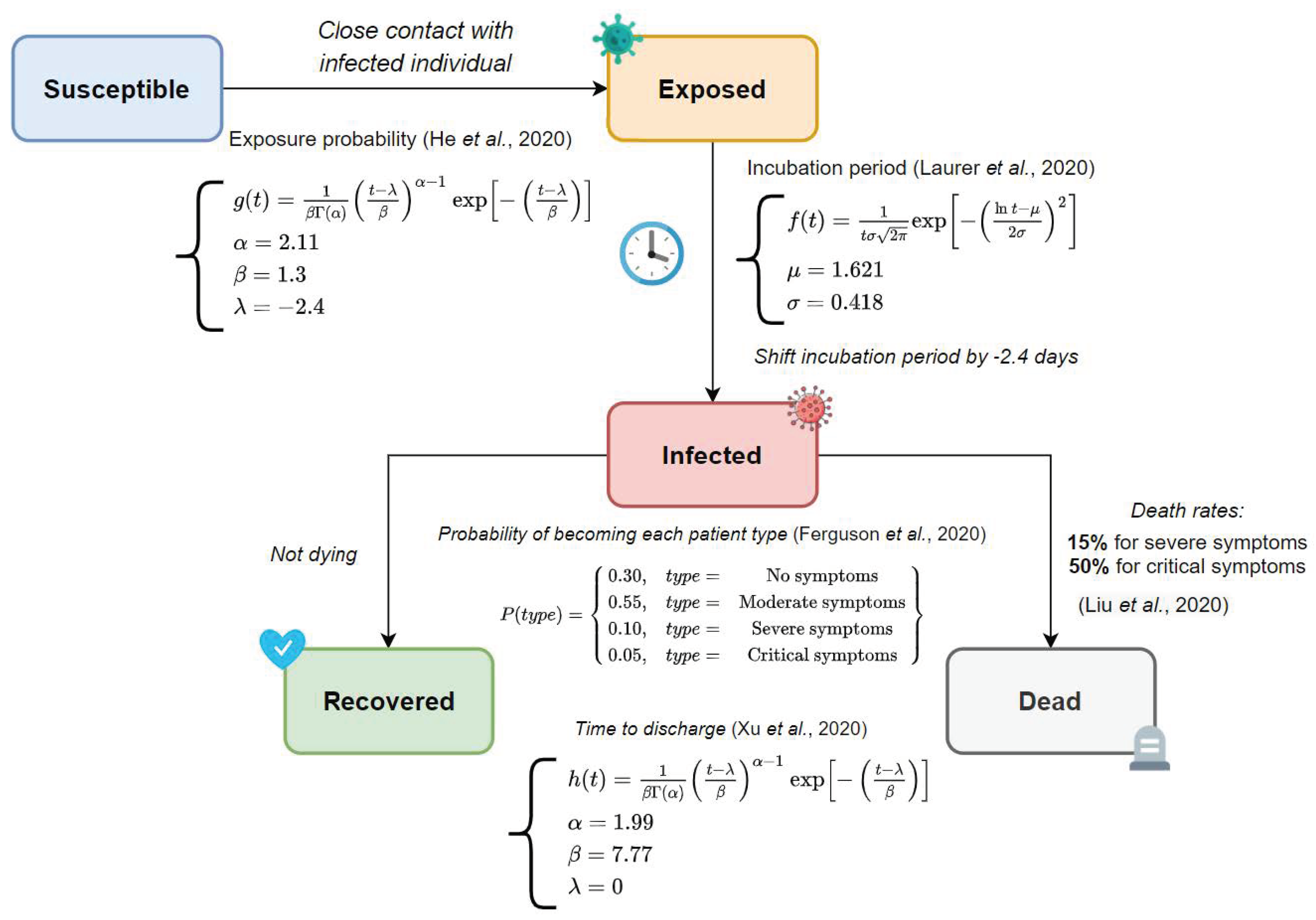
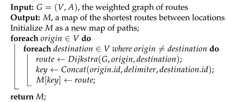
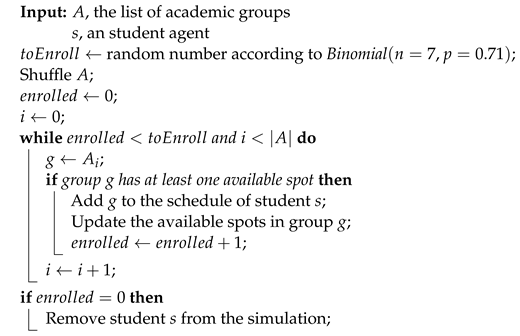
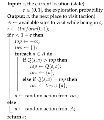
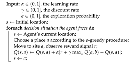
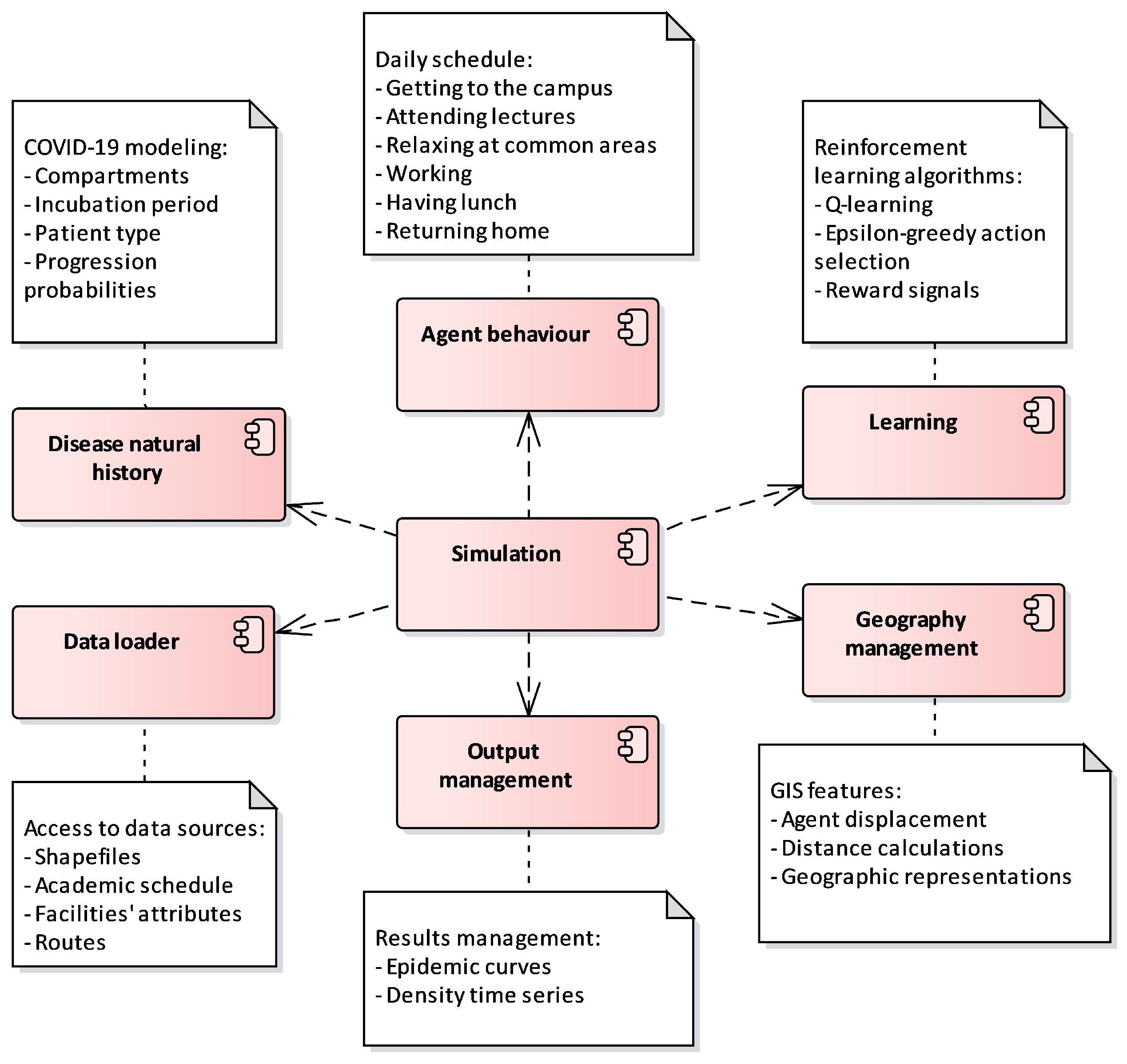


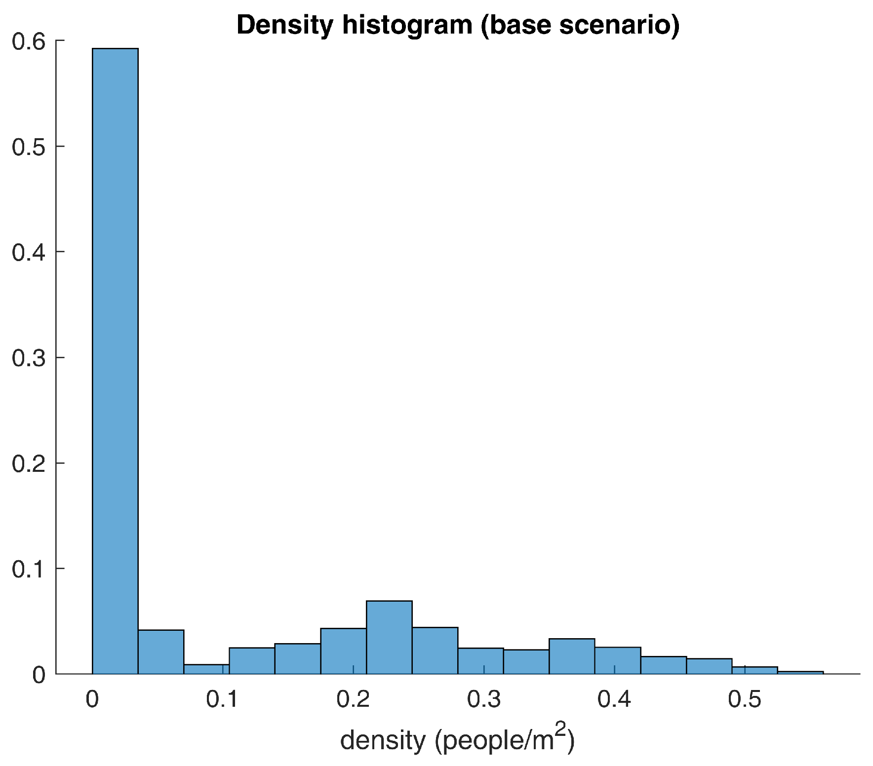
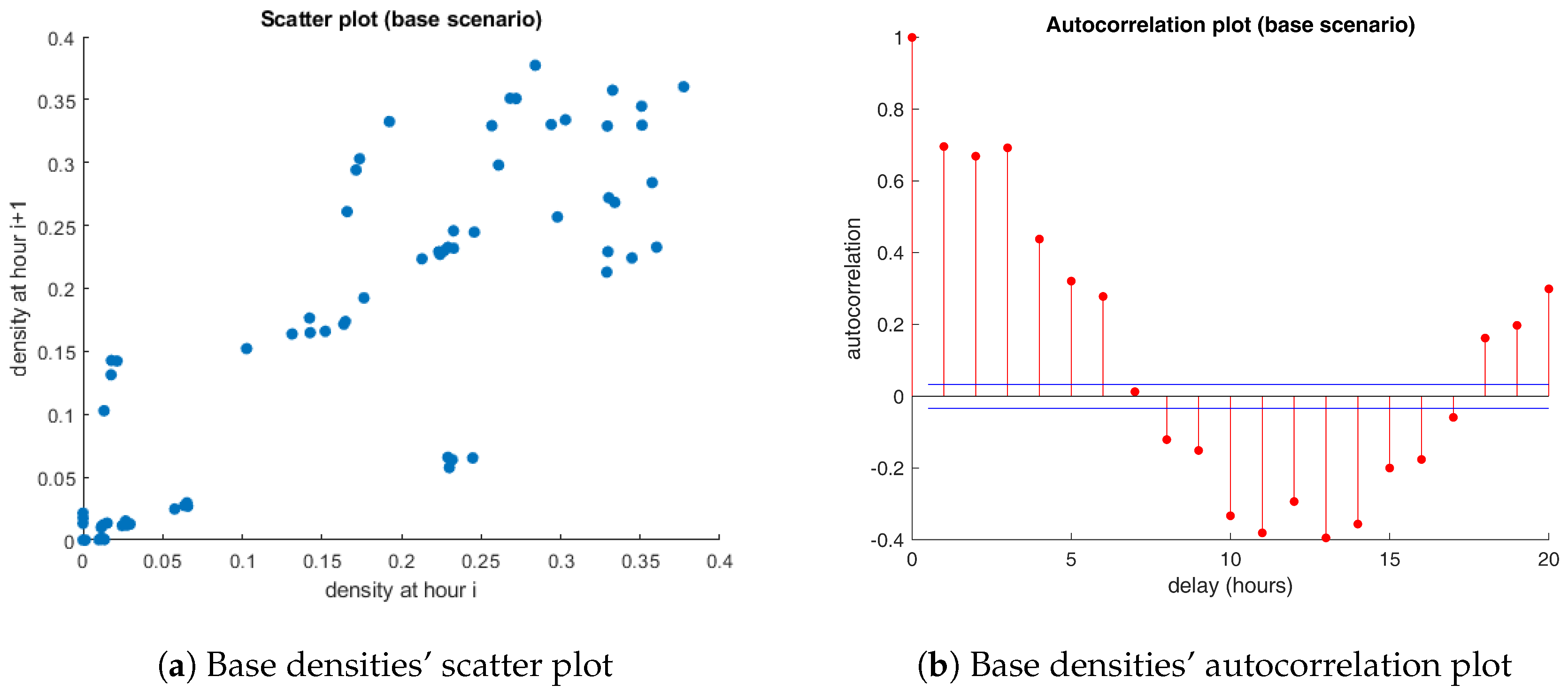
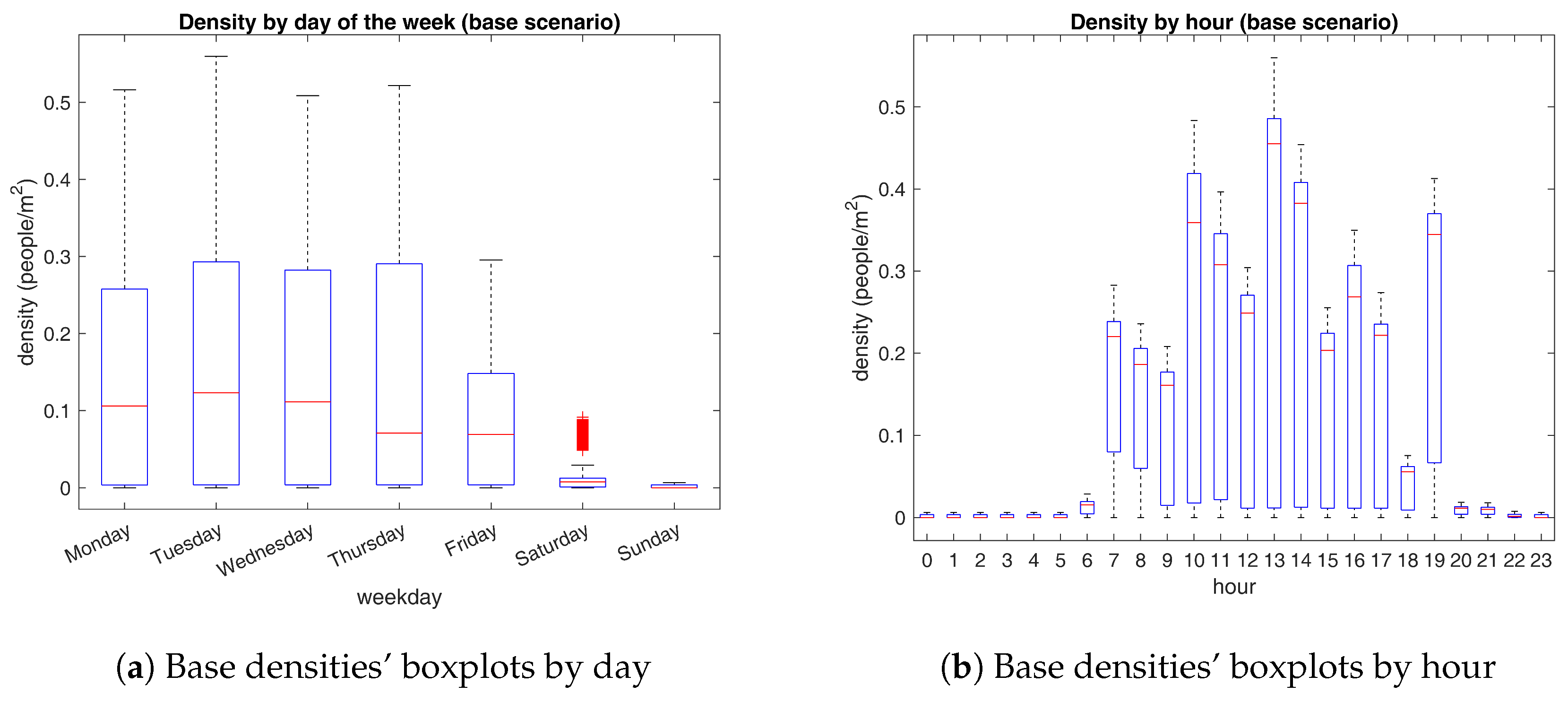
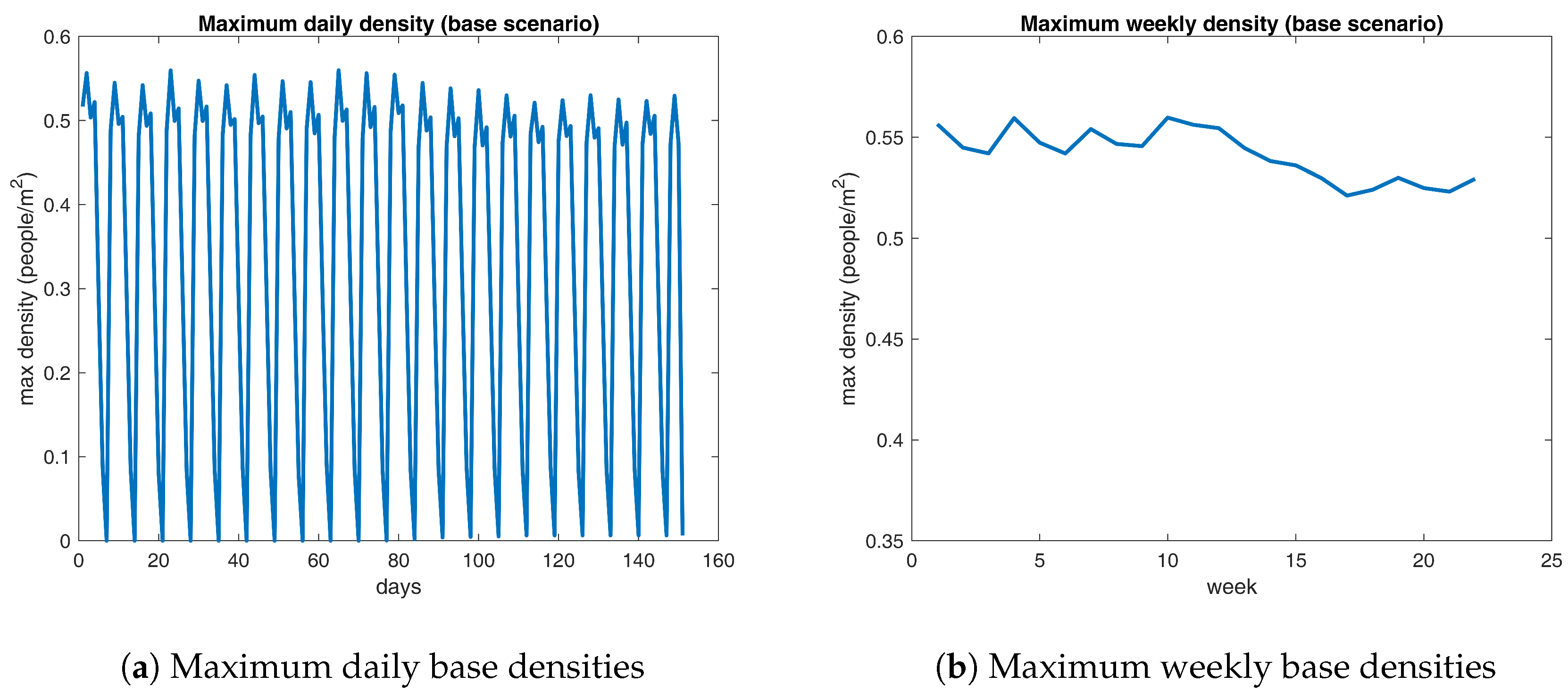
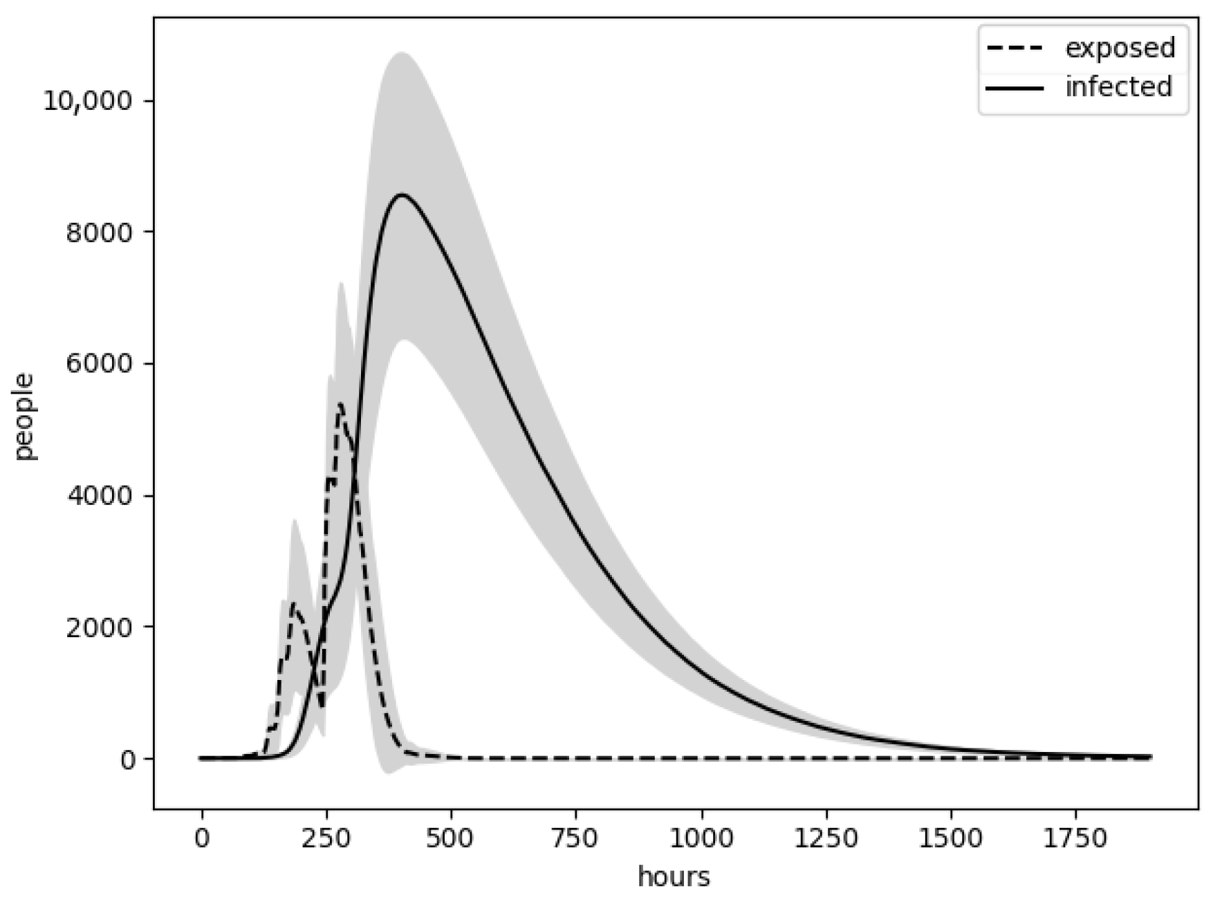

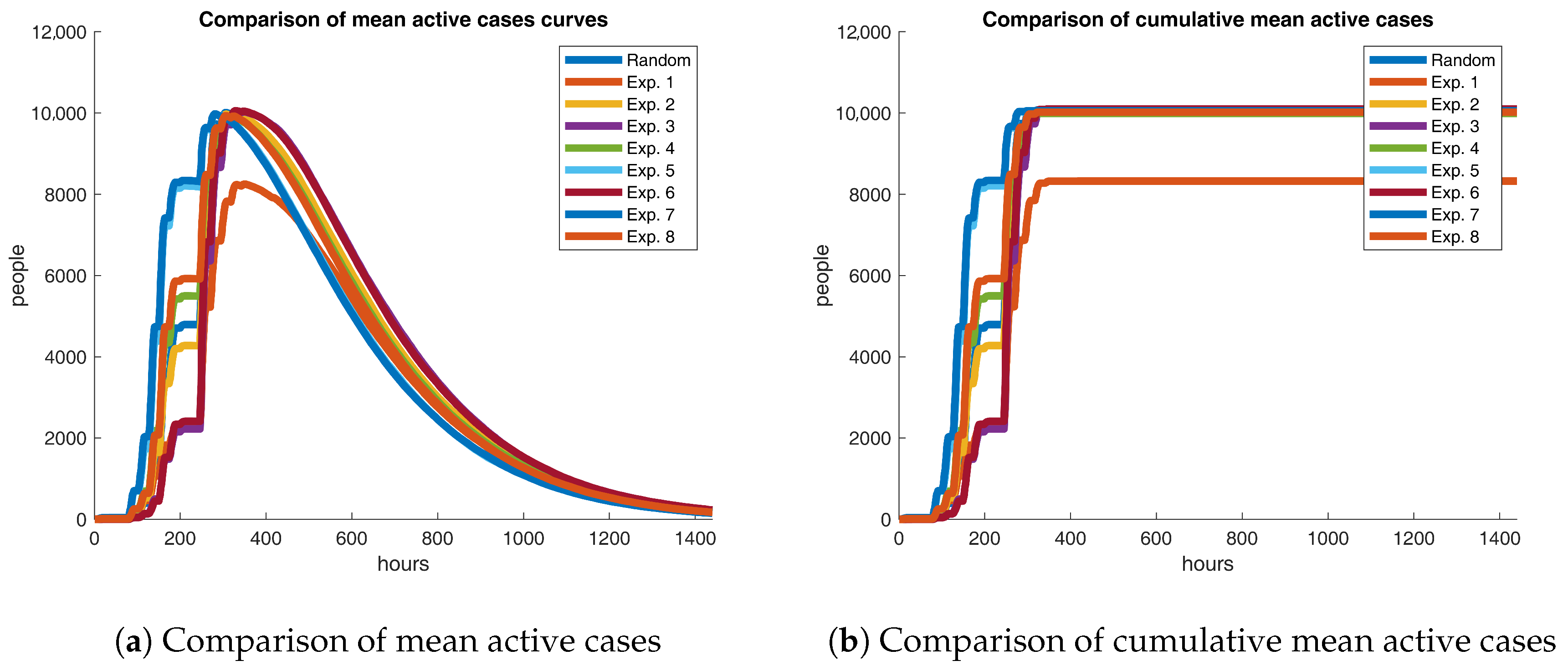

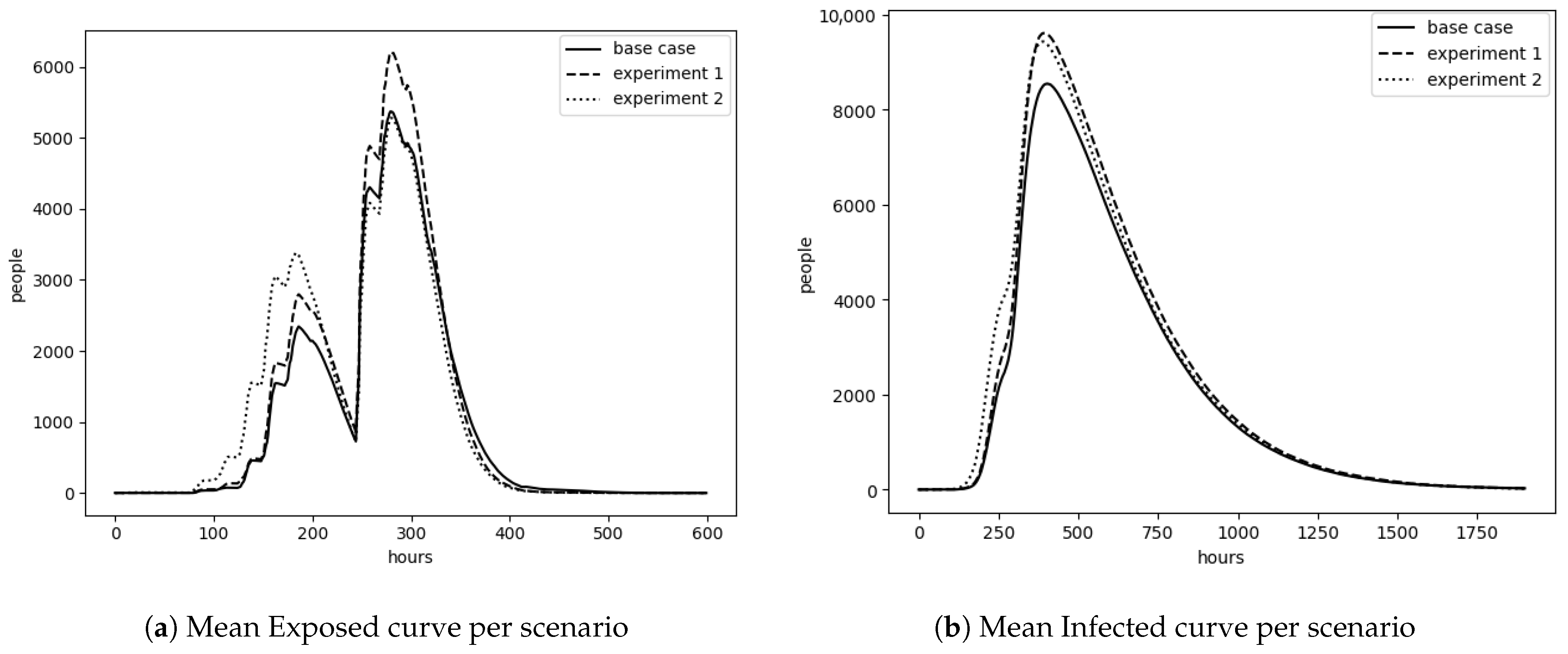

