Numerical Investigations and Artificial Neural Network-Based Performance Prediction of a Centrifugal Fan Having Innovative Hub Geometry Designs

Abstract

It is a well-known fact that air approaches the eye region of the rotating impeller of a centrifugal fan with shock-less entry conditions in an ideal scenario. The flow in this region is associated with induced swirl losses, leading to cumulative performance losses. Proper flow guidance in the vicinity of the eye region is essential to minimize possible flow losses. The flow guiding structure may be in the form of a projection or extrusion connected to the rotating impeller of the turbo machines and is generally named a hub. These attachments enhance the overall flow augmentation of the turbo machines in terms of static pressure improvement by reducing a significant amount of inlet turning losses. This article attempts to highlight the efficacy of hubs of various shapes and sizes on the pressure rise of the centrifugal fan using Computational Fluid Dynamics (CFD). Simulation results revealed that the optimized hub configuration yields about an 8.4% higher head coefficient and 8.6% higher relative theoretical efficiency than that obtained for the hub-less base configuration. This improvement in these paraments therefore also commemorates the global progress in energy efficiency as per the UN’s Sustainable Development Goals, SDG 7 in particular. Simultaneously, in the Artificial Neural Network (ANN), a Multi-Layer Perceptron (MLP) model is used to forecast the performance of a centrifugal fan with an optimized hub design. The results predicted by the ANN model are found to be in close agreement with the optimized hub shape’s numerical results.

1. Introduction

A centrifugal impeller’s entrance region typically experiences substantial turbulence, significant spiral flow losses, and flow stalling at the shroud as a result of abrupt changes in the flow direction. These flow losses tend to disturb the flow pattern at the inlet region, thereby causing both energy loss and a substantial reduction in the performance parameters of the devices. CFD is capable of analyzing the inlet flow domain, and whole field-flow analysis can capture the flow-loss phenomena effectively. A CFD study of relevant geometric interventions in the centrifugal fan’s inlet flow route demonstrates the potential for improved fan performance. Various methods for increasing the energy efficiency of the fan system result in the achievement of the aim set by the UN’s Sustainable Development Goals (SDG) for 2030. Significant contributions are made by various researchers to augment the performance of the fan by streamlining the flow characteristics of the device, particularly in the vicinity of the inlet region.

Jae Hyuk Jung et al. [1] studied the effects of the axial flow fan’s entry hub length and corner shape on efficiency. The losses as well as the efficiency were evaluated by performance parameters, such as total pressure loss. SC/Tetra v12, a commercial and popular CFD solver, was used for analyzing the fluid flow. The results revealed that for a certain entry hub length, efficiency improves, and the authors stated that this gain is due to the interaction between the hub vortex and the blade. Using CFD calculations, Vagnoli et al. [2] deliberated the start of stall events in a radial compressor of the transonic type. In the presence of inlet flow disturbances, the bent pipe provided at the impeller’s inlet eye region was evaluated. The authors revealed that the inlet flow losses are minimized in the presence of inlet guide vanes and these vanes essentially suppress the inlet flow disturbances. Wang Y et al. [3] analyzed a 90-degree curved pipe numerically for the performance assessment of two different types of inlet ducts: a normal straight duct and a radially bent duct. Their studies concluded that the inlet flow distortions are significantly suppressed in the case of a straight duct due to flow acceleration.

Numerical research of centrifugal fans with diffuser and nozzle types of inlet arrangements was conducted by Gholamian M et al. [4]. The results of the investigation showed that the flow geometry of the impeller inlet has a significant impact on the inlet flow losses. The authors concluded that nozzles with smaller diameters enable the fan to recover static pressure more effectively. To find out the impact of bell mouth forms on blower output, Son P N et al. [5] carried out a CFD analysis on a centrifugal blower. Twelve numerical models were created parametrically, each with a distinct bell mouth radius and gap between the upper fan casing and the mouth of the bell. To examine the blower’s transient characteristics, the frozen rotor approach was selected. The well-known realizable k-$\epsilon$ turbulence model successfully captures the turbulence behavior. Results showed that the flow coefficient is greatly improved by the bell mouth geometry. Yang C et al. [6] performed numerical studies on a radial compressor with an intake bleed flow and discovered that the relative Mach number significantly decreases toward the blade tip’s leading edge. The authors found that the recirculation avoids the separation of flow on the suction side of the impeller blade. In a multi-stage compressor, Cai [7] conducted a comparison between stator and cantilever hub topologies and found that the cantilever hub arrangement somewhat improves performance. He reasoned that the improvement was possible because the revolving hub offsets the gradients of static pressure along the route, thereby reducing the secondary flow.

The performance characteristics of the centrifugal fan are generally obtained through a set of experimentations conducted on a well-equipped test rig and a set of calibrated measurement devices. Hence, there is a dire need for a simplified process to investigate the fan performance characteristics in which a series of experimental performance tests can be avoided. The fan manufacturers and application engineers therefore also have a keen interest in obtaining the performance of fans for various geometrical interventions and multiple input conditions within the minimum amount of time. The requirement of the industry can be satisfied either by conducting the experimentation or by performing numerical analyses using built-in algorithms of fluid-flow analysis software. The task of numerical analysis is also found to be a challenging task due to the complexity of the geometrical configurations of the fan and additional computational requirements.

Alternatively, the fan’s performance characteristics may be predicted using an Artificial Neural Network (ANN). In this method, the pre-existing results procured from either experimentation or numerical work are used to obtain the desired fan characteristics. Nowadays, ANN is generally used in diversified domains such as solar heating, IC engines, control systems, biomedical analysis, forecasting, optimization, manufacturing, etc. Rajiv Tiwari et al. [8] performed experimentation on a centrifugal pump to study the severity of flow blockages and cavitation. The suction area restricted the flow of water into the impeller to achieve various levels of blockages. The rotational speed of the impeller was also varied to analyze the performance under various operating conditions. Pressure signals were captured using calibrated pressure transducers for various levels of blockages. The binary data classification method of deep learning was used to categorize the data obtained from pressure transducers. The authors found that the index of overall evaluation for the prediction accuracy is 98.32% for the combination of blockage and cavitation. Xu Ping et al. [9] predicted the adiabatic efficiency of the N-staged centrifugal pump based on an artificial intelligence technique and improved the prediction ability of the model using an S-fold cross-validation algorithm and smoothing factor circulation screening. They achieved a relative error in the range of 0.85–3.99%. Jie Pei et al. [10] verified the performance of a radial pump using multilayer ANN. Around 200 data sets obtained from numerical simulation were considered as the sample size for the ANN prediction. Particle swarm analysis was also incorporated into their prediction analysis. They achieved a marginal difference in pump efficiency of about 0.454% between CFD simulation and predicted value. A CFD analysis was conducted by Fernandes et al. [11] to obtain the relative and absolute flow structure near the impeller–volute region of a centrifugal fan. The study found that the significant interactions within the centrifugal fan were mostly localized in the impeller channels near the tongue area. Marlène Sanjose et al. [12] created the requisite sound modulation by simulating tonal noise control with a spinning impediment placed on the fan bell mouth. They showed that shaping the fan hub prevents flow separation at the hub and increases fan performance.

Yang et al. [13] used a centrifugal compressor impeller in their case study, and the line shape of the hub was changed to investigate the effect of line curvature on compressor performance. The numerical research findings revealed that within the design value range, the curvature of the impeller hub profile increased as the flow range and surge margin of the compressor impeller increased. Kuang et al. [14] discovered that the hub inclination angle (HIA) has a substantial impact on the flow characteristics of a centrifugal pump impeller. The large eddy simulation turbulence model is used in their research to simulate centrifugal pump impeller internal flow at two HIA values under design and off-design situations. The findings revealed that increasing HIA had a favorable influence on the head of the centrifugal pump impeller, with a 5% relative divergence between HIA values of 0° and 40°. Sagar et al. [15] studied centrifugal compressors with Bezier curved shroud profiles and circular arc contoured hub profiles. They discovered that the increase in surge margin is related to a shift in the blade angle at the inducer area, as the blade angle varies from hub to shroud at the blade’s leading edge.

According to the literature review indicated above, hub treatment in a centrifugal fan’s whole field-flow analysis has not yet garnered significant attention. The hub might improve airflow efficiency, boosting the fan’s total performance. The application of artificial intelligence for performance prediction in turbomachinery devices is therefore also limited. To close the gap described above, this article gives a numerical evaluation of the influence of different hub shapes on the overall performance of a centrifugal fan. Additionally, it explores the viability of appropriate design modifications for the hub’s size and shape. Secondly, by using a limited number of the numerical data sets, a multilayered neural network built in MATLAB is used to predict the performance of the centrifugal fan with minimum computational time. Finally, the ANN-predicted values are compared to the CFD findings.

2. CFD Modelling

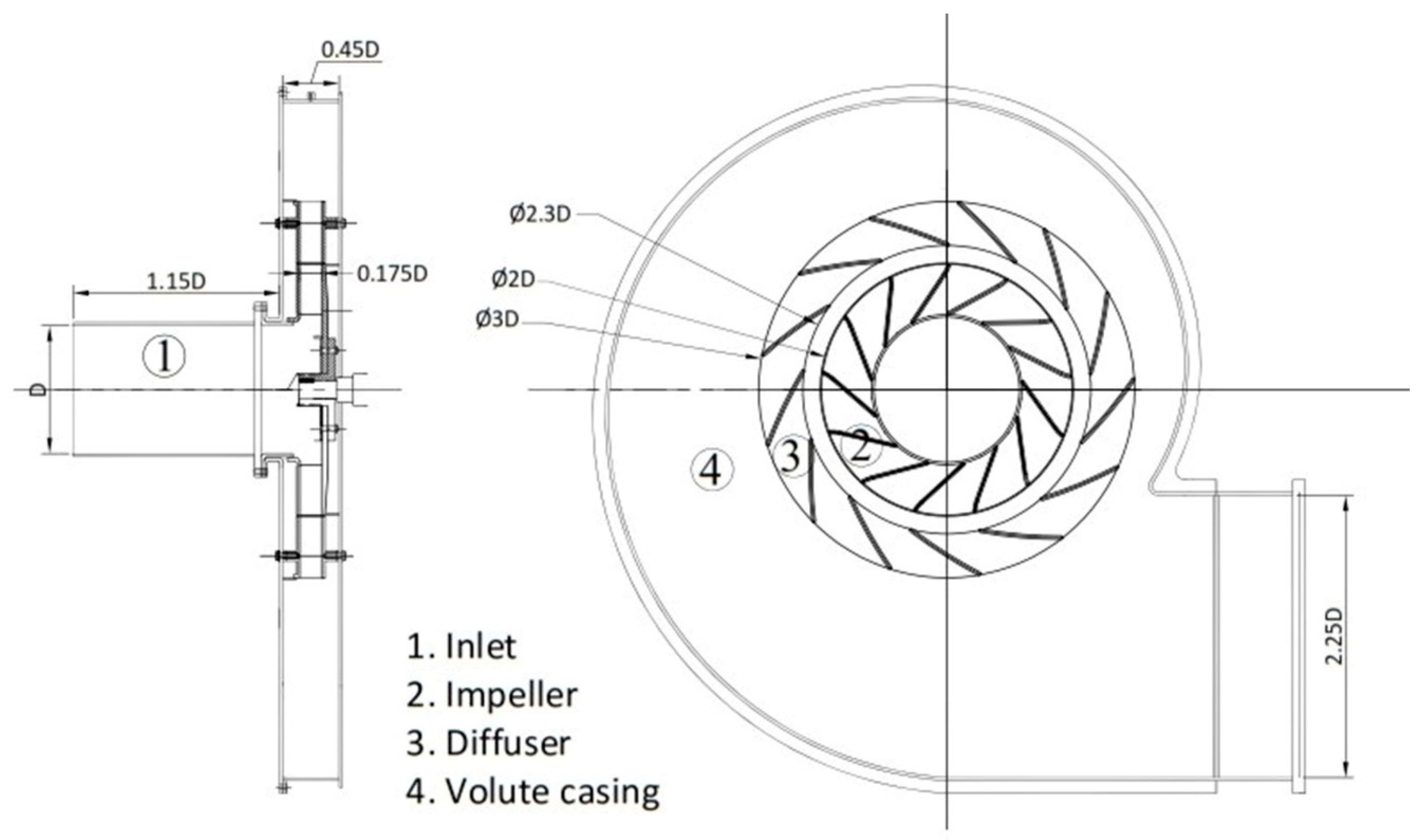
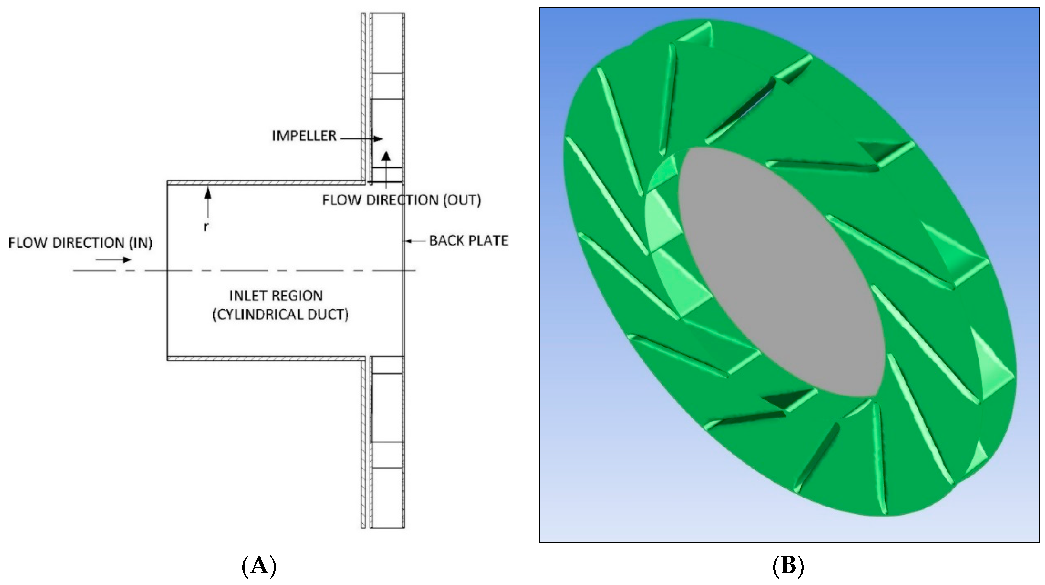
2.1. Geometrical Specifics

Figure 1 depicts the centrifugal fan employed in this investigation. This device’s cylinder-shaped inlet, backward-curved impeller, diffuser, and rectangular volute casing represent four essential flow domains. The technical publications by Meakhail and Park [16] and Madhwesh et al. [17] served as the foundation for the geometry of this test rig. In this study, this configuration is known as the hub-less base configuration.

The fan inlet is cylindrical and has a radius of 200 mm. An entrance length of about 1.15D is specified to ensure conformity in the flow characteristics at the impeller inlet and the entry region of the inlet pipe.

Table 1. Geometric specifications of the hub-less base model.

Impeller:
Radius at the inlet	: 0.6 D
Radius at the exit	: D
Inlet blade angle	: 30°
Exit blade angle	: 76°
Number of blades	: 13
Diffuser:
Diameter of the inlet	: 2.3 D
Diameter of the exit	: 3 D
Blade angle at the inlet	: 23 deg
Blade angle at the outlet	: 38 deg
Number of diffuser vanes	: 13
Volute casing:
Height of the channel	: 0.45 D
Flange width	: 2.25 D
Blade thickness	: 0.025 D
Impeller and diffuser passage width	: 0.175 D
The meridional gap between the diffuser and impeller	: 0.15 D
Rated RPM of the fan	: 1500

displays the fan’s geometric parameters.

2.2. Mesh Creation and Sensitivity Testing

According to the CFD code utilized in the current study, the mesh motion approach is applied for the transient analysis of the fan. Unstructured mesh domains, which are connected yet have overlapping interface zones, are needed for this technique. A mesh sensitivity study is conducted to check that the number of control cells utilized to mesh the fluid zone does not affect the numerical results. The mesh is initially created using large-sized element lengths equivalent to 42.3 lakh control cells, with the flexibility for localized smoothing for regions with high gradients, such as the border layer, wherever applicable in the zone. Regional mesh refinement is used to iteratively enhance the mesh with a steady decrease in cell element lengths to build finely meshed regions that correspond to 99.9 lakh cells. It can be demonstrated that there is almost convergence for the mesh density trials for the 68.9 and 99.9 lakh control volume cells. As a result, a mesh size of 68.9 lakh control volume cells was chosen for further numerical analysis [17]. This ensures that the memory storage and computation time required for the analysis are kept to a minimum. The distribution of the total control volume cells from the aforementioned investigation among the flow domains is shown in

Table 2. Control volume cell distribution in the flow area.

Zones	Inlet	Impeller	Diffuser	Volute Casing
Total number of control cells (in lakh)	13.6	13.8	21.7	19.8

.

2.3. Numerical Model Boundary Conditions

In the cylindrical coordinate of reference, the well-benchmarked CFD algorithm for moving mesh zones is used to solve the conservation differential equations for continuity, momentum, and scalar transport [18,19]. The numerical analysis’s boundary conditions closely match those in the author’s relevant experimental data [16]. This would result in a numerically accurate simulation. The no-slip assumption imposes a wall boundary limitation on the domain’s boundary surfaces, like the diffuser and impeller blades, as well as the inner portion of the volute casing. It is anticipated that the flow is completely established at the fan outlet, and Neumann boundary conditions are applied along the path of flow [16]. As recommended by Meakhail et al. [16], the intensity of turbulence is set at 5% in the turbulence model to simulate the turbulent flow behavior. The average hydraulic diameter required for the investigation is estimated in proportion to the inlet diameter of the fan [20]. A first set of 100 steady flow iterations is undertaken in the current study to establish dependent flow variables over the full domain for the time-periodic transient nature of the analysis that follows.

In the flow domains of centrifugal fans, fluid is frequently quite turbulent, having significant flow eddies and recirculation. Therefore, it is necessary to conduct a whole-field CFD analysis to capture the static pressure at several important parts of the flow domain and represent transient flow instabilities as time periodic fluctuations. Transient analysis is carried out using a pressure-based solver in conjunction with a second-order implicit velocity formulation [17]. Velocity, as well as pressure values, are coupled through the Patankar SIMPLE algorithm found in the CFD package. The second-order accurate upwind technique controls the discretization process. The turbulence model used in the analysis is the k-$\epsilon$ model available in ANSYS Fluent [16]. Mesh motion technology is used between the stationary diffuser and the rotating impeller, as well as between the rotating impeller and the stationary inlet region, with a time step of 0.1111 ms corresponding to the relative revolution of one degree. This condition will virtually satisfy the calculation scheme’s stability condition at a fan’s rated speed of 1500 rpm [17].

All of the residuals are given a pre-determined limiting value of 0.0001 as the first prerequisite for convergence. The moving mesh analysis is conducted iteratively twenty times for each stage. The weighted average values of velocity and pressure recorded at significant sites in the flow zone are acquired by conforming to one degree of revolution of the impeller using the time-step progression setup for the study.

2.4. Overview of the Output Parameters Used in the CFD Study

Hub effectiveness (${\epsilon }_h$), a non-dimensional variable, is defined as the ratio of total pressure loss for the model equipped with the hub to that for the model without a hub geometry. This is regarded as a local parameter that manages the pressure loss due to stagnation between the impeller’s input and outlet. It is defined by Equation (1).

$${\epsilon }_h=\frac{{\left(p_{t2}-p_{t1}\right)}_{with hub}}{{\left(p_{t2}-p_{t1}\right)}_{without hub}}$$

(1)

The static pressure rise coefficient ($\zeta$) and the total pressure-loss coefficient ($\omega$) are two global metrics that are defined to represent the centrifugal fan’s overall performance. Equations (2) and (3), respectively, define them.

$$\zeta =\frac{1}{N}{\displaystyle \sum _{j=1}^{j=N}\left(\frac{p_4-p_2}{p_{t2}-p_2},t_{initial}+j\Delta t\right)}$$

(2)

$$\omega =\frac{1}{N}{\displaystyle \sum _{j=1}^{j=N}\left(\frac{p_{t2}-p_{t4}}{p_{t2}-p_2},t_{initial}+j\Delta t\right)}$$

(3)

where $p=\frac{1}{N}{\displaystyle \sum _{j=1}^{j=N}p(node of area,j)}$.

The following equations, Equations (4) and (5), are used to derive the performance variables, volume and head coefficients, respectively.

$$\varphi = \left(\frac{Q}{\pi R_o^2 U_2}\right)$$

(4)

$$\psi = \left(\frac{p_3}{\rho U_2^2}\right)$$

(5)

Furthermore, the relative theoretical efficiency is described as the ratio of transferred energy gained from CFD analysis to that obtained from Euler’s equation. It is defined in Equation (6).

$${\eta }_{Rt} = \left(\frac{H_{CFD}}{H_{th}}\right)$$

(6)

2.5. Validation of the Numerical Analysis

The base model without a hub is numerically simulated to derive the head as well as volume coefficients stated in the numerical analysis. The numerical formulation for the validation research employs identical input parameters as the experimental work. Figure 2 and Figure 3, respectively, [14] exhibit the characteristic curves for head vs. volume coefficient and relative theoretical efficiency versus volume coefficient for experimental and numerical data.

The differences between the CFD and experimental outcomes in terms of error percentage are computed. The 3σ confidence bound for the difference between CFD and experimental values for the head coefficient ranges from 2.41% to 6.36%, while the 3σ confidence bound for the error between experimental and CFD values ranges from 2.15% to 9.83% for relative theoretical efficiency.

According to the 3σ confidence limits, 99.7% of the experimental values are consistent with the CFD results. The experimental findings and 3σ confidence limit for errors are in quite good agreement with the numerical outputs for the main characteristic plot and operating characteristic graph. The confidence bounds logically illustrate that the numerical analysis findings are compatible with the experimental data, with negligible nonconformities reflecting losses due to leakage and other flow-loss effects.

2.6. Different Hub Geometries Used in the Numerical Analysis

As seen in Figure 4A,B, in the vicinity of the impeller eye region, the flow in a standard hub-less base design abruptly switches from axial to radial.

The main goal of the current analysis is to reduce the areas of stalling inceptions close to the impeller’s inlet region. This is achieved by offering hub designs that are either hemispherical or elliptical, as depicted in Figure 5 and Figure 6, respectively. To investigate the effectiveness of the hub in each scenario compared to the hub-less base configuration, numerical calculations are carried out separately for hemispherical (Figure 5A) and ellipsoidal (Figure 6A) designed hubs. The equivalent numerical models of the inlet region with a hub are shown in Figure 5B and Figure 6B. To enable the hub’s rotation with respect to the impeller, CFD software (2021 version) provides it with a “moving wall boundary condition”.

The geometry employed for the variation of ellipsoidal hub configurations is the length of the hub in the axial direction, whereas for hemispherical hub configuration it is the hub radius. For the hemispherical and ellipsoidal hub models, these two parameters are non-dimensional in terms of the entrance radius of the duct and are known as the spheroidal hub ratio and the ellipsoidal hub ratio, respectively.

$$\mathrm{Spheroidal} \mathrm{hub} \mathrm{ratio}, R_s=\frac{r_h}{r}$$

(7)

$$\mathrm{Ellipsoidal} \mathrm{hub} \mathrm{ratio}, R_E=\frac{l_h}{r}$$

(8)

In the analysis, the parametrically changed values of the spheroidal hub ratio and ellipsoidal hub ratio are listed in

Table 3. Ellipsoidal and spheroidal hub ratios used for CFD analysis.

Hemispherical Hub		Ellipsoidal Hub
Model	Spheroidal Hub Ratio	Model	Ellipsoidal Hub Ratio
Hub-less base	0.00	Hub-less base	0.00
S1	0.30	E1	0.30
S2	0.40	E2	0.50
S3	0.50	E3	0.70
S4	0.60	E4	0.90
S5	0.70	E5	1.10
S6	0.80	E6	1.30

. The hemispherical hub geometry’s radius is optimized to produce the ellipsoidal hub’s meridian height (d), as further discussed in Section 3.1.

3. Results and Discussion

3.1. CFD Analysis

The effectiveness of the hub (${\epsilon }_h$) is used to compare several parametrically variable hub configurations against the hub-less base model to meaningfully show the influence of hub shape on flow characteristics.

Additionally, two overall output parameters are used: the static pressure increase coefficient and the total pressure-loss coefficient. These parameters support the hub’s effectiveness in terms of total enhancement in static pressure increase across the fan. These calculated parameters correspond to volume coefficients between 0.004 and 0.051. Various histograms are used to display the changes in these important parameters due to various hub geometry configurations. To better understand flow physics in combination with performance characteristics, velocity contour graphs are created. The effectiveness of the modified hub on performance is explored to use the fan at its design point. The effectiveness of the hub with off-design flow conditions is then discussed.

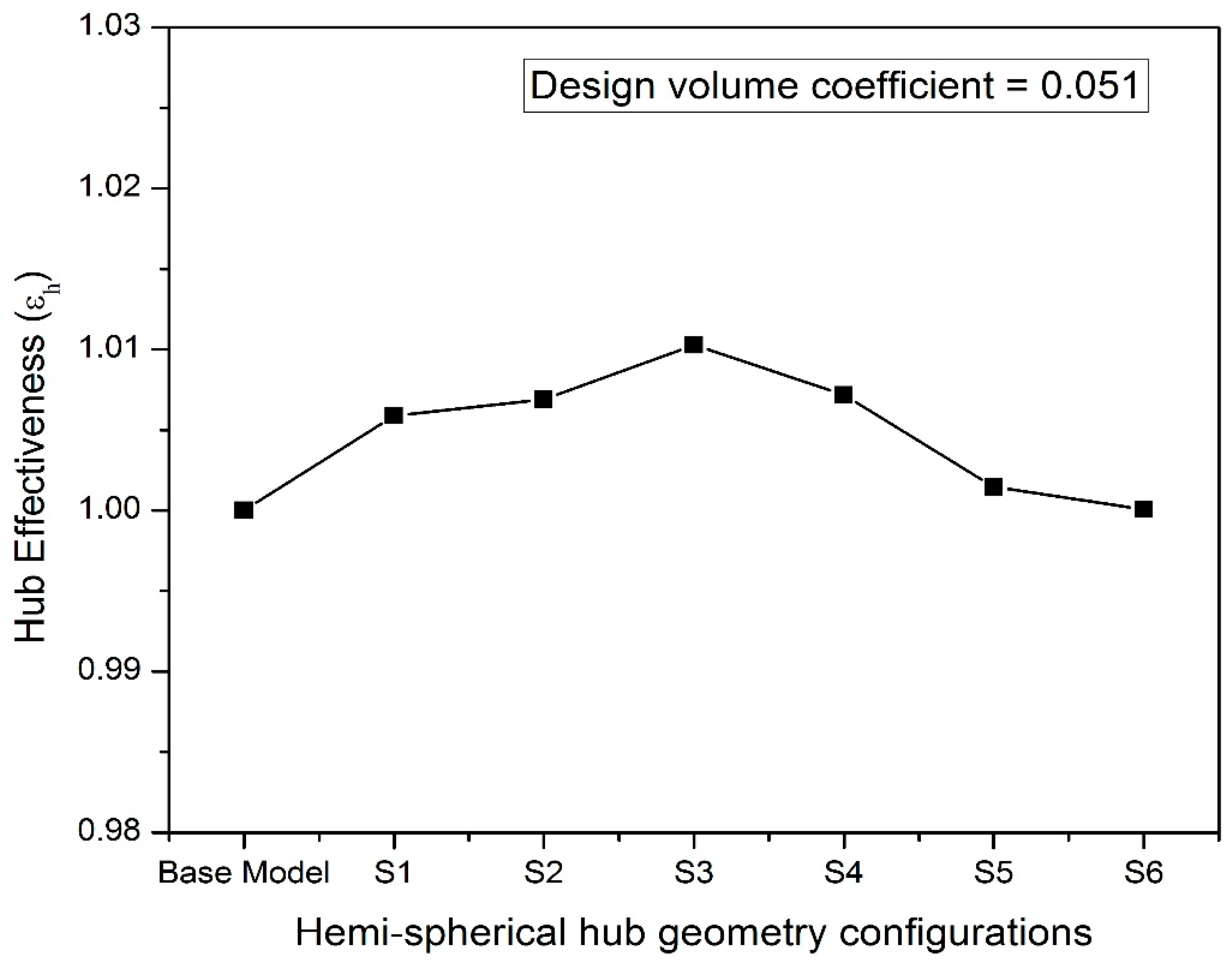
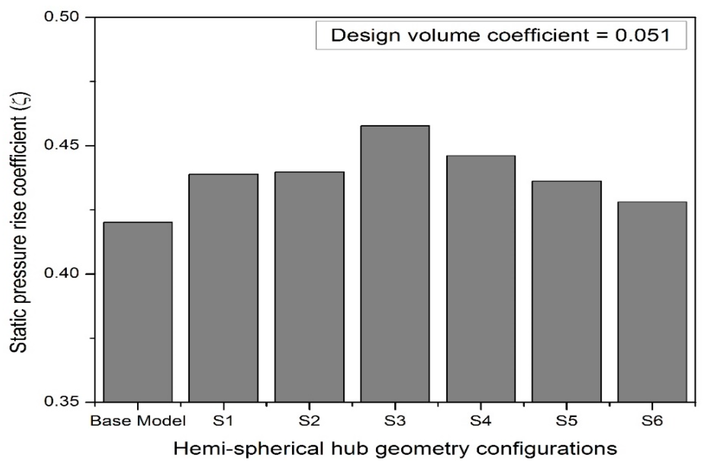
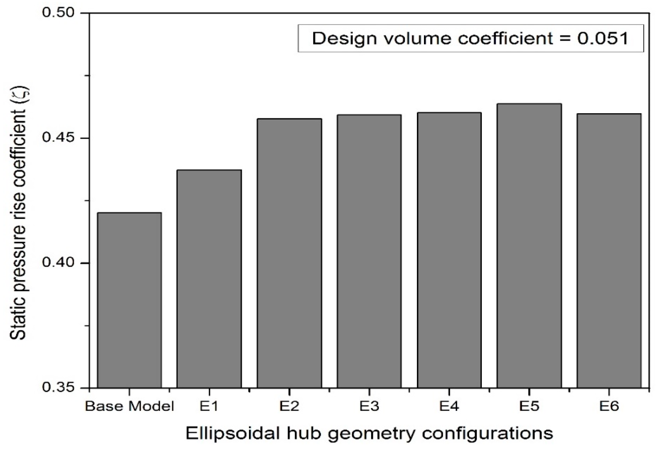
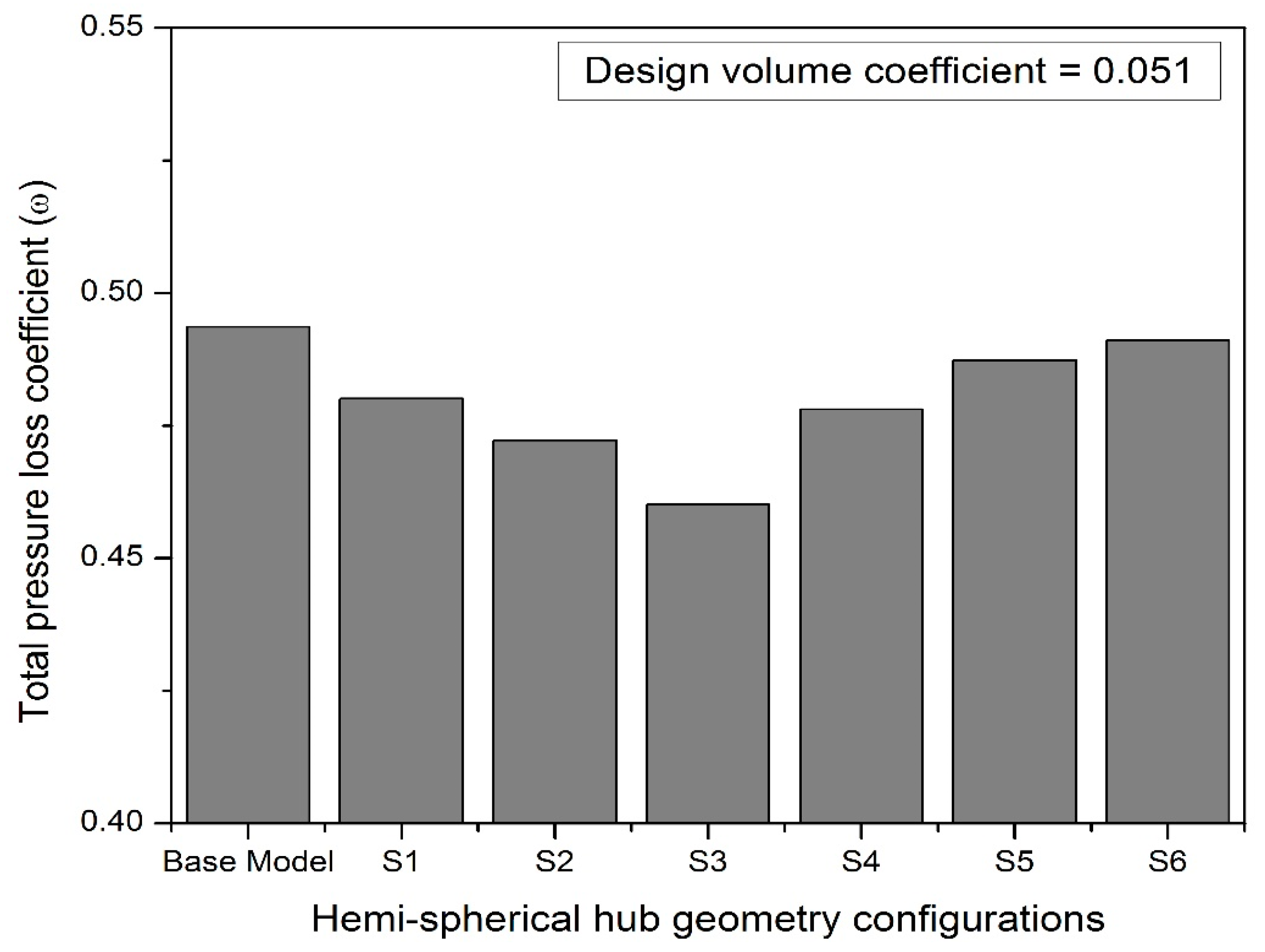
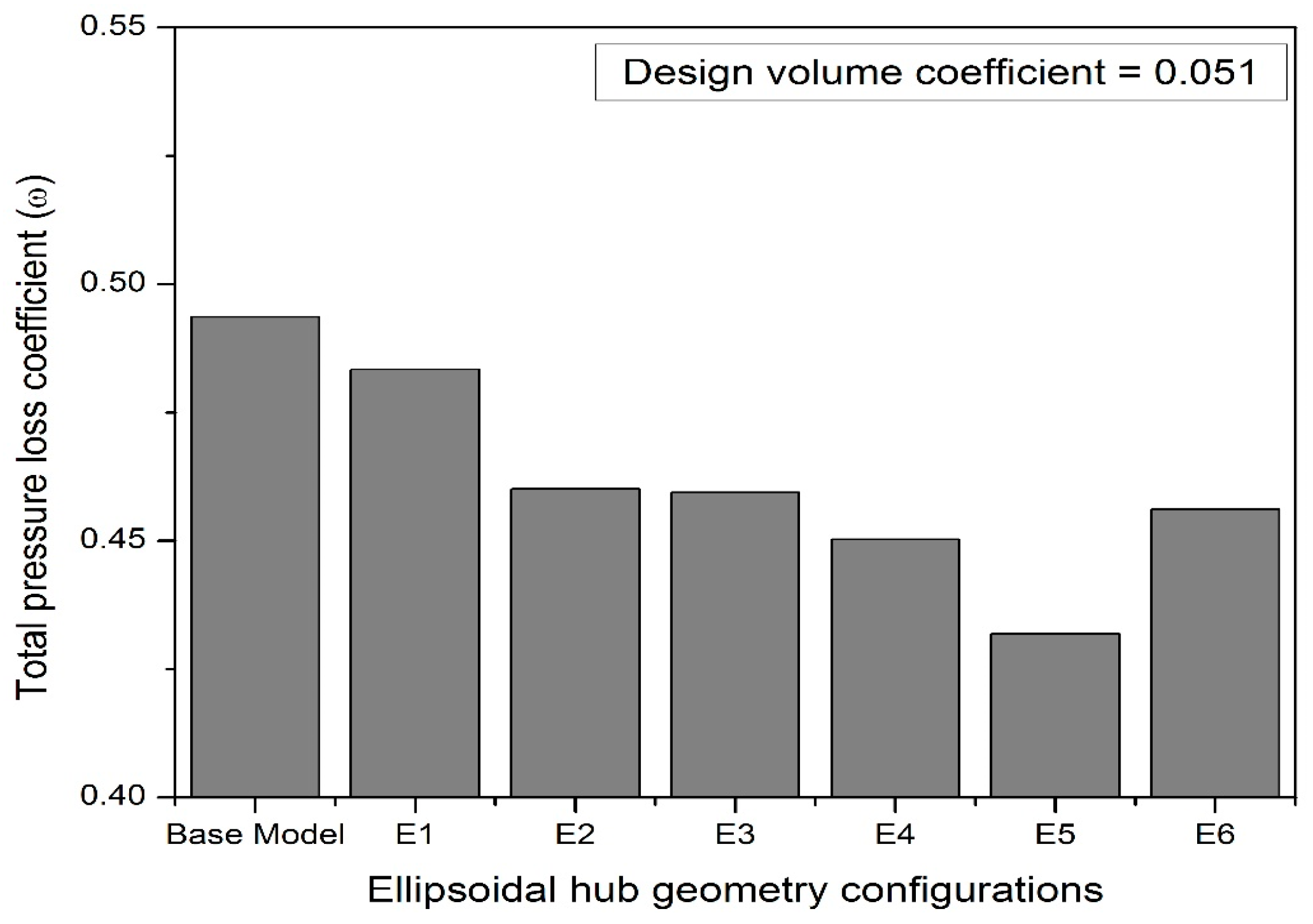
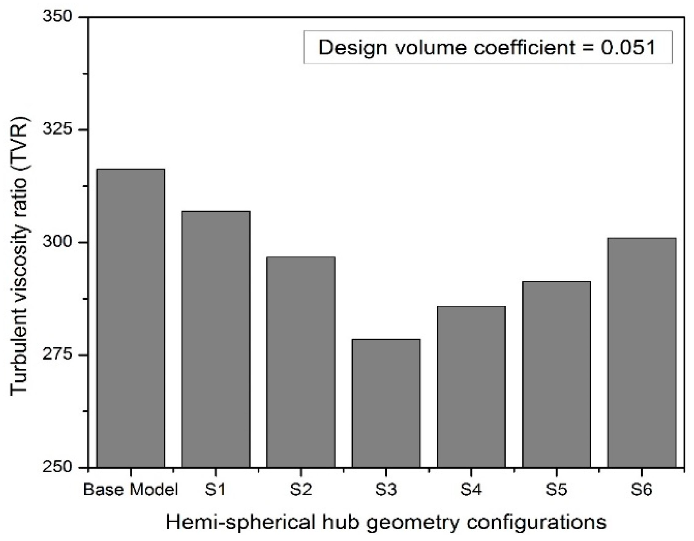
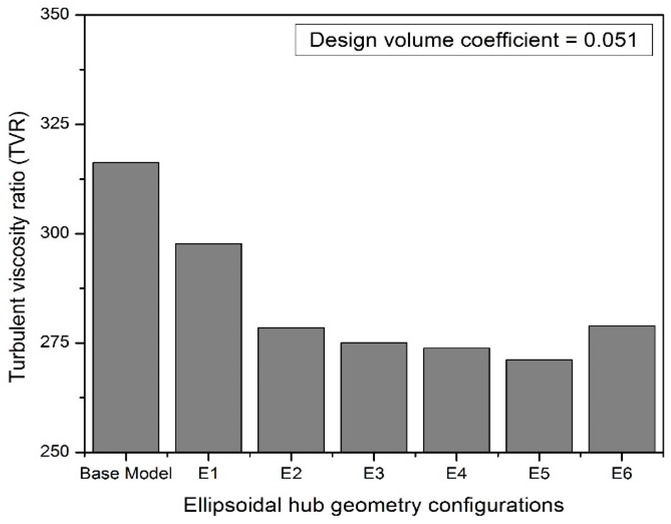
3.1.1. Performance Augmentation of the Fan Due to Hub Geometry Treatment at Design Mass Flow Rate

As demonstrated in Figure 7A,B, air tends to experience a stalling effect on the back-side shroud plate while moving along the suction tube. It depicts the type of flow at the fan’s inlet eye area for the hub-less base model. It has been revealed that the presence of low-pressure stall disturbances causes a significantly disturbed flow field of velocity when fluid enters the rotating impeller. A proper geometric intervention in the eye region is required to decrease this. Hub designs with spheroidal and ellipsoidal hub ratios varying from 0.30 to 0.80 and 0.30 to 1.30, respectively, are investigated to establish the optimal hub model geometry that will result in minimum flow distortions at the fan inlet and finally re-align it with the main stream.

Figure 8 and Figure 9 show the trend of the effectiveness of the hub for various hemispherical and ellipsoidal hub geometry configurations at the design point volume coefficient of 0.051. The research reveals that, compared to the hub-less base model, improved hub effectiveness is attained for all the configurations of hemispherical and ellipsoidal hub geometries. For configurations S3 and E5, respectively, a hub effectiveness improvement of 1% and 1.7% above the hub-less basic model is noted.

This is explained by the fact that the hub’s hemispherical or ellipsoidal shape eliminates the stalling effect seen in the hub-less base model and improves flow direction into the impeller’s meridian inlet route. Here, it must be emphasized that the main causes of flow losses are stalling at the hub wall and turbulent flow at the impeller’s entrance brought on by the swirling of incoming fluid. This can be explained by stating that for these configurations, the flow losses brought on by turbulence are decreased, improving the fan’s overall performance.

Additionally, it appears that hub effectiveness is at its highest for configurations S3 (corresponding to a spheroidal hub ratio of 0.5) and E5 (corresponding to an ellipsoidal hub ratio of 1.1). This is attributed to the fact that for configurations S3 and E5, in addition to the streamlined through flow that was previously described, useful acceleration was also attained, which tends to flush the swirling eddies, thereby efficiently guiding the flow. Because of this, it can be seen that these geometric configurations, as depicted in Figure 10A and Figure 10B, respectively, significantly lower flow-related losses, particularly stalling losses, in the vicinity of the impeller’s inlet when compared to the hub-less base model. Therefore, it is clear that among the combinations examined for higher static pressure recovery, these geometric configurations appear to be the best hub designs.

Contrarily, it can be seen from Figure 8 that the hub effectiveness significantly decreases for hemispherical hub topologies with spheroidal hub ratios higher than 0.50. As shown in Figure 9, the useful hub effectiveness of ellipsoidal hub configurations likewise exhibits a decreasing trend for hub ratios above 1.10.

One of the potential causes could be that as the hub ratio is raised, the through flow is choked off as air passes through a smaller path near the impeller’s eye, as depicted in Figure 11A and Figure 11B, respectively. Due to the “jet effect”, which is characterized by velocity cubed losses, this results in a substantially higher turbulent jet flow entering the impeller, which significantly lowers the fan performance.

Two performance variables—static pressure rise coefficient and total pressure-loss coefficient—are also employed to assess the hub treatment outcomes. The static pressure rise coefficient variation for various hemispherical and ellipsoidal hub geometry configurations is shown in Figure 12 and Figure 13, respectively. Regardless of the hub shape, it appears that all the hub geometry combinations employed in the current analysis efficiently control the flow and lessen the previously described inlet distortions. In comparison to the hub-less base structure, these configurations have a comparatively higher static pressure-rise coefficient due to the enhanced flow condition that arises, which also contributes to decreased inlet flow losses. Additionally, the effect of diminishing the inlet disturbances is expressed as a decrease in the total pressure-loss coefficient, as seen in Figure 14 and Figure 15 for hemispherical and ellipsoidal hub configuration geometries, respectively.

Additionally, the variation in the values of the turbulent viscosity ratio is depicted in Figure 16 and Figure 17 for various hemispherical and ellipsoidal hub geometry configurations investigated during the analysis. As shown in Figure 16, for hemispherical hub geometry configurations, the turbulent viscosity ratio decreases up to the spheroidal hub ratio of 0.5. According to Figure 17, the turbulent viscosity ratio decreases up to an ellipsoidal hub ratio of 1.1 for ellipsoidal hub geometry configurations. The outcome is an improvement in static pressure rise performance for all the hub geometry combinations.

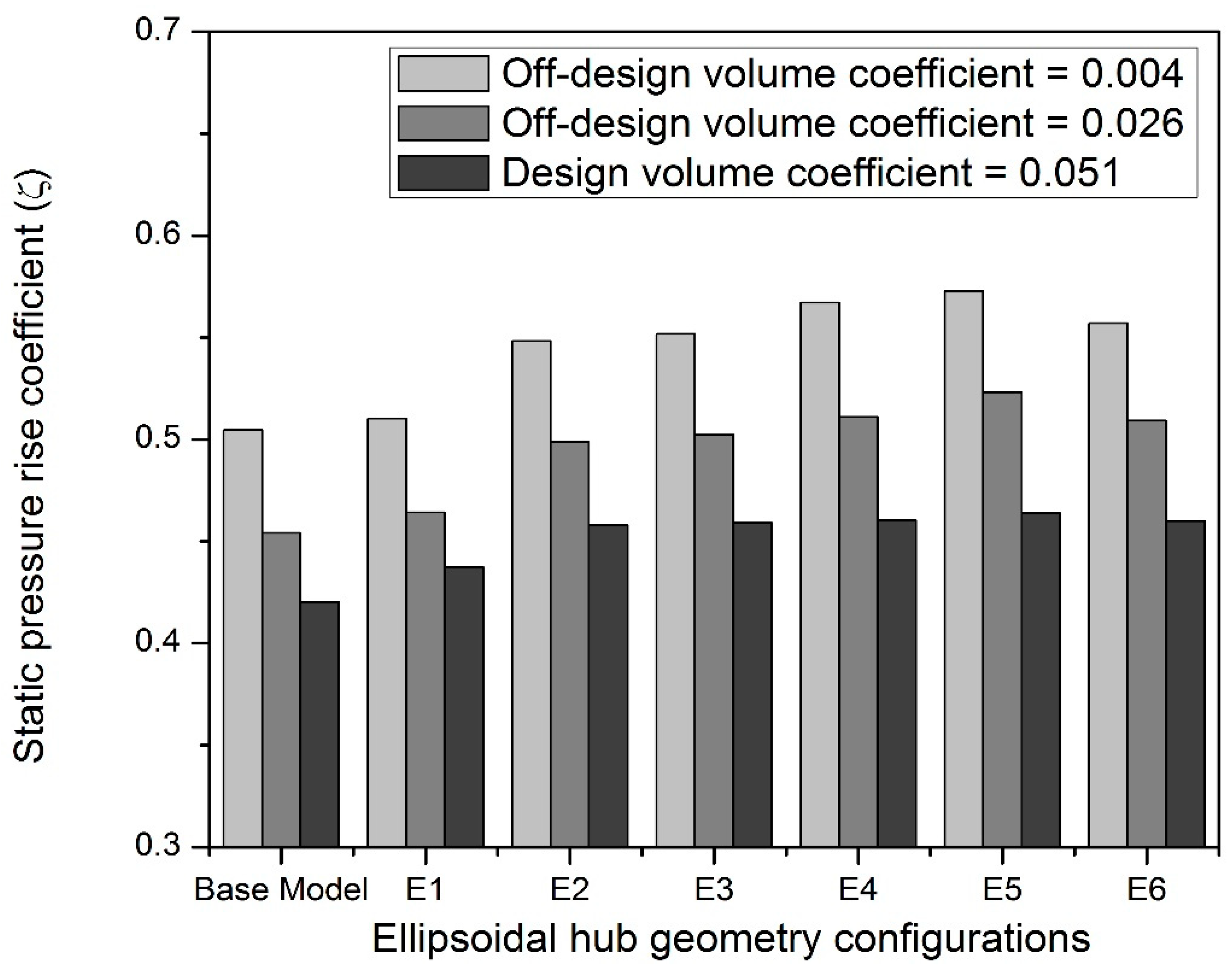
3.1.2. Effect of Hub Geometry Treatment on Performance for Off-Design Conditions

The effect of hub configuration is assessed for the design volume coefficient of 0.051 and the optimum hub geometry configuration is identified as described in the previous section. Encouraged by the results obtained for the designed volume coefficient, the effect of off-design volume coefficients on the performance indicators relating to the various hub geometry configurations is also studied numerically. The volume coefficients considered in the analysis have values between 0.004 and 0.051. The static pressure rise coefficient constantly declines as the volume coefficient increases, as shown in Figure 18 and Figure 19. This holds for both the hemispherical and elliptical hub shape combinations used in the study as well as hub-less base configurations.

The hemispherical hub configuration S3 and the ellipsoidal hub configuration E5 are found to be the best design configurations, offering comparatively higher static pressure rise coefficients for any of the volume coefficients used in the analysis, when compared to other configurations, which also include the hub-less base model. In comparison with the hub-less base configuration model, the enhanced hemispherical hub geometry configuration S3 exhibits a significant increase in the static pressure-rise coefficient of around 3.27%, and the optimized ellipsoidal hub geometry E5 exhibits an improvement in the static pressure-rise coefficient of about 6.07%. Therefore, it can be deduced that for increased fan performance, it is beneficial to opt for either a hemispherical hub geometry that corresponds to a spheroidal hub ratio of 0.50, or an ellipsoidal hub geometry that corresponds to an ellipsoidal hub ratio of 1.10.

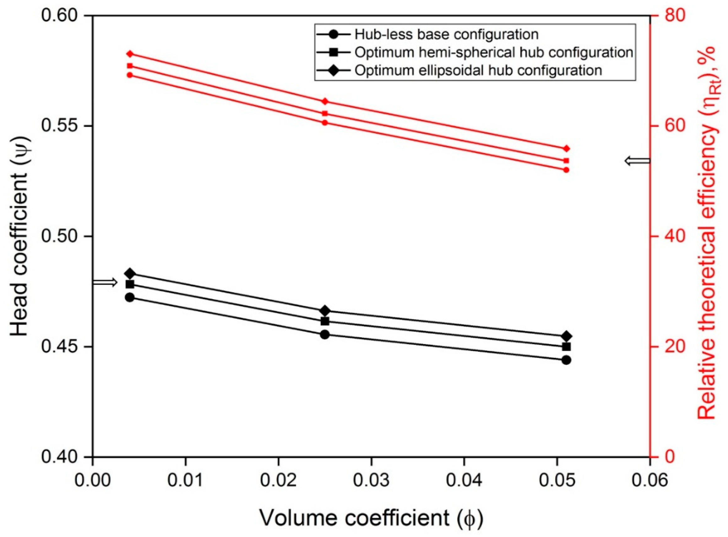
3.1.3. Optimal Hemispherical and Ellipsoidal Hub Arrangement Comparison

The goal of the current study on optimum hub geometric designs involved hubs of both the hemispherical and ellipsoidal types. The comparative analysis of fan performance for several ideal hub geometry combinations is covered in this section. Head coefficient and relative theoretical efficiency were used as the performance metrics for this investigation.

The optimal hemispherical hub configuration (S3) and elliptical hub configuration (E5) are shown in Figure 20 in comparison to the hub-less base configuration. It can be shown that the best ellipsoidal design (E5) slightly improves the head coefficient for all volume coefficients adopted for the present study. On average, this configuration results in a better head coefficient, i.e., 8.4% higher than that of the hub-less base model, while the same configuration produces a considerable increase in the head coefficient of roughly 1.04% above the hemispherical hub model (S3).

Similar to this, Figure 20 shows the relative theoretical efficiency plot for the best elliptical hub (E5) and hemispherical hub (S3) designs. It can be shown that for the optimal hub configurations, the relative theoretical efficiency trend of variation follows the head coefficient trend. It can be seen that, on average, the best hub geometry configuration (E5) delivers an 8.6% gain in relative theoretical efficiency over the hub-less base model and a 3.8% increase over the best hemispherical hub model for the range of volume coefficients taken into consideration (S3).

Both performance parameters seem to favor the ellipsoidal hub arrangement E5. This can be deduced from the fact that, when compared to a hemispherical hub model, the turning losses close to the impeller’s eye certainly decrease in the presence of an optimized ellipsoidal hub arrangement. As a result, the flow in the inlet region is being streamlined better, and the overall gain for the entire fan is an improvement in both the head coefficient and relative theoretical efficiency for the E5 design.

3.2. Artificial Neural Network Prediction Analysis

3.2.1. Background of ANN Model

ANN methodology is dependent on mathematical models that are programmed to execute various functions. It works along similar lines to the information processing of a human brain. Many neurons are connected to input and output layers. These neurons collect the information from the sources, perform non-linear operations and present the final value as output. The total number of input and output variables decides the number of neurons. For engineering problems, generally a feed-forward back-propagation model or multilayer perceptron model is used. It consists of an input layer, output layer and hidden layer. The input layer collects the data from the sources, whereas the output layer yields results. The general layout of the MLP model is shown in Figure 21. The input data and their associated interconnecting weights are provided for the summing junctions. As per Equation (9), the outcome of the summing junction along with the bias of neurons is fed to the transfer function to generate the final output.

$$u_j=F\left[\left({\displaystyle \sum _{i=1}^n{a}_i{w}_{ij}}\right)+b_j\right]$$

(9)

The selection of these functions is based on various parameters such as the complexity of the problem, biasing weights and node numbers. It is very much essential to have a proper relationship between input and output value, which ensures the realistic output value for a given input. The most common type of transfer function used in ANN is as given in Equation (10).

$$F(X)=\frac{1}{1+e^{-X}}$$

(10)

The input and output parameters used in the analyses generally have variations in terms of their range. To normalize the data and to convert them into a consistent range from –1 to +1, Equation (11) is used and is given by

$$Y=(Hig{h}_{value}-Lo{w}_{value})\frac{Y_i-Y_{\min }}{Y_{\max }-Y_{\min }}+Lo{w}_{value}$$

(11)

The various types of back-propagation algorithms widely used in ANN applications are Bayesian Regularization, Scaled Conjugate Gradient and Levenberg–Marquardt. Bayesian Regularization, generally referred to as TRAINBR, converts a non-linear regression problem into a statistical problem. The training with this method is more robust and gives good prediction accuracy. However, it takes higher training time. The scaled Conjugate Gradient method, known as TRAINSCG, requires derivative functions for input, weights and transfer functions. This method yields results with lesser accuracy, but it is possible to achieve lesser training time. Levenberg–Marquardt, popularly called TRAINLM, is a tradeoff method in which the Jacobian matrix and the gradient vector are calculated. TRAINLM requires relatively lesser training time with moderate prediction accuracy.

3.2.2. Proposed ANN Model

It is understood from CFD analyses that the performance indices of centrifugal fans are dependent on geometrical configurations as well as operating variables. The input factors influencing the performance are the ellipsoidal hub ratio (R_E) and volume coefficient ($\varphi$) for the optimized hub configuration, i.e., ellipsoidal hub model. The output parameters chosen for ANN studies are head coefficient ($\psi$) and relative theoretical efficiency (${\eta }_{Rt}$). The model has an input layer, output layer and hidden layer. The input layer consists of two neurons, representing the flow coefficient and ellipsoidal ratio for an ellipsoidal hub configuration. The output layer has two neurons for head coefficient and relative theoretical efficiency for the ellipsoidal hub configurations. The range used for input and output parameters is shown in

Table 4. Range of input and output parameters.

Parameters	Range
Input parameters
Volume coefficient	0.004–0.051
Ellipsoidal Ratio	0–1.3
Output parameters
Head Coefficient (Ellipsoidal)	0.4440–0.4898
Relative Theoretical Efficiency (Ellipsoidal) in percentage	52.79–71.65

. A schematic representation of the ANN model used for the prediction of the performance of the centrifugal fan is depicted in Figure 22.

3.2.3. Key Performance Indices for ANN Study

The performance prediction capability of the trained ANN network is assessed using the following parameters:

Correlation Coefficient (R): This number indicates the fitting of predicted data with the actual output data and it is given by Equation (12). Better performance of the ANN model is reflected in a value of R close to unity.

$$\mathrm{R}=\frac{{\displaystyle \sum _{i=1}^n\left(Y_{P,i}-{\overline{Y}}_P\right)\left(Y_{A,i}-{\overline{Y}}_A\right)}}{\sqrt{{\displaystyle \sum _{i=1}^n{\left(Y_{P,i}-{\overline{Y}}_P\right)}^2{\displaystyle \sum _{i=1}^n{\left(Y_{A,i}-{\overline{Y}}_A\right)}^2}}}}$$

(12)

Root Mean Square Error (RMSE): This is a measure of the standard deviation of actual results of CFD analysis from the ANN-predicted results and is given by Equation (13). It describes the spread of predicted results around the regression line. The accuracy of the predicted result is better if the value of RMSE is lower.

$$\mathrm{RMSE}=\sqrt{\frac{1}{n}{\displaystyle \sum _{i=1}^n{\left(Y_{A,i}-Y_{P,i}\right)}^2}}$$

(13)

3.2.4. ANN Model Training and Simulation

In the present ANN analysis, 35 sets of sample data are taken from the CFD analysis for ellipsoidal hub geometry configuration. Neural Network Analysis is carried out using MATLAB R2021b to predict the performance of the fan. To estimate the performance parameters of the centrifugal fan, the MLP model available in the software is used. The data set is shared for training, testing and validation in the ratio of 70:15:15 on a random basis.

Selection of Training Algorithm

The training is performed using three available training algorithms, namely Levenberg–Marquardt (TRAINLM), Scaled Conjugate Gradient (TRAINSCG) and Bayesian Regular (TRAINBR). The number of neurons in the hidden layer is arbitrarily chosen to be between three and eight in increments of one. This wide range of the number of neurons ensures that the RMSE attains a relatively lower value. The network is trained using all three algorithms for all the cases of the hidden layer. Figure 23 depicts the variation of RMSE for all the training algorithms used for the chosen number of neurons in the hidden layer.

It is seen from Figure 23 that RMSE is relatively minimal for the TRAINBR training algorithm irrespective of the number of neurons in the hidden layer. As mentioned earlier, due to the robust and accurate training performance, the error seems to be minimum for TRAINBR, and hence this algorithm is considered throughout the analysis for the prediction of results.

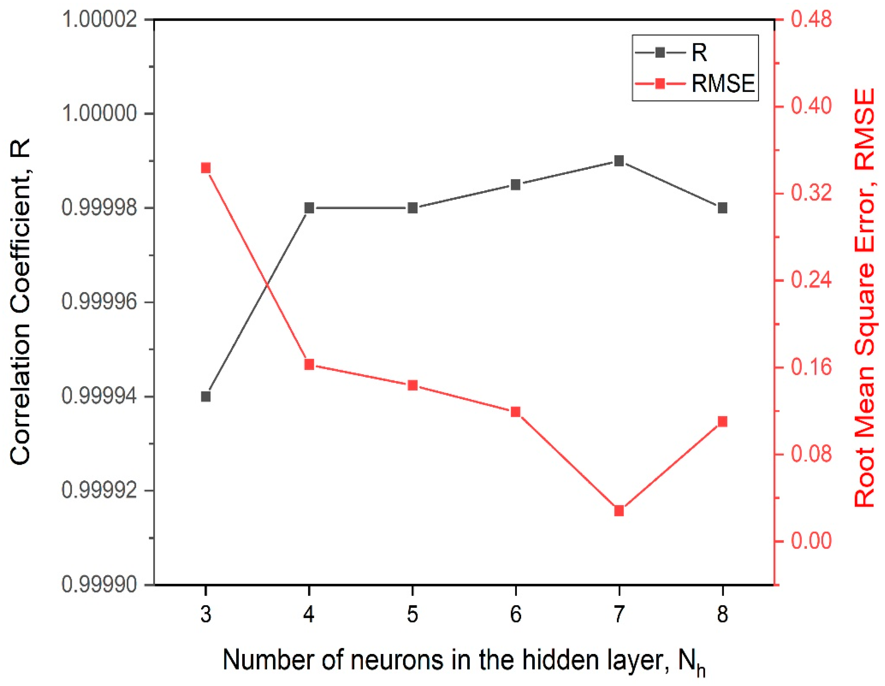
Selection of the Number of Neurons in the Hidden Layer

In an ANN analysis, the number of neurons in the hidden layers is identified based on the trial and error method. There is no clear expression readily available to determine the exact number of neurons to be considered in the hidden layer which would give the optimum performance. However, researchers in the past used many rules of thumb to determine the number of neurons in the hidden layer.

Harish et al. [21] reported a trial-and-error method of determining the number of neurons in the hidden layer with the help of Equation (14):

$$N_h=\left[0.5\times (I+O)\right]+\sqrt{T_R}$$

(14)

Using this relation for the present analysis, the total number of neurons in the hidden layer is found to be seven.

Also, to verify the above fact, the training is performed using TRAINBR as the training algorithm. The number of neurons in the hidden layer is varied from three to eight in increments of 1. For each case, the Correlation Coefficient (R) and Root Mean Square Error (RMSE) are captured, and the variations are depicted in Figure 24.

It is observed that the value of R is found to be 0.99999 and is the maximum for seven neurons in the hidden layer. For the same neuron number, RMSE is found to be 0.028 and is the minimum among all the other configurations of neurons in the hidden layer. Hence, in the present analysis, the hidden layer with seven neurons is considered. The 2–7–2 architecture of the neuron networks is displayed in Figure 25.

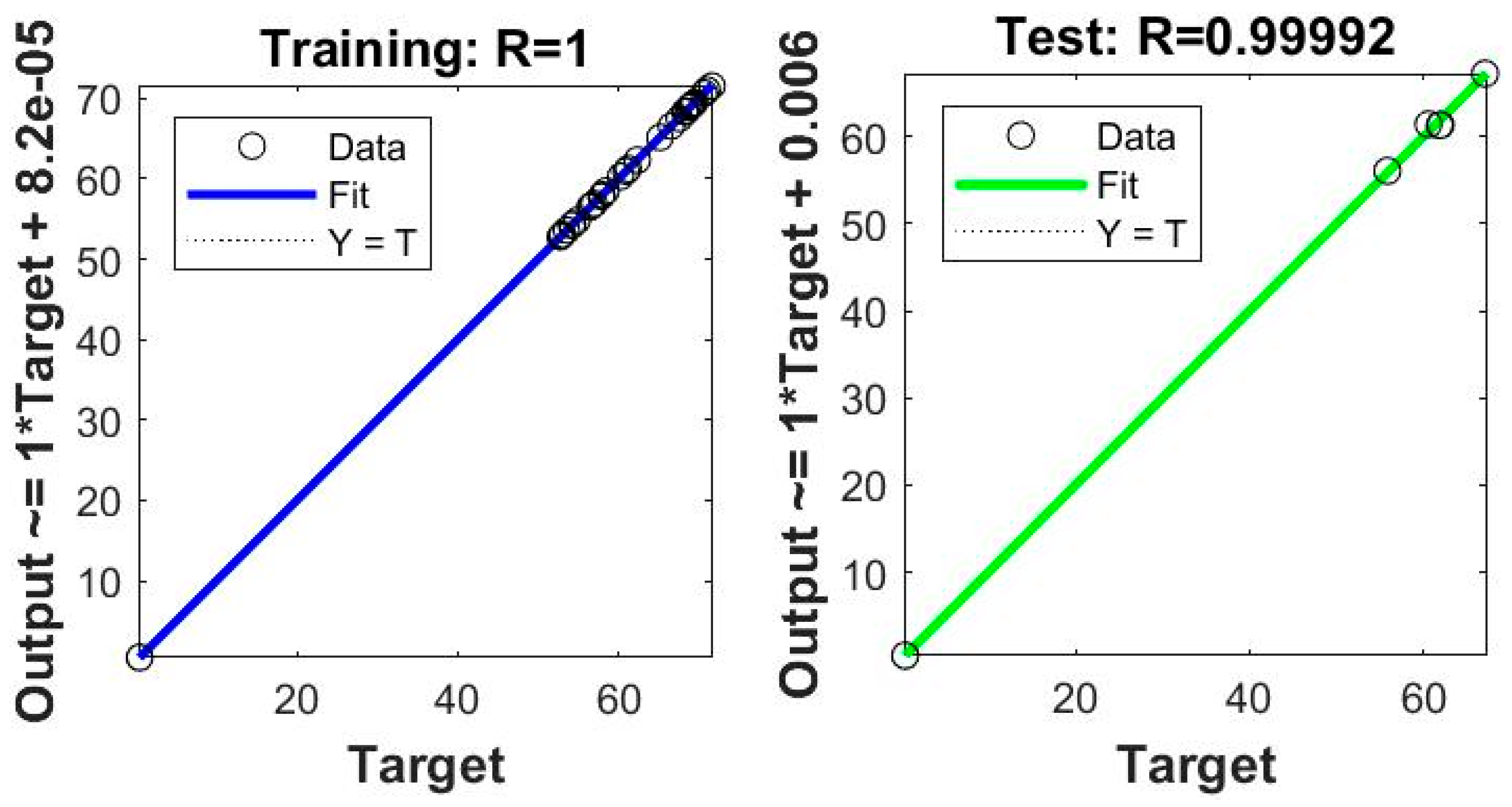
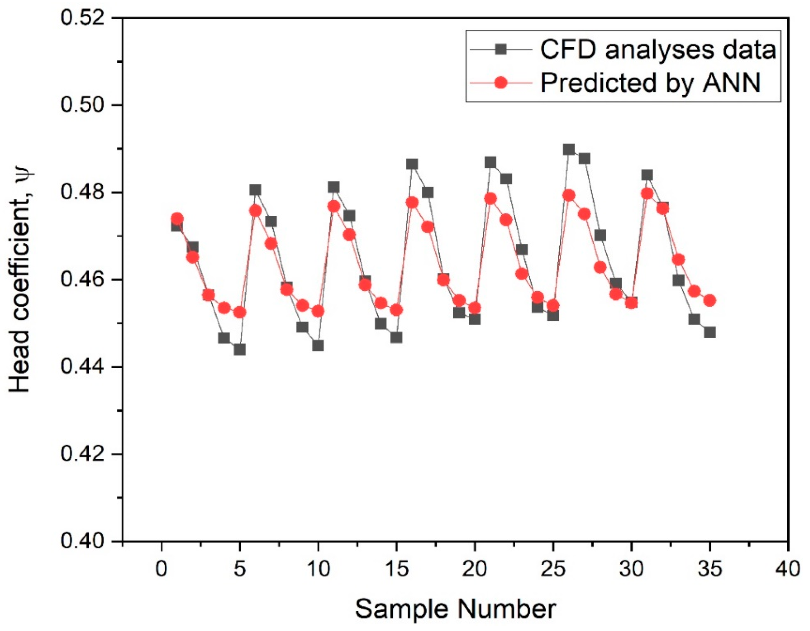
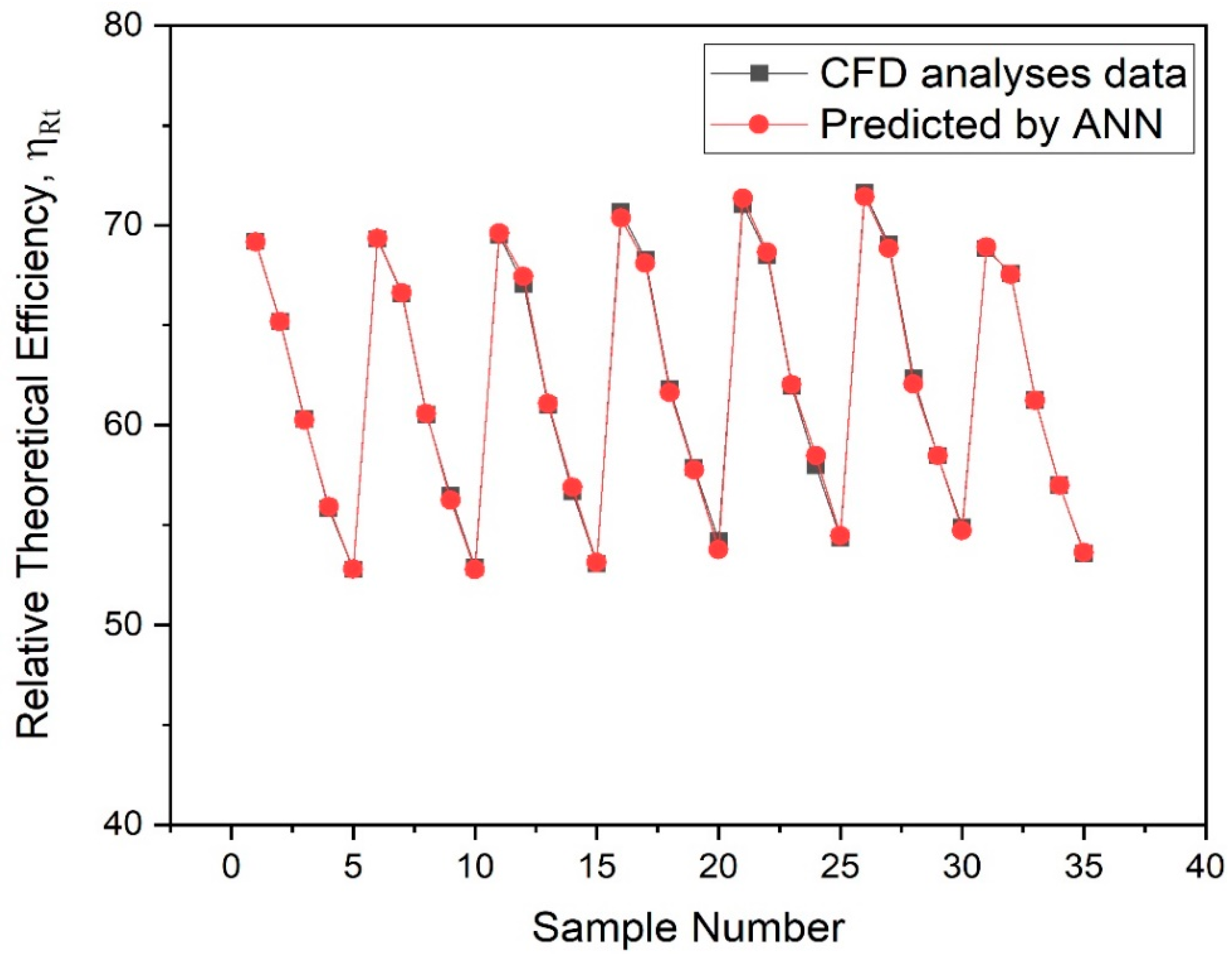
Results of the Training Process

Figure 26 depicts the regression graph plotted against the best-fit line. It is seen from this figure that the correlation coefficient values are 1.00000 for the training set, 0.99992 for the test data and 0.99999 for the overall data set used in the study. Also, the results predicted by the ANN training model will fit closely with the results obtained by the numerical analysis. Hence, it is concluded that the data obtained in the CFD analysis are precisely predicted by the chosen ANN model.

Figure 27 and Figure 28 depict the comparison of head coefficient and relative theoretical efficiency values obtained through CFD analyses and those predicted by ANN, respectively. It is seen that the highest error of 0.013 in head coefficient and 0.43% in relative theoretical efficiency is obtained. The values of average error for head coefficient and relative theoretical efficiency are found to be 0.0008 and 0.0002%, respectively, and are well within the range of acceptable limits.

The deviation between actual and predicted values is due to the generalized fitness of the network during the training process, i.e., during the learning process, if the noisy or fluctuating data are picked up by the model, then they will affect the developed model negatively. This results in the overfitting observed for some of the predicted values. Hence, it is concluded that ANN can be employed to predict the output parameters of a centrifugal fan equipped with an optimized hub using the limited number of CFD simulation results. Through this approach, a huge amount of manual effort, as well as a significant amount of time, can be saved.

4. Conclusions

A numerical study shows that the hub is crucial in streamlining the flow at the centrifugal fan’s inlet and improving performance. The results of the current numerical analysis and comparative investigation are summarized in the following sentences.

• It is found that, compared to the hub-less base model, both hemispherical and ellipsoidal hub geometry model configurations lead to relatively better overall efficiency at all volume coefficients considered in the analysis.
• An ellipsoidal hub design with an ellipsoidal hub ratio of 1.10 improved head coefficient by about 8.4% and relative theoretical efficiency by about 8.6% when compared with those of a hub-less base model for the operating range of volume coefficients employed in the current numerical studies.
• In comparison with the hub-less base model configuration, a hemispherical hub design with a spheroidal hub ratio of 0.50 produced a higher head coefficient of around 2.3% and a greater relative theoretical efficiency of about 3.2% at all the values of volume coefficients.
• The performance characteristics of the fan only slightly improved for hub designs with ellipsoidal hub ratios above 1.1 and spheroidal hub ratios over 0.5.
• The values of average error between CFD and ANN results for head coefficient and relative theoretical efficiency are found to be 0.0008% and 0.0002%, respectively, and are well within the range of acceptable limits.
• The significant improvement in performance indicators primarily targets energy efficiency, thereby ensuring access to affordable, reliable energy for all as per one of the sustainable development goals, SDG 7.

References

1. Jung, J.H.; Joo, W.-G. The Effect of the Entrance Hub Geometry on the Efficiency in an Axial Flow Fan. Int. J. Refrig. 2019, 101, 90–97. [Google Scholar] [CrossRef]
2. Vagnoli, S.; Verstraete, T. URANS analysis of the effect of realistic inlet distortions on the stall inception of a centrifugal compressor. Comput. Fluids 2015, 116, 192–204. [Google Scholar] [CrossRef]
3. Wang, Y.; Dong, Q.; Wang, P. Numerical investigation on fluid flow in a 90-degree curved pipe with large curvature ratio. Math. Probl. Eng. 2015, 2015, 548262. [Google Scholar] [CrossRef]
4. Gholamian, M.; Rao, G.K.M.; Panitapu, B. Effect of axial gap between inlet nozzle and impeller on efficiency and flow pattern in centrifugal fans, numerical and experimental analysis. Case Stud. Therm. Eng. 2013, 1, 26–37. [Google Scholar] [CrossRef]
5. Son, P.N.; Kim, J.; Ahn, E.Y. Effects of bell mouth geometries on the flow rate of centrifugal blowers. J. Mech. Sci. Technol. 2011, 25, 2267–2276. [Google Scholar] [CrossRef]
6. Ce, Y.; Shan, C.; Du, L.; Changmao, Y.; Yidi, W. Inlet Recirculation Influence to the Flow Structure of Centrifugal Impeller. Chin. J. Mech. Eng. 2010, 23, 647. [Google Scholar] [CrossRef]
7. Cai, R. The Influence of Shrouded Stator Cavity Flows on Multistage Compressor Performance. ASME J. Turbomach. 1999, 121, 497. [Google Scholar] [CrossRef]
8. Tiwari, R.; Bordoloi, D.; Dewangan, A. Blockage and cavitation detection in centrifugal pumps from dynamic pressure signal using deep learning algorithm. Measurement 2020, 173, 108676. [Google Scholar] [CrossRef]
9. Ping, X.; Yang, F.; Zhang, H.; Zhang, J.; Zhang, W.; Song, G. Introducing machine learning and hybrid algorithm for prediction and optimization of multistage centrifugal pump in an ORC system. Energy 2021, 222, 120007. [Google Scholar] [CrossRef]
10. Pei, J.; Wang, W.; Osman, M.K.; Gan, X. Multiparameter optimization for the nonlinear performance improvement of centrifugal pumps using a multilayer neural network. J. Mech. Sci. Technol. 2019, 33, 2681–2691. [Google Scholar] [CrossRef]
11. Oro, J.F.; García, B.P.; González, J.; Díaz, K.A.; Velarde-Suárez, S. Numerical methodology for the assessment of relative and absolute deterministic flow structures in the analysis of impeller–tongue interactions for centrifugal fans. Comput. Fluids 2013, 86, 310–325. [Google Scholar] [CrossRef]
12. Sanjose, M.; Moreau, S. Direct noise prediction and control of an installed large low-speed radial fan. Eur. J. Mech.—B/Fluids 2017, 61, 235–243. [Google Scholar] [CrossRef]
13. Yang, X.; Tang, M.; Li, S.; Li, W. Design of a high-performance centrifugal compressor impeller and an investigation on the linear effects of the hub. AIP Adv. 2022, 12, 025322. [Google Scholar] [CrossRef]
14. Kuang, R.; Zhang, Z.; Wang, S.; Chen, X. Effect of hub inclination angle on internal and external characteristics of centrifugal pump impellers. AIP Adv. 2021, 11, 025043. [Google Scholar] [CrossRef]
15. Pakle, S.; Jiang, K. Design of a high-performance centrifugal compressor with new surge margin improvement technique for high speed turbomachinery. Propuls. Power Res. 2018, 7, 19–29. [Google Scholar] [CrossRef]
16. Meakhail, T.; Park, S.O. A Study of Impeller-Diffuser-Volute Interaction in a Centrifugal Fan. J. Turbomach. 2005, 127, 687–695. [Google Scholar] [CrossRef]
17. Madhwesh, N.; Karanth, K.V.; Sharma, N.Y. Experimental investigations and empirical relationship on the influence of innovative hub geometry in a centrifugal fan for performance augmentation. Int. J. Mech. Mater. Eng. 2021, 16, 5. [Google Scholar] [CrossRef]
18. Madhwesh, N.; Karanth, K.V.; Sharma, N.Y. Investigations into the Flow Behavior in a Nonparallel Shrouded Diffuser of a Centrifugal Fan for Augmented Performance. J. Fluids Eng. 2018, 140, 081103. [Google Scholar] [CrossRef]
19. Som, S.K.; Sharma, N.Y. Energy and Exergy Balance in the Process of Spray Combustion in a Gas Turbine Combustor. J. Heat Transf. 2002, 124, 828–836. [Google Scholar] [CrossRef]
20. Karanth, K.V.; Sharma, N.Y. Numerical analysis of a centrifugal fan for performance enhancement using boundary layer suction slots. Proc. Inst. Mech. Eng. Part C J. Mech. Eng. Sci. 2010, 224, 1665–1678. [Google Scholar] [CrossRef]
21. Ghritlahre, H.; Prasad, R. Prediction of exergetic efficiency of arc shaped wire roughened solar air heater using ANN model. Int. J. Heat Technol. 2018, 36, 1107–1115. [Google Scholar] [CrossRef]
Figure 1. Centrifugal fan schematic drawing.
Asi 06 00104 g001
Figure 2. The main characteristics of the validation study [17].
Asi 06 00104 g002
Figure 3. The validation curve for operating characteristics [17].
Asi 06 00104 g003
Figure 4. Hub-less arrangement’s geometric model, (A) Side view, (B) Isometric view.
Asi 06 00104 g004
Figure 5. The hemispherical hub configuration’s geometrical setup, (A) Side view, (B) Isometric view.
Asi 06 00104 g005
Figure 6. The ellipsoidal hub configuration’s geometric configuration, (A) Side view, (B) Isometric view.
Asi 06 00104 g006
Figure 7. Visualization of the velocity for the hub-less base arrangement. (A) Side view, (B) Enlarged view of Sections AA and BB.
Asi 06 00104 g007
Figure 8. Effectiveness of the hub for different hemispherical hub designs.
Asi 06 00104 g008
Figure 9. Effectiveness of different ellipsoidal hub configurations.
Asi 06 00104 g009
Figure 10. Contour maps of velocity for optimal hub geometry configurations. (A) Configuration S3 (Rs = 0.50), (B) Configuration E5 (RE = 1.10).
Asi 06 00104 g010
Figure 11. Contour plots of the velocity for various hub designs, (A) S6 Configuration (Rs = 0.80), (B) Configuration E6 (RE = 1.30).
Asi 06 00104 g011
Figure 12. The coefficient of static pressure rise for different hemispherical hub geometry arrangements.
Asi 06 00104 g012
Figure 13. The coefficient of static pressure rise for different ellipsoidal hub geometry arrangements.
Asi 06 00104 g013
Figure 14. Coefficient of total pressure loss for different hemispherical arrangements of hub geometry.
Asi 06 00104 g014
Figure 15. Coefficient of total pressure loss for different ellipsoidal arrangements hub geometry.
Asi 06 00104 g015
Figure 16. Turbulent viscosity ratio for different hub geometry configurations of the hemispherical type.
Asi 06 00104 g016
Figure 17. Turbulent viscosity ratio for different hub geometry configurations of the ellipsoidal type.
Asi 06 00104 g017
Figure 18. Coefficient for static pressure rise for hemispherical hub geometry arrangements for the range of volume coefficients chosen for the study.
Asi 06 00104 g018
Figure 19. Coefficient for static pressure rise for ellipsoidal hub geometry arrangements for the range of volume coefficients chosen for the study.
Asi 06 00104 g019
Figure 20. Plots comparing the performance of optimal hemispherical and elliptical hub arrangements.
Asi 06 00104 g020
Figure 21. Basic structure of the artificial neuron.
Asi 06 00104 g021
Figure 22. ANN model of present work.
Asi 06 00104 g022
Figure 23. Variation of RMSE for various training algorithms.
Asi 06 00104 g023
Figure 24. Plot of R and RMSE for various values of the number of neurons in the hidden layer.
Asi 06 00104 g024
Figure 25. Network architecture used in the training process.
Asi 06 00104 g025
Figure 26. Regression analysis with training data, test data and all data sets.
Asi 06 00104 g026aAsi 06 00104 g026b
Figure 27. Comparison between the head coefficient values obtained through CFD analyses and ANN.
Asi 06 00104 g027
Figure 28. Comparison between the relative theoretical efficiency values obtained through CFD analyses and ANN.
Asi 06 00104 g028