
Short-Term Electricity Demand Forecasting Using Deep Neural Networks: An Analysis for Thai Data


Abstract
:1. Introduction
1.1. Background
1.2. Challenges
1.3. Model Categories
1.4. Model Approaches
1.4.1. Statistical Approaches
1.4.2. Artificial Intelligence or Data Driven Approaches
- A comparative study of deep networks for FNN- and RNN-based LSTM and GRU are discussed on the basis of testing and validation accuracy.
- Implementation of hyperparameter tuning (number of neurons, layers, dropout, epoch, lookback period, etc.) and a cross-validation strategy to select the best model.
- Our results include the finding that increasing the number of hidden layers does not ensure improved forecasting accuracy.
2. Related Works
3. Rationale of Deep Learning Implementation
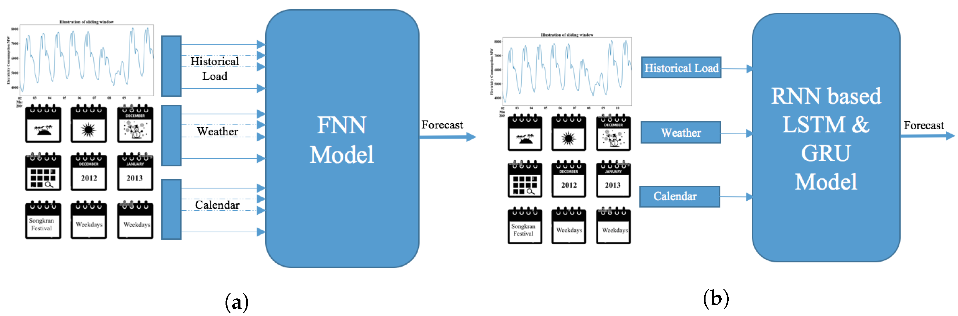
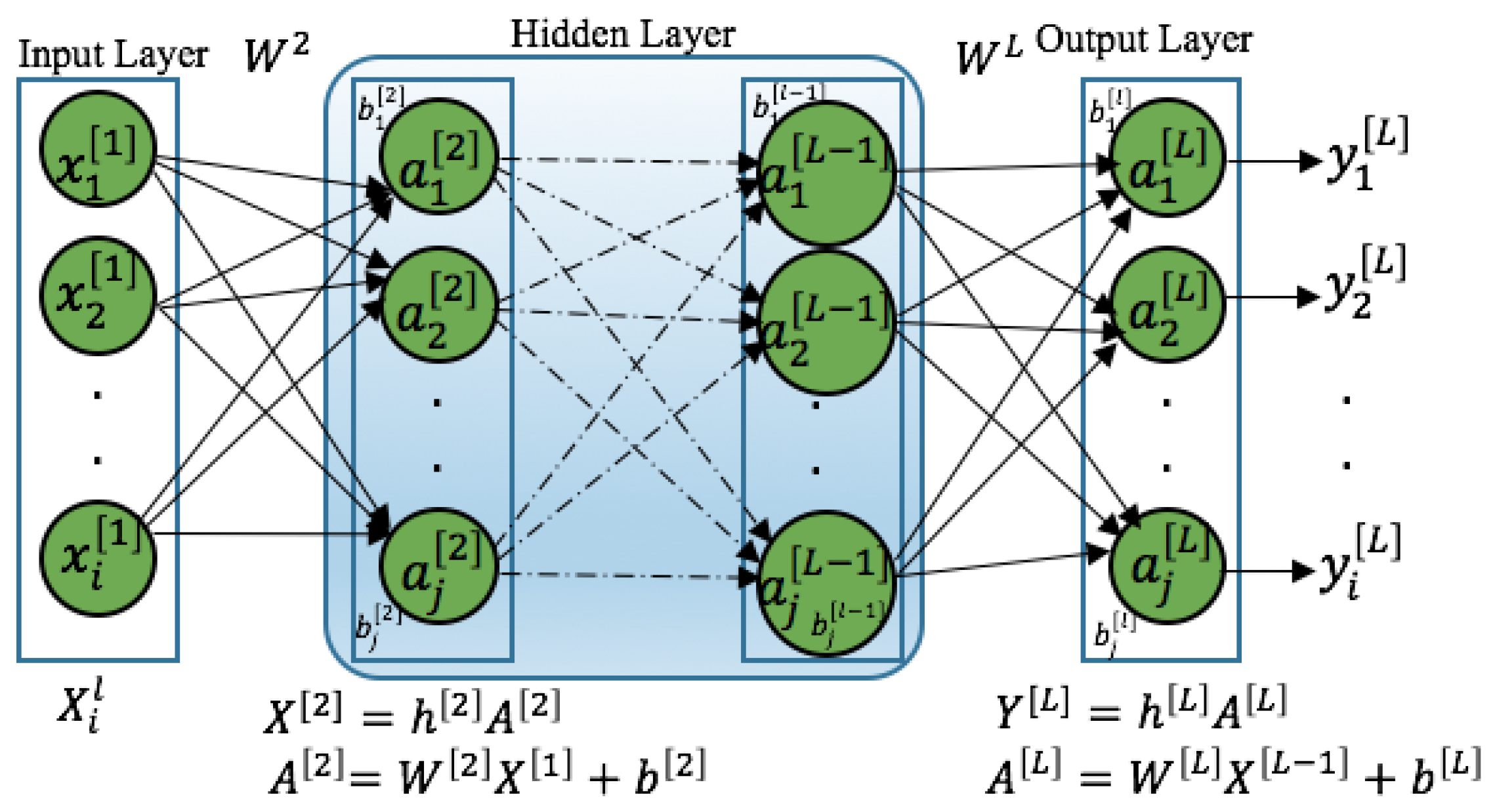
3.1. Feedforward Neural Networks (FNNs)
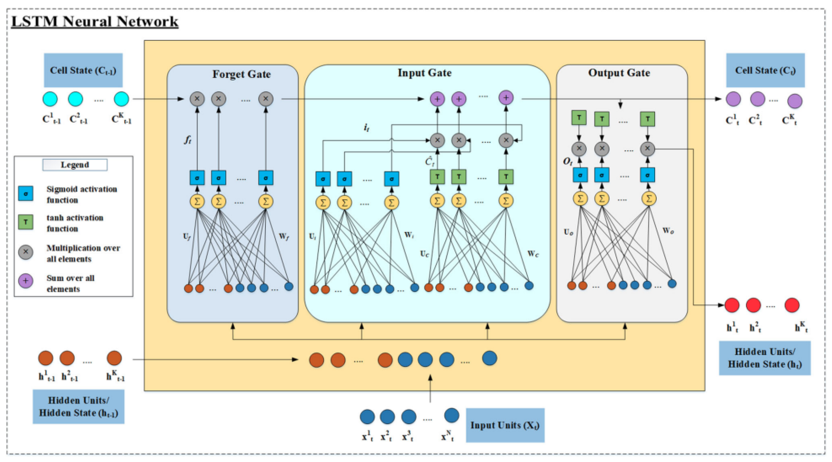
3.2. RNN with Long Short-Term Memory (LSTM)
- 1.
- The forget gate is controlled based on the input and the previous hidden state that decides which of the previous information is to be discarded.
- 2.
- The input gate is the degree to which the new content added to the memory cell is modulated, i.e., selectively read into the information that is controlled based on the input. The weight of the input gate is independent from that of the forget gate.
- 3.
- The output modulates the amount of memory content.
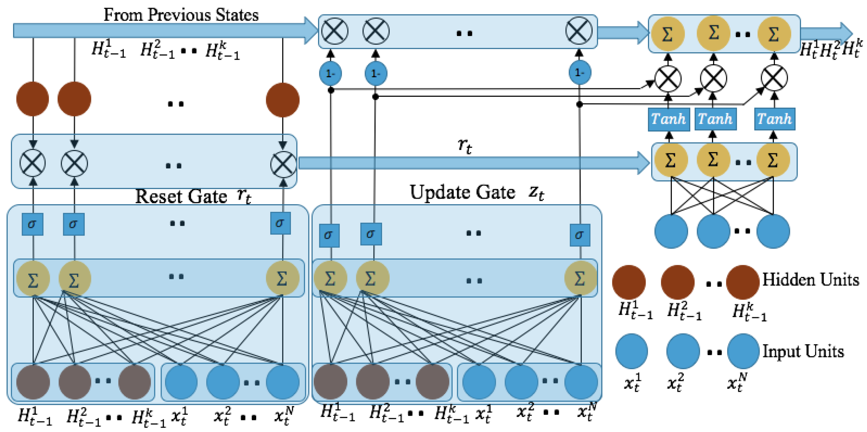
3.3. RNN with Gate Recurrent Unit (GRU)
4. Electricity Demand Profile on Study Area
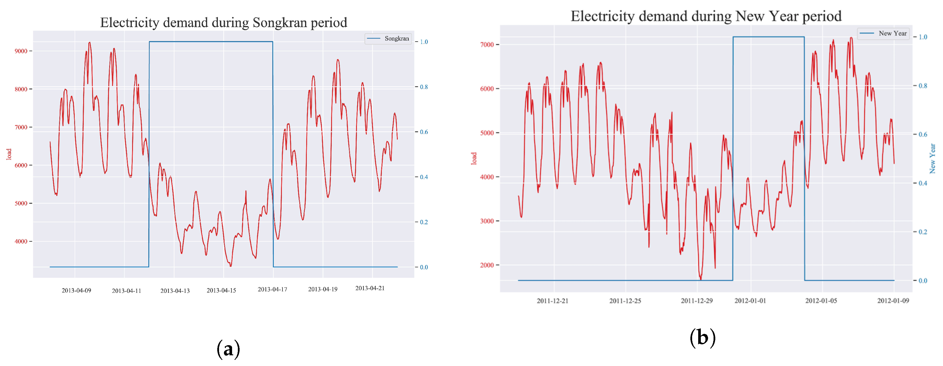
4.1. Seasonal and Holiday Pattern
4.2. Monthly, Weekly, and Daily Patterns
4.3. Temperature
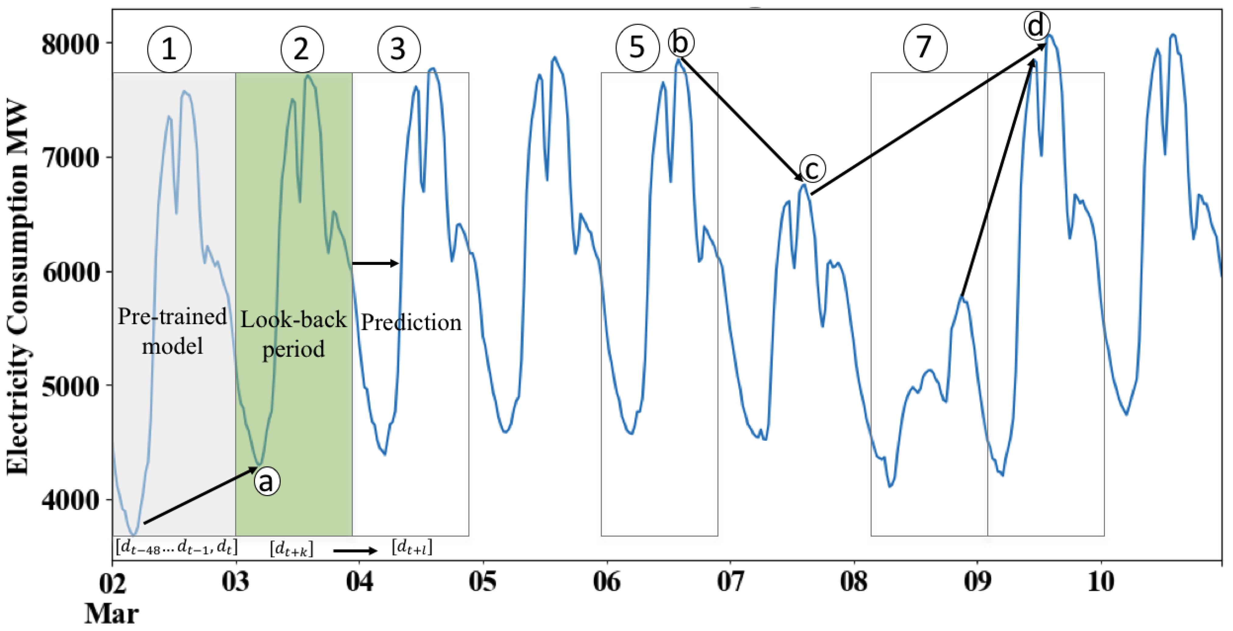
5. Methods
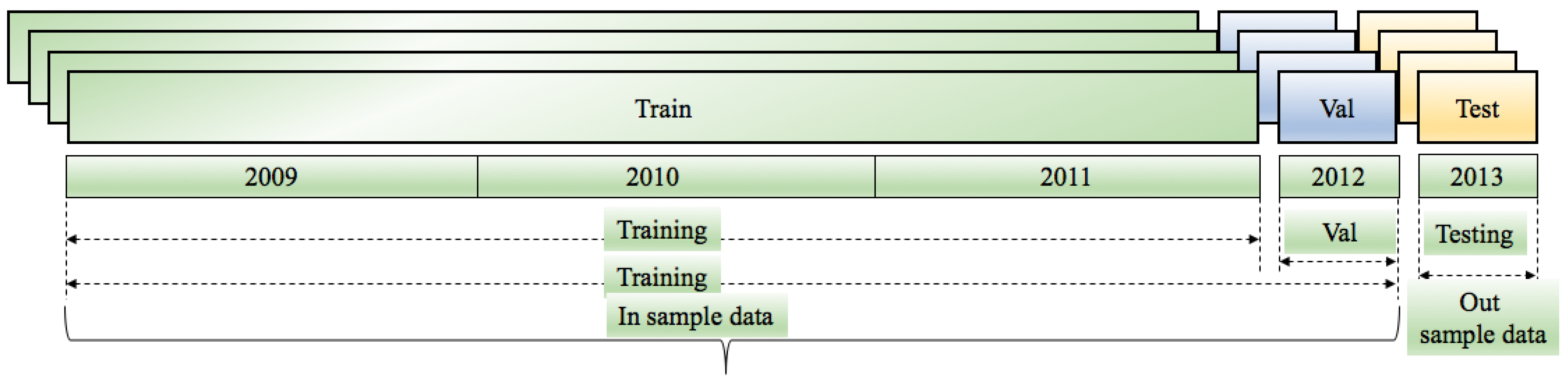
- : demand for working days only; training and validation length 911 days; testing length 239 days.
- : demand for the full dataset;, training length 1365 days; testing length 365 days.

5.1. Feature Selection
5.2. Experimental Setup
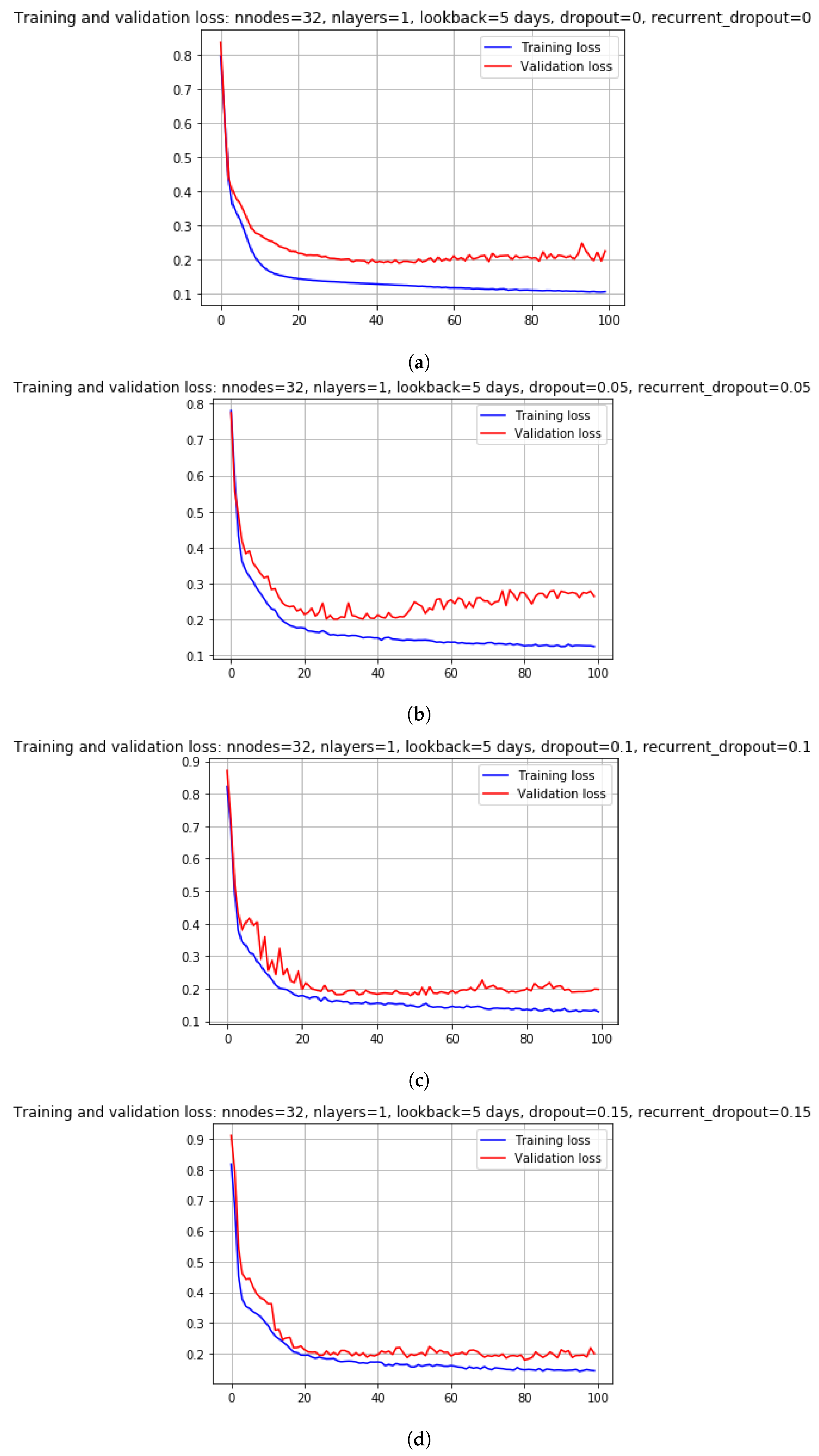
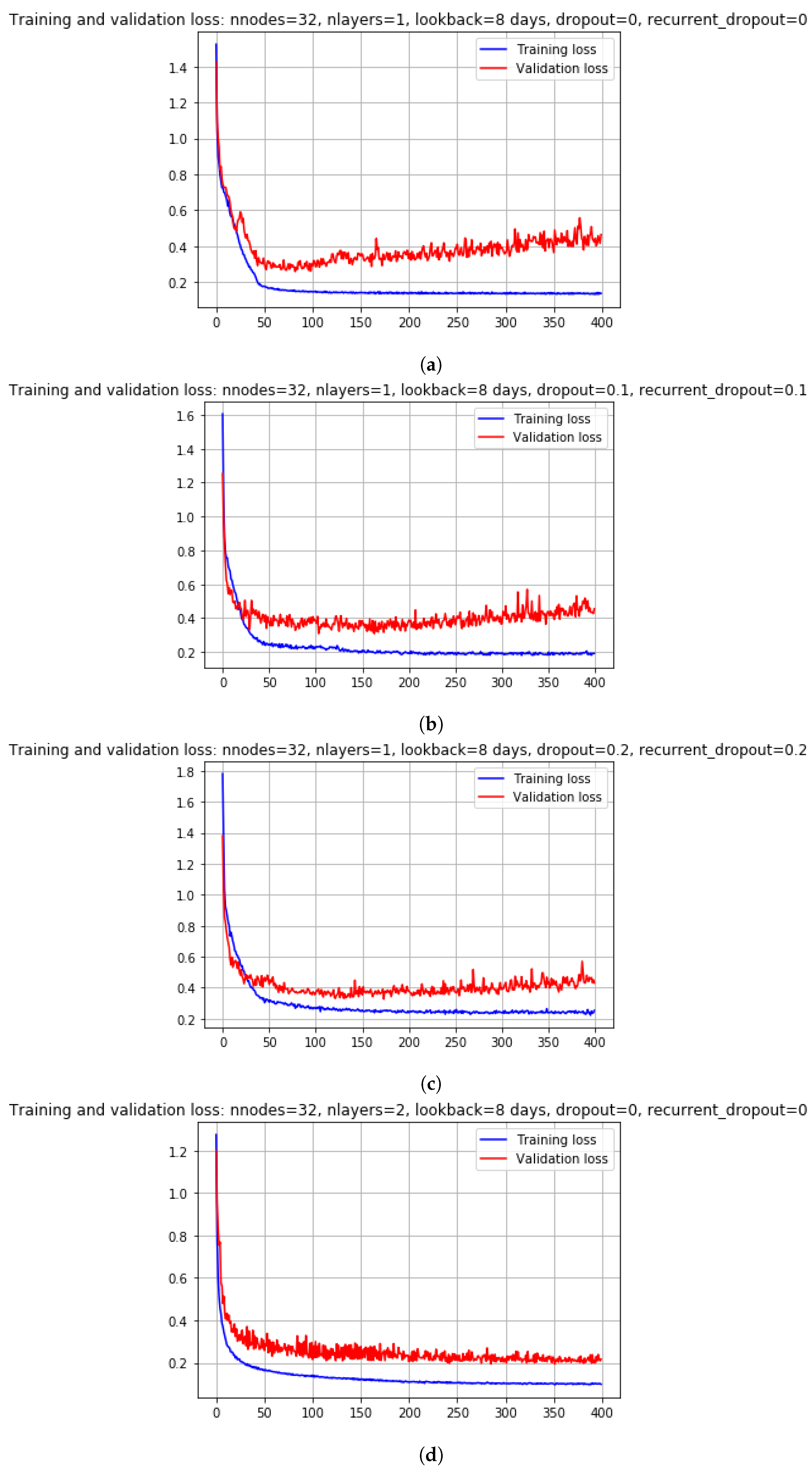
5.3. Hyperparameter Tuning
- Number of hidden layers
- Number of network training iterations
- Mini-batch size that denotes the number of time series considered for each full back propagation for each iteration
- Epochs, which denotes one full forward and backward pass through the whole dataset; the number of epochs denotes the required number of passes over the dataset for optimal training.
- Dropout, which is a technique to prevent the problem of overfitting by excluding the negligibly influenced neurons from the network. We applied both forward and recurrent drop-out.
- Lookback period, which denotes the number of previous timesteps taken to predict the subsequent timestep. In our tuning, we used a 5–10 day lookback period to predict the subsequent timestep of one day ahead.
5.4. Criticism of ANNs
6. Results and Discussion
6.1. Parameter Tuning for Scenario1
6.2. Parameter Tuning for Scenario2
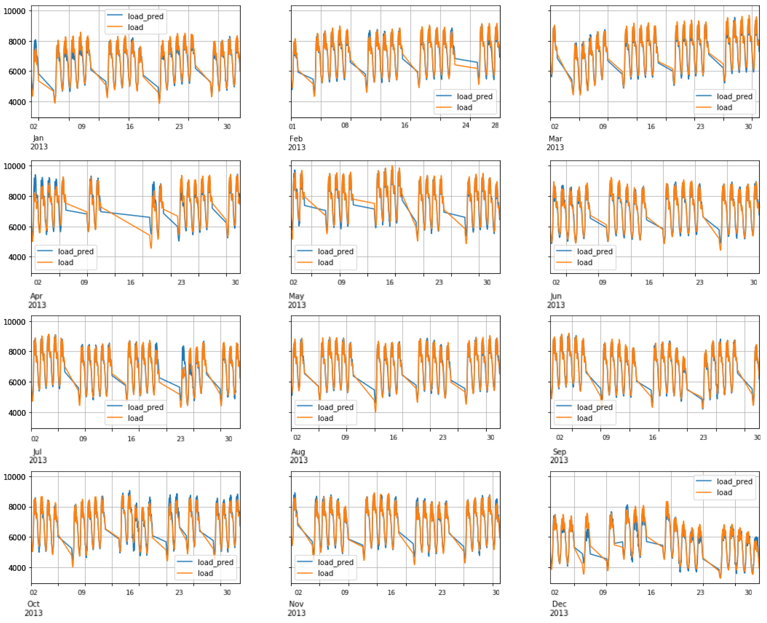
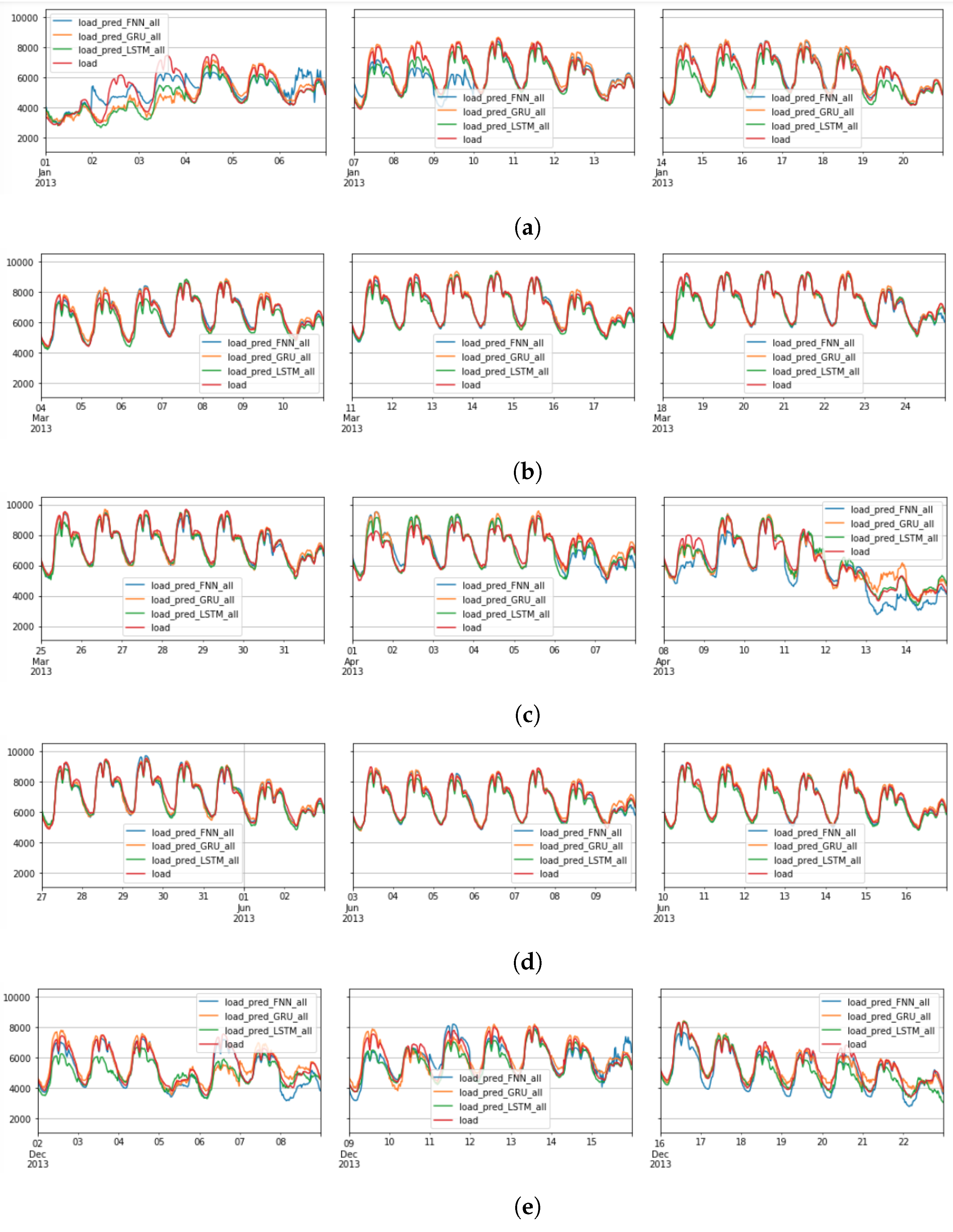
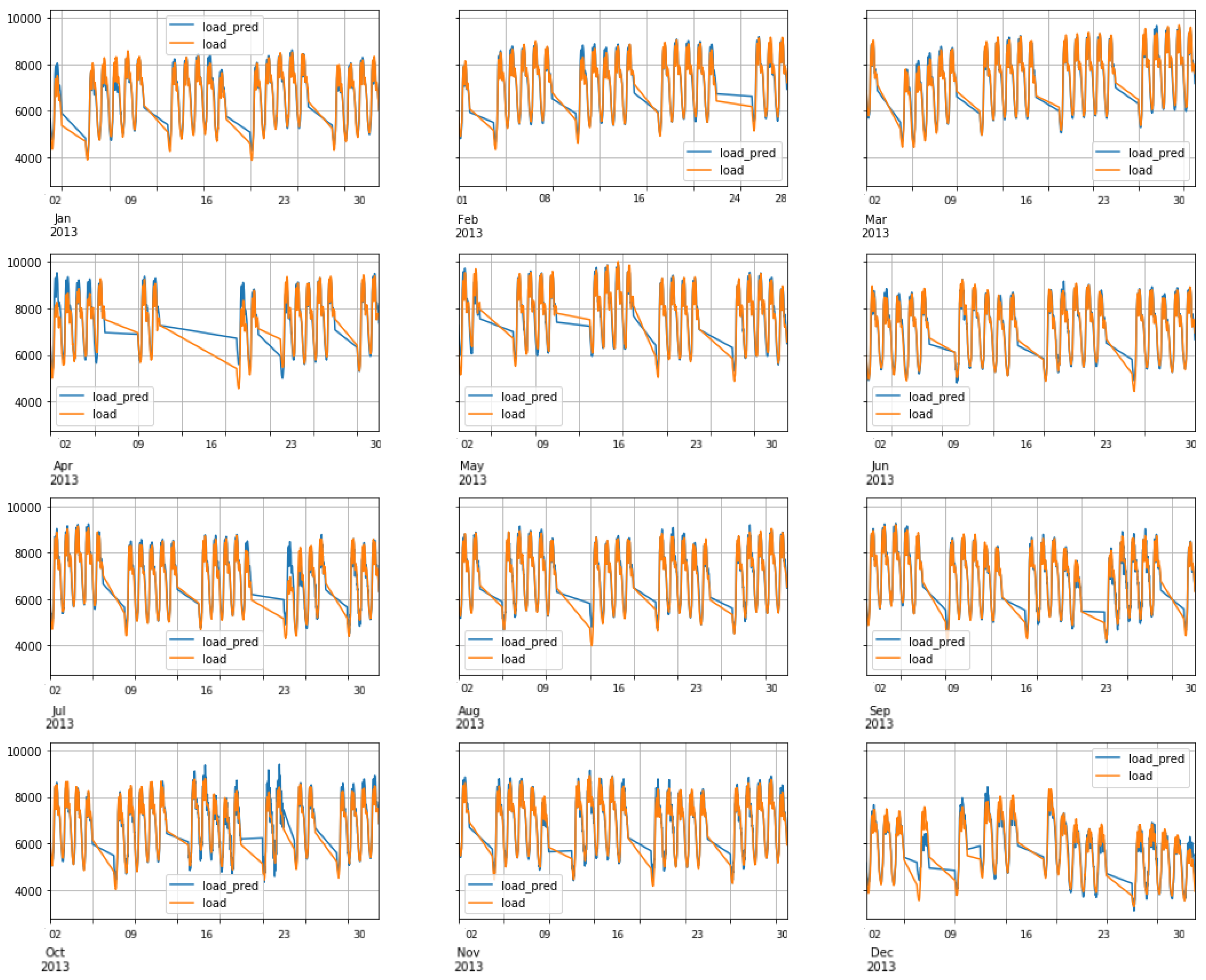
6.3. FNN Performance: Scenario1
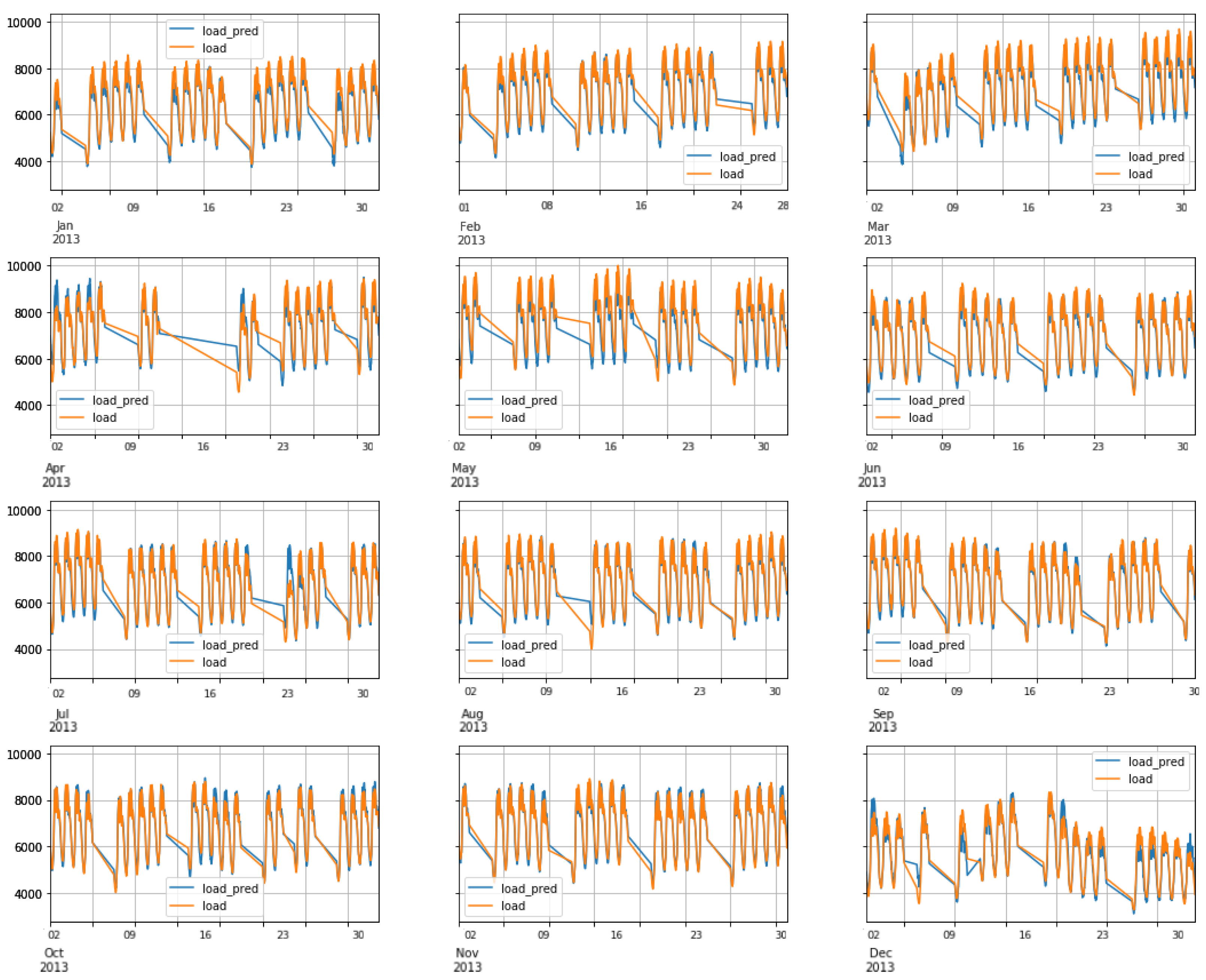
6.4. RNN-LSTM Performance: Scenario1
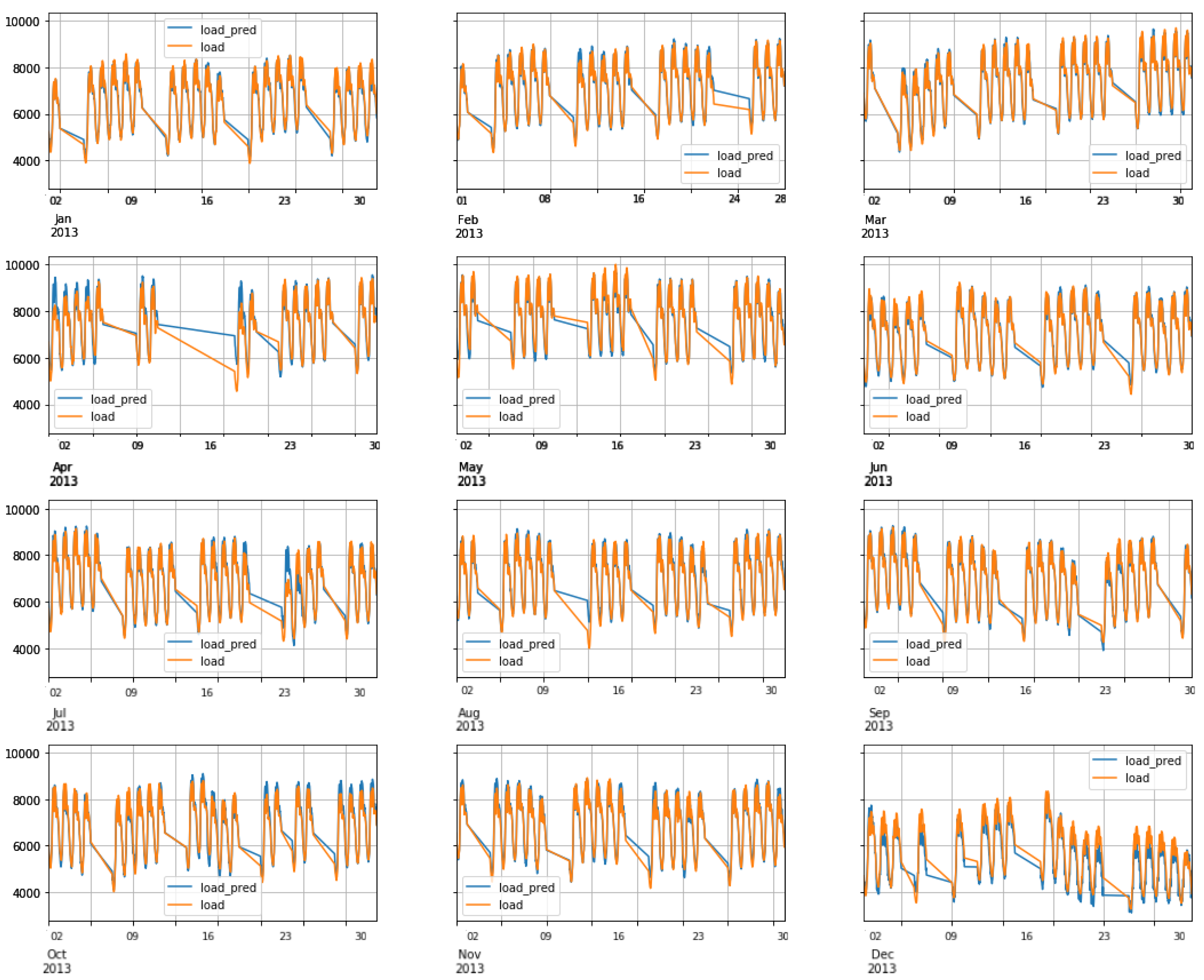
6.5. RNN-GRU Performance: Scenario1
- For the FNN model, the minimum validation loss of 237.82 MWatt was obtained when nnodes = 64, nlayers = 3, lookback = 8 days, dropout = 0, and epochs = 180.
- For the GRU model, the minimum validation loss of 234.22 MWatt occurred when nnodes = 64, nlayers = 2, lookback = 8 days, dropout = 0, and epoch = 99.
- Similarly, for the LSTM model, the minimum validation loss of 242.12 MWatt was achieved when nnodes = 64, nlayers = 2, lookback = 8 days, dropout = 0, and epoch = 56.
7. Conclusions
Author Contributions
Funding
Data Availability Statement
Acknowledgments
Conflicts of Interest
Appendix A. Tuning of Hyperparameters

| Parameters | FNN Results | GRU Results | LSTM Results | ||||||
|---|---|---|---|---|---|---|---|---|---|
| nnodes | nlayers | Look Back | dropout | MAE | epochs | MAE | epochs | MAE | epochs |
| 32 | 1 | 5 | 0 | 226.09 | 319 | 195.31 | 69 | 234.16 | 39 |
| 32 | 1 | 5 | 0.05 | 179.33 | 362 | 204.72 | 72 | 251.48 | 30 |
| 32 | 1 | 5 | 0.1 | 184.27 | 384 | 217.90 | 50 | 223.01 | 50 |
| 32 | 1 | 5 | 0.15 | 205.24 | 327 | 228.40 | 80 | 223.52 | 81 |
| 32 | 1 | 10 | 0 | 264.73 | 196 | NA | NA | NA | NA |
| 32 | 1 | 10 | 0.05 | 231.74 | 302 | NA | NA | NA | NA |
| 32 | 1 | 10 | 0.1 | 196.73 | 399 | NA | NA | NA | NA |
| 32 | 1 | 10 | 0.15 | 197.42 | 348 | NA | NA | NA | NA |
| 32 | 2 | 5 | 0 | 271.67 | 377 | 226.19 | 72 | 200.75 | 51 |
| 32 | 2 | 5 | 0.05 | 259.13 | 136 | 213.24 | 79 | 240.31 | 89 |
| 32 | 2 | 5 | 0.1 | 272.13 | 89 | 235.56 | 57 | 225.07 | 64 |
| 32 | 2 | 5 | 0.15 | 238.8 | 62 | 233.29 | 71 | 224.44 | 100 |
| 32 | 2 | 10 | 0 | 170.41 | 351 | NA | NA | NA | NA |
| 32 | 2 | 10 | 0.05 | 185.37 | 395 | NA | NA | NA | NA |
| 32 | 2 | 10 | 0.1 | 189.83 | 260 | NA | NA | NA | NA |
| 32 | 2 | 10 | 0.15 | 200.49 | 328 | NA | NA | NA | NA |
| 64 | 1 | 5 | 0 | 230.31 | 153 | 221.11 | 79 | 241.49 | 88 |
| 64 | 1 | 5 | 0.05 | 189.14 | 322 | 205.10 | 72 | 214.19 | 40 |
| 64 | 1 | 5 | 0.1 | 255.40 | 307 | 222.80 | 66 | 253.20 | 51 |
| 64 | 1 | 5 | 0.15 | 245.71 | 53 | 207.48 | 78 | 251.50 | 63 |
| 64 | 1 | 10 | 0 | 193.33 | 391 | NA | NA | NA | NA |
| 64 | 1 | 10 | 0.05 | 198.98 | 142 | NA | NA | NA | NA |
| 64 | 1 | 10 | 0.1 | 210.31 | 351 | NA | NA | NA | NA |
| 64 | 1 | 10 | 0.15 | 191.81 | 399 | NA | NA | NA | NA |
| 64 | 2 | 5 | 0 | 314.57 | 140 | 207.66 | 67 | 219.21 | 100 |
| 64 | 2 | 5 | 0.05 | 314.30 | 141 | 227.20 | 61 | 212.24 | 99 |
| 64 | 2 | 5 | 0.1 | 278.63 | 386 | 240.29 | 71 | 218.14 | 67 |
| 64 | 2 | 5 | 0.15 | 293.13 | 126 | 236.68 | 78 | 227.72 | 77 |
| 64 | 2 | 10 | 0 | 220.30 | 356 | NA | NA | NA | NA |
| 64 | 2 | 10 | 0.05 | 192.39 | 340 | NA | NA | NA | NA |
| 64 | 2 | 10 | 0.1 | 218.01 | 365 | NA | NA | NA | NA |
| 64 | 2 | 10 | 0.15 | 216.56 | 349 | NA | NA | NA | NA |
| Parameters | FNN Results | GRU Results | LSTM Results | |||||
|---|---|---|---|---|---|---|---|---|
| nnodes | nlayers | dropout | MAE | epoch | MAE | epoch | MAE | epoch |
| 32 | 1 | 0 | 323.95 | 83 | 269.42 | 71 | 265.85 | 57 |
| 32 | 1 | 0.1 | 387.77 | 164 | 251.01 | 41 | 276.99 | 34 |
| 32 | 1 | 0.2 | 409.22 | 174 | 281.80 | 76 | 267.53 | 55 |
| 32 | 2 | 0 | 243.30 | 352 | 251.17 | 53 | 305.92 | 97 |
| 32 | 2 | 0.1 | 266.86 | 304 | 278.23 | 67 | 274.52 | 97 |
| 32 | 2 | 0.2 | 276.40 | 349 | 280.47 | 99 | 265.23 | 52 |
| 32 | 3 | 0 | 251.37 | 96 | 284.14 | 97 | 306.19 | 58 |
| 32 | 3 | 0.1 | 261.65 | 374 | 293.56 | 98 | 281.66 | 38 |
| 32 | 3 | 0.2 | 273.96 | 209 | 274.05 | 73 | 275.03 | 99 |
| 64 | 1 | 0 | 339.85 | 59 | 263.20 | 82 | 284.72 | 68 |
| 64 | 1 | 0.1 | 327.44 | 51 | 275.22 | 99 | 319.13 | 19 |
| 64 | 1 | 0.2 | 388.25 | 68 | 290.82 | 97 | 269.69 | 43 |
| 64 | 2 | 0 | 243.72 | 324 | 234.22 | 99 | 242.12 | 56 |
| 64 | 2 | 0.1 | 277.33 | 289 | 281.96 | 77 | 254.63 | 97 |
| 64 | 2 | 0.2 | 311.62 | 369 | 296.06 | 80 | 279.30 | 92 |
| 64 | 3 | 0 | 237.82 | 180 | 266.50 | 95 | 296.79 | 88 |
| 64 | 3 | 0.1 | 279.02 | 288 | 286.08 | 92 | 281.90 | 87 |
| 64 | 3 | 0.2 | 296.57 | 66 | 290.56 | 93 | 260.95 | 100 |
References
- Hong, T.; Shu, F. Probabilistic electric load forecasting: A tutorial review. Int. J. Forecast. 2016, 3, 914–938. [Google Scholar] [CrossRef]
- Raza, M.; Khosravi, A. A review on artificial intelligence based load demand forecasting techniques for smart grid and buildings. Renew. Sustain. Energy Rev. 2015, 50, 1352–1372. [Google Scholar] [CrossRef]
- Makridakis, S.; Spiliotis, E.; Assimakopoulus, V. Statistical and machine learning fore- casting methods: Concerns and ways forward. PLoS ONE 2018, 13, e0194889. [Google Scholar] [CrossRef]
- Stosov, M.A.; Radivojevic, N.; Ivanova, M. Electricity Consumption Prediction in an Electronic System Using Artificial Neural Networks. Electronics 2022, 11, 3506. [Google Scholar] [CrossRef]
- Roman-Portabales, A.; Lopez-Nores, M.; Pazos-Arias, J.J. Systematic Review of Electricity Demand Forecast Using ANN-Based Machine Learning Algorithms. Sensors 2021, 21, 4544. [Google Scholar] [CrossRef]
- McCulloch, J.; Ignatieva, K. Forecasting High Frequency Intra-Day Electricity Demand Using Temperature. SSRN Electron. J. 2017. [Google Scholar] [CrossRef]
- Hewamalage, H.; Christoph, B.; Kasum, B. Recurrent Neural Networks for Time Series Forecasting: Current Status and Future Directions. Int. J. Forecast. 2019, 17, 388–427. [Google Scholar] [CrossRef]
- Chapagain, K.; Kittipiyakul, S. Performance Analysis of Short-Term Electricity Demand with Atmospheric Variables. Energies 2018, 11, 818. [Google Scholar] [CrossRef]
- Clements, A.E.; Hurn, A.S.; Li, Z. Forecasting day-ahead electricity load using a multiple equation time series approach. Eur. J. Oper. Res. 2016, 251, 522–530. [Google Scholar] [CrossRef]
- Lusis, P.; Khalilpour, K.; Andrew, L.; Liebman, A. Short-term residential load forecasting: Impact of calendar effects and forecast granularity. Appl. Energy 2017, 205, 654–669. [Google Scholar] [CrossRef]
- Taylor, J.W.; de Menezes, L.M.; McSharry, P.E. A comparison of univariate methods for forecasting electricity demand up to a day ahead. Int. J. Forecast. 2006, 22, 1–16. [Google Scholar] [CrossRef]
- Hong, T.; Wang, P.; Willis, H.L. Short Term Electric Load Forecasting. Int. J. Forecast. 2010, 74, 1–6. [Google Scholar] [CrossRef]
- Bandara, K.; Bergmeir, C.; Smyl, S. Forecasting across time series databases using recurrent neural networks on groups of similar series: A clustering approach. Expert Systems with Applications. Expert Syst. Appl. 2019, 140, 112896. [Google Scholar] [CrossRef]
- Hong, T.; Wang, P. Fuzzy interaction regression for short term load forecasting. Fuzzy Opt. Decis. Mak. 2014, 13, 91–103. [Google Scholar] [CrossRef]
- Dang-Ha, H.; Filippo, M.B.; Roland, O. Local Short Term Electricity Load Forecasting: Automatic Approaches. arXiv 2017, arXiv:1702.08025. [Google Scholar]
- Selvi, M.; Mishra, S. Investigation of Weather Influence in Day-Ahead Hourly Electric Load Power Forecasting with New Architecture Realized in Multivariate Linear Regression & Artificial Neural Network Techniques. In Proceedings of the 8th IEEE India International Conference on Power Electronics (IICPE), Jaipur, India, 13–15 December 2018; pp. 13–15. [Google Scholar]
- Ramanathan, R.; Engle, R.; Granger, C.W.; Vahid-Araghi, F.; Brace, C. Short-run forecasts of electricity loads and peaks. Int. J. Forecast. 1997, 13, 161–174. [Google Scholar] [CrossRef]
- Chapagain, K.; Sato, T.; Kittipiyakul, S. Performance analysis of short-term electricity demand with meteorological parameters. In Proceedings of the 2017 14th Int Conf on Electl Eng/Elx, Computer, Telecom and IT (ECTI-CON), Phuket, Thailand, 27–30 June 2017; pp. 330–333. [Google Scholar]
- Ismail, Z.; Jamaluddin, F.; Jamaludin, F. Time Series Regression Model for Forecasting Malaysian Electricity Load Demand. Asian J. Math. Stat. 2008, 1, 139–149. [Google Scholar] [CrossRef]
- Bouktif, S.; Fiaz, A.; Ouni, A.; Serhani, M. Multi-Sequence LSTM-RNN Deep Learning and Metaheuristics for Electric Load Forecasting. Energies 2020, 13, 391. [Google Scholar] [CrossRef]
- Bouktif, S.; Fiaz, A.; Ouni, A.; Serhani, M. Optimal Deep Learning LSTM Model for Electric Load Forecasting using Feature Selection and Genetic Algorithm: Comparison with Machine Learning Approaches. Energies 2018, 7, 1636. [Google Scholar] [CrossRef]
- Chapagain, K.; Kittipiyakul, S.; Kulthanavit, P. Short-Term Electricity Demand Forecasting: Impact Analysis of Temperature for Thailand. Energies 2020, 13, 2498. [Google Scholar] [CrossRef]
- Cao, Z.; Han, X.; Lyons, W.; O’Rourke, F. Energy management optimisation using a combined Long Short term Memory recurrent neural network-Particle Swarm Optimization model. J. Clean. Prod. 2022, 326, 129246. [Google Scholar] [CrossRef]
- Alya, A.; Ameena, S.A.; Mousa, M.; Rajesh, K.; Ahmed, A.Z.D. Short-term load and price forecasting using artificial neural network with enhanced Markov chain for ISO New England. Energy Rep. 2023, 9, 4799–4815. [Google Scholar] [CrossRef]
- Hongli, L.; Luoqi, W.; Ji, L.; Lei, S. Research on Smart Power Sales Strategy Considering Load Forecasting and Optimal Allocation of Energy Storage System in China. Energies 2023, 16, 3341. [Google Scholar] [CrossRef]
- Hippert, H.S.; Pedreira, C.E.; Souza, R.C. Neural networks for short-term load forecasting: A review and evaluation. IEEE Trans. Power Syst. 2001, 16, 44–55. [Google Scholar] [CrossRef]
- Sankalpa, C.; Kittipiyakul, S.; Laitrakun, S. Short-Term Electricity Load Using Validated Ensemble Learning. Energies 2022, 15, 8567. [Google Scholar] [CrossRef]
- Chapagain, K.; Kittipiyakul, S. Short-term Electricity Load Forecasting Model and Bayesian Estimation for Thailand Data. In Proceedings of the 2016 Asia Conference on Power and Electrical Engineering (ACPEE 2016), Bankok, Thailand, 20–22 March 2016; Volume 55, p. 06003. [Google Scholar]
- Chapagain, K.; Kittipiyakul, S. Short-term Electricity Load Forecasting for Thailand. In Proceedings of the 2018 15th International Conference on Electrical Engineering/Electronics, Computer, Telecommunications and Information Technology (ECTI-CON), Chiang Rai, Thailand, 18–21 July 2018; pp. 521–524. [Google Scholar] [CrossRef]
- Phyo, P.; Jeenanunta, C. Electricity Load Forecasting using a Deep Neural Network. Eng. Appl. Sci. Res. 2019, 46, 10–17. [Google Scholar]
- Su, W.H.; Jeenanunta, C. Short-term Electricity Load Forecasting in Thailand: An Analysis on Different Input Variables. In IOP Conference Series: Earth and Environmental Science; IOP Publishing: Bristol, UK, 2018. [Google Scholar]
- Darshana, A.K.; Chawalit, J. Hybrid Particle Swarm Optimization with Genetic Algorithm to Train Artificial Neural Networks for Short-term Load Forecasting. Int. J. Swarm Intell. Res. 2019, 10, 1–14. [Google Scholar]
- Dilhani, M.H.M.R.S.; Jeenanunta, C. Daily electric load forecasting: Case of Thailand. In Proceedings of the 2016 7th International Conference on Information and Communication Technology for Embedded Systems (IC-ICTES), Bangkok, Thailand, 20–22 March 2016; pp. 25–29. [Google Scholar] [CrossRef]
- Shi, H.; Xu, M.; Li, R. Deep Learning for Household Load Forecasting Novel Pooling Deep RNN. IEEE Trans. Smart Grid 2018, 9, 5271–5280. [Google Scholar] [CrossRef]
- Harun, M.H.H.; Othman, M.M.; Musirin, I. Short term Load Forecasting using Artificial Neural Network based Multiple lags and Stationary Timeseries. In Proceedings of the 2010 4th International Power Engineering and Optimization Conference (PEOCO), Shah Alam, Malaysia, 23–24 June 2010; pp. 363–370. [Google Scholar]
- Tee, C.Y.; Cardell, J.B.; Ellis, G.W. Short term Load Forecasting using Artificial Neural Network. In Proceedings of the 41st North American Power Symposium, Starkville, MS, USA, 4–6 October 2009; pp. 1–6. [Google Scholar]
- Li, Y.; Pizer, W.A.; Wu, L. Climate change and residential electricity consumption in the Yangtze River Delta, China. Proc. Natl. Acad. Sci. USA 2019, 116, 472–477. [Google Scholar] [CrossRef]
- Torabi, M.; Hashemi, S. A data mining paradigm to forecast weather sensitive short-term energy consumption. In Proceedings of the 2012 16th CSI International Symposium on Artificial Intelligence and Signal Processing (AISP 2012), Shiraz, Iran, 2–3 May 2012. [Google Scholar]
- Pramono, S.H.; Rohmatillah, M.; Maulana, E.; Hasanah, R.N.; Hario, F. Deep learning-based short-term load forecasting for supporting demand response program in hybrid energy system. Energies 2019, 12, 3359. [Google Scholar] [CrossRef]
- Kim, T.Y.; Cho, S.B. Predicting residential energy consumption using CNN-LSTM neural networks. Energy 2019, 182, 72–81. [Google Scholar] [CrossRef]
- Qi, Z.; Zheng, X.; Chen, Q. A short term load forecasting of integrated energy system based on CNN-LSTM. Web Conf. 2020, 185, 01032. [Google Scholar] [CrossRef]
- Parkpoom, S.; Harrison, G.P. Analyzing the Impact of Climate Change on Future Electricity Demand in Thailand. IEEE Trans. Power Syst. 2008, 23, 1441–1448. [Google Scholar] [CrossRef]
- Darshana, A.K.; Chawalit, J. Combine Particle Swarm Optimization with Artificial Neural Networks for Short-Term Load Forecasting. Int. Sci. J. Eng. Technol. 2017, 1, 25–30. [Google Scholar]
- Chapagain, K.; Kittipiyakul, S. Short-Term Electricity Demand Forecasting with Seasonal and Interactions of Variables for Thailand. In Proceedings of the 2018 International Electrical Engineering Congress (iEECON), Krabi, Thailand, 7–9 March 2018; pp. 1–4. [Google Scholar]
- Apadula, F.; Bassini, A.; Elli, A.; Scapin, S. Relationships between meteorological variables and monthly electricity demand. Appl. Energy 2012, 98, 346–356. [Google Scholar] [CrossRef]
- Soares, L.J.; Souza, L.R. Forecasting electricity demand using generalized long memory. Int. J. Forecast. 2006, 22, 17–28. [Google Scholar] [CrossRef]
- Sailor, D.; Pavlova, A. Air conditioning market saturation and long-term response of residential cooling energy demand to climate change. Energy 2003, 28, 941–951. [Google Scholar] [CrossRef]
- Machado, E.; Pinto, T.; Guedes, V.; Morais, H. Demand Forecasting Using Feed-Forward Neural Networks. Energies 2021, 14, 7644. [Google Scholar] [CrossRef]
- Gourav, K.; Uday, P.S.; Sanjeev, J. An adaptive particle swarm optimization-based hybrid long short-term memory model for stock price time series forecasting. Soft Comput. 2022, 26, 12115–12135. [Google Scholar] [CrossRef]
- Hong, T.; Xiangzheng, L.; Liangzhi, L.; Lian, Z.; Yu, Y.; Xiaohui, H. One-shot pruning of gated recurrent unit neural network by sensitivity for time-series prediction. Neurocomputing 2022, 512, 15–24. [Google Scholar] [CrossRef]
- Kittiwoot, C.; Vorapat, I.; Anothai, T. Electricity Consumption in Higher Education Buildings in Thailand during the COVID-19 Pandemic. Buildings 2022, 12, 1532. [Google Scholar] [CrossRef]
- Wang, Y.; Niu, D.; Ji, L. Short-term power load forecasting based on IVL-BP neural network technology. Syst. Eng. Procedia 2012, 4, 168–174. [Google Scholar] [CrossRef]
- Cottet, R.; Smith, M. Bayesian Modeling and Forecasting of Intraday Electricity Load. J. Am. Stat. Assoc. 2003, 98, 839–849. [Google Scholar] [CrossRef]
- Shereen, E.; Daniela, T.; Ahmed, R.; Hadi, S.J.; Lars, S.T. Do We Really Need Deep Learning Models for Time Series Forecasting. arXiv 2021, arXiv:2101.02118. [Google Scholar]
- Buitrago, J.; Asfour, S. Short-Term Forecasting of Electric Loads Using Nonlinear Autoregressive Artificial Neural Networks with Exogenous Vector Inputs. Energies 2017, 1, 40. [Google Scholar] [CrossRef]


| Model | MAPE | Prediction Horizon | Data Source | Published Year | Reference |
|---|---|---|---|---|---|
| ANN model | 2.90% | 1 h | DSO, Delhi, India | 2018 | Selvi et al. [16] |
| 1.96% | 1 h | Bandar Abbas, Iran | 2012 | Torabi et al. [38] | |
| CNN-LSTM | 2.02% | 1 h | Public dataset, England, USA | 2019 | Pramono et al. [39] |
| 34.84% | 1 h | UCI ML dataset (households) | 2019 | Kim et al. [40] | |
| 1% | 24 h | Industrial area, China | 2020 | Qi et al. [41] |
| Method | Result | MAPE% | Reference |
|---|---|---|---|
| MLR with AR(2) | Bayesian estimation provides consistent and better accuracy compared to OLS estimation | 1% to 5% | [28] |
| PSO with ANN | Implementing PSO on ANN model outperformed shallow ANN model | 3.44% | [43] |
| OLS | Interation of variable improves the prediction accuracy | >4% | [44] |
| OLS and Bayesian estimation | Including temperature variable in a model can improved the prediction accuracy up to 20% | 2% to 3% | [29] |
| PSO & GA with ANN | PSO+GA outperformed PSO with ANN | >3% | [32] |
| OLS, GLSAR, FNN | OLS and GLSAR models showed better forecasting accuracy than FNN | 1.74% to 2.95% | [22] |
| Ensemble for regression and ML | Lowers the test MAPE implementing blocked Cross Validation scheme. | 2.6% | [27] |
| FNN, RNN based LSTM & GRU | For weekdays and for aggregate data GRU shows better accuracy | 2.47% to 3.44% | In this study |
| Types | Variables | Description |
|---|---|---|
| Deterministic | WD | Week dummy [Mon <Tue … <Sat<Sun] |
| MD | Month dummy [Feb <Mar <… <Nov <Dec] | |
| DayAfterHoliday | Binary 0 or 1 | |
| DayAfterLongHoliday | Binary 0 or 1 | |
| DayAfterSongkran | Binary 0 or 1 | |
| DayAfterNewyear | Binary 0 or 1 | |
| Temperature | Temp | Forecasted temperature |
| MaxTemp | Maximum forecasted temperature | |
| Square temperature | Square of the forecasted temperature | |
| MA2pmTemp | Moving avearage of temperature at 2 pm | |
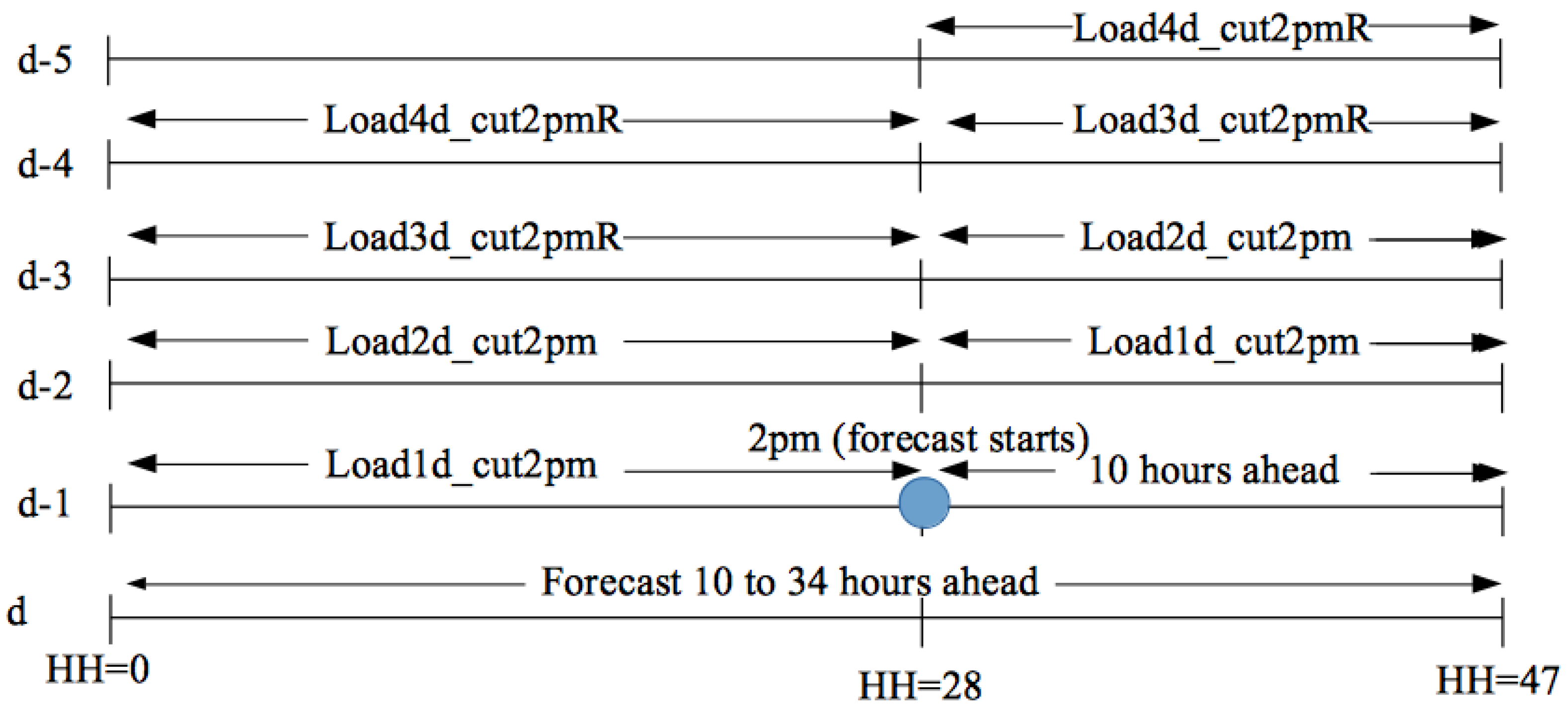
| Lagged | load1d_cut2pm | 1 day ahead until 2 pm and 2 day ahead after 2 pm load |
| load2d_cut2pm | 2 days ahead until 2 pm and 3 day ahead after 2 pm load | |
| load3d_cut2pmR | 3 days ahead until 2 pm and 4 days ahead after 2 pm load | |
| load4d_cut2pmR | 4 days ahead until 2 pm and 5 days ahead after 2 pm load | |
| Interaction | WD:Temp | Interaction: week day dummy to temperature |
| MD:Temp | Interaction: month dummy to temperature | |
| WD:load1d_cut2pm | Interaction: week day dummy to load1d_cut2pm | |
| WD:load2d_cut2pm | Interaction: week day dummy to load2d_cut2pm |
| (a) | |||
| Parameters | Value | ||
| Number of nodes | [2, 4, 8, 16, 32, 64, 128] | ||
| Number of hidden layers | [1 to 5] | ||
| Look back period | [5 days to 10 days] | ||
| Dropout | [0, 0.05, 0.1, 0.15] | ||
| Epochs | [up to 1 million] | ||
| (b) | |||
| Parameters | FNN | LSTM | GRU |
| Time period | 48 | 48 | 48 |
| Delay | 20 | 20 | 20 |
| Pred_batch_size | 48 | 48 | 48 |
| Number of hidden layers | 2 | 1 | 2 |
| Dropout | 0 | 0 | 0 |
| Number of nodes | 32 | 32 | 32 |
| Epochs | 351 | 69 | 51 |
| Look back period | 10 days | 5 days | 5 days |
| Train_fraction | 1 | 1 | 1 |
| Validation loss (MAE) | 170.41 | 195.31 | 200.75 |
| (a) | |||
| Parameters | Value | ||
| Number of nodes | [2, 4, 8, 16, 32, 64, 128] | ||
| Number of hidden layers | [1 to 5] | ||
| Look back period | [5 days to 10 days] | ||
| Dropout | [0, 0.05, 0.1, 0.15] | ||
| Epochs | [up to 1 million] | ||
| (b) | |||
| Parameters | FNN | LSTM | GRU |
| Time period | 48 | 48 | 48 |
| Delay | 20 | 20 | 20 |
| Pred_batch_size | 48 | 48 | 48 |
| Number of hidden layers | 3 | 2 | 2 |
| Dropout | 0 | 0 | 0 |
| Number of nodes | 64 | 64 | 64 |
| Epochs | 180 | 56 | 99 |
| Look back period | 8 days | 8 days | 8 days |
| Train_fraction | 1 | 1 | 1 |
| Validation loss (MAE) | 237.82 | 242.12 | 234.22 |
| Model | nnodes/Layer | nlayers | Look Back | dropout | epoch | Min MAE | Test MAE | Test MAPE(%) |
|---|---|---|---|---|---|---|---|---|
| FNN | 32 | 2 | 10 days | 0 | 351 | 170.41 | 165.54 | 2.47 |
| GRU | 32 | 2 | 5 days | 0 | 51 | 200.75 | 192.76 | 3.37 |
| LSTM | 32 | 1 | 5 days | 0 | 69 | 195.31 | 179.83 | 2.58 |
| Model | nnodes/Layer | nlayers | Look Back | dropout | epoch | Min MAE | Test MAE | Test MAPE(%) |
|---|---|---|---|---|---|---|---|---|
| FNN | 64 | 3 | 8 days | 0 | 180 | 237.82 | 262.8 | 3.54 |
| GRU | 64 | 2 | 8 days | 0 | 99 | 234.22 | 251.3 | 3.44 |
| LSTM | 64 | 2 | 8 days | 0 | 56 | 242.12 | 276.2 | 3.86 |
| Daytype | FNN | GRU | LSTM |
|---|---|---|---|
| Weekdays | 2.97 | 2.71 | 3.76 |
| Weekends | 3.83 | 4.62 | 3.58 |
| Holidays | 9.79 | 6.70 | 6.96 |
| Overall (MAPE %) | 3.54 | 3.44 | 3.86 |
Disclaimer/Publisher’s Note: The statements, opinions and data contained in all publications are solely those of the individual author(s) and contributor(s) and not of MDPI and/or the editor(s). MDPI and/or the editor(s) disclaim responsibility for any injury to people or property resulting from any ideas, methods, instructions or products referred to in the content. |
© 2023 by the authors. Licensee MDPI, Basel, Switzerland. This article is an open access article distributed under the terms and conditions of the Creative Commons Attribution (CC BY) license (https://creativecommons.org/licenses/by/4.0/).
Share and Cite
Chapagain, K.; Gurung, S.; Kulthanavit, P.; Kittipiyakul, S. Short-Term Electricity Demand Forecasting Using Deep Neural Networks: An Analysis for Thai Data. Appl. Syst. Innov. 2023, 6, 100. https://doi.org/10.3390/asi6060100
Chapagain K, Gurung S, Kulthanavit P, Kittipiyakul S. Short-Term Electricity Demand Forecasting Using Deep Neural Networks: An Analysis for Thai Data. Applied System Innovation. 2023; 6(6):100. https://doi.org/10.3390/asi6060100
Chicago/Turabian StyleChapagain, Kamal, Samundra Gurung, Pisut Kulthanavit, and Somsak Kittipiyakul. 2023. "Short-Term Electricity Demand Forecasting Using Deep Neural Networks: An Analysis for Thai Data" Applied System Innovation 6, no. 6: 100. https://doi.org/10.3390/asi6060100
APA StyleChapagain, K., Gurung, S., Kulthanavit, P., & Kittipiyakul, S. (2023). Short-Term Electricity Demand Forecasting Using Deep Neural Networks: An Analysis for Thai Data. Applied System Innovation, 6(6), 100. https://doi.org/10.3390/asi6060100