Article

Raw Material Flow Rate Measurement on Belt Conveyor System Using Visual Data

1
Department of Computer Science, University of the Punjab, Lahore 54590, Pakistan
2
Lucky Core Industries (LCI) Limited, Khewra 49060, Pakistan
3
Intelligent Systems Laboratory & Automation Facility (ISLAF), University of the Punjab, Lahore 54590, Pakistan
*
Author to whom correspondence should be addressed.
Appl. Syst. Innov. 2023, 6(5), 88; https://doi.org/10.3390/asi6050088
Submission received: 21 August 2023 / Revised: 18 September 2023 / Accepted: 28 September 2023 / Published: 30 September 2023
(This article belongs to the Special Issue Towards the Innovations and Smart Factories)

Abstract

:
Industries are rapidly moving toward mitigating errors and manual interventions by automating their process. The same motivation is carried out in this research which targets to study a conveyor system installed in soda ash manufacturing plants. Our aim is to automate the determination of optimal parameters, which are chosen by identifying the flow rate of the materials available on the conveyor belt for maintaining the ratio between raw materials being carried. The ratio is essential to produce 40% pure carbon dioxide gas needed for soda ash production. A visual sensor mounted on the conveyor belt is used to estimate the flow rate of the raw materials. After selecting the region of interest, a segmentation algorithm is defined based on a voting-based technique to segment the most confident region. Moments and contour features are extracted and passed to machine learning algorithms to estimate the flow rate of different experiments. An in-depth analysis is completed on various techniques and convincing results are achieved on the final data split with the best parameters using the Bagging regressor. Each step of the process is made resilient enough to work in a challenging environment even if the belt is placed in an outdoor environment. The proposed solution caters to the current challenges and serves as a practical solution for estimating material flow without manual intervention.

1. Introduction

With the changing face of the world, adopting technology in the industrial processes for the purpose of automation is inevitable. Artificial intelligence (AI) is radically transforming the industrial processes to ensure the mitigation of errors or risks induced by manual interventions, simultaneously allowing the processes to be more structured [1]. The same idea of the digital revolution also inspires our research. The belt conveyor system is an example of a widely used means of transporting a variety of items, especially in the industry, having the capability to carry thousands of tons of material per hour through a simple mechanism [2]. Quantifying the real-time flow of items over the belt is crucial for many use cases; for instance, measuring the flow aids in effective planning, adjusting the speed of the belt or for the effective use of energy, etc. This research targets to study a similar conveyor system installed in the soda ash manufacturing plant at LCI, Khewra Pakistan.
For the production of soda ash, raw materials, such as coke and limestone, are used to generate 40% pure carbon dioxide gas [3]. The process consists of several stages from which the Belt Conveyor is being studied on which the raw materials, i.e., limestone and coke, are transported. First, these materials are carried to a vertical lime kiln where they are heated at a high temperature to produce gas which is further used in soda ash production. The amount of coke mixed with limestone is controlled through a variable-frequency drive (VFD) installed at the source from where coke is passed to the conveyor belt. This drive is used to regulate the flow of coke on the belt because the optimal amount of coke in the mixture of these two substances controls the purity of gas produced through it and makes the production cost-effective. Figure 1 shows a schematic diagram of the environment.
The empirical data revealed that conveyor belt system had been a focus of numerous studies in terms of researching the actual amount of material on belt [4,5,6], tracking the movements [7,8,9], checking for product quality, detecting faults, speed regulation strategy and variable belt-speed energy issue for energy saving [10], etc. These researches discuss various techniques for extracting the material from the belt through computer vision techniques, such as background subtraction, canny edge detection, and morphological operations for analysis and quantification of the material to perform further processes on it to achieve their desired goals [4].
The recent past has witnessed tremendous growth in computer vision which has led to it being widely used in the industry as an automation tool. As righteously quoted by Li and Zhang [1], artificial systems empowered by computer vision are being created to boost the quality and efficiency of production while replacing the need for human intervention. Nowadays, the application of artificial intelligence (AI) in the manufacturing industry covers the areas of product assembly, fault detection, 3D vision system, computer vision-guided Die Cutting, Predictive Maintenance, Safety and Security Standards, Packaging Standards, Barcode Analysis, Inventory Management, and many more, inducing the possibility of increasing the production, controlling downtimes, reducing costs, regulating security and enhancing the quality of production [11].
Taking inspiration from these ideas, several researchers started looking into automating the conveyor belt problems to detect faults, check for product quality, maintain product flow, etc. For instance, Zhou et al. [4] initiated their research on these lines to assess the quantity of material on the belt system and develop an intelligent system that could regulate the speed of the belt accordingly to reduce wastage in terms of energy and equipment. A similar study was put forward to measure the real-time load on a conveyor belt with the help of vision techniques by Shi et al. [12]. It used a system made of a laser generator and camera to gauge the quantity of load from multiple angles by using area proportion and laser-based techniques. The particle velocity of the conveyor system is a determinant of issues that may arise if it is not at its optimal level. In case of an increase in velocity, there is more dust generation, more wear, particle attrition, and more noise. On the contrary, a decrease in velocity results in stagnation zones which causes spillage or blockage. Given the context, it is essential to maintain the particle flow through analysis using techniques, such as the discrete element method (DEM) [13], experimental analysis, and continuum-based analytical methods. In this regard, Hastie & Wypych [14] presented their findings for the methods mentioned above for granular cohesionless techniques. Using high-speed video, they used two continuum-based analytical analyses and captured the conveyor flow. The DEM method was then used to quantify and estimate the particle velocity in a spoon-hood conveyor system.
Ji et al. [10] also analyzed the impact of a conveyor belt system’s speed regulation and energy consumption with variable speed energy-saving controllers related to material flow. They propose an energy saver conveyor belt model with optimal speed regulation for reducing high energy consumption using a polynomial regression-fitting algorithm which applies regression on univariate polynomials and then uses Back Propagation Neural Network Analysis. Karaca & Akinlar [7] built a multi-camera system that tracks the movement of parcels on a conveyor belt after considering its dimensions using stereo cameras. A controller is fed with the corner points’ information, allowing it to arrange the parcels in a line. They use Lucas-Kanade-Tomasi (LKT) algorithms [15,16] for continuous feature tracking in each frame. The technique is further refined with the addition of edge mapping as a post step. Research in [17] explains techniques for volume and size distribution of load transported on a conveyor system. One technique used for data acquisition was the laser triangulation method, which was adopted to acquire the three-dimensional shape of the rock.
A real-time measurement of flow of material on a conveyor belt is proposed in [18]. It used a dual-field measurement system comprised of a couple of light sources to lighten up both the upper and lower surfaces of the belt. On top of that, two binocular cameras are appended to provide a dual field of vision. Tessier et al. [19] discusses an approach to estimate run-of-mine ore composition on a conveyor line system. They explain that the material on the belt varies in size, grindability, and composition. A solution to measure the speed of the belt using computer vision and machine learning techniques is presented in [20]. Given the importance of this task for efficient and secure operation. The focus here is on a contactless solution instead of a conventional setting, which could provide better accuracy as the measuring instrument will not have to deal with flow issues and would avoid wearing off. They adopted a CCD camera to capture the side of the belt. The speed of the belt was obtained by image texture regularity. Wang et al. [21] worked on the problem of detecting belt deviation as belt conveyor systems often face deflection problems in operation. The researchers thus presented a method to use computer vision to detect belt deviation. They use a combination of the Canny edge detector [22], a belt-positioning algorithm founded on the Hough line detection technique [23,24], and morphological processing techniques.
According to the literature cited above, the most research carried out mainly revolves around regulating the speed of conveyor belts, e.g., [4,5,10,20], ensuring the quality [1,11], measuring the quantity [4,12,14], tracking the movement [7] or size of objects [17,19,25] etc., However, it’s important to note that many existing methods depend on the use of high-end devices, including stereo cameras, lasers, speed monitors, and charged-coupled devices, to carry out the necessary experimentation. Dependency on additional devices limits the usage of a solution, given the aspects of availability and affordability of components used. Moreover, the environmental factors also add to the usability of the solution. Through this research, our primary objective is to address a practical challenge encountered by one of the Soda-Ash production plants: specifically, the accurate determination of the flow rate of a mixture on an outdoor conveyor belt. Building upon insights from existing literature, our approach involves automating this process through the application of Computer Vision techniques. By doing so, we aim to achieve several significant advantages, including the ability to conduct experiments more frequently, the elimination of the need for human intervention, and a reduction in the likelihood of errors, ultimately enhancing overall efficiency. Furthermore, our plan is to implement this solution utilizing an easily accessible and simple RGB camera, thereby ensuring a cost-effective and broadly applicable approach.
The rest of the paper is organized as follows. Section 2 explains the whole industrial process and how the data is captured for experimental evaluation. The proposed framework is presented under Methodology in Section 3, which is followed by the Results & Discussion Section 4. Lastly, the Conclusion Section 5 wraps it up by summarizing the findings.

2. Dataset

Before describing the data capturing setup and dataset details, we briefly introduce the industrial process of soda ash production at the experimental site, LCI, Khewra Pakistan.

2.1. Industrial Process

The Kiln plant is used to produce carbon dioxide and calcium oxide from the burning of limestone and coke together in a vertical shaft kiln. Coke burns in the kiln and liberates carbon dioxide and heat. The heat is used further to decompose limestone effectively. The carbon dioxide produced in the kiln is used for carbonation in the monocarbonating and carbonating towers of the Solvay process [26,27], which is the major industrial process for the production of sodium carbonate. Calcium oxide is dissolved with hot water in the rotary dissolver to produce ‘milk of lime’, mainly used in the distillers to recover ammonia. Following are the basic raw materials for kiln operation: Limestone, Coke, and Air (for combustion).

2.1.1. Limestone

Limestone is a sedimentary rock composed mainly of calcite and aragonite, which are crystal forms of calcium carbonate (CaCO3). Limestone is abundantly available from limestone rocks situated within a few miles at Tobar Quarry (Choa Saidan Shah-Khewra, Pakistan). Around 800 to 1200 tons of limestone from Tobar is received daily in trucks of 20–21 ton capacity each. Stones of size between 63.5–127 mm are used in the kilns. The suitability of limestone depends upon its magnesium, silica, and alumina contents.
The stone sizing is analyzed by taking a sample of 20 tons of stone passed through a stencil with two openings. One is 63.5 mm in diameter, and the other is 127 mm in diameter. Stones that pass through a 127 mm opening and are retained on a 63.5 mm opening are considered “Size”. Furthermore, the stones which pass through both openings are considered “Undersize”. Finally, the stones that cannot pass through the 127 mm opening are considered “Oversize”. Physically quality of the stone is inspected by its color, quantity of dust, and size.

2.1.2. Coke

The burning of coke supplies the heat required to decompose calcium carbonate. The size of the coke is kept about half of the size of limestone used, i.e., 35–55 mm. The coke containing high ash percentages is troublesome as ash is composed of heavy metal oxides and silicates. Therefore, the size, quality, moisture content, and calorific value of the coke are essential factors. Coke which is unsorted and has both undersized and oversized particles, is known as Unsorted Coke.
Unsorted coke is processed by crushing and sieving at Coke Sieving Plant. It is fed to Hopper Conveyor, which leads to two vibrating screens. The upper one is 44 mm in size, whereas the lower one is 16 mm in size. Coke which passes through both screens, is called “Undersize” and is collected at the end of the Undersize Conveyor. “Size” coke is the one that passes through the upper screen and is retained on the lower screen. In case any “Oversize” coke does not pass through any of the screens, Coke Crusher and Oversize Conveyor arrangements are also present. This Sorted Coke is transported from the yard to the Coke Bins with the help of dumpers. Dumpers are weighed at the Weigh Bridge to calculate their Gross Weight. The moisture content of the coke is deducted from this weight. Upon exit, the dumper is weighed again, and the net weight of the coke unloaded is then calculated.
A fixed ratio of coke and limestone is maintained using a stone plate feeder stroke and totalizer. Coke and limestone mixture is then sent to the top of kilns via belt conveyor, from where all six top kiln feed bunkers are filled using a tripping trolley. Bunkers are to be filled manually by the belt operator. It is made sure that the Bunker’s level is not less than half.

2.1.3. Experiment Setup

Coke and limestone are kept in the storage bins and open yards as the first part of the process. There is a shed below which coke is stored and moved with the help of loaders. When transferred from their respective bins, limestone and coke are stored in their respective bunkers in the pit. Then, a stone plate feeder is used to drop the limestone from the bunker into the belt conveyor. The strokes of the plate feeder are adjusted to increase or decrease its speed, thus controlling the amount of feed being dropped onto the belt. The limestone experiment is conducted weekly, which helps determine the rate of limestone being charged. Next, coke is fed to the Belt Conveyor, and the time taken for the bunker to get empty is noted down. Based on this experiment coke feed rate is adjusted. The rate of stone changes with the varying stone size, so the stone experiments are carried out every week to have a clear idea about the exact quantity of coke being fed to the kilns. The coke stone ratio is adjusted in a way that the stone per ton ash figure should not exceed the planned amounts.
For this purpose, a variable-frequency drive (VFD) is installed to drop the calculated amount of coke on the belt conveyor. From its panel in the pit, its output can be varied to increase or decrease the amount of feed. The output of the coke ratio controller is adjusted according to the experiment and physical observation of the coke and limestone on the belt. Kiln parameters are also helpful in determining the coke quantity. Coke experiment is carried out daily. Coke is taken into eight bags after every 15 s. These bags are weighed, and the mass is divided by 2 to give the flow of coke in kg/min.
Once on the belt conveyor, the charge, i.e., limestone and coke, in the adjusted ratio from the pit is carried to the top of the kiln. The belt is 1460 ft. in length. There are ten safety switches installed on the belt along with a hardwire running throughout its length, on both ends and parallel to it, which, upon being pulled, forces the belt to stop as it is connected to the safety switches. The two belt drives are used to drive the belt conveyor. One is operational, while the other is always on standby. Drive one usually has a more significant load than Drive two due to the electrical accessories difference between the two drives. The belt takes around 3 min to take the first piece of stone/coke dropped from the pit to the Top Bunker in normal conditions. Detailed specifications of the conveyor belt at the experiment site are presented in Table 1.
Lastly, a tripping trolley is used for coke/stone distribution in all six bunkers. The conveyor belt moves over its rollers, and the coke/stone mixture is put into bunkers via its two chutes. The belt operator appointed at the top of the kiln is responsible for distributing the coke/stone mixture into the desired bunkers. Stone belt conveyor is critical as there is no stand-by for it, and in case of its outage, plant shutdown could occur, so extreme precautions are taken in this operation. The belt operator monitors its running loads and reports to the kiln operator if he finds any abnormality. The top bunkers level is maintained at around half to full. Many other units are involved in the complete process, but they are not included in the scope of our research.

2.2. Data Acquisition

A single-camera is mounted on top of the conveyor belt to capture the dataset. Due to environmental and industrial constraints, it is not precisely on top of the belt instead it is mounted on a pole of the conveyer. The belt operator carries out the weekly experiments and measured flow values are noted for the complete recording. All the experiments took around 30 to 35 min to complete. The primary factor is the amount of coke and limestone carried out on the belt. Hence, we tried to estimate the flow by analyzing the experimental data provided to us. Since the belt conveyor is installed in an outdoor environment, environmental factors such as weather, time of the day, and sunlight affect the quality of the videos, as shown in Figure 2. The dataset was captured using a Samsung high-resolution weatherproof camera as AVI videos over a span of twenty-four weeks. The videos have a resolution of standard definition widescreen video, which is 720 × 576 (16:9). Each video in the dataset is between thirty-five to forty minutes long, where the actual flow rate measurement is spanned over thirty to thirty-five minutes. From a set of twenty videos, sixteen are being used to train the machine learning model and four are being used to test the trained model’s performance.

3. Methodology

The section introduces the proposed framework to estimate the flow rate of limestone and coke being transported from the belt to the top of the Kiln. A visual sensor mounted on top of the conveyor belt is utilized to capture the entire conveyor belt region. This data is used to assess the stone’s quality, the ratio of coke and limestone, issues of belt conveyor, etc. The proposed framework starts by extracting the region of interest to capture only the conveyor belt and discard any unnecessary area around it. Afterward, pre-processing is done to remove any noise from the video frames. Later, considering the challenges of an outdoor environment, limited data, and a single camera, we devised our algorithm to properly segment the material transferred through the conveyor belt. Finally, features are extracted from the segmented region, and machine learning is used to find hidden patterns in the features and estimate the flow rate of the load. The complete process can be visualized in the conceptual map in Figure 3. Each step is described in the following sections.
The implementation of the proposed methodology is done in python by utilizing several libraries for various tasks. Mainly, OpenCV is used for image processing tasks. In addition, Pandas, Numpy, and Scikit-learn are utilized for data analysis and machine learning. Finally, Jupyter Notebook is used as a development environment for better documentation and quick analysis.

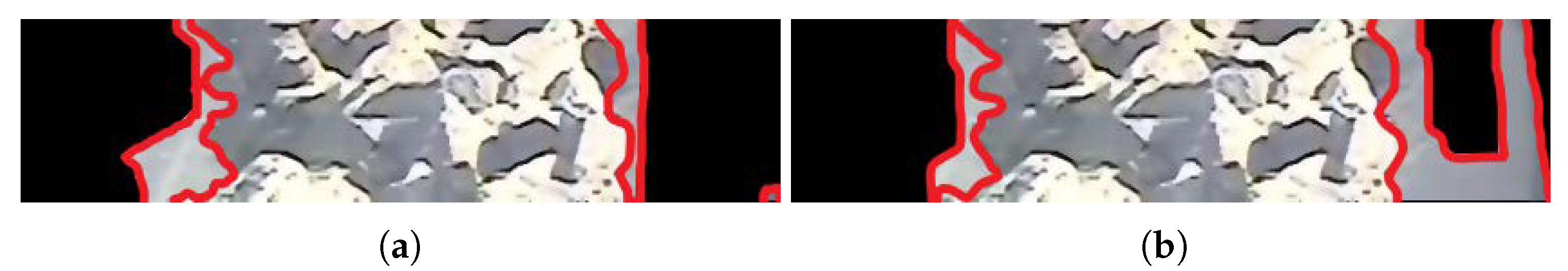
3.1. Extracting Region of Interest

The region of interest (ROI) for our problem is the conveyor belt on which the raw material is carried. Different algorithms can be used for localization by treating conveyor belt edges as straight lines and using algorithms such as Hough transform (HT) [23] to detect these lines. For example, Wang [21] proposed an algorithm based on the Canny edge operator, morphology processing, and Hough line detection to localize the belt-positioning under a complex background environment. Similarly, Dabek [28] also used Hough transform to localize the belt region for automatic conveyor belt maintenance using inspection robots. In our scenario, the camera’s position with respect to the conveyor belt is permanently fixed, making it not only easy for us to extract the region of interest but also computationally very efficient as it does not involve the complex operations like Hough transform, etc. We drew two lines at the boundary of the conveyor belt using OpenCV and extracted the region within those boundaries, which gave us the image mask shown in Figure 4c. Using the image mask, we performed an AND operation of the original image with its prepared masked image, which returns us the region of interest or the surface region of the conveyor belt. Figure 4a shows the original image of the conveyer belt and the lines used to mark the ROI are shown in Figure 4b. Figure 4c shows the masked region and the extracted ROI is shown in Figure 4d.

3.2. Pre-Processing

The conveyor belt is installed in an outdoor environment due to its long length and the materials it carries; hence, the environmental factor varies significantly with the weather and other environmental conditions. Furthermore, being outdoors, the raw material contains much dust and sometimes affects the video quality by adding much noise. Due to this, it is essential to pre-process the data to make sure that the material is fairly visible. For this, a kernel is convolved on an image by computing some function of that pixel and its neighbors, to perform a transformation, such as highlighting or sharpening its edges [29] or removing the noise by blurring the image [30,31]. These transformations serve as features for many machine learning or deep learning tasks, especially in the case of convolution neural networks [32], where it helps the network extract important features. Hence, as a pre-processing step, we first sharpen the image by convolving it using a kernel of size 3 × 3 shown in Figure 5. Convolving the kernel allows us to give a value that best represents the area under that kernel and aids in extracting features of the image.
Sharpening the image helps distinguish the raw material transferred on the belt, providing grounds for better segmentation. However, with sharpening, the noise in the image is also enhanced, which damages the overall quality of the image; thus, blurring is applied to each frame to suppress the noise. Gaussian smoothing [33] is the most famous technique which uses Gaussian distribution as its kernel. The disadvantage of Gaussian blurring is that it blurs the image uniformly, meaning that each region has equal importance. However, in our scenario, the edges of the raw material should be maintained to keep it easily distinguishable. Thus, for this case, we have used the bilateral filtering technique [34] which serves as an advanced version of Gaussian blurring as it maintains the edge information while removing noises. These two differences can be seen in Figure 6. It utilizes the Gaussian distribution values but considers distance and pixel value differences. The bilateral filter starts with linear Gaussian smoothing.
g ( x ) = f G s ( x ) = R f ( y ) G s ( x y ) d y
The weight is only dependent on the spatial distance x y . The bilateral filter adds a weighting term that depends on the total distance f ( y ) f ( x ) . This results in:
g ( x ) = R f ( y ) G s ( x y ) G t ( f ( x ) f ( y ) ) d y R G s ( x y ) G t ( f ( x ) f ( y ) ) d y
The camera is mounted on top of the conveyor belt, which increases its field of vision and makes it capture a lot of unnecessary areas. We also do not need the entire belt region for our study; therefore, we have only selected the region close to the camera. Since the limestone will always be between 63.5–127 mm and coke between 35–55 mm in size, based on this information, given its maximum size limits, we have chosen the optimal region of size 420 × 100 at the end of the belt, which is closest to the camera (see Figure 7). It saves computation as the region to process in a frame has reduced.

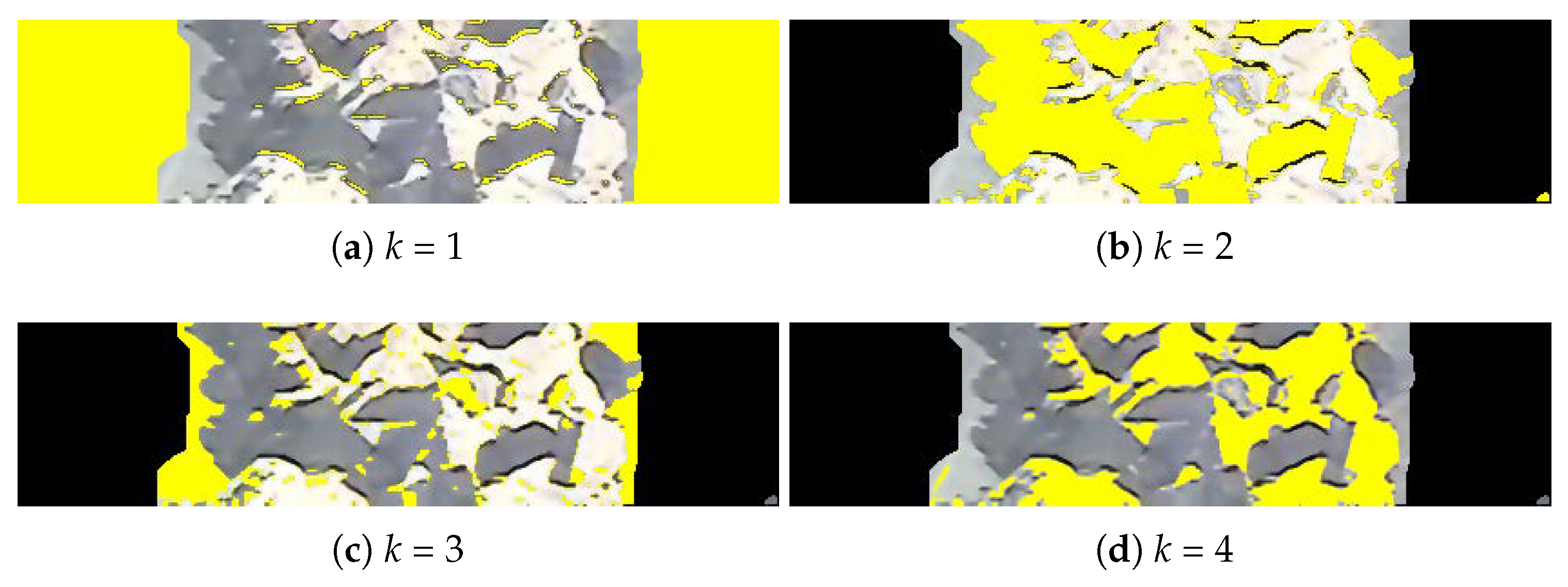
3.3. Coke and Limestone Segmentation

After pre-processing, the next step is to extract coke and limestone being carried on the conveyor belt in each frame. Given the outdoor setup, handling the environmental factors is challenging as each condition can affect the algorithm’s performance. Deep learning is quite famous nowadays due to its high effectiveness in segmenting a challenging and diverse environment [35]. However, the only restriction with deep learning is the huge amount of labeled data [36]. A lot of data needs to be labeled with each relevant class separately before it can be passed as input to the deep learning algorithm. The algorithm can then automatically extracts the relevant features from the raw image it will use to segment the unseen data. We have the image sequences for our problem but do not have the label. Thus, we tried segmenting data using unsupervised deep learning segmentation techniques [37]. In unsupervised segmentation, the algorithm, namely convolutional neural network (CNN) assigns each pixel to the cluster to which it belongs. The pixel labels are clustered together using their feature representations. Unsupervised segmentation works well for examples where objects are easily distinguishable based on color, texture, or other features. Their accuracy can also be increased by giving user input as a scribble [38], which roughly specifies different objects in the image. These scribbles can be used as input to the algorithm. Nevertheless, the environment for our problem is quite challenging. It contains many variable factors in each of our data samples. Even with provided scribble, it struggles to properly distinguish between the conveyor belt and the raw material available on the belt. A resulting segmentation is attached in the Figure 8.
Watershed algorithm [39] is also a widely used technique for segmentation and is especially useful in scenarios where we want to extract objects touching or overlapping. The watershed algorithm uses greyscale images for its segmentation. The greyscale image contains both high and low-intensity values. The watershed algorithm treats the images like a topographic map. The high-intensity values are termed peaks, while low intensities are denoted as valleys. If we fill out each valley with water, the water will rise, and different valleys will start to merge. This is when we build barriers to constitute the object’s boundary, which prevents different valleys from merging. Spread-out objects are easy to identify as they have different intensity values, but heavily clustered objects make it harder to differentiate objects accurately based on intensities. The watershed algorithm produces a set of labels as an output, where each label corresponds to a unique object in the image. The results of the watershed algorithm on our data samples are shown in the Figure 9.
The results look pretty good for the respective frame. However, the algorithm works on the threshold value set to extract the sure foreground region. Therefore, it does not work well for all the data samples as it has different intensity values, negatively impacting the overall segmentation results.
Background Subtraction is another widely used technique for segmentation in which the constant area is termed its background, and the moving instance is identified as its foreground [40]. Background subtraction is used in various applications, such as monitoring, tracking, and recognition of objects, traffic analysis, people detection, tracking of animals, and others [41]. It helps obtain relatively rough and rapid identifications of the objects in the video stream for their further subtle handling. Background subtraction techniques work like our brain; if something does not change, then our brain treats it like a background. The commonly used algorithm for background subtraction is the frame difference [42] method. It takes the absolute difference of two successive frames. So the constant regions in both the frames are termed the background, and the other region is segmented as the image’s foreground. This way of segmenting moving objects in the image works quite well in segmenting the moving environment.
However, in our specific situation, there is an additional challenge. Alongside the raw material on the conveyor belt, there are occasionally dust particles present. The frame difference technique can be sensitive to the choice of threshold, and this sensitivity can lead to some regions of the belt being incorrectly identified as part of the foreground. This issue arises because the dust particles introduce subtle changes in pixel values, which may surpass the threshold and be mistakenly labeled as moving objects.
Apart from the basic frame difference technique, advanced background subtraction methods also exist, which solve the task of foreground extraction by creating a background model. They start by generating a background after processing N frames to provide the background image, then model a technique to keep the background updated for handling the changes that occur over time [43]. Finally, it divides the pixels into sets of background or foreground. Models use different features such as color, texture, and edge descriptors to capture optimal foreground. These features are also called descriptors.
The background model to be finalized is vital as some of the algorithms assume that the background area is static, meaning that the color of the same regions is fixed, and hence background can be identified. However, different illumination variations can distort the colors. Thus, the background model we used must be resilient enough to deal with environmental factors. Given the context, we used the BackgroundSubtractorCNT method [44] due to it being resilient to outdoor lighting conditions. It is also one of the fastest algorithms for background subtraction. The CNT in its name stands for the count, as it counts for how many frames a pixel does not change and divides it into background or foreground.
The algorithm effectively distinguishes the raw material from the conveyor belt, achieving good separation. However, it’s worth noting that some noise may still be present in the output. To address this, we have applied morphological operators to further refine the results. Morphological image processing encompasses a set of operations that pertain to the shape and structure of an image [45]. These operations help us improve the quality and accuracy of the segmentation results.
To eliminate noise from the image, we employ the opening morphological operation [46]. This operation involves two key steps: erosion and dilation. Initially, the image undergoes erosion, followed by dilation, using the same structuring element for both operations. The morphological opening helps remove small objects and thin lines from an image while preserving the shape and size of larger objects in the image. Next, dilation is applied. Morphological dilation makes objects more visible and fills in small holes in objects [47]. As a result, lines appear thicker, and filled shapes appear larger. Finally, to remove its gaps, the closing morphological operation is applied [48]. Morphological closing helps fill small holes in an image while preserving the shape and size of large holes and objects. The closing operation, starts by dilating the image and then proceeds to erode the dilated image, utilizing the same structuring element for both operations. All these transformations are visually depicted in Figure 10.
Following background subtraction and the subsequent application of morphology operations, we successfully isolate the raw material from the conveyor belt. However, it’s essential to acknowledge that this entire technique relies on specific parameters, including the size of the structuring element and the frequency of applying certain morphological operations. Given the variability in environmental conditions across different videos in our dataset, it’s crucial for these parameters to adapt to each unique scenario. For instance, applying the same parameter settings to another example within our dataset could lead to inaccurate results, as illustrated in Figure 11. Therefore, achieving parameter settings that are flexible and adaptable to different scenarios is of utmost importance to ensure the technique’s accuracy and reliability across a diverse range of environmental conditions.
Figure 11 clearly demonstrates that the algorithm’s performance cannot be consistently accurate using fixed thresholds across all data samples. To address this variability, we have developed a voting-based background subtraction technique. This approach focuses on extracting the most confident regions as the foreground. In this technique, we leverage both the frame difference and BackgroundSubtractorCNT methods to extract the image’s foreground. By combining these two approaches and employing a voting mechanism, we enhance the accuracy and robustness of the segmentation process, ensuring that only the most reliable regions are classified as the foreground.
The BackgroundSubtractorCNT method is advantageous because it retains a history of the image, which allows us to filter out subtle changes that might be considered noise in the image. On the other hand, the frame difference technique is sensitive and captures every minor change between two consecutive frames. Given our knowledge that the raw material will consistently be flowing in a specific region on the conveyor belt, by merging these two methods, we effectively preserve the historical information of the target region while eliminating any subtle changes that could occur in a particular frame.
We achieved this by setting the maximum threshold values for the morphological operator so that most of the conveyor belt region would be selected. Then, after both the algorithms select their foreground, we pick only those pixel values detected by both algorithms. These pixels would have the highest confidence of being the foreground as both algorithms detect it. The parameters used to perform morphology are shown in Table 2. Moreover, the structuring element used were rectangle or ellipse, depending upon the condition. A structuring element of size 5 × 5 is shown in Figure 12.
The complete procedure for voting-based segmentation is shown in Figure 13. It shows a single step of the algorithm being performed on an image sequence. The left side of the image shows the output from the frame difference technique. We will call its resulting mask M f d , and the right side shows the output from BackgroundSubtractorCNT, so let its resulting mask be M c n t . After both the algorithms return their resulting masks, we performed the bit-wise AND operation to extract the final output M k .
M k = M f d M c n t
The regions highlighted in red in Figure 14a,b are extracted from the second step of Figure 13. This step illustrates a comparison between the frame difference approach and the CNT method. It’s evident that the frame difference approach outperforms the CNT method in some frames, while in others, the CNT method excels. To address this variability, we have implemented a fusion technique. This technique retains only those pixels that are consistent between both methods, and we’ve introduced a voting-based mechanism to ensure the selection of the correct region.

3.4. Feature Extraction

Once the raw material on the belt is segmented, it can be further processed to extract features for estimating the flow rate. Two techniques are used to extract features; moments information and contour feature information.
One of the most significant features to extract from images is moments [49]. They are useful to describe the object of interest in an image after segmentation in terms of physical properties; for instance, area, eccentricity, orientation, centroid etc. In other words, these scalar quantities have been used in statistics to describe a shape or to quantify the mass distribution [50]. Various orders of moments can be computed which can make the calculations scale invariant, translation invariant and rotation invariant. These features are calculated by taking the weighted average of the pixel intensities, as shown in the formula below:
m = x y I ( x , y )
where I is a grayscale image of size M × N , and 1 x M   1 y N . For our problem, various spatial moments, central moments, and normalized central moments have been used. The spatial moments are used to give information about the object in the image pertinent to its positioning and are computed as follows:
m i j = x y x i y j I ( x , y )
In case of central moments, the origin of the coordinate system is moved to center of gravity or centroid of the object, for the purpose of translational invariance adjustment. These features are computed as follows:
μ i j = x y ( x x ¯ ) i ( y y ¯ ) j I ( x , y )
where x ¯ and y ¯ represent the centroid of the object. Lastly, the normalized central moments factor in the area of object for scaling. Thus, in addition to translational invariance, they become scale invariant as well. The normalized central moments can be calculated as:
ν i j = μ i j μ 00 ( 1 + ( i + j ) 2 )
Contour information [51] is also extracted for each region of the segmented image to achieve better results. As a result of segmentation, the resulting image has four different regions left in it: background, a small portion of the conveyor belt close to the raw material, and the two raw materials, i.e., coke, which is of black color, and limestone in white color. First, k-means image segmentation is used to cluster each region of the image based on its color information [52]. Afterward, we extract area information of these regions using contour. Since most of the region is already segmented, it makes it easy for k-means to segment the regions of interest easily based on their color information.
Based on the information about the image we have, k = 4 seems the optimal choice since we have four regions in the image. With k set to 4, the k-mean clustering performs well to segment each region of the image but still, for the third cluster in Figure 15, there is a region of limestone which is in the same cluster as the conveyor belt. Thus, increasing the total clusters makes segmentation at a more granular level. After clustering, we extract the area of all the clusters and used it along with the moment features. For extracting features, a time window is created to aggregate features of that time period to deal with variable-length data samples.

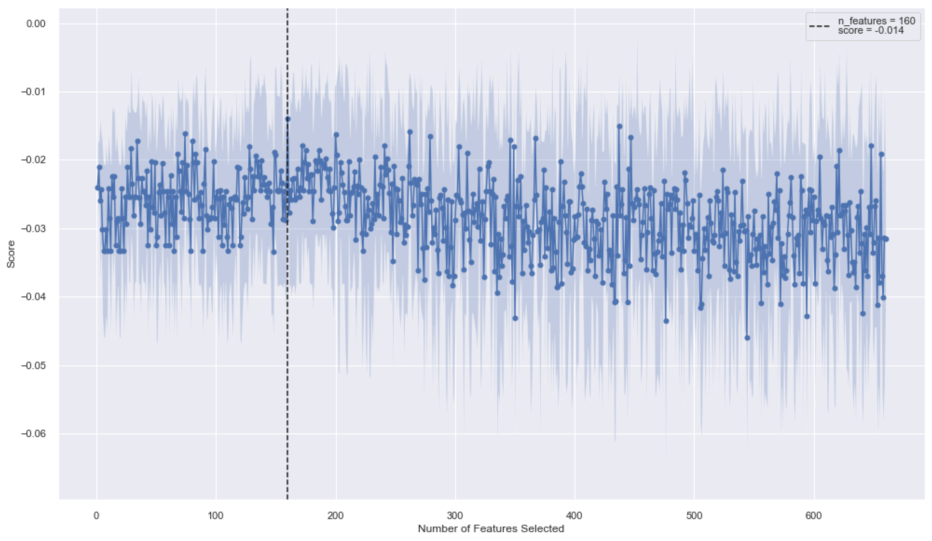
3.5. Feature Selection

We have aggregated features over different length time windows, which contain moments, area, and count information of coke and limestone for each frame. In addition, we have also used feature selection techniques to improve our algorithm’s performance and reduce the computation time of machine learning algorithms. There are multiple ways for feature selection, and some of the most common ones for regression model feature selection are forward, backward, and stepwise.
Forward feature selection [53] begins with no features and then adds the most significant variable. At each subsequent step, it adds features one-by-one into the model until no features are left. In contrast, backward selection [54] begins with all the features and removes the least significant one at each step until none meets the criterion. Finally, the stepwise selection is a mixture of the forward and backward selection techniques. Features are added as described in the forward feature selection, but backward elimination is used for feature elimination after each step. The assumption is that new variables that are better at explaining the dependent variable and variables that are already included may become redundant.
The recursive feature elimination technique is an extension of backward elimination [55]. Recursive feature elimination works on a feature ranking system and is a wrapper-type feature selection technique. In recursive feature elimination, a model is trained on the entire set of features, and an importance score is computed for each predictor variable. Then, the least important predictors are removed from the subset, the model is re-trained, and importance scores are computed again. This process is iterated until the desired number remains. These methods are usually computationally very expensive in case of a large number of features. This is in contrast to filter-based feature selections that score each feature by finding its correlation with the dependent variable and selecting those features with the highest or lowest score.
A significant challenge in feature selection is to decide the number of features to select as it is not known in advance how many features are valid. To find the optimal number of features, cross-validation is used with recursive feature elimination to score different subsets of features and select the best scoring collection of features. We utilized the Decision Tree Regressor as the base estimator for the Recursive Feature Elimination with Cross-Validation technique. The plot in Figure 16 shows the feature selection approach to training data for one of the cross-validation sets. It can be seen that the number of features is added or removed from it iteratively, and a score is calculated at each step. The best negative root mean squared error is achieved with 160 features for that particular training set.

3.6. Machine Learning Algorithms

A large number of machine learning (ML) algorithms have been evaluated to find the best approach. Specifically, as many as nine ML approaches have been tested including decision tree, XGBoos, random forest, bagging regressor, etc. Each is briefly introduced in the following.
  • Decision Tree
    As evident from the name, decision trees form a tree-like structure for performing regression. The decision tree was proposed by Quinlan [56] in 1986. In such an algorithm, the dataset is iteratively broken down into smaller chunks while simultaneously building a tree. It contains a root node representing the complete sample and is further broken down to form further nodes. The inner nodes form data features, and branches represent decision rules. Each data point is passed into the nodes one by one, giving binary answers, which are finally used to give the final prediction.
  • XGBoost
    The XGboost Algorithm, given by Chen et al. [57], refers to Extreme Gradient Boosting, which is an effective and efficient version of the gradient boosting algorithm. It can be used for predictive regression modeling. It originates from the decision trees and belongs to the class of ensemble algorithms; in the boosting category, to be precise. This boosting technique creates decision trees in sequential form and adjusts variable weights to increase the model’s accuracy produced through predecessors.
  • Random Forest
    Another ensemble learning technique, proposed by Breiman [58], comes under the bootstrapping type. The dataset is sampled randomly over a defined number of iterations and variables in bootstrapping. The results of these splits are then averaged out for a better result. It represents a combination of ensemble techniques with a decision tree to attain varied decisions from data. Then these results are averaged out to compute a new result that defines strong results.
  • Bagging Regressor
    An ensemble meta-estimator, also proposed by Breiman [59]. Bagging Regressor fits the fundamental estimator on randomly taken subsets of data, k times, and then combines their predictions through aggregation to attain the final prediction. It indicates that it generates multiple versions of the predictor and utilizes these to get accumulated predictors. These multiple versions are defined by making replicas of the learning set and turning them into new sets for learning. The bagging technique is considered useful because the trees all fit on different data to some extent, which induces differences between them, leading to different predictions. Moreover, its effectiveness is also evident from the fact that it has a low correlation between predictions and prediction errors. We have utilized the DecisionTreeRegressor as the base estimator for our model.
  • Gradient Boosting
    The Gradient Boosting regressor, given by Friedman [60], is another tree-based technique that generates an additive model in a stage-wise manner which in turn allows optimization of random differentiable functions of loss. It uses Mean Squared Error (MSE) as a cost function when used as a regressor. At every stage, fitting of a regression tree is done on the negative gradient of the loss function being used. The technique is used to find a non-linear relationship between the model target and features. Besides, it is good at dealing with outliers, missing values, and high cardinality, regardless of any special treatment.
  • Gamma Regressor
    Gamma regressor proposed by Nelder et al. [61] is a generalized linear model coupled with gamma distribution. These models allow error distribution other than the available normal distribution and help build a linear relationship between predictors and response. Gamma regressors are used for the estimation and prediction of the conditional expectation of some target variable. This model is recommended in case the dependent variable has a positive value.
  • Bayesian Ridge
    Bayesian is a good choice when it comes to situations where data is not properly distributed or is insufficient because it uses probability distributions to formulate linear regressions instead of point estimates. The prediction is not attained as a single value but is estimated through a probability distribution. The implementation used is based on the algorithm described by Tipping [62].
  • RANSAC
    RANdom SAmple Consensus (RANSAC), intrdocued by Fischler et al. [63] is a linear model that handles outliers well, so instead of a complete dataset, it uses a subset of inliers iteratively to estimate the parameters of the model. Furthermore, the outliers are excluded from the training process, thus, eliminating their impact on the learned parameters and coefficients. In terms of implementation, RANSAC uses median absolute deviation to distinguish between outliers and handlers. Moreover, it requires a base estimator to be set for estimations.
  • Theil-Sen Regressor
    Henri Theil [64] and Pranab K. Sen [65] introduced Theil-Sen regressor in 1950 and 1968, respectively which is devised to cater to the outliers. In some instances, the Theil-Sen regressor outperforms RANSAC, a linear regression model. Theil-Sen regressor uses a generalized form of the median in varied dimensions, making it robust to multi-variation outliers. However, this robustness is inversely proportional to dimensionality. Theil-Sen regressor’s performance is comparable to the Ordinary Least Squares for the asymptotic efficiency as an unbiased estimator.

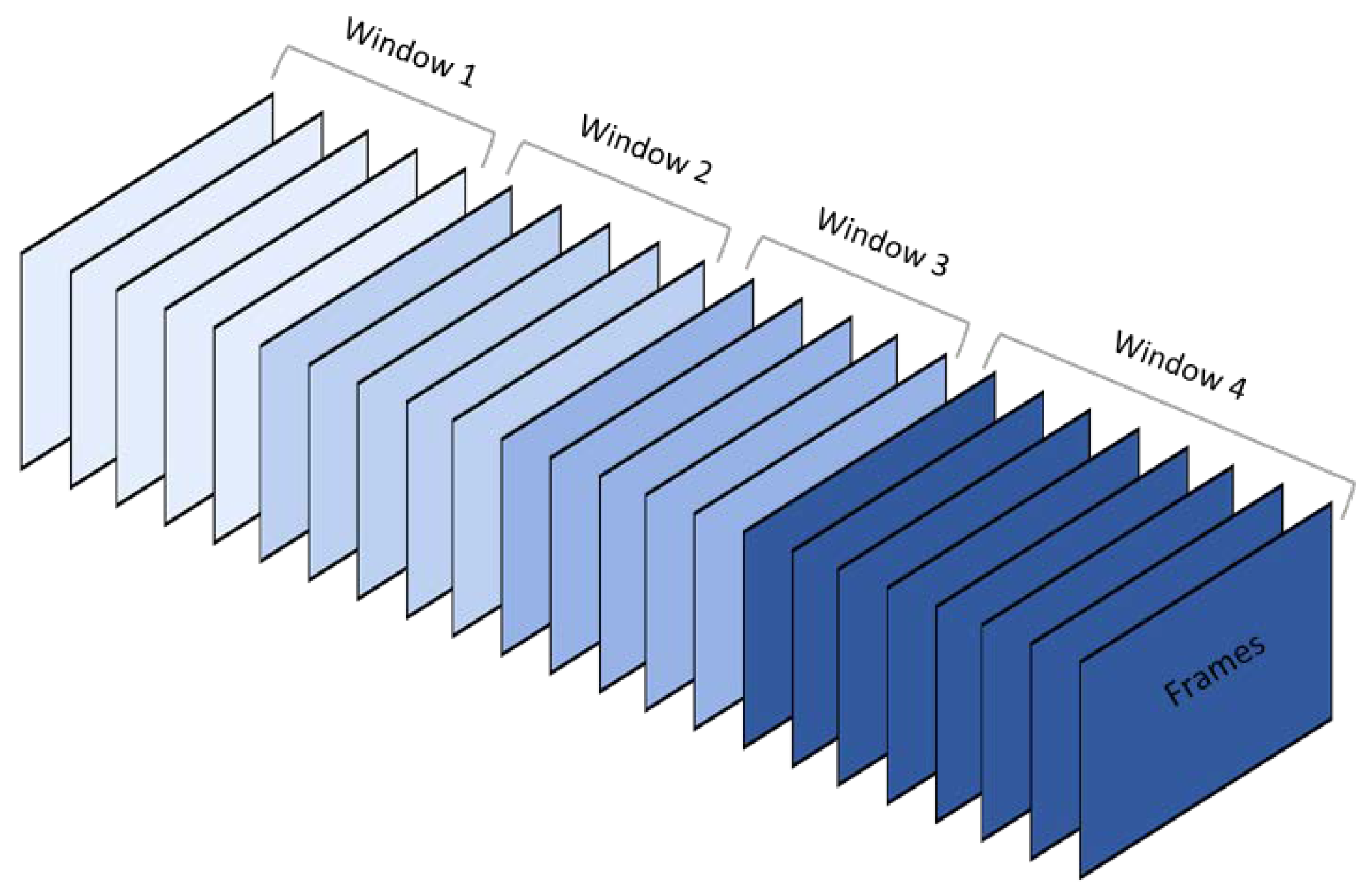
3.7. Window Function

Each sequence in our dataset is of variable length since it depends upon the size and quality of the raw material. So the overall weight and time it runs for on the conveyor belt determine its respective outcome. However, for passing the data to machine learning algorithms, features for all the videos need to be of the same length. Hence, the concept of windows is applied, where features are collected for all video frames, and then aggregation is performed, namely sum and mean, at equal intervals over small subsets of the data.
Furthermore, the total number of windows is selected beforehand, which always produces an equal data length. For instance, if a window is created every minute, all frames within that one-minute time frame are aggregated together. If we perform sum aggregation, all features in a one-minute time frame are summed together. Since we are also deciding the total number of windows, let us say that we only want five windows, then these five windows will only contain data for the first five minutes of the video. However, if the video length exceeds five minutes, the last window will encompass aggregation for all the remaining data. For example, Figure 17 below shows the windows created for a 6 min video.
To summarize, as defined in Section 3.4, the total number of features for a single training example is equal to the number of features multiplied by the number of frames. Since the number of frames for each video is variable, by dividing the features into an equal number of bins, we ensures that our feature vector for all training examples is of equal length.

4. Experimental Evaluations

4.1. Evaluation Metrics

Since we have a regression problem, the metrics we used for performance evaluation include mean absolute error, mean squared error, root mean square error, and mean absolute percentage error. Mean absolute error ( M A E ) measures the average of the absolute values between prediction ( y ^ ) and actual observation (y) over all the instances where all the differences have equal weight. Mean absolute error is less sensitive to outliers.
M A E = 1 N i = 1 n y i y ^ i
where n is the total instances. The mean squared error ( M S E ) tells how good a regression line is to a set of data points. Mean squared error takes the distance of each point to the regression line. After finding the distance, any negative signs are removed by taking the square of these values. It also gives more weight to larger differences from the regression line.
M S E = 1 n i = 1 n y i y ^ i 2
Root mean squared error measures ( R M S E ) the average magnitude of the error. It is the square root of the average squared differences between prediction and actual values. Root mean squared is desirable when large errors are undesirable since it gives higher weightage to large errors. MSE uses the square operation to remove each error value’s sign and punish large errors. The square root reverses this operation, although it ensures that the result remains positive.
R M S E = M S E
The mean absolute percentage error ( M A P E ) is the mean of the absolute percentage errors of predictions. The mean absolute percentage error is scale-independent and is not affected by the global scaling of the target variable. The lower the value for M A P E , the better the machine learning model is at predicting values. The error measurement is more intuitive to understand as a percentage than other measures such as the mean square error because many other error measurements are relative to the range of values.
M A P E = 100 % n i = 1 n y i y i ^ y i

4.2. Results & Discussion

The purpose of the proposed framework is to make the process of measuring the material flow over the belt more efficient, and less prone to error using the mounted visual sensor. The experimental work is carried out to cater the varying environmental scenarios and to eliminate the need for human intervention. The goal is to determine the optimal settings for variable frequency drive and thus, defining the optimal amount of the material being carried on the belt by using image processing and machine learning techniques.
The results are evaluated based on two types of validation, k-fold cross-validation and leave-one-out validation. The cross-validation is used to evaluate the model’s performance on limited data. In k-fold cross-validation, k represents the number of non-overlapping groups or splits into which the data is split. At each iteration, one group is separated as test data. Meanwhile, the rest of the groups are used for training the model. The data is iterated k number of times to test each group of the model and evaluate the model’s performance. This technique gives better confidence in our model performance. For testing our model, we have set the value of k to 5, and the average of all five splits is used as its final metric value. Leave-one-out is also a type of cross-validation, but in this technique each data sample is a separate group, meaning that only one data sample is used as the test data and all other data is used for model training. Leave-one-out is mainly used for a smaller dataset as it is repeated for each example in the dataset. Given our limited data, it represents a suitable choice.
After the features are extracted from the video sequences, the data is split into test train splits using the cross-validation techniques mentioned above. The training set contains the features calculated for each frame of the sample and its respective flow rate value, which serves as our predictor variable. At each iteration, the features are selected from the training data and the model is trained only on the selected features. Then same features are selected for the test dataset, and the model is evaluated further. Finally, we have evaluated the model’s performance with and without the feature selection technique. The figure shows the performance of the trained models based on the parameters defined above on a single test example.
Results are also separately evaluated based on the window size used to aggregate the data and also the type of aggregation used on the data in each window. The three aggregation methods used are sum, mean, and a combination of both sum and mean. In the combination of both sum and mean, the aggregated results from both sum and mean are included as part of the feature vector. Finally, the whole data is evaluated on the best-fitted parameters. The figure demonstrates the results of selected models on different window sizes and the type of aggregation performed.
Machine learning algorithms are also divided into two categories: Linear and non-linear. The non-linear category includes models such as Decision Tree, XGBoost, Random Forest, Bagging Regressor, and Gradient Boosting. On the other hand, the linear models category comprises the Gamma Regressor, Bayesian Ridge, RANSAC, and Theil-Sen Regressor. The primary reason for using Linear models was twofold. Firstly, linear models have a lower risk of overfitting, making them suitable for datasets with limited samples. Secondly, linear models can effectively handle high-dimensional data, where the number of features exceeds the number of samples.
Furthermore, the linear models, including the Gamma Regressor, RANSAC, and Theil-Sen Regressor, have exhibited robustness in dealing with outliers during prediction. Given the existence of numerous outliers in our input data, such as fluctuating lighting conditions and dust, these algorithms emerged as logical choices for the task.
The evaluation of the feature window size involves assessing various parameters, and the outcomes indicate that altering the window size has a substantial impact on the results. A smaller window size accommodates numerous features, which extends training time but yields inaccurate results. Figure 18 shows the results without the feature selection technique, and the plot shows results for windows with 100, 250, 500, 1000, and 2000 frames, respectively. This visualization demonstrates how the model’s accuracy is affected by varying window sizes. Smaller window sizes exhibit higher root mean squared errors, while increasing the window size results in a reduction of the overall error. Notably, the window size of 500 frames consistently produces the most reliable results. All algorithms perform well with this window size, eliminating the need for feature selection.
Figure 19 shows the results with recursive feature selection with Cross-Validation (RFECV) technique in which feature selection is made for each fold separately. The Linear model has shown poor results with the feature selection technique. Apart from the linear models, the windows with sizes greater than 500 frames have performed better for the given parameters. By excluding the linear models, we can say that the window with aggregation performed per 2000 frames has performed the best.
Feature selection serves to reduce the algorithm’s complexity and training time by eliminating non-relevant features based on their scores. However, it’s important to note that sometimes it can have an adverse impact on the overall accuracy of the models. Our findings reveal that none of the linear models, namely the Gamma Regressor, Bayesian Ridge Regressor, and Theil-Sen Regressor, performed well when feature selection was applied, as evidenced in Figure 19. However, the linear models have given a good root mean squared score without the feature selection technique as can be noted from Figure 18. A linear model, the Theil-Sen regressor, gives the best RMSE score for the model training without the feature selection. The results show that feature selection consistently performed better for non-linear models. However, interestingly, the linear models produced the best results without feature selection, reflecting the importance of the complete set of features used for making predictions with the linear models. This observation highlights different behaviors of linear and non-linear models when it comes to feature selection. While non-linear models may benefit from a reduced feature set, linear models demonstrate superior performance when all features are considered. Meanwhile, the boosting methods such as XGBoost, and Gradient Boosting regressor methods have shown mixed results for different parameters such as the size of the window or the aggregation performed on that window. Feature selection does reduce the overall processing speed by excluding unnecessary features, but in our scenario, it comes at the cost of better model accuracy.
The non-linear methods are more flexible and can capture complex relationships between features and the target variable. Feature selection enables the model to focus on the most discriminative features for capturing these non-linear decision boundaries. However, the linear models inherently rely on the linear relationships between features and the target variable, making them less sensitive to irrelevant features. Due to these reasons, we can see from the analysis that linear models are performing slightly better without the feature selection technique compared to the non-linear models.
Choosing the suitable aggregation to perform on the window is also crucial as it impacts the model’s performance and the total number of features used to train the model, impacting its training speed. As discussed, we have performed three aggregation types on each window separately: sum, mean, and a combination of both sum and mean. The sum aggregation performed the worst for small window sizes without any feature selection technique, see Figure 18. However, it performs adequately for large window sizes without the feature selection technique as can be seen from Figure 19. Furthermore, when trained with the feature selection, it performed well on all window sizes. The mean aggregation has shown promising results for linear models without the feature selection technique; however, the rest of the models have not performed very well. However, mean aggregation with feature selection tends to give better accuracy for larger window sizes. Finally, the combination of sum and mean aggregation does not show any significant difference in their performance. However, adding both sum and mean feature increase the overall training time for the models and may add multicollinearity, which undermines the statistical significance of an independent variable.
The leave-one-out validation might work well for small data. However, a similar evaluation is also carried out with k-fold cross-validation and the results using RMSE metric are shown in Figure 20 and Figure 21. The leave-one-out validation can have high variance as its value changes more for different data samples than the value for k-fold cross-validation. So, to maintain the bias-variance ratio, it is also evaluated with k-fold cross-validation.
The mean value of frames in a window has proved to be the most reliable aggregation method in k-fold cross-validation with and without the feature selection technique. However, the sum has given the best results for smaller window sizes. The different machine learning algorithms have shown similar results as the leave-one-out cross-validation. The linear model has performed better without the feature selection, and with feature selection they have produced poor results. The Decision Trees, Random Forest, and Bagging regressor models have produced the best results with the feature selection technique. Without the feature selection technique, the linear models tend to produce better results for larger window sizes. With feature selection, the window size does not have much impact on the final results. The best result for k-fold cross-validation is given by Gamma regressor for 2000 window size without using the feature selection technique.
After analysis, we selected the optimal settings for all the given parameters and trained the machine learning algorithms. The final model was evaluated with a split of training data and test data. For training the final model, the complete dataset was used. For the test set, a new set of input data was utilized, and the model’s performance was reported based on those predictions. The results are shown in Table 3. We have trained our final model without feature selection since the results are better without the feature selection for our problem. Nevertheless, the situation can be changed if the performance is considered more important than accuracy. Apart from it, a window size of 1000 is chosen for performing the mean aggregation function.
The evaluation statistics presented in Table 3 show that the best mean absolute error and mean absolute percentage error are achieved by the Bayesian ridge and the Thiel-Sen regressor, whereas the best mean squared error and root mean squared error is achieved by the Bagging regressor model. To further investigate the performance of all these models, the mean absolute error (MAE) is computed for each of the four test video sequences and the results are presented in Figure 22. These results reaffirm the superior performance of the Thiel-Sen regressor which shows appreciable MAE. The Bayesian ridge also produced good estimates in three tests, however, the difference between the actual (1647 kg/min) and estimated flow rate (1613 kg/min) in the third test video is slightly high. In addition to this error analysis on each test video sequence, we also present the actual and estimated flow rates achieved by our machine learning models on sample test video to show the relative impact of this error. Figure 23 illustrates the performance of the trained models, based on the defined parameters, on a test video 4. In this specific case, the flow rate value for the example was 1637 kg/min, and through the complete procedure, the nearest model predicted its value to be approximately 1639 kg/min. We note from the experimental evaluation that the percentage error is as low as 7% which shows that the proposed framework is reliable in predicting the flow rate of raw material on the belt conveyor system.

5. Conclusions

This paper proposed a comprehensive solution for determining the flow rate of the raw material on the belt conveyor system installed in a Soda-Ash manufacturing plant at LCI Khewra, Pakistan. The flow rate helps us choose the optimal setting for the coke, which is transferred on the conveyor belt through a variable frequency drive. The optimal setting for coke results in optimal gas production and less production waste, which can help save expenditures. We aim to eliminate manual effort by taking the help of an optical lens, making the whole process automatic and making it more efficient and less prone to error.
Since the belt is mounted in an outdoor environment, using an optical lens involved several challenges. However, each part of the algorithm is resilient enough to deal with each type of situation. First, the raw materials are extracted from the conveyor belt by extracting the region of interest, and then segmentation is performed to separate the material from the conveyor belt. The exact position of the conveyor belt and the stable structure on which the camera is placed makes it easy to extract the region of interest. A novel technique was proposed based on background subtraction. The algorithm combines the sequence history and recent changes to extract the foreground region effectively. After the raw material was segmented, different features were computed from the segmented regions, such as moments, color, and information regarding the area of each material. Since each video sequence in the dataset was of variable length, a window technique was used to capture all the information in a fixed-size window which can be further used as an input to the machine learning algorithm. Aggregation was also performed to capture all the information in fewer frames, which helps in reducing complexity. Complexity was also reduced by employing a feature selection technique and testing the model’s performance.
The extracted features were transformed and given as input to different machine learning algorithms. Since we have regression problems, several well-known regression algorithms were used. In terms of model performance, the linear models, namely Gamma regressor, Bayesian Ridge regressor, and Theil-Sen regressor, produced the best results without the feature selection technique. Whereas the Decision Trees, Random Forest performed well with the feature selection technique. Furthermore, the boosting methods such as XGBoost, and Gradient Boosting regressor methods have shown mixed results. The Gradient Boosting algorithm works well with and without feature selection technique, and it also produced the best mean squared error and root mean squared error value for the final run. The techniques were tested with k-fold and leave-one-out cross-validation to maintain the bias-variance trade-off.
The future work includes improving the environment by either developing infrastructure on top of the conveyor belt or installing a high-end optical lens to deal with environmental factors. In addition, the data captured weekly is also being added to the dataset, which may impact the algorithm’s performance; thus, a pipeline needs to be implemented to monitor the model’s performance continuously, and further research can be conducted to optimize the current solution or modify it to cater to the new data.

Author Contributions

Conceptualization, M.S., M.E. and M.H., methodology, M.S., M.S.F., M.E. and M.H.K.; software, M.S., M.S.F., M.E. and M.H.K.; investigation, M.S., M.S.F., M.H., M.H.K. and U.F.; writing—original draft preparation, M.S. and M.S.F., writing—review and editing, M.S., M.S.F. and M.H.K.; visualization, M.S., M.S.F. and U.F., supervision, M.S.F., M.H.K. and U.F. All authors have read and agreed to the published version of the manuscript.

Funding

This research received no external funding.

Institutional Review Board Statement

Not applicable.

Data Availability Statement

Not applicable.

Conflicts of Interest

The authors declare no conflict of interest.

References

  1. Li, Y.; Zhang, Y. Application Research of Computer Vision Technology in Automation. In Proceedings of the 2020 International Conference on Computer Information and Big Data Applications (CIBDA), Guiyang, China, 17–19 April 2020; pp. 374–377. [Google Scholar] [CrossRef]
  2. Rao, D.S. The Belt Conveyor: A Concise Basic Course; CRC Press: Boca Raton, FL, USA, 2020. [Google Scholar]
  3. Simmons, C.W. Manufacture of Soda (Hou, Te-Pan). J. Chem. Educ. 1934, 11, 192. [Google Scholar] [CrossRef]
  4. Zhang, M.; Chauhan, V.; Zhou, M. A machine vision based smart conveyor system. In Proceedings of the Thirteenth International Conference on Machine Vision, Rome, Italy, 2–6 November 2020; Osten, W., Nikolaev, D.P., Zhou, J., Eds.; International Society for Optics and Photonics, SPIE: Bellingham, WA, USA, 2021; Volume 11605, pp. 84–92. [Google Scholar] [CrossRef]
  5. Zeng, F.; Wu, Q.; Chu, X.; Yue, Z. Measurement of bulk material flow based on laser scanning technology for the energy efficiency improvement of belt conveyors. Measurement 2015, 75, 230–243. [Google Scholar] [CrossRef]
  6. Luo, B.; Kou, Z.; Han, C.; Wu, J.; Liu, S. A Faster and Lighter Detection Method for Foreign Objects in Coal Mine Belt Conveyors. Sensors 2023, 23, 6276. [Google Scholar] [CrossRef]
  7. Karaca, H.N.; Akınlar, C. A Multi-camera Vision System for Real-Time Tracking of Parcels Moving on a Conveyor Belt. In Proceedings of the Computer and Information Sciences-ISCIS 2005, Istanbul, Turkey, 26–28 October 2005; Yolum, P., Güngör, T., Gürgen, F., Özturan, C., Eds.; Springer: Berlin/Heidelberg, Germany, 2005; pp. 708–717. [Google Scholar]
  8. Liu, J.; Qiao, H.; Yang, L.; Guo, J. Improved Lightweight YOLOv4 Foreign Object Detection Method for Conveyor Belts Combined with CBAM. Appl. Sci. 2023, 13, 8465. [Google Scholar] [CrossRef]
  9. Hu, K.; Jiang, H.; Zhu, Q.; Qian, W.; Yang, J. Magnetic Levitation Belt Conveyor Control System Based on Multi-Sensor Fusion. Appl. Sci. 2023, 13, 7513. [Google Scholar] [CrossRef]
  10. Ji, J.; Miao, C.; Li, X.; Liu, Y. Speed regulation strategy and algorithm for the variable-belt-speed energy-saving control of a belt conveyor based on the material flow rate. PLoS ONE 2021, 16, e0247279. [Google Scholar] [CrossRef]
  11. Zonta, T.; da Costa, C.A.; da Rosa Righi, R.; de Lima, M.J.; da Trindade, E.S.; Li, G.P. Predictive maintenance in the Industry 4.0: A systematic literature review. Comput. Ind. Eng. 2020, 150, 106889. [Google Scholar] [CrossRef]
  12. Zhang, M.; Zhou, M.; Shi, H. A Computer Vision-Based Real-Time Load Perception Method for Belt Conveyors. Math. Probl. Eng. 2020, 2020, 8816388. [Google Scholar] [CrossRef]
  13. Gröger, T.; Katterfeld, A. Application of the discrete element method in materials handling: Basics and calibration. Bulk Solid Handl. 2007, 27, 17–23. [Google Scholar]
  14. Hastie, D.; Wypych, P. Experimental validation of particle flow through conveyor transfer hoods via continuum and discrete element methods. Mech. Mater. 2010, 42, 383–394. [Google Scholar] [CrossRef]
  15. Lucas, B.D.; Kanade, T. An iterative image registration technique with an application to stereo vision. In Proceedings of the IJCAI’81: 7th International Joint Conference on Artificial Intelligence, Vancouver, BC, Canada, 24–28 August 1981; Volume 2, pp. 674–679. [Google Scholar]
  16. Tomasi, C.; Kanade, T. Detection and Tracking of Point Features; Shape and Motion from Image Streams; School of Computer Science, Carnegie Mellon University: Pittsburgh, PA, USA, 1991. [Google Scholar]
  17. Kontny, M. Machine vision methods for estimation of size distribution of aggregate transported on conveyor belts. Vibroeng. Procedia 2017, 13. [Google Scholar] [CrossRef]
  18. Qiao, W.; Lan, Y.; Dong, H.; Xiong, X.; Qiao, T. Dual-field measurement system for real-time material flow on conveyor belt. Flow Meas. Instrum. 2022, 83, 102082. [Google Scholar] [CrossRef]
  19. Tessier, J.; Duchesne, C.; Bartolacci, G. A machine vision approach to on-line estimation of run-of-mine ore composition on conveyor belts. Miner. Eng. 2007, 20, 1129–1144. [Google Scholar] [CrossRef]
  20. Gao, Y.; Qiao, T.; Zhang, H.; Yang, Y.; Pang, Y.; Wei, H. A contactless measuring speed system of belt conveyor based on machine vision and machine learning. Measurement 2019, 139, 127–133. [Google Scholar] [CrossRef]
  21. Wang, J.; Liu, Q.; Dai, M. Belt vision localization algorithm based on machine vision and belt conveyor deviation detection. In Proceedings of the 2019 34rd Youth Academic Annual Conference of Chinese Association of Automation (YAC), Jinzhou, China, 6–8 June 2019; pp. 269–273. [Google Scholar] [CrossRef]
  22. Canny, J. A Computational Approach to Edge Detection. IEEE Trans. Pattern Anal. Mach. Intell. 1986, PAMI-8, 679–698. [Google Scholar] [CrossRef]
  23. Duda, R.O.; Hart, P.E. Use of the Hough Transformation to Detect Lines and Curves in Pictures. Commun. ACM 1972, 15, 11–15. [Google Scholar] [CrossRef]
  24. Hough, P.V. Method and Means for Recognizing Complex Patterns. US Patent 3,069,654, 18 December 1962. [Google Scholar]
  25. Thurley, M.J. Automated Image Segmentation and Analysis of Rock Piles in an Open-Pit Mine. In Proceedings of the 2013 International Conference on Digital Image Computing: Techniques and Applications (DICTA), Hobart, Australia, 26–28 November 2013; pp. 1–8. [Google Scholar] [CrossRef]
  26. Wikipedia Contributors. Solvay Process—Wikipedia, The Free Encyclopedia. Available online: https://en.wikipedia.org/wiki/Solvay_process (accessed on 23 December 2022).
  27. Johns, R.J. Solvay processes. J. Chem. Educ. 1963, 40, A535. [Google Scholar] [CrossRef]
  28. Dabek, P.; Szrek, J.; Zimroz, R.; Wodecki, J. An Automatic Procedure for Overheated Idler Detection in Belt Conveyors Using Fusion of Infrared and RGB Images Acquired during UGV Robot Inspection. Energies 2022, 15, 601. [Google Scholar] [CrossRef]
  29. Sun, R.; Lei, T.; Chen, Q.; Wang, Z.; Du, X.; Zhao, W.; Nandi, A.K. Survey of Image Edge Detection. Front. Signal Process. 2022, 2. [Google Scholar] [CrossRef]
  30. Schumacher, D.A. II.1—Image Smoothing and Sharpening by Discrete Convolution. In Graphics Gems II; ARVO, J., Ed.; Morgan Kaufmann: San Diego, CA, USA, 1991; pp. 50–56. [Google Scholar] [CrossRef]
  31. Fan, L.; Zhang, F.; Fan, H.; Zhang, C. Brief review of image denoising techniques. Vis. Comput. Ind. Biomed. Art 2019, 2, 7. [Google Scholar] [CrossRef]
  32. O’Shea, K.; Nash, R. An Introduction to Convolutional Neural Networks. arXiv 2015, arXiv:1511.08458. [Google Scholar]
  33. Deng, G.; Cahill, L. An adaptive Gaussian filter for noise reduction and edge detection. In Proceedings of the 1993 IEEE Conference Record Nuclear Science Symposium and Medical Imaging Conference, San Francisco, CA, USA, 31 October–6 November 1993; Volume 3, pp. 1615–1619. [Google Scholar] [CrossRef]
  34. Tomasi, C.; Manduchi, R. Bilateral filtering for gray and color images. In Proceedings of the Sixth International Conference on Computer Vision (IEEE Cat. No.98CH36271), Bombay, India, 7 January 1998; pp. 839–846. [Google Scholar] [CrossRef]
  35. Minaee, S.; Boykov, Y.; Porikli, F.; Plaza, A.; Kehtarnavaz, N.; Terzopoulos, D. Image Segmentation Using Deep Learning: A Survey. IEEE Trans. Pattern Anal. Mach. Intell. 2022, 44, 3523–3542. [Google Scholar] [CrossRef] [PubMed]
  36. Alzubaidi, L.; Zhang, J.; Humaidi, A.J.; Al-Dujaili, A.; Duan, Y.; Al-Shamma, O.; Santamaría, J.; Fadhel, M.A.; Al-Amidie, M.; Farhan, L. Review of deep learning: Concepts, CNN architectures, challenges, applications, future directions. J. Big Data 2021, 8, 53. [Google Scholar] [CrossRef] [PubMed]
  37. Kanezaki, A. Unsupervised Image Segmentation by Backpropagation. In Proceedings of the 2018 IEEE International Conference on Acoustics, Speech and Signal Processing (ICASSP), Calgary, AB, Canada, 15–20 April 2018; pp. 1543–1547. [Google Scholar] [CrossRef]
  38. Lin, D.; Dai, J.; Jia, J.; He, K.; Sun, J. ScribbleSup: Scribble-Supervised Convolutional Networks for Semantic Segmentation. In Proceedings of the 2016 IEEE Conference on Computer Vision and Pattern Recognition (CVPR), Las Vegas, NV, USA, 27–30 June 2016; pp. 3159–3167. [Google Scholar] [CrossRef]
  39. Beucher, S.; Lantuéjoul, C. Use of Watersheds in Contour Detection. In Proceedings of the International Workshop on Image Processing: Real-Time Edge and Motion Detection/Estimation, Rennes, France, 17–21 September 1979; Volume 132, pp. 1–22. [Google Scholar]
  40. Mohan, A.S.; Resmi, R. Video image processing for moving object detection and segmentation using background subtraction. In Proceedings of the 2014 First International Conference on Computational Systems and Communications (ICCSC), Trivandrum, India, 17–18 December 2014; pp. 288–292. [Google Scholar] [CrossRef]
  41. Garcia-Garcia, B.; Bouwmans, T.; Rosales Silva, A.J. Background subtraction in real applications: Challenges, current models and future directions. Comput. Sci. Rev. 2020, 35, 100204. [Google Scholar] [CrossRef]
  42. Singla, N. Motion detection based on frame difference method. Int. J. Inf. Comput. Technol. 2014, 4, 1559–1565. [Google Scholar]
  43. Mubasher, M.M.; Farid, M.S.; Khaliq, A.; Yousaf, M.M. A parallel algorithm for change detection. In Proceedings of the 2012 15th International Multitopic Conference (INMIC), Islamabad, Pakistan, 13–15 December 2012; pp. 201–208. [Google Scholar] [CrossRef]
  44. Zeevi, S. BackgroundSubtractorCNT: A Fast Background Subtraction Algorithm. 2016. Available online: https://zenodo.org/record/4267853 (accessed on 3 October 2022).
  45. Haralick, R.M.; Sternberg, S.R.; Zhuang, X. Image Analysis Using Mathematical Morphology. IEEE Trans. Pattern Anal. Mach. Intell. 1987, 9, 532–550. [Google Scholar] [CrossRef]
  46. Jamil, N.; Sembok, T.M.T.; Bakar, Z.A. Noise removal and enhancement of binary images using morphological operations. In Proceedings of the 2008 International Symposium on Information Technology, Kuala Lumpur, Malaysia, 26–28 August 2008; Volume 4, pp. 1–6. [Google Scholar] [CrossRef]
  47. Raid, A.; Khedr, W.; El-Dosuky, M.; Aoud, M. Image restoration based on morphological operations. Int. J. Comput. Sci. Eng. Inf. Technol. (IJCSEIT) 2014, 4, 9–21. [Google Scholar] [CrossRef]
  48. Zhang, D. Extended Closing Operation in Morphology and Its Application in Image Processing. In Proceedings of the 2009 International Conference on Information Technology and Computer Science, Kiev, Ukraine, 25–26 July 2009; Volume 1, pp. 83–87. [Google Scholar] [CrossRef]
  49. Wikipedia contributors. Image Moment—Wikipedia, The Free Encyclopedia. Available online: https://en.wikipedia.org/wiki/Image_moment (accessed on 23 December 2022).
  50. Flusser, J.; Zitova, B.; Suk, T. Moments and Moment Invariants in Pattern Recognition; Wiley Publishing: New York, NY, USA, 2009. [Google Scholar]
  51. Gong, X.Y.; Su, H.; Xu, D.; Zhang, Z.; Shen, F.; Yang, H.B. An Overview of Contour Detection Approaches. Int. J. Autom. Comput. 2018, 15, 1–17. [Google Scholar] [CrossRef]
  52. Dhanachandra, N.; Manglem, K.; Chanu, Y.J. Image Segmentation Using K -means Clustering Algorithm and Subtractive Clustering Algorithm. Procedia Comput. Sci. 2015, 54, 764–771. [Google Scholar] [CrossRef]
  53. Ververidis, D.; Kotropoulos, C. Sequential forward feature selection with low computational cost. In Proceedings of the 2005 13th European Signal Processing Conference, Antalya, Turkey, 4–8 September 2005; pp. 1–4. [Google Scholar]
  54. Abe, S. Modified backward feature selection by cross validation. In Proceedings of the 13th European Symposium on Artificial Neural Networks, ESANN, Bruges, Belgium, 27–29 April 2005; pp. 163–168. [Google Scholar]
  55. Guyon, I.; Weston, J.; Barnhill, S.; Vapnik, V. Gene Selection for Cancer Classification using Support Vector Machines. Mach. Learn. 2002, 46, 389–422. [Google Scholar] [CrossRef]
  56. Quinlan, J.R. Induction of decision trees. Mach. Learn. 1986, 1, 81–106. [Google Scholar] [CrossRef]
  57. Chen, T.; Guestrin, C. XGBoost: A Scalable Tree Boosting System. In Proceedings of the KDD ’16: Proceedings of the 22nd ACM SIGKDD International Conference on Knowledge Discovery and Data Mining, San Francisco, CA, USA, 13–17 August 2016; ACM: New York, NY, USA, 2016; pp. 785–794. [Google Scholar] [CrossRef]
  58. Breiman, L. Random Forests. Mach. Learn. 2001, 45, 5–32. [Google Scholar] [CrossRef]
  59. Breiman, L. Bagging predictors. Mach. Learn. 1996, 24, 123–140. [Google Scholar] [CrossRef]
  60. Friedman, J.H. Greedy function approximation: A gradient boosting machine. Ann. Stat. 2001, 29, 1189–1232. [Google Scholar] [CrossRef]
  61. Nelder, J.A.; Wedderburn, R.W.M. Generalized Linear Models. J. R. Stat. Soc. Ser. A (Gen.) 1972, 135, 370–384. [Google Scholar] [CrossRef]
  62. Tipping, M. Sparse Bayesian Learning and the Relevance Vector Machine. J. Mach. Learn. Res. 2001, 1, 211–244. [Google Scholar]
  63. Fischler, M.A.; Bolles, R.C. Random Sample Consensus: A Paradigm for Model Fitting with Applications to Image Analysis and Automated Cartography. Commun. ACM 1981, 24, 381–395. [Google Scholar] [CrossRef]
  64. Theil, H. A rank-invariant method of linear and polynomial regression analysis. Indag. Math. 1950, 12, 173. [Google Scholar]
  65. Sen, P.K. Estimates of the Regression Coefficient Based on Kendall’s Tau. J. Am. Stat. Assoc. 1968, 63, 1379–1389. [Google Scholar] [CrossRef]
Figure 1. Schematic diagram of a conveyor system installed in the soda ash manufacturing industry.
Asi 06 00088 g001
Figure 2. Variation in dataset video quality: good image quality (a), captured at evening time (b), and dusty image (c).
Asi 06 00088 g002
Figure 3. Conceptual map of the proposed framewrk.
Asi 06 00088 g003
Figure 4. (a) Original image, (b) Lines drawn to separate the region of interest, (c) Masked region inside the lines and, (d) Extracted region.
Asi 06 00088 g004
Figure 5. Kernel used for image sharpening in pre-processing step.
Asi 06 00088 g005
Figure 6. Image blurring results on a sample frame from the dataset using a Gaussian blur kernel (a) and bilateral filtering (b).
Asi 06 00088 g006
Figure 7. Selected region for processing.
Asi 06 00088 g007
Figure 8. Poor Segmentation with a deep learning algorithm: (a) original frame, (b) segmentation results using deep learning.
Asi 06 00088 g008
Figure 9. Segmentation results of Watershed algorithm: (a) sample frame from dataset, (b) segmentation results.
Asi 06 00088 g009
Figure 10. (a) Background subtraction using CNT, (b) noise removal using open morphology, (c) filled shapes using dilation operation, and (d) close gaps using dilation operation close.
Asi 06 00088 g010
Figure 11. Poor segmentation results using the same parameters for different environment.
Asi 06 00088 g011
Figure 12. Rectangular structuring element (left), and ellipse structuring element (right).
Asi 06 00088 g012
Figure 13. Flowchart of proposed end-to-end segmentation algorithm.
Asi 06 00088 g013
Figure 14. (a) Extra region segmented by frame difference, (b) extra region segmented by background subtraction on sample input frame.
Asi 06 00088 g014
Figure 15. K-means segmentation results with different values of k.
Asi 06 00088 g015
Figure 16. Feature selection with recursive feature elimination with cross-validation (RFECV).
Asi 06 00088 g016
Figure 17. Window function concept: dividing the video into smaller equal size chunks, except the last which might contain the leftover frames not enough to form a complete chunk.
Asi 06 00088 g017
Figure 18. Leave-one-out results without recursive feature engineering.
Asi 06 00088 g018
Figure 19. Leave-one-out results with recursive feature engineering.
Asi 06 00088 g019
Figure 20. K-fold results without recursive feature engineering.
Asi 06 00088 g020
Figure 21. K-fold results with recursive feature engineering.
Asi 06 00088 g021
Figure 22. Absolute error between the estimated and the actual flow rates (kg/min) on test dataset.
Asi 06 00088 g022
Figure 23. Flow rate prediction using different machine learning (ML) models versus the actual flow rate.
Asi 06 00088 g023
Table 1. Specification of the conveyor belt at the experiment site.
PropertyValue
Motor Power40 HP
Speed1465 RPM
Length1460 feet
Small rollers510 units
Return rollers90 units
Main rollers10 units
Table 2. Morphology Parameters Setting. SE: Structuring Element.
OperatorFrame DifferenceBackground Subtraction CNT
SEITSEIT
Open 4 × 4 1 4 × 4 1
Dilation 7 × 7 5 6 × 6 5
Close 7 × 7 8 4 × 4 10
Table 3. Performance comparison of different machine learning models.
ModelMAEMSEMAPERMSE
XGBoost16.938443.8140.01121.067
Decision Tree19.750535.7500.01223.146
Random Forest19.753535.9760.01223.151
Bagging Regressor16.160274.6020.01016.571
Gradient Boosting26.2471112.440.01633.353
Gamma Regressor14.290415.2100.00920.377
Bayesian Ridge12.148322.5440.00717.960
RANSAC16.938443.8140.01121.067
Theil-Sen12.131322.4240.00717.956
Disclaimer/Publisher’s Note: The statements, opinions and data contained in all publications are solely those of the individual author(s) and contributor(s) and not of MDPI and/or the editor(s). MDPI and/or the editor(s) disclaim responsibility for any injury to people or property resulting from any ideas, methods, instructions or products referred to in the content.

