


Energy Efficient Routing Protocol in Novel Schemes for Performance Evaluation


Abstract
:1. Introduction
1.1. Related Work
1.2. Review of Related Work of Energy Balancing
1.3. Problem Definition
1.4. Research Contribution
- The serious issues that have been addressed with energy and consumption will affect the dependable solutions.
- Wireless sensor network have to go with Clustering to save energy. As the Contribution will go with adaptive clustering, low energy and leach for data efficiency, energy, delivery rate and longer stay of network.
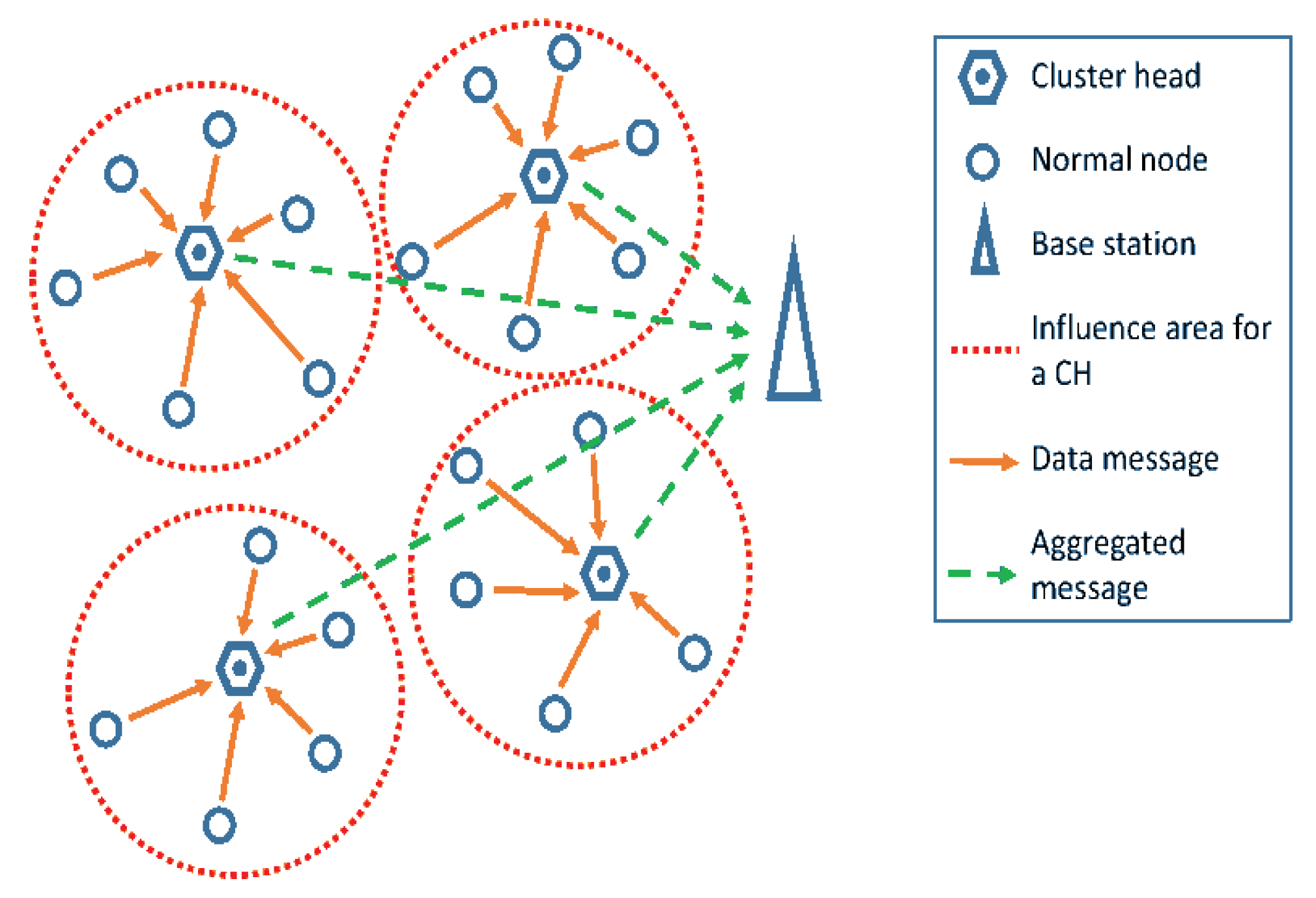
- We went with two-function notations to improve the development of WSNs, i.e., CH using a single fitness function for accountable of data information, sending the data to the base station (BS) in the forwarded node.
- The collection of nodes of all data reach out to the CH and nodes of other members. The collection of CH nodes from the total numbers of nodes are transferred to the base station.
- Battery unit power will rely on the WSN. Operations are deployed to optimize the WSN operations for performance and life-span.
1.5. Research Objective
- Residual power and possibility cost values for the sink and function depend on optimal CH.
- The idea of efficient routing and dependent nodes is to improve performance of the modified gravitational search algorithm (MGSA).
- To increase stronger adaptive multi-objective fuzzy clustering set of rules (EAMOFC) is to optimize the strength intake for multi-objective strong CH choice and improvement in records aggregation.
- Balancing the energy improvement function in developing the energy levels.
1.6. Research Methodlogy
2. Materials and Methods
2.1. GSA—Gravitational Search Algorithm
2.1.1. Position
2.1.2. Effective Gravitation
2.1.3. In Effective Gravitation
2.1.4. Evaluation of Fitness Function
2.2. Single Fitness Function of GSA Algorithm
- The lifetime of a sensor network is broadened, in view of further developed choice of transfer hub and utilization of refreshed GSA.
- Information moving among the sink and CH is improved, despite the fact that CHs are chosen as contingent upon sink closeness to save energy.
- Since hub postponement is an urgent measure for the ideal choice of forwarder hub in MGSA, start to finish, the information transmission time (delay) is reduced.
2.3. Modified Gravitational Search Algorithm—ORS
- (1)
- The selection of cluster heads relies upon the sink distance, likelihood, and leftover energy of hubs. It describes the proposed convention’s presentation.
- (2)
- The inter- and intra-cluster multi-hop station transmission favored the least energy escalated multi-bounce course.
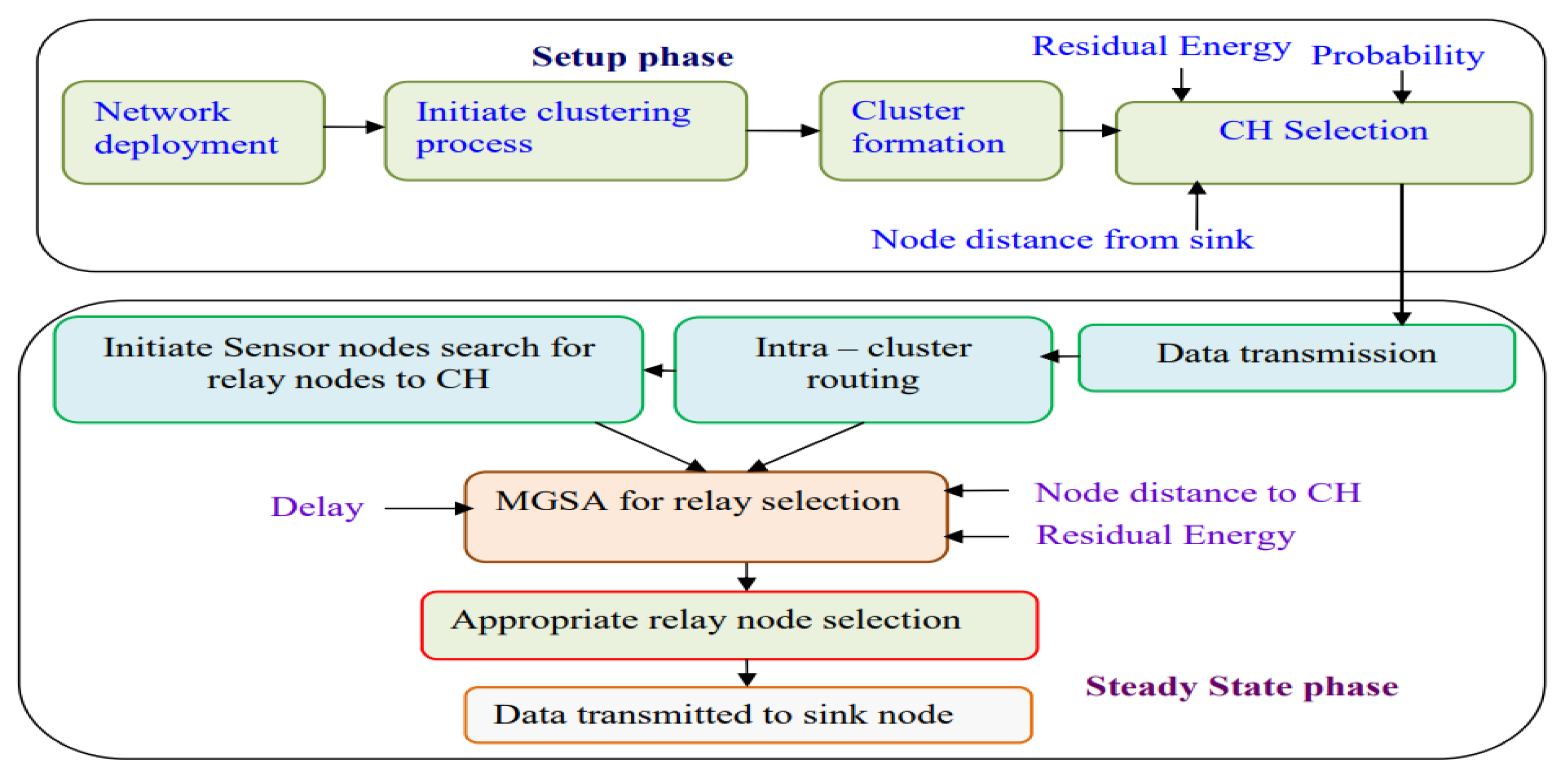
2.4. Cluster Head Selection
| Algorithm 1. Selection of Cluster head |
CH [i] = cluster heads list As the total nodes of Sink(S) = {S1, S2, S3…….Sn} Start: While (CH selection) For cluster node Si Determining the sink distance Compute the sensor node probability Proi Compute(remaining energy) If ((<&& (>&& (> CH [i] = Si; Else End If n connects to CH [i] End |
3. Distance between Nodes to CHs
- xposCH denotes the cluster head’s X-position;
- X-position→XPOSnode is node’s X-position;
- Y-position denotes→yposCH denotes the CH node’s;
- Y-position denotes→yposnode.
4. Delay (D(n))
- Expected transmission count;
- Propagation delay;
- Network’s communication delay.
| Algorithm 2. MGSA for choosing relay node |
| Pi = total particles in WSN |
| fI = particle’s fitness; |
| Bfit =best fitness of the node |
| Eres = residual energy |
| Disti,CH = the proximity, together with sensor nodes and cluster head |
| OFN = relay node or optimal forwarder |
| For ∀ nodes ‘n’ |
| Evaluate f–i of total particles P |
| Calculate Eres |
| Estimate distI,CH |
| Determine Dn |
| End |
| For ∀ nodes ‘n’ |
| OFN = Pi |
| Else |
| End for |
4.1. Derivation of a Cluster Head Selection Fitness Function
- (a)
- Energy: All part hubs impart information to important CH. Bunch head consolidates the approaching information and converts it into a solitary transmission parcel. Later, the bundles are directed to the BS. Therefore, CH utilizes more energy than other sensor hubs. Thus, a sensor hub with most elevated leftover energy should be picked as CH, proposing that energy utilization is lower for low-energy hubs, rather than higher for high-energy hubs. In this way, our underlying object is to limit F1, as we go with the following Equation (8)where Residual Energy = ECHi = Eintinal − Econsumed,
- Eintial → energy of sensor nodes
- Econsumed → consumed energy of sensor nodes
- (b)
- Distance: utilized to decide the typical distance between the BS and sensor hub. It will be brought down when the energy utilization of the CH hubs is at its most minimal. Thus, CH has a more drawn-out life expectancy. The second parameter, F2, can be diminished to Equation (9).where:where:
- xpossink and xposnode—here, the sink and node are denoted;
- ypossink and yposnode tells y position of sink and node.
- (c)
- Probability Value: during CH determination, the sensor hubs make an irregular number. In a few strange occasions, the ‘F1’ and ‘F2’ upsides of at least two sensor hubs might be indistinguishable. In those conditions, the CH’s not set in stone by the likelihood esteem. As an outcome, the third boundary, ‘F3’, can be limited utilizing Equation (10).
| Algorithm 3. Selection of Cluster head |
| Applied excitation: Total sensor nodes set S = (s1, s2, s3 …, sn) Number of agents: Np; dimension K; Response: CHs set Set up the agents Aj, where 1 ≤ j ≤ Np While (j! = Np) do Determine fitness (Aj) End While (j! = Np) do best = max of (fitness(Aj)) worst = min of (fitness(Aj)) End While (j! = Np) do Evaluate mass(Aj) End While (j! = Np) do Find force (Aj), with the help of Equation (3) Evaluate acceleration (Aj), with the help of Equation (4) Updating coordinates CHj with the help of Equations (5) and (6) End Assign sensor to CHs End |
4.2. Derivation of Optimal Relay Selection Fitness Function
- (a)
- Distance between cluster member and CH:
| Algorithm 4. Selection of optimal relay node |
| Applied excitation: Total sensor nodes set S = (s1, s2, s3 …, sn) Number of agents: Np; dimension K; Response: optimal forwarder or relay nodes set Set up the agents Aj, where 1 ≤ j ≤ Np While (j! = Np) do Evaluate fitness (Aj) End While (j! = Np) do best = max of (fitness(Aj)) worst = min of (fitness(Aj)) End While (j! = Np) do Evaluate mass (Aj) End While (j! = Np), do Find force (Aj), with the help of Equation (3) Evaluate acceleration (Aj), with the help of Equation (4) Updating coordinates CHj, with the help of Equations (5) and (6) End Maximum (fitness (A j)) is used to choose forwarder or relay nodes for every route End |
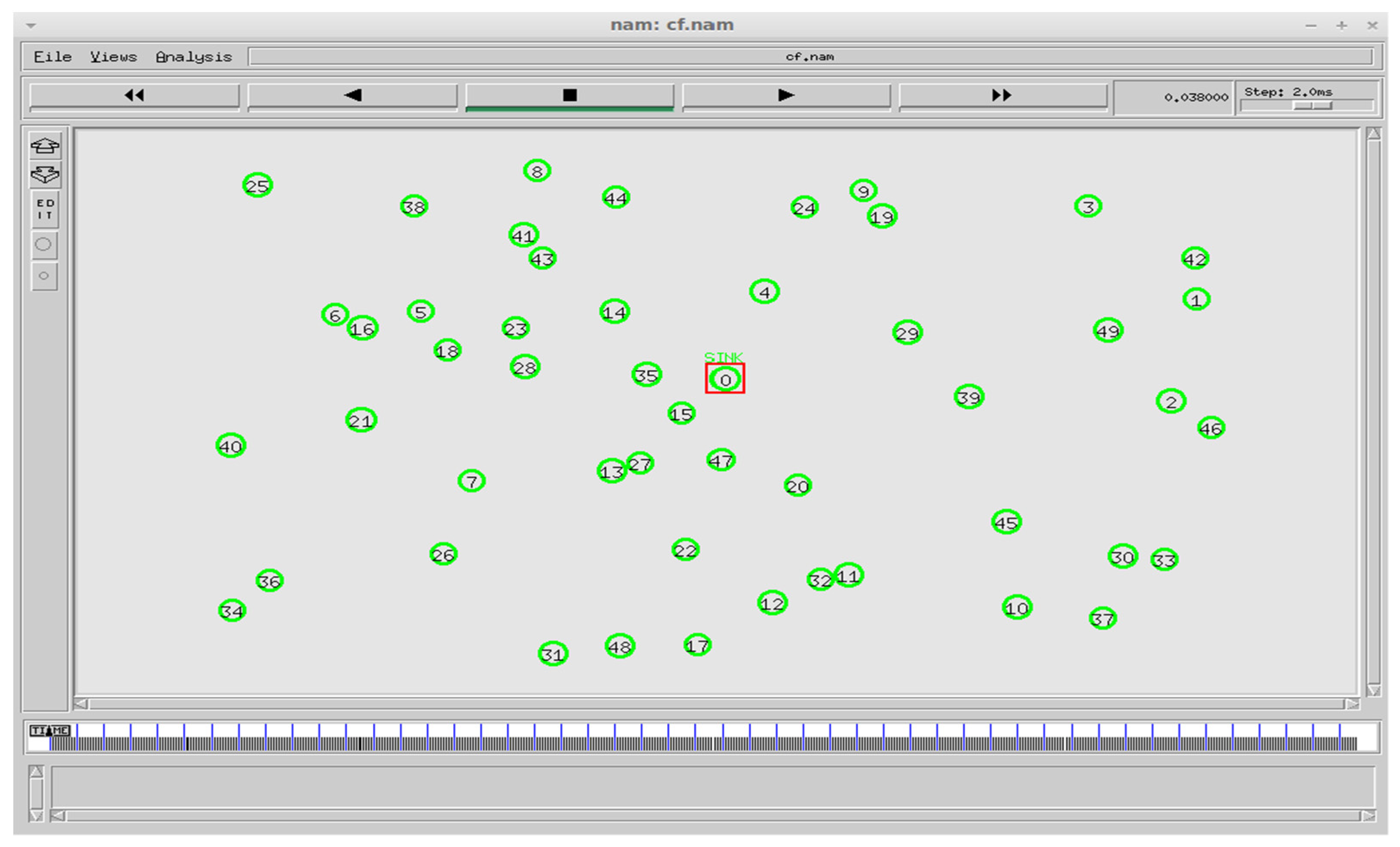
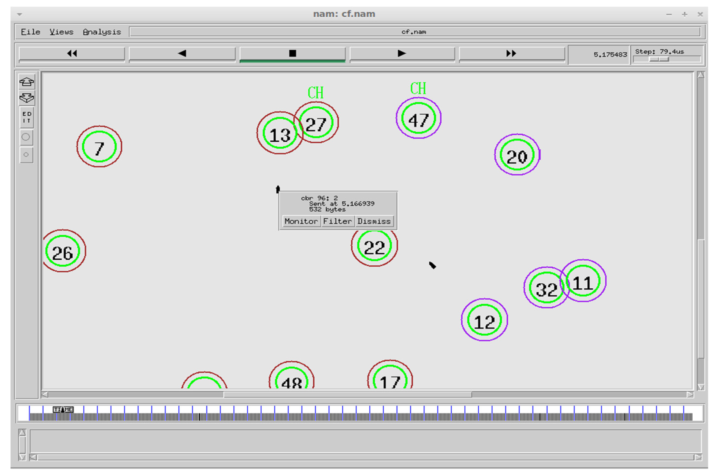
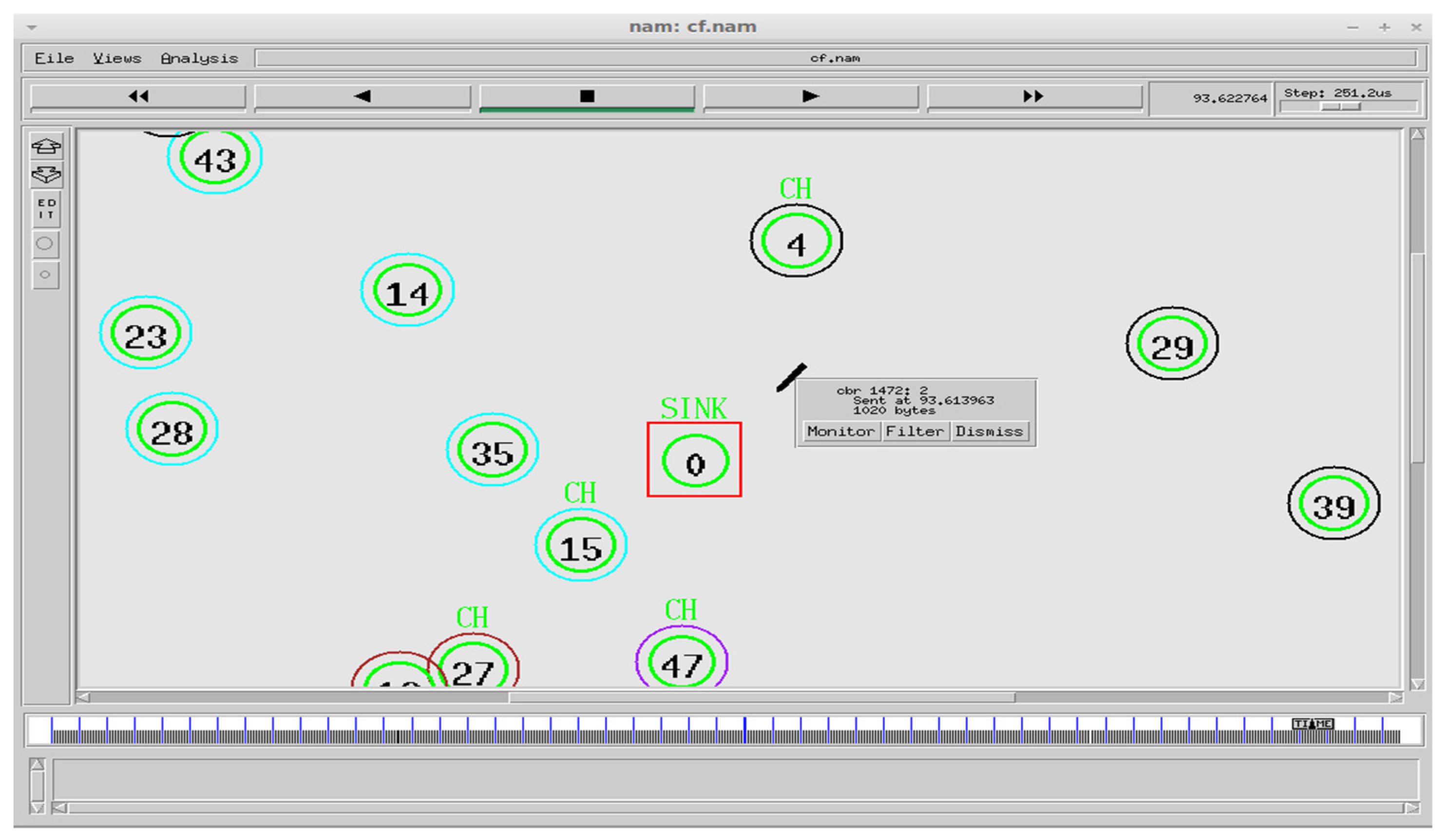
5. Experimental Setup
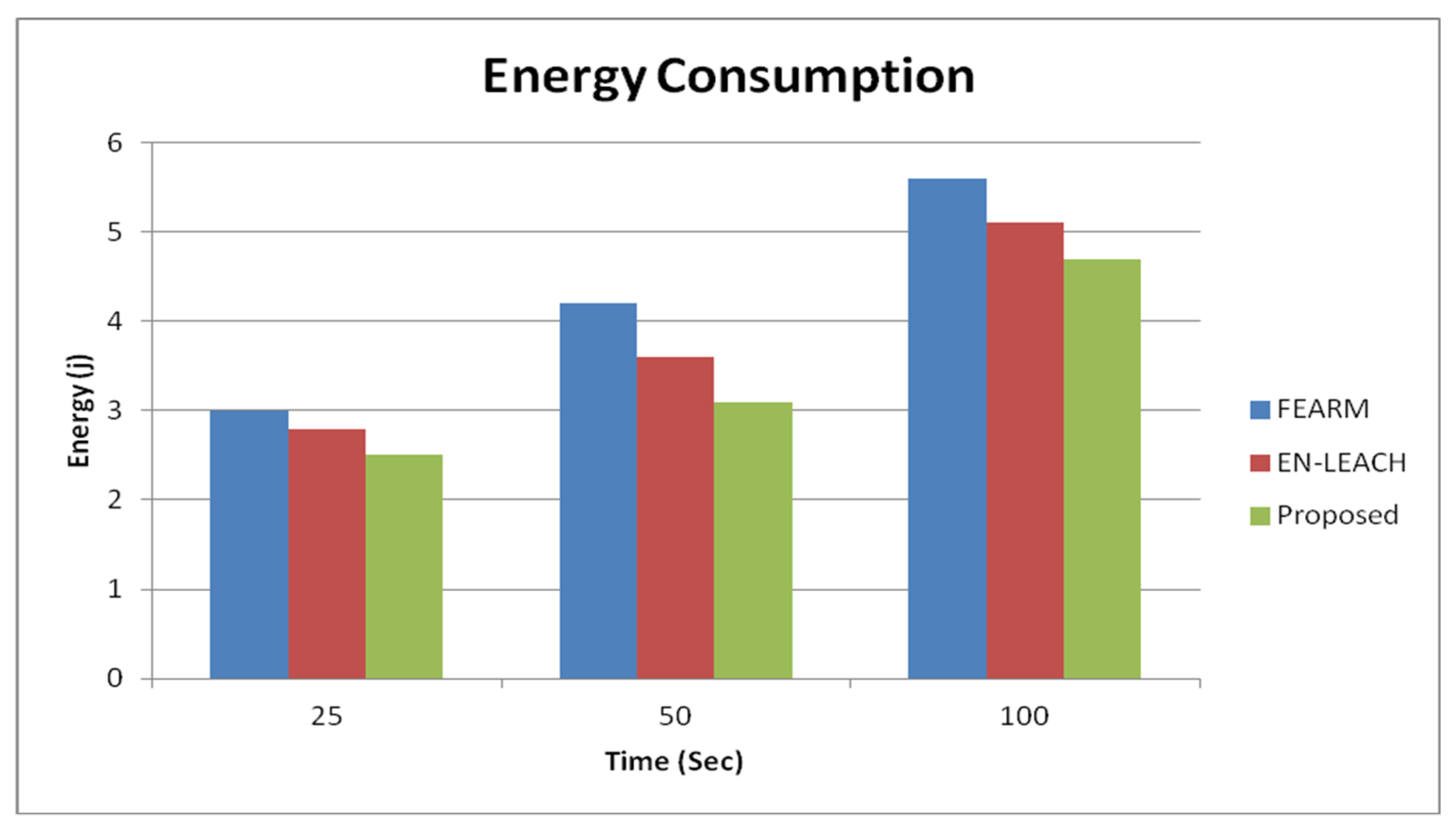
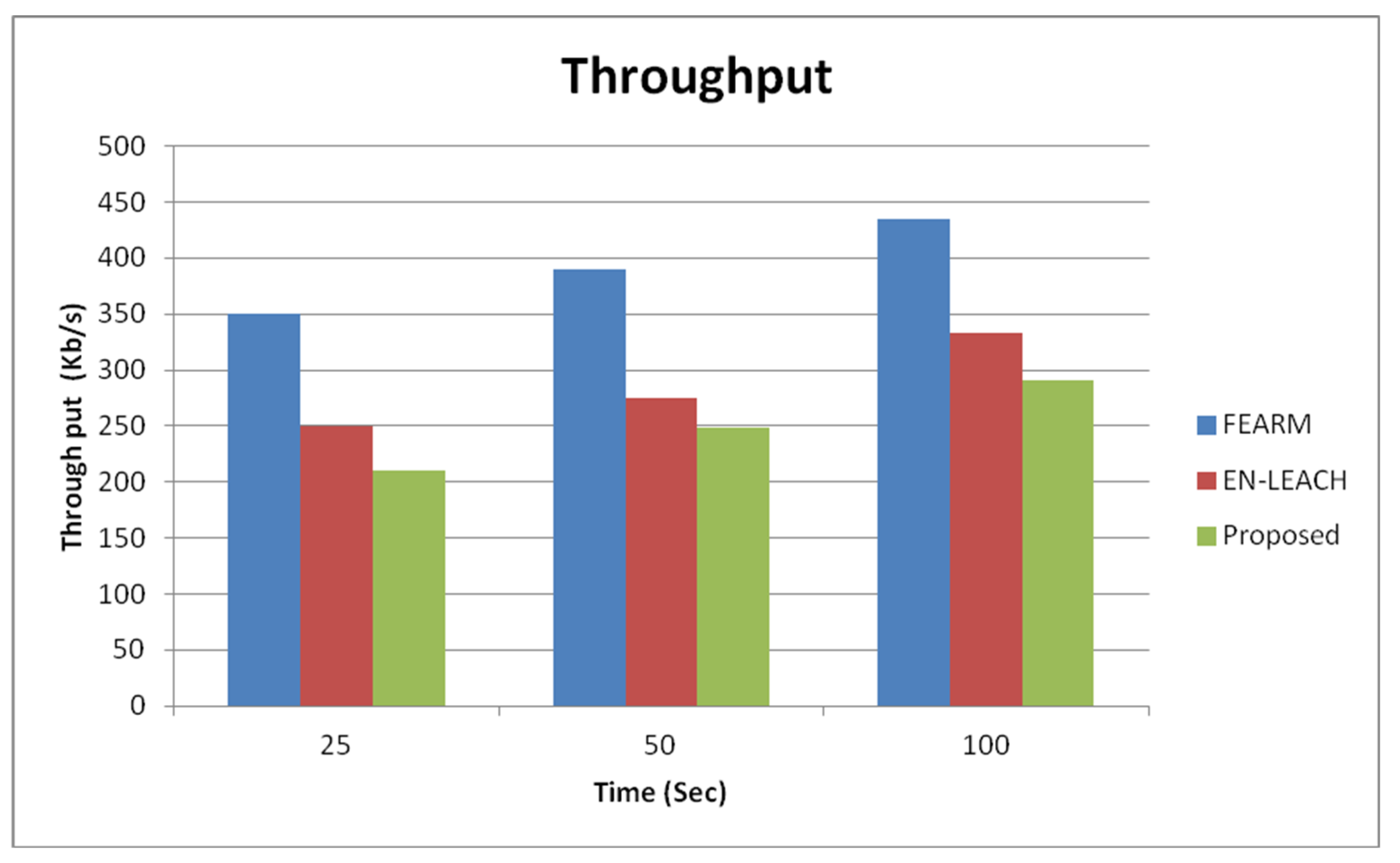
5.1. MGSA—ORS
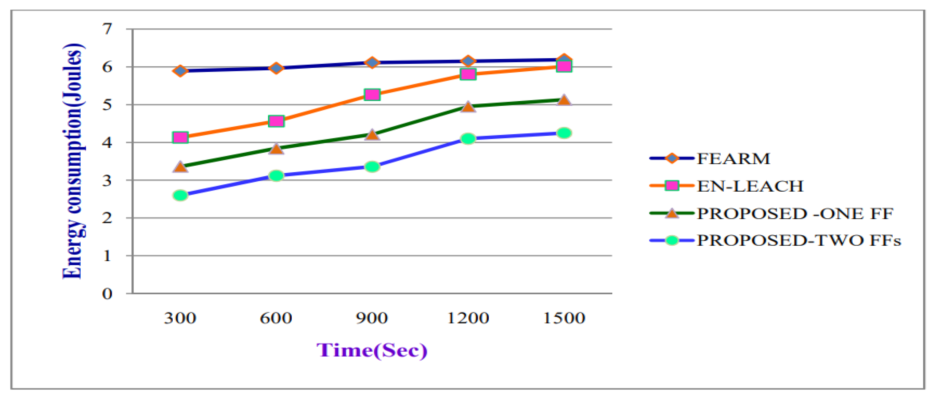
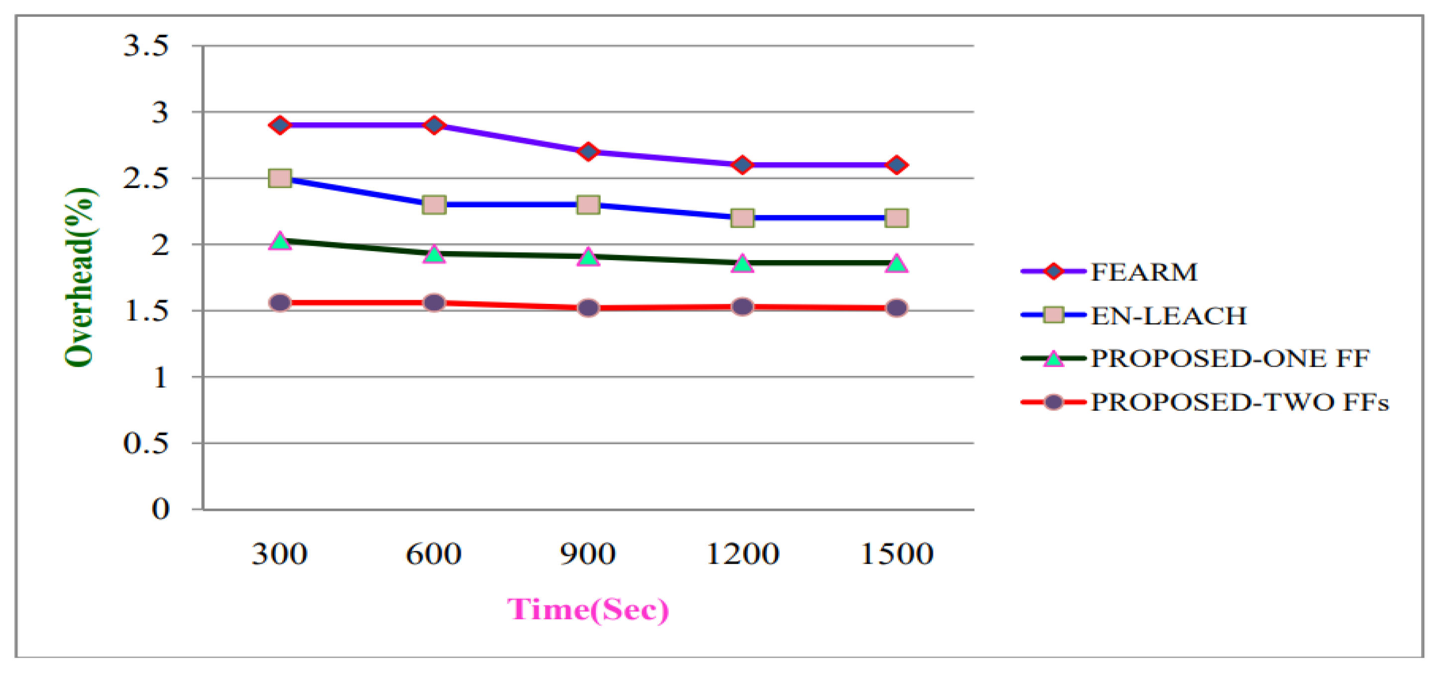
5.2. Modified Gravitational Search Algorithm with Two Fitness Functions
6. Conclusions
Author Contributions
Funding
Institutional Review Board Statement
Informed Consent Statement
Data Availability Statement
Acknowledgments
Conflicts of Interest
Abbreviations
| CH | Cluster head |
| LEACH | Low-energy adaptive clustering hierarchy |
| DMEERP | Dynamic multi-hop energy-efficient routing protocol |
| MMBCR | Min–max battery cost routing |
| CMDR | Conditional minimum drain rate |
| DCFR | Double cost function-based route |
| EAMOFC | Adaptive multi-objective fuzzy clustering |
| RPDR | Received packet delivery ratio |
| Bs | Base station |
| EESRA | Energy efficient scalable routing algorithm |
| MTE | Minimum total energy |
| CMMBCR | Conditional min–max battery cost routing |
| ESCFR | Exponential and sine cost function-based route |
| MGSA | Modified gravitational search algorithm |
| ORS | Optimal relay selection |
| PDR | Packet delivery ratio |
References
- Akyildiz, I.F.; Melodia, T.; Chowdhury, K.R. A survey on wireless multimedia sensor networks. Comput. Netw. 2007, 51, 921–960. [Google Scholar] [CrossRef]
- Akyildiz, I.F.; Kasimoglu, I.H. Wireless sensor and actor networks: Research challenges. Ad Hoc Netw. 2004, 2, 351–367. [Google Scholar] [CrossRef]
- Akyildiz, I.F.; Su, W.; Subramaniam, Y.S.; Cayirci, E. Wireless sensor networks: A survey. Comput. Netw. 2002, 38, 393–422. [Google Scholar] [CrossRef] [Green Version]
- Kashi, S.S.; Sharifi, M. Connectivity weakness impacts on coordination in wireless sensor and actor networks. IEEE Commun. Surv. Tutor. 2013, 15, 145–166. [Google Scholar] [CrossRef]
- Melodia, T.; Pompili, D.; Akyldiz, I.F. Handling mobility in wireless sensor and actor networks. IEEE Trans. Onmobile Comput. 2010, 9, 160–173. [Google Scholar] [CrossRef] [Green Version]
- Mothku, S.K.; Rout, R.R. Adaptive buffering using markov decision process in tree-based wireless sensor and actor networks. Comput. Electr. Eng. 2018, 71, 901–914. [Google Scholar] [CrossRef]
- Zeng, Y.; Li, D.; Vasilakos, A.V. Real-time data report and task execution in wireless sensor and actuator networks using self-aware mobile actuators. Comput. Commun. 2013, 36, 988–997. [Google Scholar] [CrossRef]
- Anwar, A.; Sridharan, D.; Anwar, A.; Sridharan, D. A survey on routing protocols for wireless sensor networks in various environments. Int. J. Comput. Appl. 2015, 112, 13–29. [Google Scholar]
- Akkaya, K.; Younis, M. A Survey on Routing Protocols for Wireless Sensor Networks. Ad Hoc Netw. 2005, 3, 325–349. [Google Scholar] [CrossRef] [Green Version]
- Al-Turjman, F. Hybrid approach for mobile couriers election in smart-cities. In Proceedings of the IEEE Local Computer Networks (LCN), Dubai, United Arab Emirates, 7–10 November 2016; pp. 507–510. [Google Scholar]
- Toldan, P.; Kumar, A.A. Design Issues and various Routing Protocols for Wireless Sensor Networks. In Proceedings of the National Conference on New Horizons in IT, MET, Mumbai, India, 18–19 October 2013; pp. 65–67, ISBN 978-93-82338-79-6. [Google Scholar]
- Abdulqader, M.; Walid, A.; Khaled, A.; Abdulrahman, A. A robust harmony search algorithm based Markov model for node deployment in hybrid wireless sensor network. Int. J. GEOMATE 2016, 11, 2747–2754. [Google Scholar]
- Yick, J.; Mukherjee, B.; Ghosa, D. Wireless sensor network survey. Comput. Netw. 2008, 52, 2292–2330. [Google Scholar] [CrossRef]
- Villalba, L.J.G.; Ana, L.S.O.; Cabrera, A.T.; Abbas, C.J.B. Routing Protocols in Wireless Sensor Networks. Sensors 2009, 9, 8399–8421. [Google Scholar] [CrossRef] [PubMed]
- Heinelman, W.R.; Chandrakasan, A.; Balakrishnan, H. Energy efficient Communication Protocol for Wireless Sensor Networks. In Proceedings of the 33rd Annual Hawaii International Conference on System Sciences, Big Island, HI, USA, 7–10 January 2002; pp. 4–7. [Google Scholar]
- Marjan, R.; Behnam, D.; Kamalrulnizam, A.B.; Lee, M. Multipath Routing in Wireless Sensor Networks: Survey and Research Challenges. Sensors 2012, 1, 650–685. [Google Scholar]
- Tsai, J.; Moors, T. A Review of Multipath Routing Protocols: From Wireless Ad Hoc to Mesh Networks. In Proceedings of the ACoRN Early Career Researcher Workshop on Wireless Multihop Networking, Sydney, Australia, 17–18 July 2006. [Google Scholar]
- Arjunan, S.; Sujatha, P. Lifetime maximization of wireless sensor network using fuzzy based unequal clustering and ACO based routing hybrid protocol. Appl. Intell. 2017, 48, 2229–2246. [Google Scholar] [CrossRef]
- Pantazis, N.A.; Nikolidakis, S.A.; Vergados, D.D. Energy-efficient routing protocols in wireless sensor networks: A survey. IEEE Commun. Surv. Tutor. 2013, 15, 551–591. [Google Scholar] [CrossRef]
- Jakllari, G.; Eidenbenz, S.; Hengartner, N.; Krishnamurthy, S.V.; Faloutsos, M. Link positions matter: A noncommutative routing metric for wireless mesh networks. IEEE Trans. Mob. Comput. 2012, 11, 61–72. [Google Scholar] [CrossRef] [Green Version]
- Liu, X. A typical hierarchical routing Protocols for wireless sensor networks: A review. IEEE Sens. J. 2015, 15, 5372–5383. [Google Scholar] [CrossRef]
- Gherbi, C.; Aliouat, Z.; Benmohammed, M. A survey on clustering routing Protocols in wireless sensor networks. Sens. Rev. 2017, 37, 12–25. [Google Scholar] [CrossRef]
- Mundada, M.R.; Kiran, S.; Khobanna, S.; Varsha, R.N.; George, S.A. A study on energy efficient routing Protocols in wireless sensor networks. Int. J. Distrib. Parallel Syst. 2012, 3, 311–330. [Google Scholar] [CrossRef]
- Ye, W.; Heidemann, J.; Estrin, D. An energy-efficient MAC protocol for wireless sensor networks. In Proceedings of the Twenty First Annual Joint Conference of the IEEE Computer and Communications Societies, New York, NY, USA, 23–27 June 2002; Volume 3. [Google Scholar]
- Zhu, J.; Qiao, C.; Wang, X. On accurate energy consumption models for wireless ad hoc networks. IEEE Trans. Wirel. Commun. 2006, 5, 3077–3086. [Google Scholar] [CrossRef] [Green Version]
- Liu, X. A survey on clustering routing Protocols in wireless sensor networks. Sensors 2012, 12, 11113–11153. [Google Scholar] [CrossRef] [PubMed] [Green Version]
- Kole, S.; Vhatkar, K.; Bag, V. Distance-based cluster formation technique for LEACH protocol in wireless sensor network. Int. J. Appl. Innov. Eng. Manag. 2014, 3, 2319–4847. [Google Scholar]
- Mothku, S.K.; Rout, R.R. Adaptive Fuzzy-Based Energy and Delay-Aware Routing Protocol for a Heterogeneous Sensor Network. J. Comput. Netw. Commun. 2019, 2019, 3237623. [Google Scholar] [CrossRef]
- Sharma, Y.; Bagla, A. Security Challenges for Swam robotics. Secur. Chall. 2009, 2, 45–48. [Google Scholar]
- Salem, A.O.A.; Shudifat, N. Enhanced LEACH protocol for increasing a lifetime of WSNs. Pers. Ubiquitous Comput. 2019, 23, 901–907. [Google Scholar] [CrossRef]
- Sateesh, G.; Bhuvaneswari, M.V.; Sonam, P.; Prakash, M.C.; Alekya, M.G.P.; Mustafa, M. Energy efficient routing in wireless sensor networks using residual energy of nodes. Int. J. Innov. Eng. Technol. 2019, 12, 1–12. [Google Scholar]
- Han, G.; Zhang, L. WPO-EECRP: Energy-efficient clustering routing protocol based on weighting and parameter optimization in WSN. Wirel. Pers. Commun. 2017, 98, 1171–1205. [Google Scholar] [CrossRef]
- Arivubrakan, P.; Sundari, S. A protocol-based routing technique for enhancing the quality of service in multi hop wireless networks. Int. J. Innovat. Technol. Explor. Eng. 2019, 8, 1182–1186. [Google Scholar]
- Elsmany, E.F.A.; Omar, M.A.; Wan, T.C.; Altahir, A.A. EESRA: Energy efficient scalable routing algorithm for wireless sensor networks. IEEE Access 2019, 7, 96974–96983. [Google Scholar] [CrossRef]
- Nivedhitha, V.; Saminathan, A.G.; Thirumurugan, P. DMEERP: A dynamic multi-hop energy efficient routing protocol for WSN. Microprocess. Microsyst. 2020, 79, 103291. [Google Scholar] [CrossRef]
- Rodoplu, V.; Meng, T.H. Minimum energy mobile wireless networks. IEEE J. Sel. Areas Commun. 1999, 17, 1333–1344. [Google Scholar] [CrossRef] [Green Version]
- Singh, S.; Woo, M.; Raghavendra, C.S. Power-aware routing in mobile ad hoc networks. In Proceedings of the 4th annual ACM/IEEE International Conference on Mobile Computing and Networking, Dallas, TX, USA, 25–30 October 1998; pp. 181–190. [Google Scholar]
- Toh, K. Maximum battery life routing to support ubiquitous mobile computing in wireless ad hoc networks. IEEE Commun.Mag. 2001, 39, 138–147. [Google Scholar] [CrossRef] [Green Version]
- Kim, D.; Garcia-Luna-Aceves, J.; Obraczka, K.; Cano, J.-C.; Manzoni, P. Routing mechanisms for mobile ad hoc networks based on the energy drain rate. IEEE Trans. Mob. Comput. 2003, 2, 161–173. [Google Scholar]
- Chang, J.-H.; Tassiulas, L. Maximum lifetime routing in wireless sensor networks. IEEE/ACM Trans. Netw. 2004, 12, 609–619. [Google Scholar] [CrossRef]
- Ok, C.S.; Lee, S.; Mitra, P.; Kumara, S. Distributed energy balanced routing for wireless sensor networks. Comput. Ind. Eng. 2009, 57, 125–135. [Google Scholar] [CrossRef]
- Liu, G.; Ma, M.; Liu, C.; Shu, Y. Adaptive fuzzy multiple attribute decision routing in vanets. Int. J. Commun. Syst. 2017, 30, e3014. [Google Scholar] [CrossRef]
- Taheri, H.; Neamatollahi, P.; Younis, O.M.; Naghibzadeh, S.; Yaghmaee, M.H. An energy-aware distributed clustering protocol in wireless sensor networks using fuzzy logic. Ad Hoc Netw. 2012, 10, 1469–1481. [Google Scholar] [CrossRef]
- Rashedi, E.; Nezamabadi-Pour, H.; Saryazdi, S. BGSA: Binary gravitational search algorithm. Nat. Comput. 2010, 9, 727–745. [Google Scholar] [CrossRef]
- Soleimanpour-Moghadam, M.; Nezamabadi-Pour, H.; Farsangi, M.M. A quantum inspired gravitational search algorithm for numerical function optimization. Inf. Sci. 2014, 267, 83–100. [Google Scholar] [CrossRef]
- Nezamabadi-Pour, H. A quantum-inspired gravitational search algorithm for binary encoded optimization problems. Eng. Appl. Artif. Intell. 2015, 40, 62–75. [Google Scholar] [CrossRef]
- Handy, M.J.; Haase, M.; Timmermann, D. Low energy adaptive clustering hierarchy with deterministic cluster-head selection. In Proceedings of the IEEE 4th International Workshop on Mobile and Wireless Communications Network, Stockholm, Sweden, 9–11 September 2002; pp. 368–372. [Google Scholar]
- Singh, S.K.; Kumar, P.; Singh, J.P. A Survey on Successors of LEACH Protocol. IEEE Access 2017, 5, 4298–4328. [Google Scholar] [CrossRef]
- Jin, Y.; Vural, S.; Moessner, K.; Tafazolli, R. An EnergyEfficient Clustering Solution for Wireless Sensor Networks. IEEE Trans. Wirel. Commun. 2011, 10, 3973–3983. [Google Scholar]
- Kang, S.H.; Nguyen, T. Distance Based Thresholds for Cluster Head Selection in Wireless Sensor Networks. IEEE Commun. Lett. 2012, 16, 1396–1399. [Google Scholar] [CrossRef]


| Authors and Reference | Category | Brief Description | Limitations |
|---|---|---|---|
| S Kole .S [28] | Article survey | The performance of the LEACH protocol was improved, and the network lifetime was increased, according to a study on the distance-based construction of cluster approach. | The cluster head and relay node selection with fitness function for optimal routing was not covered in this paper because it only focused on the distance-based CH selection. |
| Sai Krishna Mothku [29] | Article survey | An investigation was made on the methods used by fuzzy-based energy-aware and delay-intelligent routing to select effective routes. | Higher percentage of inactive nodes. There are fewer communications in the WSN as a result of these inactive nodes. |
| Abu Salem [30] | Article survey | To solve the shortcomings of the LEACH (low energy adaptive clustering hierarchy) protocol, a survey was carried out. Cluster heads should be selected using EN-LEACH approach, taking into account their proximity to the BS and degree of expertise. | This idea did not encompass multi-hop routing and not reacted to the relay of nodes. |
| Authors and Reference | Brief Description | Cluster Head Selection | Limitations |
|---|---|---|---|
| Sateesh [31] | Proposed an efficient directing by choosing legitimate courses, based on the probability values appointed. | Residual energy. | Different boundaries, such as deferral and battery limit, were not considered for bunch head determination; subsequently, it results in wasteful steering. |
| Han and Zhang [32] | An energy-effective bunching system was executed by choosing suitable courses, in light of the distance among BS and CH. | R.E. and node degree. | This article was specific only to the distance-based CH selection and did not cover cluster head and relay node selection with fitness function for optimal routing. |
| Arivubrak an and Sundari [33] | With the procedures of clear to send and request to send, a new multicast directing convention was presented that chooses the data transfer capacity and multi-bounce distance from CH to group individuals (RTS). With the decreased postponement, this convention builds data transmission and parcel conveyance proportion. | --- | Less number of nodes used. |
| Elsmany Eyman F. Ahmed, Omar [34] | The energy-efficient scalable routing algorithm, which is described in this study, is an energy-efficient clustering and hierarchical routing technique (EESRA). The suggested technique seeks to maximise network longevity despite growing network size. To reduce the stress on the cluster heads and randomise the selection of cluster heads, the method utilises a three-layer structure. | The LEACH protocol’s stochastic rotation technique was used. | There is extension for additional likelihood to diminish energy utilization of the organization. |
| V. Nivedhit ha [35] | The dynamic multi-bounce energy-productive directing convention (DMEERP) picks a course founded on the channel limit model, which is carried out on both the transmitter and beneficiary sides. | Residual energy, delay, and bandwidth. | The creators did not consider mixing secure steering with information total methodology. |
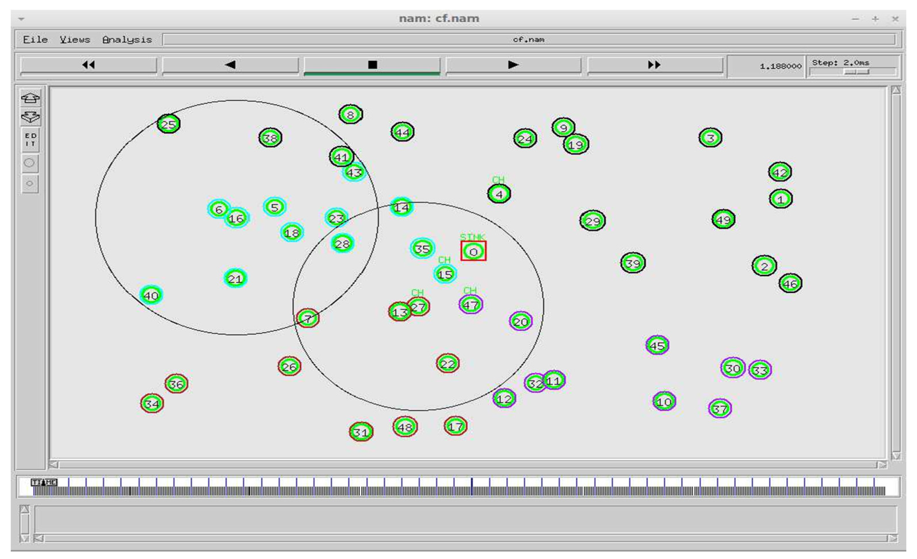
| Cluster No. | Cluster Member Nodes |
|---|---|
| 1 | 7 13 17 22 26 27 31 34 36 48 |
| 2 | 10 11 12 20 30 32 33 37 45 47 |
| 3 | 5 6 14 15 16 18 21 23 28 35 40 43 |
| 4 | 1 2 3 4 8 9 19 24 25 29 38 39 41 42 44 46 49 |
| Sink Node | Node | Node (x_pos, y_pos) | Sink (x_pos,y_pos) | Sink Distance (m) | R.E(J) | Probability |
|---|---|---|---|---|---|---|
| 0 | 7 | (260,223) | (511,344) | 278.64314100 | 99.0325030 | 0.3680650 |
| 0 | 13 | (400,235) | (511,344) | 155.56992000 | 98.9487660 | 0.5082040 |
| 0 | 17 | (484,26) | (511,344) | 319.14416800 | 98.9577950 | 0.9023470 |
| 0 | 22 | (472,142) | (511,344) | 207.69448700 | 98.9097170 | 0.5728850 |
| 0 | 27 | (472,244) | (511,344) | 130.59862200 | 99.8801300 | 0.912580 |
| 0 | 31 | (341,16) | (511,344) | 369.43741000 | 99.0735020 | 0.5851150 |
| 0 | 34 | (25,68) | (511,344) | 558.90249600 | 99.3250840 | 0.2356530 |
| 0 | 36 | (61,103) | (511,344) | 510.47135100 | 99.2608170 | 0.1036330 |
| 0 | 48 | (408,25) | (511,344) | 335.21634800 | 99.0299930 | 0.8960380 |
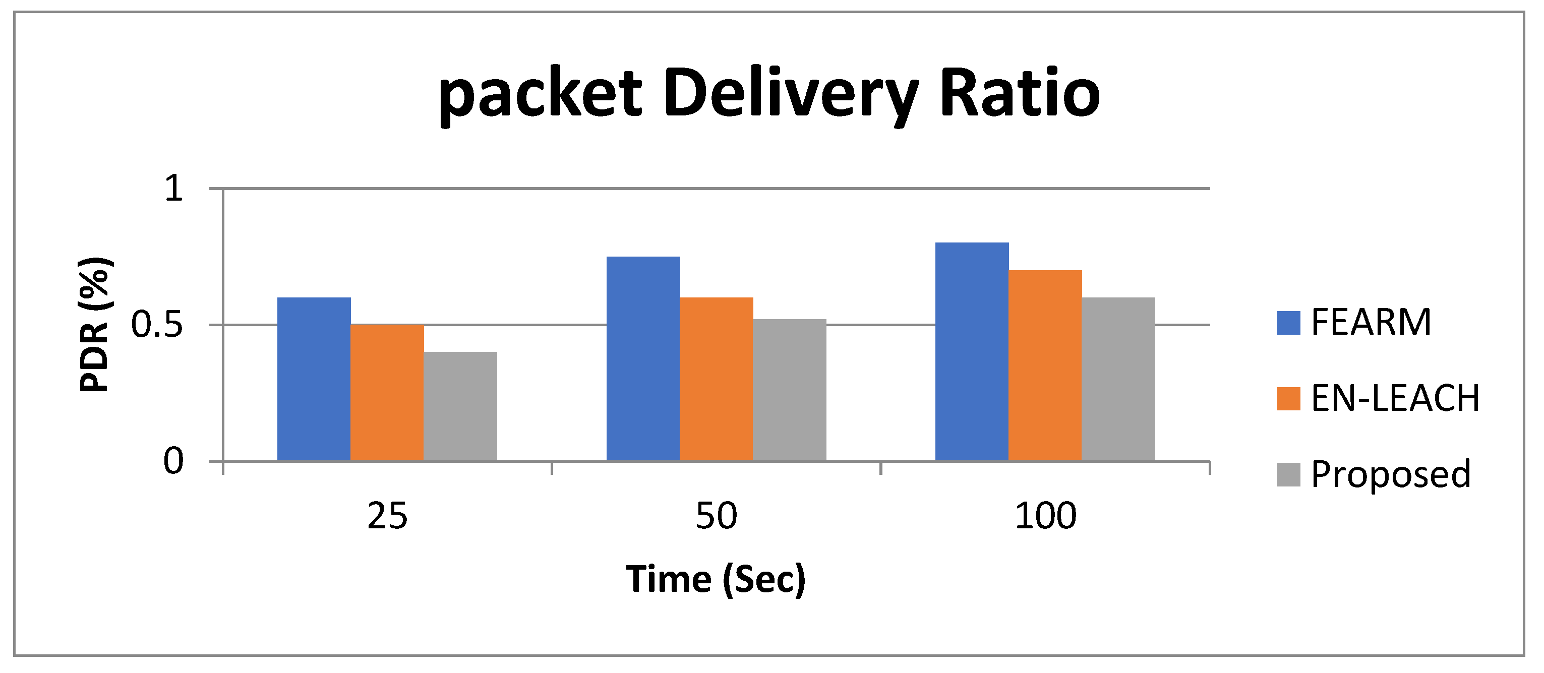
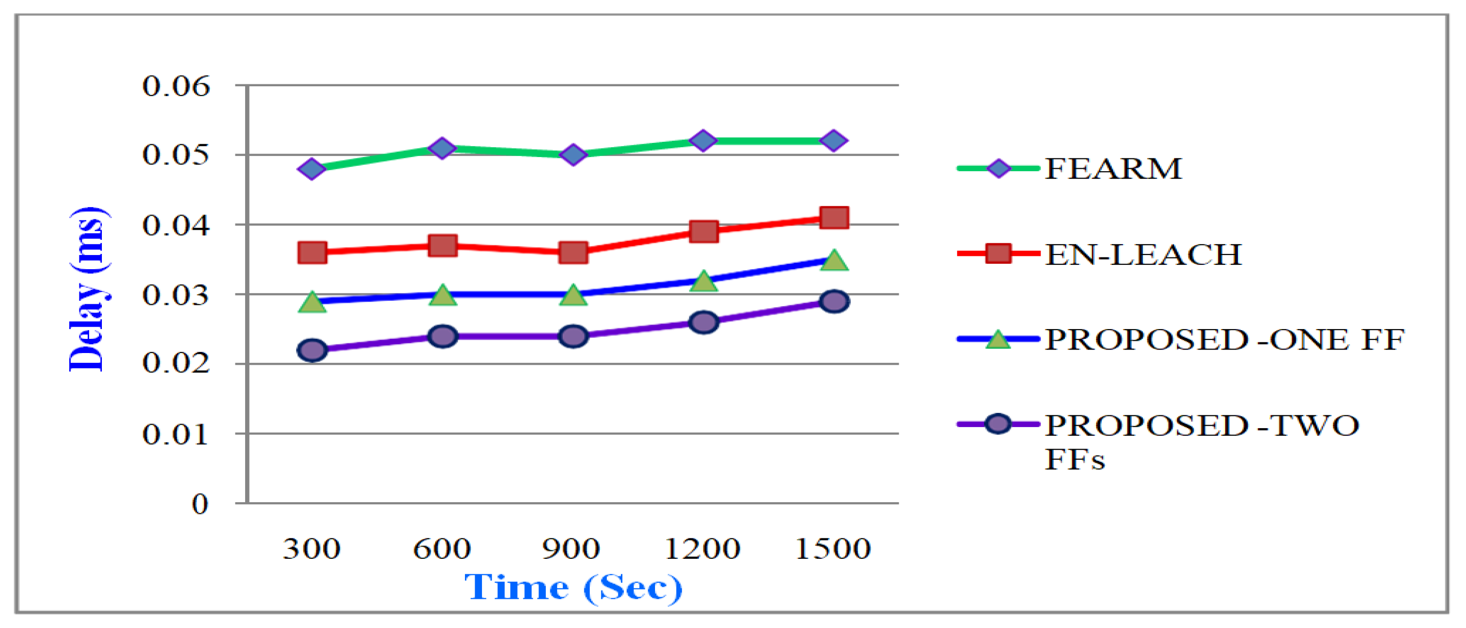
| TIME | FEARM | EN-LEACH | PROPOSED—ONE FF | PROPOSED—TWO FFs |
|---|---|---|---|---|
| 300 | 0.04800 | 0.03600 | 0.02900 | 0.02200 |
| 600 | 0.05100 | 0.03700 | 0.0300 | 0.02400 |
| 900 | 0.0500 | 0.03600 | 0.0300 | 0.02400 |
| 1200 | 0.05200 | 0.03900 | 0.03200 | 0.02600 |
| 1500 | 0.05200 | 0.04100 | 0.03500 | 0.02900 |
| TIME | FEARM | EN-LEACH | PROPOSED—ONE FF | PROPOSED—TWO FFs |
|---|---|---|---|---|
| 300 | 5.8900 | 4.1300 | 3.3600 | 2.600 |
| 600 | 5.9600 | 4.5600 | 3.8400 | 3.1200 |
| 900 | 6.1100 | 5.2600 | 4.2100 | 3.3600 |
| 1200 | 6.1500 | 5.800 | 4.9500 | 4.100 |
| 1500 | 6.1900 | 6.0100 | 5.1300 | 4.2500 |
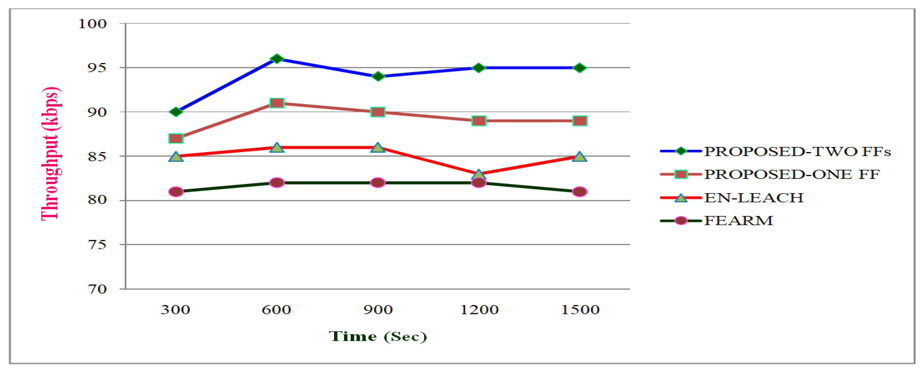
| TIME | FEARM | EN—LEACH | PROPOSED—ONE FF | PROPOSED—TWO FFs |
|---|---|---|---|---|
| 300 | 90.00 | 87.00 | 85.00 | 81.00 |
| 600 | 96.00 | 91.00 | 86.00 | 82.00 |
| 900 | 94.00 | 90.00 | 86.00 | 82.00 |
| 1200 | 95.00 | 89.00 | 83.00 | 82.00 |
| 1500 | 95.00 | 89.00 | 85.00 | 81.00 |
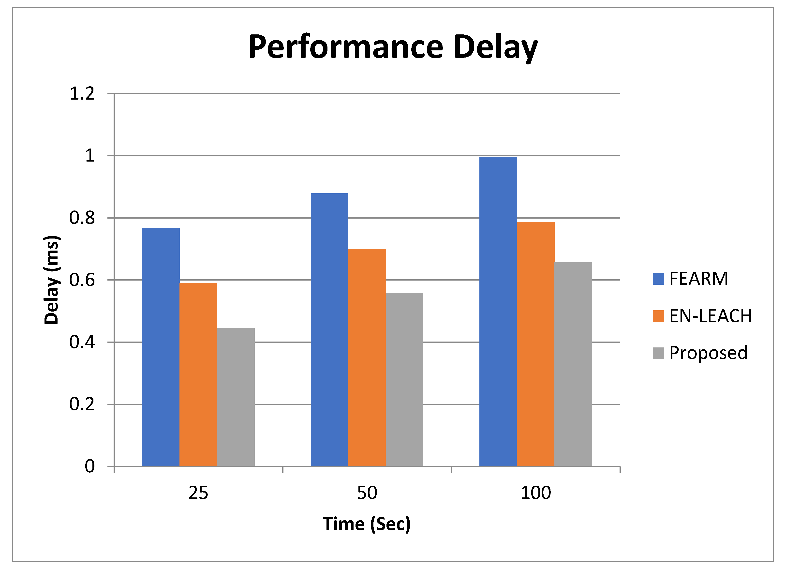
| TIME | FEARM | EN—LEACH | PROPOSED—ONE FF | PROPOSED—TWO FFs |
|---|---|---|---|---|
| 300 | 2.900 | 2.500 | 2.0300 | 1.5600 |
| 600 | 2.900 | 2.300 | 1.9300 | 1.5600 |
| 900 | 2.700 | 2.300 | 1.9100 | 1.5200 |
| 1200 | 2.600 | 2.200 | 1.8600 | 1.5300 |
| 1500 | 2.600 | 2.200 | 1.8600 | 1.5200 |
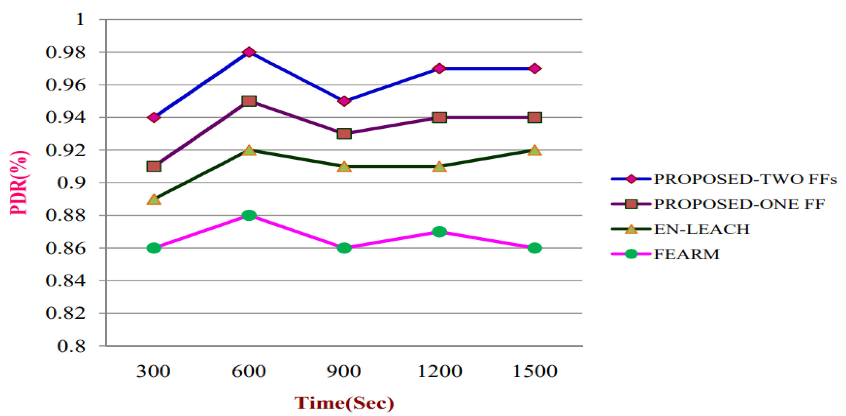
| TIME | FEARM | EN—LEACH | PROPOSED—ONE FF | PROPOSED—TWO FFs |
|---|---|---|---|---|
| 300 | 0.9400 | 0.9100 | 0.8900 | 0.8600 |
| 600 | 0.9800 | 0.9500 | 0.9200 | 0.8800 |
| 900 | 0.9500 | 0.9300 | 0.9100 | 0.8600 |
| 1200 | 0.9700 | 0.9400 | 0.9100 | 0.8700 |
| 1500 | 0.9700 | 0.9400 | 0.9200 | 0.8600 |
Publisher’s Note: MDPI stays neutral with regard to jurisdictional claims in published maps and institutional affiliations. |
© 2022 by the authors. Licensee MDPI, Basel, Switzerland. This article is an open access article distributed under the terms and conditions of the Creative Commons Attribution (CC BY) license (https://creativecommons.org/licenses/by/4.0/).
Share and Cite
Pradeep, S.; Sharma, Y.K.; Verma, C.; Dalal, S.; Prasad, C. Energy Efficient Routing Protocol in Novel Schemes for Performance Evaluation. Appl. Syst. Innov. 2022, 5, 101. https://doi.org/10.3390/asi5050101
Pradeep S, Sharma YK, Verma C, Dalal S, Prasad C. Energy Efficient Routing Protocol in Novel Schemes for Performance Evaluation. Applied System Innovation. 2022; 5(5):101. https://doi.org/10.3390/asi5050101
Chicago/Turabian StylePradeep, S., Yogesh Kumar Sharma, Chaman Verma, Surjeet Dalal, and Cvpr Prasad. 2022. "Energy Efficient Routing Protocol in Novel Schemes for Performance Evaluation" Applied System Innovation 5, no. 5: 101. https://doi.org/10.3390/asi5050101
APA StylePradeep, S., Sharma, Y. K., Verma, C., Dalal, S., & Prasad, C. (2022). Energy Efficient Routing Protocol in Novel Schemes for Performance Evaluation. Applied System Innovation, 5(5), 101. https://doi.org/10.3390/asi5050101