An Improved Model for Analyzing Textual Sentiment Based on a Deep Neural Network Using Multi-Head Attention Mechanism

Abstract

Due to the increasing growth of social media content on websites such as Twitter and Facebook, analyzing textual sentiment has become a challenging task. Therefore, many studies have focused on textual sentiment analysis. Recently, deep learning models, such as convolutional neural networks and long short-term memory, have achieved promising performance in sentiment analysis. These models have proven their ability to cope with the arbitrary length of sequences. However, when they are used in the feature extraction layer, the feature distance is highly dimensional, the text data are sparse, and they assign equal importance to various features. To address these issues, we propose a hybrid model that combines a deep neural network with a multi-head attention mechanism (DNN–MHAT). In the DNN–MHAT model, we first design an improved deep neural network to capture the text’s actual context and extract the local features of position invariants by combining recurrent bidirectional long short-term memory units (Bi-LSTM) with a convolutional neural network (CNN). Second, we present a multi-head attention mechanism to capture the words in the text that are significantly related to long space and encoding dependencies, which adds a different focus to the information outputted from the hidden layers of BiLSTM. Finally, a global average pooling is applied for transforming the vector into a high-level sentiment representation to avoid model overfitting, and a sigmoid classifier is applied to carry out the sentiment polarity classification of texts. The DNN–MHAT model is tested on four reviews and two Twitter datasets. The results of the experiments illustrate the effectiveness of the DNN–MHAT model, which achieved excellent performance compared to the state-of-the-art baseline methods based on short tweets and long reviews.

1. Introduction

Sentiment analysis (SA) of text aims to extract and analyze knowledge from the personal information posted on the internet. Due to its wide range of industrial and academic applications, as well as the increasing growth of social networks, SA has become a hot topic in the field of natural language processing (NLP) in recent years [1]. Thus, different tools and techniques have been proposed to identify the polarity of documents. Polarity detection is a binary categorization task that plays a significant role in most SA applications [2]. Most of the previous approaches for SA have trained shallow techniques on carefully developed efficient features for obtaining satisfactory polarity categorization performances [3]. These models occasionally apply traditional classification approaches involving Naïve Bayes, support vector machines (SVM), and latent Dirichlet allocation (LDA) to linguistic properties, such as lexical features, part-of-speech (POS) tags, and n-grams. However, these approaches have two major drawbacks: (1) the feature distance on which the model must be trained is highly dimensional and scattered and thus affects the model performance; (2) the feature engineering operation is time intensive and an uphill task.

Several current works have suggested learning word embedding [4,5,6] to tackle the above limitations. Word embedding is a dense real-valued vector generated by a neural language model that considers various lexical associations [4,5]. Thus, this makes the employment of word embedding as the input of deep neural networks (DNN) highly common in existing NLP works [4]. In recent years, DNNs have gained increasing attention from many researchers in varied domains, such as medical informatics [6], finance [7], computer vision [8], and multimedia sentiment analysis [9].

DNNs have been suggested for analyzing text data that primarily focus on the performance of machine learning tasks or learning word embedding, such as categorization and clustering. Among the wide range of deep networks, recurrent neural networks (RNNs) and convolutional neural networks (CNNs) are more popular in research related to text processing [10]. The cause of this popularity is due to the fact that the CNN models can learn the local patterns, while the power of RNNs is demonstrated in sequential modelling. Although RNNs are used in several text processing applications, they cannot handle vanishing and exploding gradients, especially if the input data have long dependencies [4]. These dependencies are highly popular in most NLP approaches, especially in the domain of SA.

To deal with the above problem, long short-term memory (LSTM) was introduced [11], which has the ability to capture long dependencies. Due to the potential of LSTM to address the problems of RNNs, it has attracted the attention of many researchers in the field of NLP [12]. Considering both the previous and subsequent contexts, the bidirectional LSTM (Bi-LSTM) model was proposed to combine the forward hidden layers and backward hidden layers. This model can cope with the sequential modelling issue. Bi-LSTM is widely employed in many NLP applications. However, there are two major drawbacks to this model: (1) the high-dimensional input distance popular in the applications of text processing makes the model more complex and thus difficult to improve; (2) the model cannot focus on the significant parts of the context information of the text. To tackle these problems, many studies in the literature have been suggested. For instance, CNNs have been employed to extract meaningful patterns from text and reduce the dimensional feature distance [12]. The attention mechanism assigns various weights for focusing on the significant parts of context [4].

The current deep learning models for SA occasionally handle a few issues and disregard others. For instance, Chatterjee et al. [13] used LSTM and two pre-trained word embeddings for extracting both semantics and sentiments for feeling recognition, but did not address the differences between the importance of various parts of sentences. A study by Liu et al. [14] combined Bi-LSTM with CNN and the benefited attention mechanism, but this study did not consider the co-occurrence of long and short dependencies. Rezaeinia et al. [15] used CNNs and improved pre-trained word embeddings, but they did not take account of the different importance values of words and long dependencies.

The Google machine translation team presented a new concept of multi-head attention mechanism MHAT in 2017 to capture related information in various sub-distances via multiple distributed computations [16]. In our study, we employed the attention mechanism to select the most important contextual information, considered both forward and backward context dependencies, and assigned approximate attention to various words in comments.

In this work, we propose a new deep learning model that combines a deep neural network with a multi-head attention mechanism (DNN–MHAT) for classifying textual sentiment. We first applied a global vector for word representation (GloVe) [5] to create word vectors automatically as the weights in the embedding layer. We also designed an improved deep neural network to capture the text’s actual context and extract the local features of position invariants by combining recurrent Bi-LSTM memory units with a CNN. Then, we devised a multi-head attention mechanism to capture the words in the text that are significantly related to long space and encoding dependencies, which adds effective weights to the different contextual features. Finally, the global average pooling layer was applied to obtain a multi-level pattern representation of the text sequences. A Softmax classifier was applied for classifying the processed context information. The DNN–MHAT model was tested on four reviews and two Twitter datasets. The results of the experiments illustrate the effectiveness of the DNN–MHAT model, which achieved excellent performance compared to the state-of-the-art baseline methods based on short tweets and long reviews. The experiments compared the DNN–MHAT model with five state-of-the-art DNN baseline methods based on SA and text classification datasets. DNN–MHAT outperformed the other five methods in terms of popular performance standards in NLP and the domains of SA. Our contributions are summarized as follows:

• We propose a new deep learning model, namely, DNN–MHAT, for text classification and SA tasks. First, we design an improved deep neural network to capture the text’s actual context and extract the local features of position invariants using Bi-LSTM and CNN. Then, we present a multi-head attention mechanism to capture the words in the text that are significantly related to long space and encoding dependencies, assigning weighted importance to different information, efficiently enhancing the sentiment polarity of words and detecting the significant information in the text.
• We investigate the effectiveness of the DNN–MHAT model on two types of datasets: long reviews and short tweets on social media. Compared to five existing deep structures, the DNN–MHAT achieved better performance on two types of datasets.

The rest of this paper is structured as follows: Section 2 contains the Literature Review. Section 3 contains the Materials and Methods. Section 4 contains Experiments and Results. Finally, Section 5 contains the Conclusions and Future Work.

2. Literature Review

2.1. Sentiment Analysis

Most traditional SA research works have utilized supervised machine learning approaches as their clustering module or main classification [17]. These approaches exploited n-gram features and bag-of-words (BOW) techniques to classify and present user-created texts that bear sentiment [18]. These features are presented to cope with the issues of simple BOW techniques, such as overlooking the order of the word and the syntactic structures [19]. The major drawback of utilizing n-gram features, especially when n ≥ 3, is that the result of the feature space is highly dimensional. To handle this drawback, feature selection techniques have been widely applied in recent studies [20,21].

SVM, Naïve Bayes (NB) and artificial neural networks (ANN) are among the common methods employed to extract the meanings of users from their text, and have achieved good performance [22,23,24]. One of the problems that the supervised methods suffer from is that they are sometimes slow and require a large amount of time during training. To solve these problems, many methods based on unsupervised lexicons have been proposed [18,25]. These approaches are scalable, fast, and simple. However, they significantly rely on the lexicon, making them less accurate than their supervised counterparts [25,26]. Field dependency is another issue of lexicon-based approaches, making them less applicable for fields that do not contain specific lexicons.

Due to the advantages of both lexicon- and supervised-based methods, few researchers have taken these advantages and then combined them in various ways [27,28]. For instance, for SA, Zhang et al. [29] proposed a method that consists of two steps for the entity level of tweets. The first step is a high recall based on the supervised method. The second step is a high precision based on the lexicon method. A hybrid model for concept-based sentiment analysis combines machine learning methods and lexicon-based proposed by Mudians et al. [30]. Their method provided a more accurate and justified explanation than purely statistical methods and outperformed lexicon-based methods in detecting the strength of sentiment and polarity.

2.2. DNN for Sentiment Analysis

In the sentiment analysis domain, most existing DNN-based works have been oriented towards learning word embedding or exploiting various types of DNNs for clustering or classification tasks. Word embeddings are generated for capturing word similarities and lexical relationships [31]. Unsupervised methods are usually used to generate such embeddings. These methods are generated according to words with similar contexts and meanings, so they must have similar vectors. The drawback of this supposition is that the vectors of some words are similar, especially those occurring in a small neighborhood, but they are linguistically different. For instance, some words that carry feelings and have the opposite meaning (e.g., bad and good) have similar vectors since they sometimes co-occur in similar contexts. To cope with this problem, few studies have suggested sentiment-aware word vectors generated based on supervised approaches and large sentiment lexicons [4,32,33,34]. A study by Petrucci and Dragoni [35] suggested a new neural word embedding approach for multi-field SA. The authors solvedthe major limitations of former approaches, which did not perform well when used in different fields from the one they were trained on. Their new approach performed better.

In SA applications, the LSTM and its variants [36] are widely utilized due to their ability to handle long-term dependencies. For instance, a novel model using LSTM and a recurrent neural network called P-LSTM was suggested by Chi Lu et al. [37]. The P-LSTM model used three-word phrase embedding rather than single word embedding. To extract accurate data from the text, the P-LSTM model presented the factor mechanism of the phrase that combines the feature vectors of the phrase embed layer and the hidden layer of LSTM. Ju et al. [38] presented a Cached LSTM model (CLSTM) that captured the semantic information of long texts. In recent years, Chatterjee et al. [13] introduced a multi-channel LSTM called SS-BED to detect sentiments in tweets. In the SS-BED model, Sentiment-Specific Word Embedding (SSWE) [39] and GloVe are employed in parallel for pre-trained word embedding. Three LSTM models are implemented sequentially for handling the long dependencies of texts. Finally, the two outputs of the feature vectors are sequenced as inputs in the fully connected layer. The SS-BED model does not address the differences in the importance of various parts of sentences.

CNNs are applied in applications of SA for extracting local features. These models are beneficial when the text is long and specific local features, such as n-grams, are significant. For instance, Rezaeinia et al. proposed a model based on CNN, which availed optimized word embedding to analyze the sentiment at the document level [15]. Their model optimized pre-trained GloVe and Word2Vec embedding [40] with positional, syntactical, and lexical features, but this study did not consider the different importance of words and long dependencies.

In recent years, the attention mechanism has been applied to optimize models of DNNs by allowing them to identify where to concentrate for learning. For instance, for binary sentiment classification, one BiLSTM layer and a global pooling mechanism model were suggested by Zabit et al. [14]. For text classification and question answering, Liu and Guo [41] proposed a hybrid model that combines Bi-LSTM, CNN and the attention mechanism, AC-BiLSTM. Their model used a one-dimensional CNN layer on the word embedding layer to extract local features, BiLSTM for extracting long dependencies, and an attention mechanism for focusing on significant text domains. The AC-BiLSTM model did not consider the co-occurrence of both long and short dependencies. Zhou et al. proposed a BiLSTM model with an attention mechanism to identify the significant features [42]. For text classification, a new attention model-based network called the hierarchical attention network (HAN) was proposed by Yang et al. [43]. The HAN model utilized two attention models at the sentence and words levels. They stacked the attention models on the outputs of gated recurrent unit GRU-based sequence encoders. The Google machine translation team presented a new concept of MHAT in 2017 [16] to capture related information in various sub-distances via multiple distributed computations.

Recently, few researchers have proposed hybrid DNNs for SA. For instance, Mohammad et al. [44] suggested an attention-based bidirectional CNN-RNN deep model for sentiment analysis (ABCDM), which combines an attention mechanism and a bidirectional CNN–RNN deep model. This model first uses GloVe embedding as the weights to the embedding layer, then two bidirectional GRU and LSTM layers for extracting past and future contexts and an attention mechanism for focusing on different words. Convolution and pooling mechanisms are applied to extract local features static position and reduce feature dimensions. A study that combines CNN and GRU with an attention mechanism, named ARC, proposed by Wen and Li [45] to classify reviews and tweets. They employed three various CNN modules for extracting local n-gram and global patterns and bidirectional GRU units. However, these models do not accurately determine the various degrees of importance of forward and backward directions.

The major difference between our model and the DNN baseline models is that our proposed model considers the following significant features simultaneously: (i) short and long context dependencies utilizing Bi-LSTM; (ii) identifying most significant features strong to positional changes utilizing CNNs with various kernels, filter sizes, and pooling mechanisms; (iii) capturing the words in the text that are significantly related to long space and encoding dependencies utilizing a multi-head attention mechanism.

3. Materials and Methods

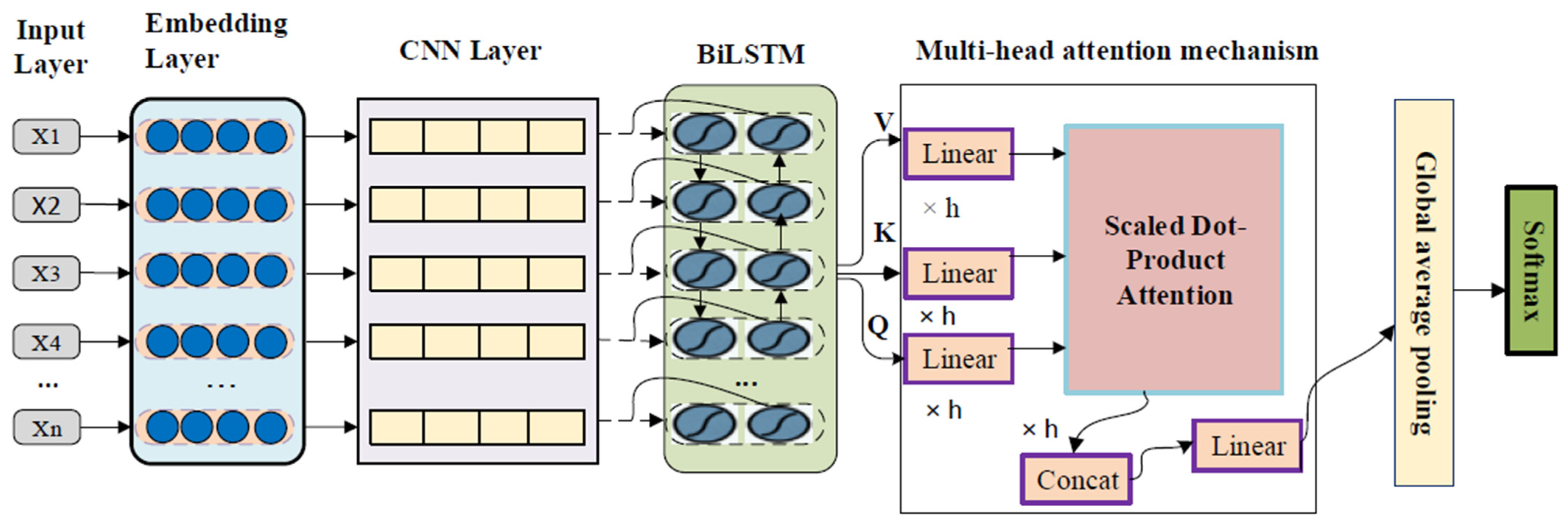
This section describes the overall structure of the DNN–MHAT model, which comprises six fundamental components: the input layer, convolutional neural network, long short-term memory, global average pooling layer, multi-head attention mechanism, and Softmax layer. The overall structure of the DNN–MHAT model is shown in Figure 1. The key goal of the DNN–MHAT model is to detect the polarity of sentiment for the given sentences.

In our method, first, we preprocessed the input data by tokenizing the input text, removing stop words, and dealing with the capitalization of words. Then, the tokenized texts were fed into the word embedding module. After that, the obtained word embedding vectors were fed into a CNN layer. The output of the CNN layer was fed into a Bi-LSTM layer. The output of the Bi-LSTM layer was fed into a multi-head attention module. After that, a global average pooling was applied to obtain the final representation. Finally, the final representation was fed into the Softmax classifier layer. Figure 2 shows the flowchart of the DNN–MHAT model.

3.1. Input Layer

A pre-trained GloVe embedding matrix was utilized to create the input comment matrix $W_g \in R^{n\times e}$ where $e$and $n$refer to the embedding dimension and the total number of words, respectively. For embedding a comment vector, $c \in R^m , m$represents the maximum number of words $w_t$ or the padding length, $t \in \left[1,m\right]$deemed in the comment as shown below:

$$w_t=W_g{w}_t, t\in \left[1,m\right]$$

(1)

3.2. Convolutional Neural Network

CNNs contain many convolution layers employed in the applications of NLP for extracting local features. In CNNs, linear filters are used to perform the convolution process on the features of the input data. Initially, an embedding vector of size $e$ is generated to apply the CNN to a sentence $S$ containing a set of $s$words. Then, the filter $f$ of the size $e\times h$is frequently used in sub-matrices as the input feature matrix. The results in a feature map $M=m_0, m_1, \dots , m_{s-h}$are shown below:

$$m_i=f·S_{i:j+h-1}$$

(2)

where $i=0,1,2,\dots , s-h$ and $S_{i:j}$ represent a sub-matrix of $S$from row i to $j$. The sub-sampling layer or pooling layer is a popular practice in which feature maps are fed to reduce dimensions. Max-pooling is a common pooling strategy that determines the essential feature $b$ of the feature map, as shown in the following equation:

$$b=\underset{0\le i\le s-h}{\max } \{m_i\}$$

(3)

The outputs of the pooling layer are used as the input to the fully connected layer, where these outputs are a pooled feature vector or concatenated (see Figure 1).

3.3. Long Short-Term Memory

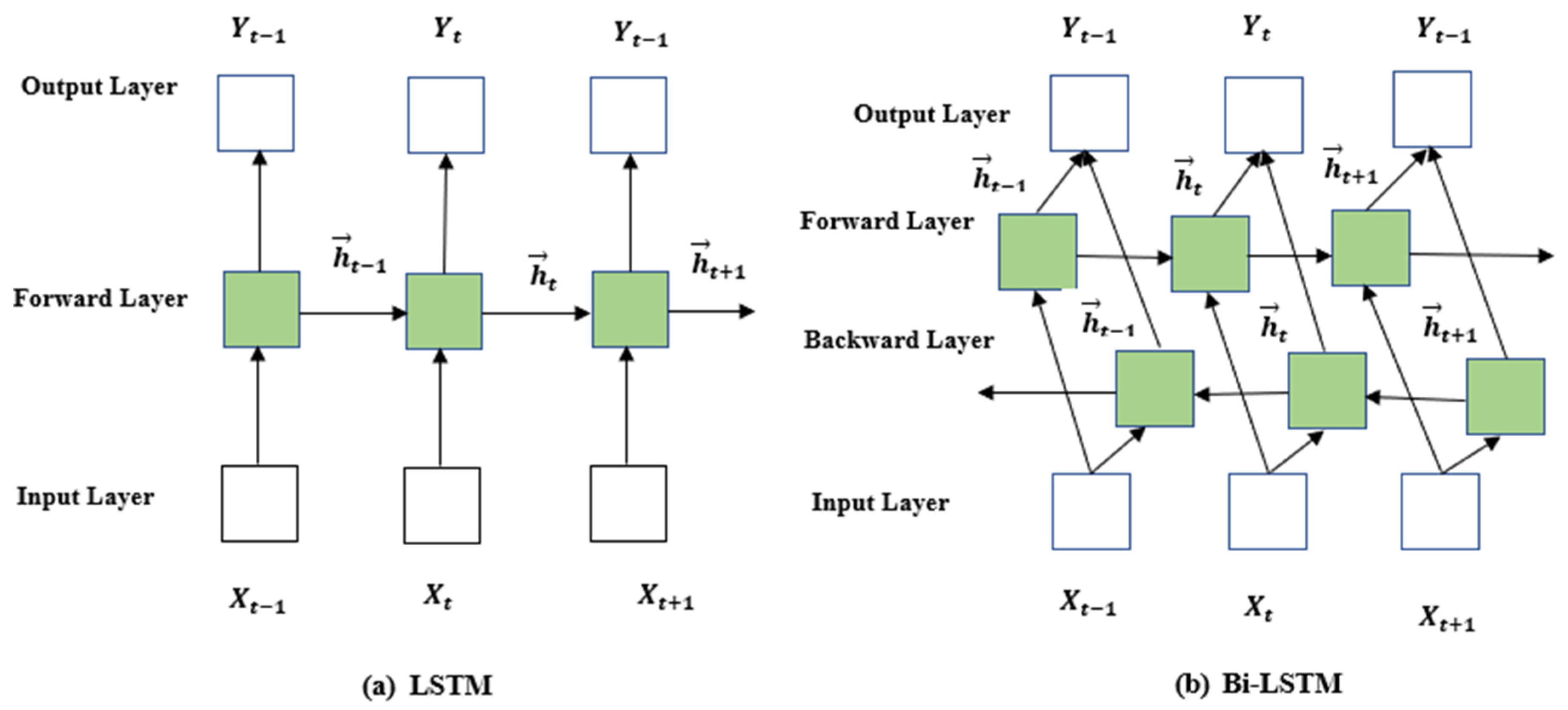
RNNs are a type of feed-forward neural network. RNNs possess a recurrent hidden state activated by using the previous states and can deal with the variable-length sequences and automatically model the contextual information. LSTM is an improved type of RNN (see Figure 3a) designed to solve the exploding/vanishing issues faced by RNNs. The LSTM model contains a chain of recurrent memory units, and each of these chains implicates three “gates” with various functions. An LSTM unit contains three gates: input gate $i_t$, forget gate $f_t$, and output gate $o_t,$ and memory cell $c_t$ to maintain its state over random time intervals. These gates have been generated to organize the flow of data entering and leaving the memory cell. Suppose tanh (.), σ(.), and ⊙ are the hyperbolic tangent function, the sigmoid function and product, respectively. $h_t$is the hidden state vector at time$t$, and $x_t$is the input vector at time$t$. $W$and $U$illustrate cells for input $x_t$or the weight matrices of gates. The hidden state $h_t$and $b$indicate the bias vectors. In the forget gate $f_t$, it defines what information to ignore from the cell state, as indicated by the following equation [41]:

$$f_t=\sigma \left(W_f{h}_{t-1}+U_f{x}_t+b_f\right)$$

(4)

The input gate $i_t$ defines what must be stored by calculating $\widetilde{c_t} \mathrm{and}$ $i_t$ and combining them based on the following equations [41]:

$$i_t=\sigma \left(W_i{h}_{t-1}+U_i{x}_t+b_i\right)$$

(5)

$$\widetilde{c_t}=\tanh \left(W_c{h}_{t-1}+U_c{x}_t+b_c\right)$$

(6)

$$c_t=f_t \odot c_{t-1}+i_t \odot +\widetilde{c_t}$$

(7)

The output gate $o_t$ defines what information is outputted according to the state of the cell state based on the following equations [41]:

$$o_t=\sigma \left(W_o{h}_{t-1}+U_o{x}_t+b_o\right)$$

(8)

$$h_t=o_t \odot \tanh \left(c_t\right)$$

(9)

The LSTM model is based on serial information, but it is not beneficial, especially if you can reach the following information based on the previous model. Therefore, this is highly useful for sequencing tasks.

The Bi-LSTM model comprises a forward ${\overrightarrow{h}}_t$ and a backward ${\overleftarrow{h}}_t$LSTM layer (see Figure 3b). The core goal of the Bi-LSTM structure is that the forward layer ${\overrightarrow{h}}_t$ captures the previous sequential information, and the backward ${\overleftarrow{h}}_t$ captures the subsequent sequential information; both layers are connected to the same output layer. The most important feature of the BiLSTM architecture is that sequence contextual information is considered. Suppose that the input of time $t$is the word embedding $w_t$, at time $t-1$, the output of the forward layer is${\overrightarrow{h}}_{t-1}$ and the output of the forward hidden layer and the backward hidden layer is ${\overrightarrow{h}}_{t-1}$, ${\overleftarrow{h}}_{t+1}$, respectively. The output of the backward and the hidden layer at time t is listed below [46]:

$${\overrightarrow{h}}_t=L\left(W_t, {\overrightarrow{h}}_{t-1}, c_{t-1}\right)$$

(10)

$${\overleftarrow{h}}_t=L\left(W_t,{\overleftarrow{h}}_{t+1},c_{t+1}\right)$$

(11)

where $L(.)$ indicates the hidden layer process of the LSTM hidden layer. The forward${\overrightarrow{h}}_t$and backward output vector${\overleftarrow{h}}_t$are $\in R^{1\times H}$, and they must be combined to obtain the text feature, where $H$ indicates the number of hidden layer cells:

$$H_t={\overrightarrow{h}}_{t }\backslash \backslash {\overleftarrow{h}}_t$$

(12)

3.4. Multi-Head Attention Mechanism

Attention is a key component of the MHAT mechanism, but there is a fundamental difference in that the MAHT model can perform multiple distributed computations that handle complex information.

3.4.1. Scaled Dot-Product Attention

Scaled dot-product attention is a set of key-value pairs to an output and mapping a query. There are four steps for computing the attention as follows [46]:

-

Each key and query weight are computed by considering similarity. The proposed model is used as the dot product to determine the similarity.

-

The scaling operation is the next step to calculate the attention, where the factor $\sqrt{d_k}$ is used as a moderator so that the dot-product is not too big.

-

The Softmax function is used to normalize the obtained weights.

-

The weighted sum is equal to the sum of the corresponding principal value $V$and similarity.

According to the steps mentioned above, we obtained the following formula:

$$\mathrm{Attention}\left(Q,K,V\right)=\mathrm{softmax}\left(\frac{Q{K}^T}{\sqrt{d_k}}\right)V$$

(13)

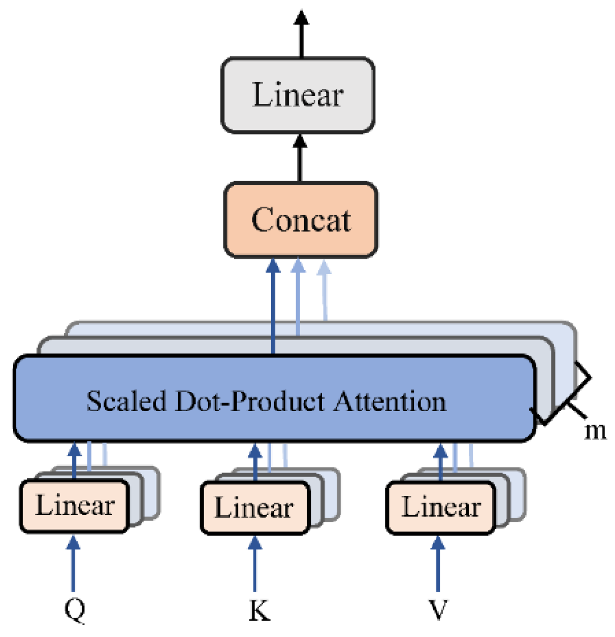
3.4.2. Multi-Head Attention

MHAT is the improvement of the traditional attention mechanism, and it has excellent performance. Figure 4 shows the architecture of the MHAT mechanism. Initially, by a linear transformation,$Q, K, \mathrm{and} V$ are the input of the scaled dot-product attention. Therefore, this operation computes one head at a time. Thus, it should be carried out $h$, which is called multi-head. The parameters $W$for each linear transformation of $Q, K, \mathrm{and} V$are different. Each scaled dot-product attention output of $m$time is concatenated, and the value obtained through a linear transformation is utilized as the output of the MHAT [47]. The formula can be expressed as shown below:

$${\mathrm{head}}_i=\mathrm{attention}\left(Q{W}_i^Q, K{W}_i^K, V{W}_i^Q\right)$$

(14)

$$\mathrm{Multihead}\left(Q,K,V\right)=\mathrm{concat}\left({\mathrm{head}}_i, \dots , {\mathrm{head}}_m\right)W^o$$

(15)

3.4.3. Self-Attention

In this approach, we employed a self-attention for extracting the inner relations of sentences in $\left(K=V=Q \right)$ [48]. For instance, every word that has been entered should carry out the attention computation with each other word of the sentence. Thus, the MHAT mechanism produces a weight matrix α and a feature representation$v$.

$$u_t=\tanh \left(W_s{H}_t+b_s\right)$$

(16)

$$v=\mathrm{Multihead}\left(U,U,U\right)$$

(17)

3.5. Global Average Pooling Layer

The fully connected network is the main architecture of the classification network, which contains an activation function, Softmax, for performing classification. The fully connected network function represents multiplying the vector, stretching the feature map into a vector, and eventually reducing its dimension. To obtain the corresponding result of every category, this vector is entered into a Softmax layer. The fully connected network has two major drawbacks: (i) the number of parameters is very large and thus reduces the training speed; (ii) it is easy to carry out overfitting. Based on the two problems mentioned above, the global average pooling can avoid the shortcomings to achieve the same effect and thus adds the sequences of input features to the averaging [49]. After presenting the MHAT mechanism to the sentence, the feature matrix of the corresponding output is $v$, and the feature vector of every word in the sentence is $v_1, v_2, \dots , v_n$. The global average pooling of the input sentence is shown below:

$$v_{\mathrm{gap}}=\mathrm{Global}\left(v1, v2, \dots ,v_n\right)$$

(18)

3.6. Softmax Layer

To predict sentiment analysis, we fed the output of vector $v_{\mathrm{gap}}$immediately into the Softmax layer, as shown in the equation below:

$$\widehat{y}=\mathrm{softmax}\left(W{V}_{\mathrm{gap}}+b\right)$$

(19)

To evaluate the proposed model, the purpose of cross-entropy was presented to reflect the gap among the predicted sentimental categories $\widehat{y}$ and the real sentimental categories $y$.

$$\mathrm{Loss}=-{\displaystyle \sum }_i{y}_i\log \widehat{y_i}$$

(20)

where $i$ represents the index number of the sentence.

The Bi-LSTM layer can determine the context to arrange the information of sequences. MHAT can learn information from the representation of sub-distances and various dimensions and fully capture long-space textual features, which can play a critical role in effectively improving the sentimental analysis capability of the model straightway. The pseudo-code of DNN–MHAT is shown in Algorithm 1.

Algorithm 1 Pseudo-code of DNN–MHAT

1: Build word embedding table using pre-trained word vectors with Equation (1);

2: Use the convolutional layer to obtain the feature sequences, using Equation (3);

3: Use BiLSTM to obtain the preceding contextual features $\overrightarrow{h_t}$ and the succeeding contextual features $\overleftarrow{h_t}$ from the feature sequences, using Equations (10)–(12);

4: Use multi-head attention layers to obtain the future context representation from the preceding and succeeding contextual features, using Equations (16) and (17);

5: Feed the output of multi-head attention into global average pooling, using Equation (18);

6: Feed the comprehensive context representations outputted from global average pooling into the Softmax function to obtain the class labels, using Equation (19);

7: Update parameters of the model using the loss function Equation (20) with the Adam method.

4. Experiments and Results

In this section, experiments conducted to assess the performance of the DNN–MHAT model for SA and text classification on different benchmarking datasets are described. The baseline methods and experimental setup, followed by a discussion of the results, are included in the following.

4.1. Experimental Setup

4.1.1. Datasets

Our study conducted sentiment analysis and text classification tasks utilizing long and short datasets. The details of the datasets are as follows:

APP: This dataset for Android applications [44] comprises 752,937 metadata and product reviews from Amazon.

Kindle: This dataset for Kindle Store [44] comprises 982,619 metadata and product reviews from Amazon.

Electronics: This dataset for Electronics [44] comprises 1,689,188 metadata and product reviews from Amazon.

CDs: This dataset for CDs and Vinyl [44] comprises 1,097,592 product metadata and product reviews from Amazon.

Airline Twitter: Airline Twitter sentiment dataset [44]. This dataset comprises 14,641 tweets about major U.S. airline problems from February 2015.

Sentiment140: This dataset was generated at Stanford University [44] by computer science graduate students, comprising 1,600,000 tweets classified into positive and negative categories.

Table 1. Details of the datasets utilized in our work.

Type	Dataset	Total	Positive	Negative
Review	APP	752,937	123,098	123,098
	Kindle	982,619	57,148	57,148
	Electronic	1,689,188	190,864	190,864
	CDs	1,097,592	92,766	92,766
Tweet	Airline Twitter	14,641	2363	2363
	Sentiment140	1,600,000	800,000	800,000

demonstrates the statistics of the datasets used in the proposed model and describes more details.

4.1.2. Data Pre-Processing

Data preprocessing considers an essential step in machine learning and data mining [50,51,52,53,54]. The reviews contain incomplete sentences; a large amount of noise; and weak wording, such as words without application, high repetition, imperfect words and incorrect grammar. Unstructured data also have an impact on sentiment classification results. Pre-processing the reviews is needed to maintain a regular structure and reduce such problems. Cleaning data with filters, splitting the data into parts for training and testing, and building data sets with favorite words are a few of the steps employed in our research. Without going into too much depth, we used the following techniques to prepare the data.

Tokenization

We divided the text into phrases, words, symbols, or other meaningful elements, thus forming a list of individual words per comment. In each comment, we then used each word as a feature for our training classifier.

Removing Stop Words

Comment contains some stop words that have no meaning, such as prepositions, and words that add no emotion value (or, also, able, etc.). The Natural Language Toolkit (NLTK) library provides a stop words dictionary, including words with neutral meaning neutral that are not suitable for sentiment analysis. To remove the stop words from the comment’s text, we checked each word in the list against the dictionary and excluded them.

Capitalization

Documents and texts containing many sentences and diverse capitalization can be a big problem when classifying big documents. The best approach to deal with inconsistent capitalization is to decapitalize each letter. This technique shows all words in the same feature distance to the text and document, but it poses a significant issue in the interpretation of some words (e.g., “US” (United States of America) to “us” (pronoun)).

4.1.3. Parameter Settings

The DNN–MHAT model was applied using the Tensorflow1.13.1 with Keras2.24 libraries written in Python 3.7.1 Language and an Ubuntu16.04 system with a CPU of Core Tetranuclear i7-7700k and a GPU of GTX1080 Ti GAMING X 11GB. To construct the input comment matrix $C$, the Tokenizer method uses 100,000 words. We assumed the 45 and 100 first words of comments in the tweet and review datasets by setting the padding sizes to 45 and 100, respectively. In the current study, the pre-trained and publicly available GloVe was utilized as the weights in the embedding layer. The “Gigaword 5 + Wikipedia 2014” version of GloVe was utilized, comprising six billion tokens and a vocabulary size of 400,000. For the embedding layer, the embedding size of 300 was used. Other parameter settings used in the proposed model are shown in

Table 2. Parameter settings.

Parameters	Value
Dimension $\left(d\right)$	100
Hidden unites Bi-LSTM	128
Word of comments for reviews	100
Word of comments for tweets	45
Convolutional layer	64
Window_size	7
Head $\left(m\right)$	8
Dropout $\left(\rho \right)$	0.5
Regularization coefficient $(ᵑ)$	0.001
Batch_size	64
Activation function	Relu
Patience	10
Kernel-size	4
Pool	2
Optimizer	Adam
Loss function	Binary cross-entropy

.

4.1.4. Evaluation Metrics

Four evaluation standards, Accuracy (Acc), Recall (Re), Precision (Pr), and F1 measure (F1), were employed for evaluating the performance of the proposed model. These standards are widely utilized in SA and text classification tasks. These standards are computed as follows [18]:

$$\mathrm{Pr}= \mathrm{TP}/\mathrm{TP}+\mathrm{FP},$$

(21)

$$\mathrm{Re}=\mathrm{TP}/\mathrm{TP}+\mathrm{FN},$$

(22)

$$\mathrm{F}1=2\mathrm{PrRe}/\mathrm{Pr}+\mathrm{Re},$$

(23)

$$\mathrm{Acc}=\mathrm{TP}+\mathrm{TN}/\mathrm{TP}+\mathrm{TN}+\mathrm{FP}+\mathrm{FN},$$

(24)

TN, FP, TP, and FN are true negative, false positive, true positive, and false negative, respectively [18].

4.2. Baseline Methods

In this work, we compared the DNN–MHAT model with five state-of-the-art DNN models that have been developed to detect the polarity of sentiment classification as listed below:

• IWV [15]: This model has been proposed for sentiment analysis, which comprises three convolution layers, a max-pooling layer, and a fully connected layer.
• SS-BED [13]: This model uses two equal LSTM layers on two various word embedding matrices for learning emotions and representations of semantic features. Then, LSTM output layers are fed as the input of a fully connected layer with one hidden layer for predicting sentiment categories.
• ARC [45]: This model applies a bidirectional GRU layer to the word vectors, and the outputs are fed into the attention layer. The attention Layer outputs are fed into a CNN layer followed by a max-pooling process and a fully connected layer.
• AC-BiLSTM [41]: This model uses a one-dimension CNN layer on the word embedding layer to extract local features, BiLSTM to extract long dependencies and an attention mechanism to focus on significant text domains.
• ABCDM [44]: This model first uses GloVe embedding as the weights to the embedding layer, then two bidirectional GRU and LSTM layers for extracting past and future contexts and an attention mechanism to focus on various words. Finally, convolution and pooling mechanisms are applied to extract local features’ static positions and reduce feature dimensions.

4.3. Results

In this section, the proposed model is compared with five baseline methods mentioned above for sentiment analysis with two types of datasets, four long reviews and two short tweets.

4.3.1. Long Review Analysis Results

Table 3. Results obtained for the Kindle dataset.

Methods	Class	Recall	Precision	F1	Accuracy
SS-BED	Pos	0.8308	0.9461	0.8827	0.8910
	Neg	0.9514	0.8521	0.8979
ARC	Pos	0.8718	0.9422	0.9254	0.9091
	Neg	0.9463	0.8811	0.9124
IWV	Pos	0.8779	0.9354	0.9046	0.9080
	Neg	0.9380	0.8870	0.9106
AC-Bi-LSTM	Pos	0.8553	0.9555	0.9018	0.9074
	Neg	0.9595	0.8705	0.9122
ABCDM	Pos	0.9088	0.9570	0.9322	0.9340
	Neg	0.9591	0.9134	0.9356
DNN–MHAT	Pos	0.9123	0.9612	0.9377	0.9372
	Neg	0.9614	0.9193	0.9394

,

Table 4. Results obtained for the APP dataset.

Methods	Class	Recall	Precision	F1	Accuracy
SS-BED	Pos	0.8937	0.9273	0.8994	0.9024
	Neg	0.9310	0.8814	0.9052
ARC	Pos	0.8618	0.9372	0.8977	0.9019
	Neg	0.9420	0.8724	0.9057
IWV	Pos	0.8720	0.9254	0.8977	0.9007
	Neg	0.9294	0.8793	0.9053
AC-Bi-LSTM	Pos	0.8558	0.9463	0.8983	0.9033
	Neg	0.9509	0.8692	0.9079
ABCDM	Pos	0.8945	0.9461	0.9196	0.9218
	Neg	0.9491	0.9000	0.9239
DNN–MHAT	Pos	0.9006	0.9505	0.9244	0.9256
	Neg	0.9523	0.9063	0.9304

,

Table 5. Results obtained for the CD dataset.

Methods	Class	Recall	Precision	F1	Accuracy
SS-BED	Pos	0.6997	0.8937	0.8747	0.8082
	Neg	0.9165	0.7535	0.8269
ARC	Pos	0.7699	0.8994	0.8288	0.8507
	Neg	0.9133	0.7999	0.8524
IWV	Pos	0.8021	0.8756	0.8362	0.8434
	Neg	0.8846	0.8189	0.8497
AC-Bi-LSTM	Pos	0.7524	0.9171	0.8254	0.8419
	Neg	0.9314	0.7917	0.8553
ABCDM	Pos	0.8522	0.9162	0.8829	0.8870
	Neg	0.9218	0.8622	0.8909
DNN–MHAT	Pos	0.8578	0.9188	0.8906	0.8913
	Neg	0.9306	0.8692	0.8959

and

Table 6. Results obtained for the Electronic dataset.

Methods	Class	Recall	Precision	F1	Accuracy
SS-BED	Pos	0.8351	0.8964	0.8633	0.8684
	Neg	0.9017	0.8476	0.8728
ARC	Pos	0.8184	0.9115	0.8615	0.8689
	Neg	0.9194	0.8365	0.8754
IWV	Pos	0.8292	0.9092	0.8664	0.8725
	Neg	0.9159	0.8443	0.8779
AC-Bi-LSTM	Pos	0.8280	0.9253	0.8736	0.8804
	Neg	0.9327	0.8449	0.8864
ABCDM	Pos	0.8701	0.9387	0.9029	0.9065
	Neg	0.9428	0.8791	0.9097
DNN–MHAT	Pos	0.8777	0.9411	0.9092	0.9112
	Neg	0.9482	0.8821	0.9127

show the results obtained for four long review datasets.

In Table 3, Table 4, Table 5 and Table 6, DNN–MHAT achieved good performance in terms of accuracy, as 0.32%, 0.47%, 0.43%, and 0.38% on Kindle, Electronics, CD, and App datasets, respectively. For the F1 scale, the improvements are 0.55%, 0.63%, 0.77%, and 0.48% for the positive class and 0.38%, 0.30%, 0.50%, and 0.65% for the negative class on Kindle, Electronics, CD, and App datasets, respectively. As indicated above for accuracy and F1 scale, our DNN–MHAT outperformed the other five methods. It can be seen that these improvements were mainly derived from (i) handling long dependencies in text utilizing bidirectional LSTM layers, (ii) employing local features of varying lengths by applying CNN layers of different sizes, and (iii) assigning weights to words in the review according to their significance achieved from the multi-head attention (MHAT) mechanism layer.

4.3.2. Short Tweet Analysis Results

Table 7. Results obtained for the Airline Twitter dataset.

Methods	Class	Recall	Precision	F1	Accuracy
SS-BED	Pos	0.9470	0.9403	0.9436	0.9100
	Neg	0.7658	0.7913	0.7772
ARC	Pos	0.9578	0.9460	0.9518	0.9229
	Neg	0.7870	0.8309	0.8070
IWV	Pos	0.9369	0.9367	0.9355	0.8985
	Neg	0.7489	0.7861	0.7542
AC-Bi-LSTM	Pos	0.9503	0.9459	0.9480	0.9172
	Neg	0.7888	0.8061	0.7693
ABCDM	Pos	0.9574	0.9520	0.9545	0.9275
	Neg	0.8112	0.8369	0.8209
DNN–MHAT	Pos	0.9608	0.9588	0.9603	0.9302
	Neg	0.8167	0.8411	0.8261

and

Table 8. Results obtained for the Sentiment140 dataset.

Methods	Class	Recall	Precision	F1	Accuracy
SS-BED	Pos	0.8883	0.7601	0.8191	0.8083
	Neg	0.7192	0.8657	0.7855
ARC	Pos	0.9085	0.7314	0.8103	0.7873
	Neg	0.6660	0.8795	0.7577
IWV	Pos	0.8954	0.7588	0.8213	0.8052
	Neg	0.7149	0.8727	0.7857
AC-Bi-LSTM	Pos	0.8871	0.7766	0.8280	0.8157
	Neg	0.7443	0.8686	0.8014
ABCDM	Pos	0.9019	0.7729	0.8323	0.8182
	Neg	0.7444	0.8825	0.8076
DNN–MHAT	Pos	0.9085	0.7782	0.8392	0.8217
	Neg	0.7478	0.8896	0.8112

show the results obtained for two short tweet datasets.

As shown in Table 7 and Table 8, DNN–MHAT achieved good performance in terms of accuracy, 0.35% and 0.27% on Sentiment140 and Airline Twitter datasets, respectively. For the F1 scale, the improvements are 0.69% and 0.58% for the positive class and 0.36% and 0.52% for the negative class on Sentiment140 and Airline Twitter datasets, respectively. As indicated above for accuracy and F1 scale, our DNN–MHAT outperformed the other five methods. As shown in the results in Table 7 and Table 8 for accuracy and F1 scales, DNN–MHAT outperformed the other five models in short tweets of Twitter datasets.

4.3.3. Ablation Study

To test the effectiveness of our model, we report the verification loss value, accuracy rate, training loss value, and training accuracy rate for two datasets, including the CD dataset and the Airline tweet dataset, as shown in Figure 5, Figure 6, Figure 7 and Figure 8.

We also evaluated our DNN–MHAT model using a dataset from a different language. We ran the DNN–MHAT model on the ASTD [55] dataset in the Arabic language. For a fair comparison, we embedded sentences using AraBERT.

Table 9. The accuracy of AraBERT DNN–MHAT for ASTD Arabic dataset.

Model	Accuracy%
Arabic-BERT Base [56]	71.4
AraBERT [57]	92.6
Arabic BERT [58]	91
Our model	92.8

shows the performance of our model, which achieved a better result.

To illustrate the performance of our proposed DNN–MHAT model, we executed our model using different embedding layer sizes, namely, 50,100, 200, and 300, as shown in Figure 9 and Figure 10.

The various embedding sizes have a certain effect on the proposed model’s performance, so the DNN–MHAT model’s accuracy was evaluated on two datasets when the number of epochs is equal to 5, 6, 7, 8, 9, and 10. As we can see in Figure 9 and Figure 10, the embedding size of 300 performs better than the other embedding sizes in both CD and Airline datasets.

The experiments illustrate that the GloVe pre-trained embedding, especially when the embedding size is set to 300, can achieve better results than other embedding sizes.

4.3.4. Discussion

The results show that the DNN–MHAT model outperformed the other five models in terms of both F1 measures and accuracy with Twitter datasets. However, the improvements are less compared to utilizing the review datasets. The main reason for this is that the Twitter datasets contain a small number of words. As mentioned above, the DNN–MHAT model does not provide important improvements when utilizing short comments. The first feature extraction layer in this model is an RNN-based network, which is evolved to capture long dependencies.

Due to the ability of BiLSTM to access both the previous and the following context, the information obtained by BiLSTM can be considered two different representations of the text. Moreover, employing a multi-head attention mechanism for each text representation can better focus on the significant related information and avoid the reciprocal intervention in the various representations. Thus, the multi-head attention mechanism in our model makes the determination of text semantics more accurate. Hence, our model effectually improves the accuracy of text classification and sentiment analysis.

However, our study was limited to document-level sentiment analysis. In this study, we did not consider the aspect-level sentiment. We leave this part for future work.

5. Conclusions and Future Work

For sentiment analysis, we propose a hybrid model that combines a deep neural network with a multi-head attention (DNN–MHAT) mechanism to tackle text data sparsity and high dimensionality problems. First, DNN–MHAT exploits pre-trained GloVe word embedding vectors as the primary weights into the embedding layer. Second, the CNN layer was used for extracting the local features of position invariants. Third, a recurrent Bi-LSTM unit was used for capturing the actual context of the text. After that, a multi-head attention mechanism was applied to the outputs of Bi-LSTM to capture the words in a text that are significantly related to long space and encode dependencies. The purpose of this is to add effect weights to the generated text concatenation. The MHAT provides an emphasis on variant words in a comment and hence makes the semantic representations more informative. Finally, a global average pooling with a sigmoid classifier is applied to transform the vector into a high-level sentiment representation while avoiding model overfitting and implementing the sentiment polarity classification of comments.

This study focused on detecting the polarity of sentiment analysis at the document level. In future work, we propose the verification of the effectiveness of our DNN–MHAT model for other levels, such as sentence-level and aspect-level sentiment analysis, and other sentiment analysis tasks, such as helpfulness and rating prediction.

References

1. Hussain, A.; Cambria, E. Semi-supervised learning for big social data analysis. Neurocomputing 2018, 275, 1662–1673. [Google Scholar] [CrossRef] [Green Version]
2. Xia, Y.; Cambria, E.; Hussain, A.; Zhao, H. Word polarity disambiguation using Bayesian model and opinion-level features. Cogn. Comput. 2015, 7, 369–380. [Google Scholar] [CrossRef]
3. Chaturvedi, I.; Ragusa, E.; Gastaldo, P.; Zunino, R.; Cambria, E. Bayesian network based extreme learning machine for subjectivity detection. J. Frankl. Inst. 2018, 355, 1780–1797. [Google Scholar] [CrossRef]
4. Song, M.; Park, H.; Shin, K.-S. Attention-based long short-term memory network using sentiment lexicon embedding for aspect-level sentiment analysis in Korean. Inf. Process. Manag. 2019, 56, 637–653. [Google Scholar] [CrossRef]
5. Pennington, J.; Socher, R.; Manning, C.D. GloVe: Global vectors for word representation. In Proceedings of the 2014 Conference on Empirical Methods in Natural Language Processing (EMNLP), Doha, Qatar, 25–29 October 2014; pp. 1532–1543. [Google Scholar] [CrossRef]
6. Khatua, A.; Khatua, A.; Cambria, E. A tale of two epidemics: Contextual Word2Vec for classifying twitter streams during outbreaks. Inf. Process. Manag. 2019, 56, 247–257. [Google Scholar] [CrossRef]
7. Xing, F.; Cambria, E.; Welsch, R.E. Intelligent asset allocation via market sentiment views. IEEE Comput. Intell. Mag. 2018, 13, 25–34. [Google Scholar] [CrossRef]
8. Voulodimos, A.; Doulamis, N.; Doulamis, A.; Protopapadakis, E. Deep learning for computer vision: A brief review. Comput. Intell. Neurosci. 2018, 2018, 7068349. [Google Scholar] [CrossRef]
9. Chaturvedi, I.; Satapathy, R.; Cavallari, S.; Cambria, E. Fuzzy commonsense reasoning for multimodal sentiment analysis. Pattern Recognit. Lett. 2019, 125, 264–270. [Google Scholar] [CrossRef]
10. Yadav, A.; Vishwakarma, D.K. Sentiment analysis using deep learning architectures: A review. Artif. Intell. Rev. 2020, 53, 4335–4385. [Google Scholar] [CrossRef]
11. Hochreiter, S.; Schmidhuber, J. Long short-term memory. Neural Comput. 1997, 9, 1735–1780. [Google Scholar] [CrossRef]
12. Cambria, E.; Wang, H.; White, B. Guest editorial: Big social data analysis. Knowl.-Based Syst. 2014, 69, 1–2. [Google Scholar] [CrossRef]
13. Chatterjee, A.; Gupta, U.; Chinnakotla, M.K.; Srikanth, R.; Galley, M.; Agrawal, P. Understanding emotions in text using deep learning and big data. Comput. Hum. Behav. 2019, 93, 309–317. [Google Scholar] [CrossRef]
14. Hameed, Z.; Garcia-Zapirain, B. Sentiment classification using a single-layered BiLSTM model. IEEE Access 2020, 8, 73992–74001. [Google Scholar] [CrossRef]
15. Rezaeinia, S.M.; Rahmani, R.; Ghodsi, A.; Veisi, H. Sentiment analysis based on improved pre-trained word embeddings. Expert Syst. Appl. 2019, 117, 139–147. [Google Scholar] [CrossRef]
16. Vaswani, A.; Shazeer, N.; Parmar, N.; Uszkoreit, J.; Jones, L.; N. Gomez, A.; Kaiser, Ł.; Polosukhin, I. Attention is all you need. In Advances in Neural Information Processing Systems, Proceedings of the Annual Conference on Neural Information Processing Systems, Long Beach, CA, USA, 4–9 December 2017; pp. 5998–6008. Available online: https://proceedings.neurips.cc/paper/2017/hash/3f5ee243547dee91fbd053c1c4a845aa-Abstract.html (accessed on 14 October 2021).
17. Chauhan, U.A.; Afzal, M.T.; Shahid, A.; Abdar, M.; Ehsan Basiri, M.; Zhou, X. A comprehensive analysis of adverb types for mining user sentiments on amazon product reviews. World Wide Web 2020, 23, 1811–1829. [Google Scholar] [CrossRef]
18. Liu, B. Sentiment Analysis: Mining Opinions, Sentiments, and Emotions; Cambridge University Press: Cambridge, UK, 2020. [Google Scholar]
19. Zhao, W.; Peng, H.; Eger, S.; Cambria, E.; Yang, M. Towards scalable and reliable capsule networks for challenging NLP applications. arXiv 2019, 1906, 02829. [Google Scholar]
20. Georgieva-Trifonova, T.; Duraku, M. Research on N-grams feature selection methods for text classification. IOP Conf. Ser. Mater. Sci. Eng. 2021, 1031, 012048. [Google Scholar] [CrossRef]
21. Mishra, S.; Mallick, P.; Tripathy, H.; Bhoi, A.; González-Briones, A. Performance evaluation of a proposed machine learning model for chronic disease datasets using an integrated attribute evaluator and an improved decision tree classifier. Appl. Sci. 2020, 10, 8137. [Google Scholar] [CrossRef]
22. Poria, S.; Chaturvedi, I.; Cambria, E.; Bisio, F. Sentic LDA: Improving on LDA with semantic similarity for aspect-based sentiment analysis. In Proceedings of the 2016 International Joint Conference on Neural Networks (IJCNN 2016), Vancouver, BC, Canada, 24–29 July 2016; IEEE: Manhattan, NY, USA, 2016; pp. 4465–4473. [Google Scholar] [CrossRef]
23. Chaturvedi, I.; Ong, Y.-S.; Tsang, I.W.; Welsch, R.E.; Cambria, E. Learning word dependencies in text by means of a deep recurrent belief net-work. Knowl. Based Syst. 2016, 108, 144–154. [Google Scholar] [CrossRef]
24. Basiri, M.E.; Arman, K. Words are important: Improving sentiment analysis in the Persian language by lexicon refining. ACM Trans. Asian Low Resour. Lang. Inf. Process. 2018, 17, 1–18. [Google Scholar] [CrossRef]
25. Rajabi, Z.; Valavi, M.R. A survey on sentiment analysis in Persian: A comprehensive system perspective covering challenges and advances in resources and methods. Cogn. Comput. 2021, 13, 882–902. [Google Scholar] [CrossRef]
26. Basiri, M.E.; Kabiri, A. HOMPer: A new hybrid system for opinion mining in the Persian language. J. Inf. Sci. 2020, 46, 101–117. [Google Scholar] [CrossRef]
27. Abdar, M.; Basiri, M.E.; Yin, J.; Habibnezhad, M.; Chi, G.; Nemati, S.; Asadi, S. Energy choices in Alaska: Mining people’s perception and attitudes from geotagged tweets. Renew. Sustain. Energy Rev. 2020, 124, 109781. [Google Scholar] [CrossRef]
28. Cambria, E.; Li, Y.; Xing, F.Z.; Poria, S.; Kwok, K. SenticNet 6: Ensemble application of symbolic and subsymbolic AI for sentiment analysis. In Proceedings of the 29th ACM International Conference on Information and Knowledge Management, Online, 19–23 October 2020; pp. 105–114. [Google Scholar] [CrossRef]
29. Zhang, L.J.; Ghosh, R.; Dekhil, M.; Hsu, M.; Liu, B. Combining lexicon-based and learning-based methods for Twitter sentiment analysis. In Technical Report HPL-2011; HP Laboratories: Palo Alto, CA, USA, 2011; p. 89. [Google Scholar]
30. Mudinas, A.; Zhang, D.; Levene, M. Combining lexicon and learning based approaches for concept-level sentiment analysis. In Proceedings of the First International Workshop on Issues of Sentiment Discovery and Opinion Mining, Beijing, China, 12 August 2012; pp. 1–8. [Google Scholar]
31. Jameel, M.; Bouraoui, Z.; Schockaert, S. Unsupervised learning of distributional relation vectors. In Proceedings of the 56th Annual Meeting of the Association for Computational Linguistics, Melbourne, Australia, 15–20 July 2018; Volume 1, pp. 23–33. [Google Scholar] [CrossRef] [Green Version]
32. Sharma, R.; Somani, A.; Kumar, L.; Bhattacharyya, P. Sentiment intensity ranking among adjectives using sentiment bearing word embeddings. In Proceedings of the 2017 Conference on Empirical Methods in Natural Language Processing, Copenhagen, Denmark, 7–11 September 2017; pp. 547–552. [Google Scholar] [CrossRef] [Green Version]
33. Tang, D.; Wei, F.; Qin, B.; Yang, N.; Liu, T.; Zhou, M. Sentiment Embeddings with Applications to Sentiment Analysis. IEEE Trans. Knowl. Data Eng. 2015, 28, 496–509. [Google Scholar] [CrossRef]
34. Xiong, S.; Lv, H.; Zhao, W.; Ji, D. Towards Twitter sentiment classification by multi-level sentiment-enriched word embeddings. Neurocomputing 2018, 275, 2459–2466. [Google Scholar] [CrossRef] [Green Version]
35. Dragoni, M.; Petrucci, G. A neural word embeddings approach for multi-domain sentiment analysis. IEEE Trans. Affect. Comput. 2017, 8, 457–470. [Google Scholar] [CrossRef]
36. Young, T.; Hazarika, D.; Poria, S.; Cambria, E.l. Recent trends in deep learning based natural language processing. IEEE Comput. Intell. Mag. 2018, 13, 55–75. [Google Scholar] [CrossRef]
37. Lu, C.; Huang, H.; Jian, P.; Wang, D.; Guo, D. A P-LSTM neural network for sentiment classification. In Pacific Asia Conference on Knowledge Discovery and Data Mining; Springer: Cham, Switzerland, 2017; pp. 524–533. [Google Scholar]
38. Xu, J.; Chen, D.; Qiu, X.; Huang, X. Cached Long Short-Term Memory Neural Networks for Document-Level Sentiment Classification. In Proceedings of the 2016 Conference on Empirical Methods in Natural Language Processing, Austin, TX, USA, 1–5 November 2016. [Google Scholar] [CrossRef] [Green Version]
39. Tang, D.; Wei, F.; Yang, N.; Zhou, M.; Liu, T.; Qin, B. Learning sentiment-specific word embedding for twitter sentiment classification. In Proceedings of the 52nd Annual Meeting of the Association for Computational Linguistics, Baltimore, MD, USA, 22–27 June 2014; pp. 1555–1565. [Google Scholar] [CrossRef]
40. Mikolov, T.; Sutskever, I.; Chen, K.; Corrado, G.S.; Dean, J. Distributed representations of words and phrases and their compositionality. In Proceedings of the Advances in Neural Information Processing Systems, Lake Tahoe, NV, USA, 5–8 December 2013; pp. 3111–3119. Available online: https://proceedings.neurips.cc/paper/2013/hash/9aa42b31882ec039965f3c4923ce901b-Abstract.html (accessed on 14 October 2021).
41. Liu, G.; Guo, J. Bidirectional LSTM with attention mechanism and convolutional layer for text classification. Neurocomputing 2019, 337, 325–338. [Google Scholar] [CrossRef]
42. Zhou, X.; Wan, X.; Xiao, J. Attention-based LSTM network for cross-lingual sentiment classification. In Proceedings of the 2016 Conference on Empirical Methods in Natural Language Processing, Austin, TX, USA, 1–4 November 2016; pp. 247–256. [Google Scholar] [CrossRef]
43. Yang, Z.; Yang, D.; Dyer, C.; He, X.; Smola, A.J.; Hovy, E.H. Hierarchical attention networks for document classification. In Proceedings of the 2016 Conference of the North American Chapter of the Association for Computational Linguistics: Human Language Technologies, San Diego, CA, USA, 12–17 June 2016; pp. 1480–1489. [Google Scholar] [CrossRef] [Green Version]
44. Basiri, M.E.; Nemati, S.; Abdar, M.; Cambria, E.; Acharrya, U.R. ABCDM: An Attention-based Bidirectional CNN-RNN Deep model for sentiment analysis. Future Gener. Comput. Syst. 2021, 115, 279–294. [Google Scholar] [CrossRef]
45. Wen, S.; Li, J. Recurrent convolutional neural network with attention for twitter and yelp sentiment classification: ARC model for sentiment classification. In Proceedings of the 2018 International Conference on Algorithms, Computing and Artificial Intelligence, Sanya, China, 21–23 December 2018; pp. 1–7. [Google Scholar] [CrossRef]
46. Graves, A.; Navdeep, J.; Abdel-Rahman, M. Hybrid speech recognition with deep bidirectional LSTM. In Proceedings of the Workshop on Automatic Speech Recognition and Understanding, Olomouc, Czech Republic, 8–12 December 2013; pp. 273–278. [Google Scholar] [CrossRef]
47. Wan, X. Co-training for cross-lingual sentiment classification. In Proceedings of the 47th Annual Meeting of the Association for Computational Linguistics and the 4th International Joint Conference on Natural Language Processing of the AFNLP, Suntec, Singapore, 2–7 August 2009; pp. 235–243. Available online: https://aclanthology.org/P09-1027/ (accessed on 14 October 2021).
48. Sutskever, I.; Vinyals, O.; Le, Q.V. Sequence to sequence learning with neural net-works. In Proceedings of the Advances in Neural Information Processing Systems, Montreal, QC, Canada, 8–13 December 2014; pp. 3104–3112. Available online: https://proceedings.neurips.cc/paper/2014/hash/a14ac55a4f27472c5d894ec1c3c743d2-Abstract.html (accessed on 14 October 2021).
49. Kinga, D.; Adam, J.B. A method for stochastic optimization. In Proceedings of the 3rd International Conference on Learning Representations, San Diego, CA, USA, 7–9 May 2015; Available online: https://arxiv.org/abs/1412.6980 (accessed on 14 October 2021).
50. Bahaghighat, M.; Mirfattahi, M.; Akbari, L.; Babaie, M. Designing quality control system based on vision inspection in pharmaceutical product lines. In Proceedings of the 2018 International Conference on Computing, Mathematics and Engineering Technologies (iCoMET), Sukkur, Pakistan, 3–4 March 2018; pp. 1–4. [Google Scholar] [CrossRef]
51. Babaie, M.; Shiri, M.E.; Bahaghighat, M. A new descriptor for UAV images mapping by applying discrete local radon. In Proceedings of the 2018 8th Conference of AI & Robotics and 10th RoboCup Iranopen International Symposium (IRANOPEN), Qazvin, Iran, 10 April 2018. [Google Scholar] [CrossRef]
52. Gupta, G.; Sumit, M. Text document tokenization for word frequency count using rapid miner (taking resume as an example). Int. J. Comput. Appl. 2015, 975, 8887. [Google Scholar]
53. Tanu, V.; Renu, R.; Gaur, D. Tokenization and filtering process in RapidMiner. Int. J. Appl. Inf. Syst. 2014, 7, 16–18. Available online: https://research.ijais.org/volume7/number2/ijais14-451139.pdf (accessed on 14 October 2021).
54. Ma, T.; Al-Sabri, R.; Zhang, L.; Marah, B.; Al-Nabhan, N. The impact of weighting schemes and stemming process on topic modeling of Arabic long and short texts. ACM Trans. Asian Low Resource Lang. Inf. Process. 2020, 19, 1–23. [Google Scholar] [CrossRef]
55. Nabil, M.; Mohamed, A.; Amir, A. Astd: Arabic sentiment tweets dataset. In Proceedings of the 2015 Conference on Empirical Methods in Natural Language Processing, Lisbon, Portugal, 17–21 September 2015; pp. 2515–2519. [Google Scholar] [CrossRef]
56. Safaya, A.; Abdullatif, M.; Yuret, D. KUISAIL at SemEval-2020 Task 12: BERT-CNN for offensive speech identification in social media. arXiv 2020, 2020, 2054–2059. [Google Scholar] [CrossRef]
57. Antoun, W.; Baly, F.; Hajj, H. AraBERT: Transformer-based model for Arabic language understanding. arXiv 2020, 2020, 00104. [Google Scholar]
58. Chouikhi, H.; Hamza, C.; Fethi, J. Arabic sentiment analysis using BERT model. In Proceedings of the International Conference on Computational Collective Intelligence, Kallithea, Greece, 29 September–1 October 2021; Springer: Cham, Switzerland, 2021; pp. 621–632. [Google Scholar] [CrossRef]
Figure 1. The structure of the DNN–MHAT model.
Asi 04 00085 g001
Figure 2. The flowchart of our proposed model (DNN–MHAT).
Asi 04 00085 g002
Figure 3. Illustration of an LSTM model (a) and a Bi-LSTM model (b).
Asi 04 00085 g003
Figure 4. The architecture of the MHAT mechanism.
Asi 04 00085 g004
Figure 5. The training loss of the CD dataset.
Asi 04 00085 g005
Figure 6. The training accuracy of the CD dataset.
Asi 04 00085 g006
Figure 7. The training loss of the Airline tweet.
Asi 04 00085 g007
Figure 8. The training accuracy of the Airline tweet dataset.
Asi 04 00085 g008
Figure 9. The accuracy of the CD dataset on various embedding sizes with different epochs.
Asi 04 00085 g009
Figure 10. The accuracy of the Airline tweet dataset on various embedding sizes with different epochs.
Asi 04 00085 g010