Performance of Different SLAM Algorithms for Indoor and Outdoor Mapping Applications

Abstract

Indoor and outdoor mapping studies can be completed relatively quickly, depending on the developments in Mobile Mapping Systems. Especially in indoor environments where high accuracy GNSS positions cannot be used, mapping studies can be carried out with SLAM algorithms. Although there are many different SLAM algorithms in the literature, each can produce results with different accuracy according to the mapped environment. In this study, 3D maps were produced with LOAM, A-LOAM, and HDL Graph SLAM algorithms in different environments such as long corridors, staircases, and outdoor environments, and the accuracies of the maps produced with different algorithms were compared. For this purpose, a mobile mapping platform using Velodyne VLP-16 LIDAR sensor was developed, and the odometer drift, which causes loss of accuracy in the data collected, was minimized by loop closure and plane detection methods. As a result of the tests, it was determined that the results of the LOAM algorithm were not as accurate as those of the A-LOAM and HDL Graph SLAM algorithms. Both indoor and outdoor environments and the A-LOAM results’ accuracy were two times better than HDL Graph SLAM results.

1. Introduction

With the development of mobile mapping technology, fast and high accuracy mapping and precise 3D modelling have become possible. Mobile mapping systems have become popular in many areas, such as cartography, autonomous vehicles, and virtual and augmented reality environments.

The main challenge for mapping the environment with a mobile mapping system is calculating the position and orientation of the LIDAR. Simultaneous Localization and Mapping (SLAM) based approaches are sometimes used in the literature for this purpose. In some approaches, only point cloud data from LIDAR is sufficient to solve this problem, while in others, additional sensor data is needed. Algorithms using only LIDAR data are based on matching the point cloud common features in the t-time with the point cloud features extracted from the t − 1 time. Algorithms that solve this problem using LIDAR and IMU receive the rotation and acceleration data of LIDAR from the IMU and create a point cloud.

Currently, different SLAM algorithms such as LOAM, A-LOAM, ICP, BLAM, and HDL Graph SLAM are used for 3D localization and mapping [1,2,3,4]. Mossmann F. and Stiller C. [5] used Velodyne HDL-64E LIDAR combined with the ICP algorithm for producing precise maps. Hong et al. [6] proposed a novel method, namely VICP, which enhances the ICP algorithm by updating the velocity for avoiding an accumulated tracking error during motion. They have stated that VICP provides more accurate tracking, especially for faster motion than the original ICP algorithms. Segal et al. [7] combined the ICP algorithm with the local planar structure of the scans and named the new method Generalized-ICP. They have shown that in a range of both simulated and real-world experiments, Generalized-ICP increased the map accuracy. Minguez et al. [8] offered a metric-based matching algorithm to estimate the robot planar displacement by matching dense two-dimensional range scans. They have improved the classical ICP method in robustness, precision, convergence rate, and computation time. Nüchter et al. [9] used six degrees of freedom, namely x, y, and z coordinates and the roll, pitch, and yaw angles for localization and mapping of robots. They have combined ICP scan matching with a loop detection model. Yang et al. [10] developed a real-time LIDAR inertial odometry system (RTLIO) to generate high precision and high-frequency odometry system for the feedback control of UAVs in an indoor environment. They stated that RTLIO could outperform ALOAM and LOAM by exhibiting a shorter time delay and greater position accuracy. Montemerlo et al. [11] presented a FastSLAM algorithm that recursively estimates the full posterior distribution over robot pose and landmark locations yet scales logarithmically with the number of landmarks in the map. Wang et al. [12] designed a mobile LIDAR scanning system for extracting the canopy morphology and tree crown parameters. They have integrated LIDAR with IMU and GNSS sensors.

BLAM is based on the loop closure algorithm and uses ICP as the point cloud matching method [3]. For the loop closure algorithm to work in BLAM, the starting and ending points must be within the specified tolerance limits.

The LOAM algorithm presented in [1] used both low drift and low computational complexity without high accuracy ranging or inertial measurements. The main principle of LOAM is dividing the simultaneous localization and mapping problem into two algorithms. One algorithm performs odometry to estimate the velocity, while another performs fine matching and registration of point cloud in real-time. The authors have stated that motion estimation drift can be fixed by integrating the loop closure methods.

A-LOAM is an Advanced implementation of LOAM, which uses the Eigen and Ceres Solver framework to simplify code structure [2].

The Graph-based SLAM approach reduces raw sensor data to a simplified prediction problem [13]. The HDL Graph SLAM is an advanced implementation of 3D Graph SLAM with NDT scan matching-based odometry estimation and loop detection [14]. With the loop closure algorithm, HDL Graph SLAM provides the distribution of accumulated errors depending on the distance. It also supports GPS and IMU sensor data and can perform floor plane detection in indoor mapping applications.

With the Interactive SLAM algorithm developed by Koide et al. [15], it is possible to correct the drifts manually or automatically in the 3D maps. Corrections can be made using loop closure algorithms in the data collected with any SLAM-based mobile mapping system. In addition, plane-based map correction techniques can increase position accuracy by reducing noise in the maps.

In this study, the performances of LOAM, A-LOAM, and HDL Graph SLAM algorithms in mapping studies applied in indoor and outdoor environments were tested, and the effects of loop closure and plane detection methods on the accuracies of maps were examined. Similar studies have been carried out on this subject; for instance, Sobczak et al. [16] studied the accuracy of the Google Cartographer SLAM algorithm using the Velodyne VLP-16 sensor. Arshad and Kim [17] studied deep learning-based methods for loop closure detection for visual and LIDAR SLAM. These authors consequently stated that the learning-based methods are computationally expensive, and their performance is dependent on the dataset used for training the network.

2. Materials and Methods

In order to create a map with a moving LIDAR sensor, it is necessary to know the location of the LIDAR. However, a map is needed to know the LIDAR location, which creates a dilemma in robotics. SLAM solves this problem by simultaneously performing localization and creation of an unknown environment map [18]. With a mobile LIDAR sensor, both the mapping process and the accuracy of the map are contingent on the solution of the SLAM problem. In this study, open-source LOAM, A-LOAM, and HDL Graph SLAM algorithms were used to create indoor and outdoor environments maps.

2.1. HDL Graph SLAM

HDL Graph SLAM is an open-source ROS (Robot Operating System) package for real-time 6DOF SLAM using a 3D LIDAR [14]. It is based on 3D Graph SLAM with NDT [19] scan matching-based odometry estimation and loop detection.

In the HDL Graph SLAM algorithm, the point cloud is downsampled, and then the sensor pose is estimated by applying the scan matching between consecutive frames. Floor plans are detected by the RANSAC method simultaneously. Finally, estimated odometry and detected floor planes are used for creating map points [2].

2.2. LOAM SLAM

The LOAM algorithm is developed to create maps with low odometry drift. In this method, a dense point cloud is created with low odometry drift and low computational complexity without the need for additional sensor measurements [1]. To reduce the computational complexity and optimize the performance, the LOAM algorithm is divided into two main parts. The first part generates high-frequency but low-accuracy odometry data to determine the speed and position of the LIDAR. The second part accurately maps the point clouds using low frequency and high accuracy odometry data.

After registering point cloud data from LIDAR, the LIDAR odometry algorithm calculates the current speed, orientation, and position of the LIDAR. An additional correction is introduced to point clouds with calculated odometry data. The final point cloud is obtained by integrating two algorithms running at 10 Hz and 1 Hz. The most important factor affecting the spatial accuracy of the obtained point clouds is the accuracy of the odometry calculation. The odometry calculation used in the LOAM algorithm is examined under two main headings: feature extraction and feature matching [1].

2.3. Interactive SLAM

The interactive SLAM algorithm uses odometry and point cloud data to create ‘vertex’ at certain intervals and calculate the RMS value by creating an edge connection between the vertexes. The positions of the vertexes can be changed or corrected according to these edge connections. The point cloud matching algorithms such as ICP, GICP, NDT, NDT OMP are used to connect the edges of vertexes [17].

Two loop closure methods are used in the interactive SLAM algorithm. The first method is the manual loop closure. In this method, vertexes are selected manually, and their positions are corrected using point cloud matching algorithms. Unlike the manual loop closure method, the automatic loop closure method automatically creates edges between vertexes at specified distances. Threshold values and parameters selected in automatic loop closure algorithms are critical. If the threshold value is selected as high, each vertex will match each other at the specified distance limit, and errors will accumulate, causing unwanted drifts. If the value selected is too low, the paired vertexes will be very few, and no correction will be made [17].

With the plane detection method in the interactive SLAM algorithm, conditions such as perpendicularity and parallelism can be detected, and point clouds can be corrected. The map can be updated by determining the minimum elevation using the planes defined as the ground. Likewise, using the surfaces defined as ceilings, the maximum elevation can be determined, and the map can be updated by filtering the values greater than this elevation.

2.4. Mobile Mapping System

In the mobile mapping system designed in this study, the Velodyne VLP-16 LIDAR sensor, a laptop (Intel i3 processor and 4GB RAM), and a lipo battery mounted on a backpack were used. The LIDAR sensor is mounted on the bag with a 360-degree viewing angle to collect maximum point cloud data. A laptop in the bag was connected to the LIDAR sensor with an ethernet cable, and the LIDAR sensor was powered by a lipo battery. The prototype mobile mapping system used in this study is given in Figure 1.

3. Experiments

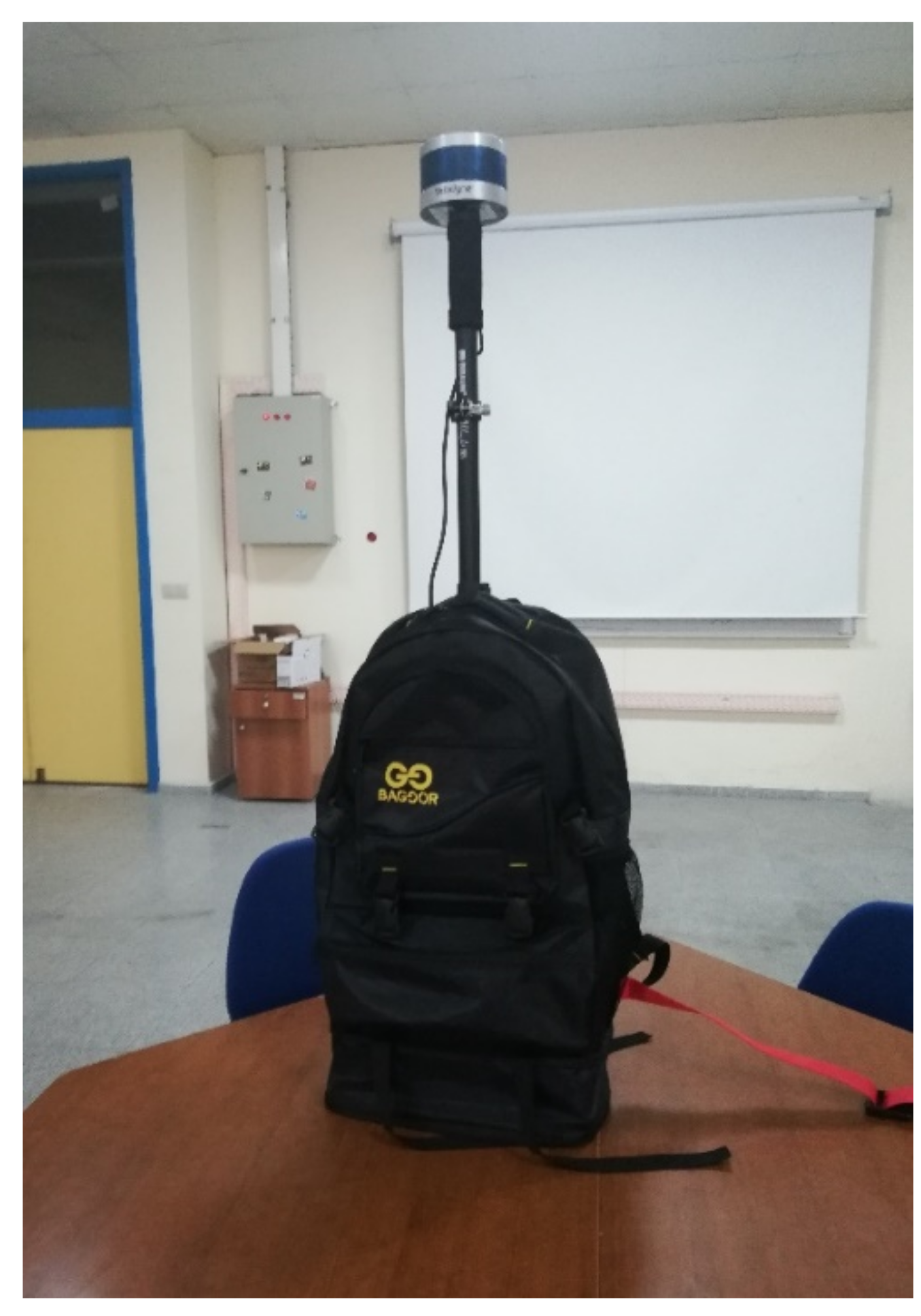
In this study, 3D maps were produced with LOAM, A-LOAM, and HDL Graph SLAM algorithms in different environments such as long corridors, staircases, and outdoor environments. The effects of loop closure and plane detection methods on the accuracies of maps were examined by applying the interactive SLAM algorithm to resulting point clouds. Measurements were made with the mobile mapping system given in Figure 1, and the obtained data were processed with LOAM, A-LOAM, and HDL Graph SLAM algorithms. To determine the effects of loop closure and plane detection methods, an interactive SLAM algorithm was applied to the point clouds, and the results were examined. For determining the accuracy of different SLAM algorithms in different environments, distance controls were made on the 3D maps, and the accuracy of the methods was determined.

3.1. Experiments in Long Corridor

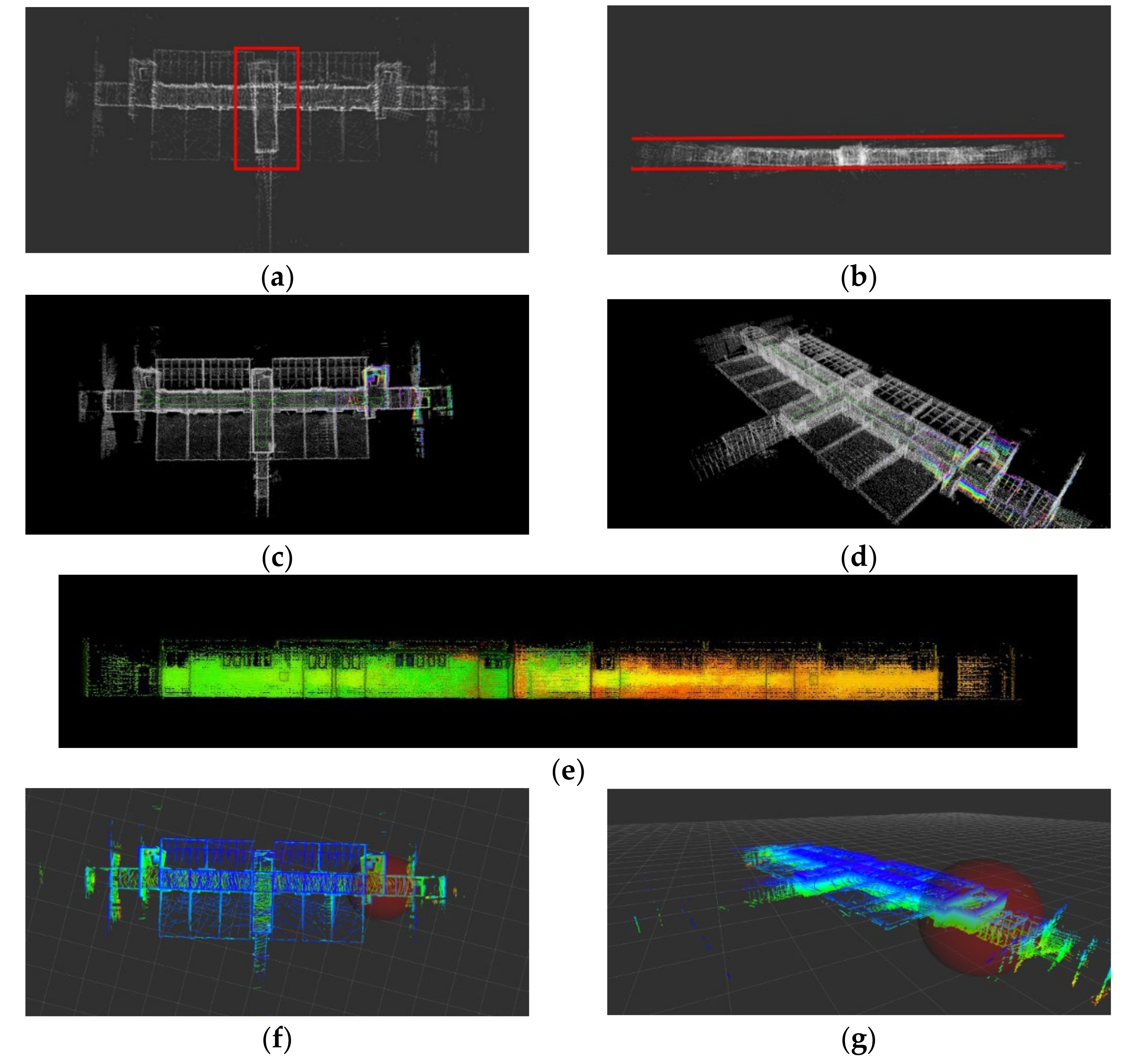
Measurements made in an environment consisting of a long corridor were processed with LOAM, A-LOAM, and HDL Graph SLAM algorithms, and the resulting maps are given in Figure 2.

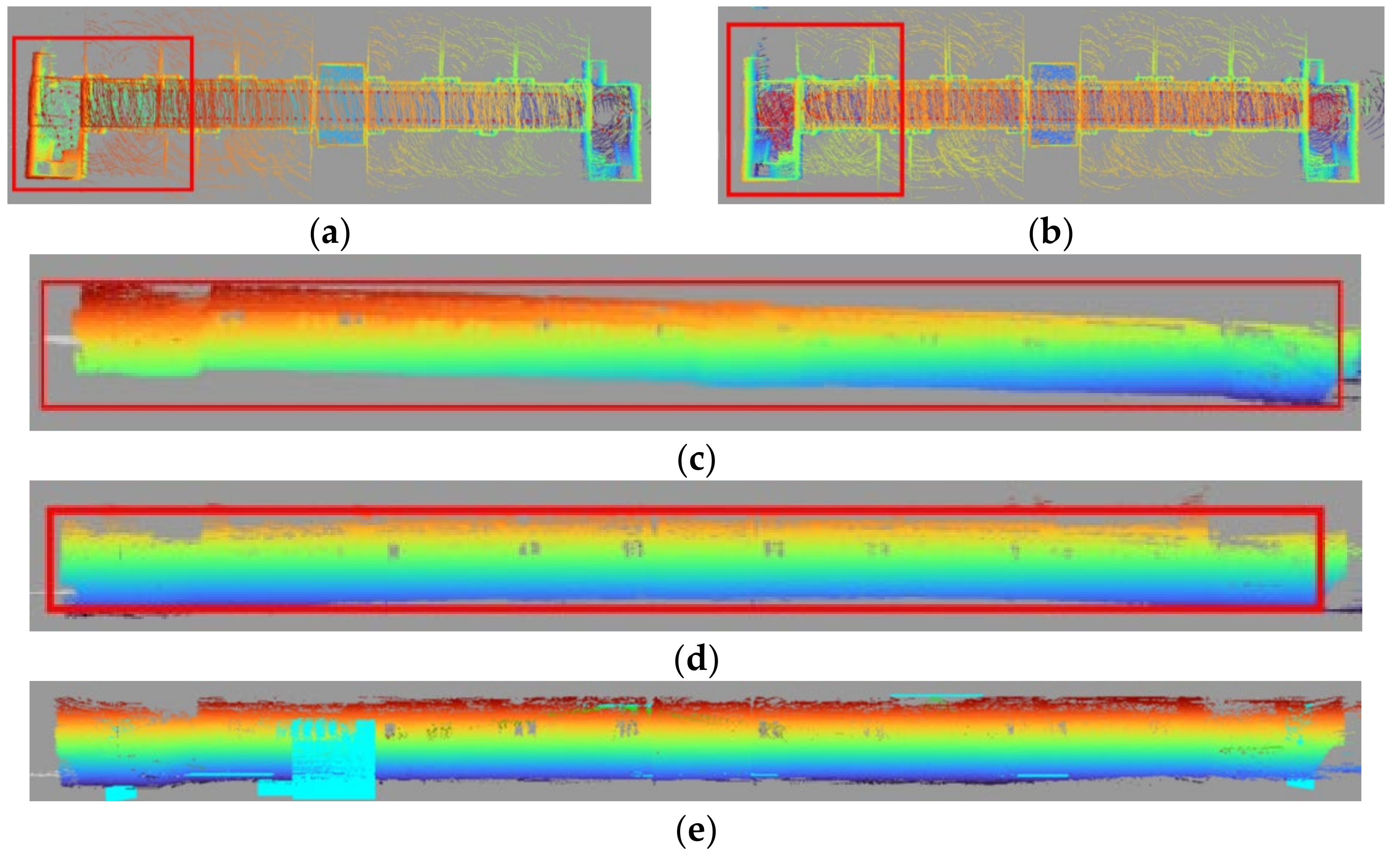
When the results of the LOAM algorithm given in Figure 2a,b are examined, there are significant odometry drifts in some regions in the long corridor environment. The deformation in the rectangular area marked in red in Figure 2a is caused by odometry drift. The red lines in Figure 2b represent the horizontal plane. Deviations from the horizontal plane are caused by odometry drift. The results of the A-LOAM algorithm given in Figure 2c–e are consistent with the LOAM algorithm, and no odometry drift is detected in the 3D point cloud. In the HDL Graph SLAM results given in Figure 2f,g, a minor odometry drift is detected in the middle section of the long corridor.

3.2. Experiments in Staircase

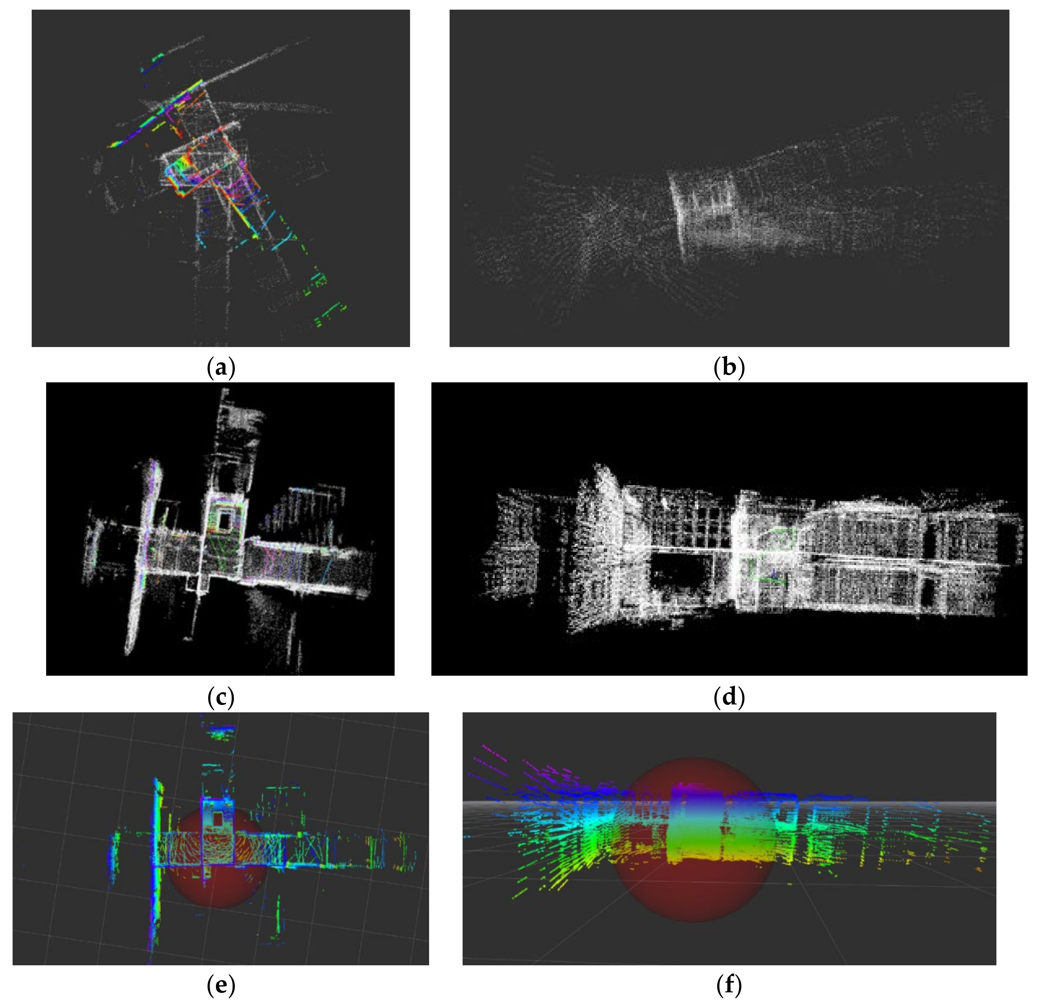
In order to determine the performance of SLAM algorithms in narrow spaces such as stairs, tests were carried out in the staircase environment with three different algorithms, and the results are given in Figure 3.

The results given in Figure 3a,b show that the LOAM algorithm has a very high odometry drift in the staircase environment. This caused distortions in the 3D map. A minimal amount of odometry drift was detected for the staircase environment in the A-LOAM results given in Figure 3c,d. No odometry drift was observed in the HDL Graph SLAM results given in Figure 3e,f. Thus, the HDL Graph SLAM algorithm gives more accurate results than other algorithms in the staircase environment.

3.3. Experiments in Outdoor Environment

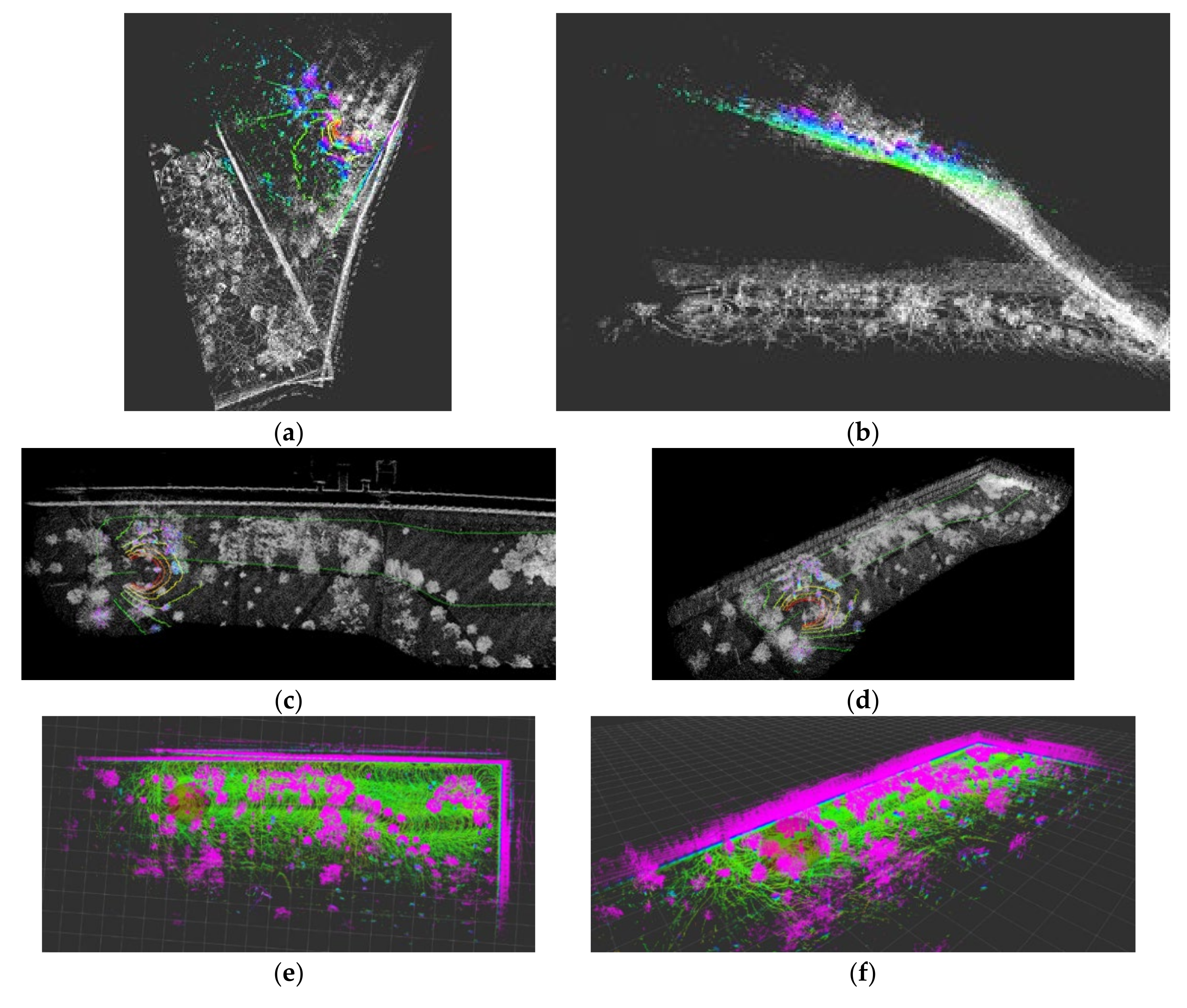
Within the scope of this study, the final tests were carried out in the outdoor environment, and the resulting maps of the LOAM, A-LOAM and HDL Graph SLAM algorithms are given in Figure 4.

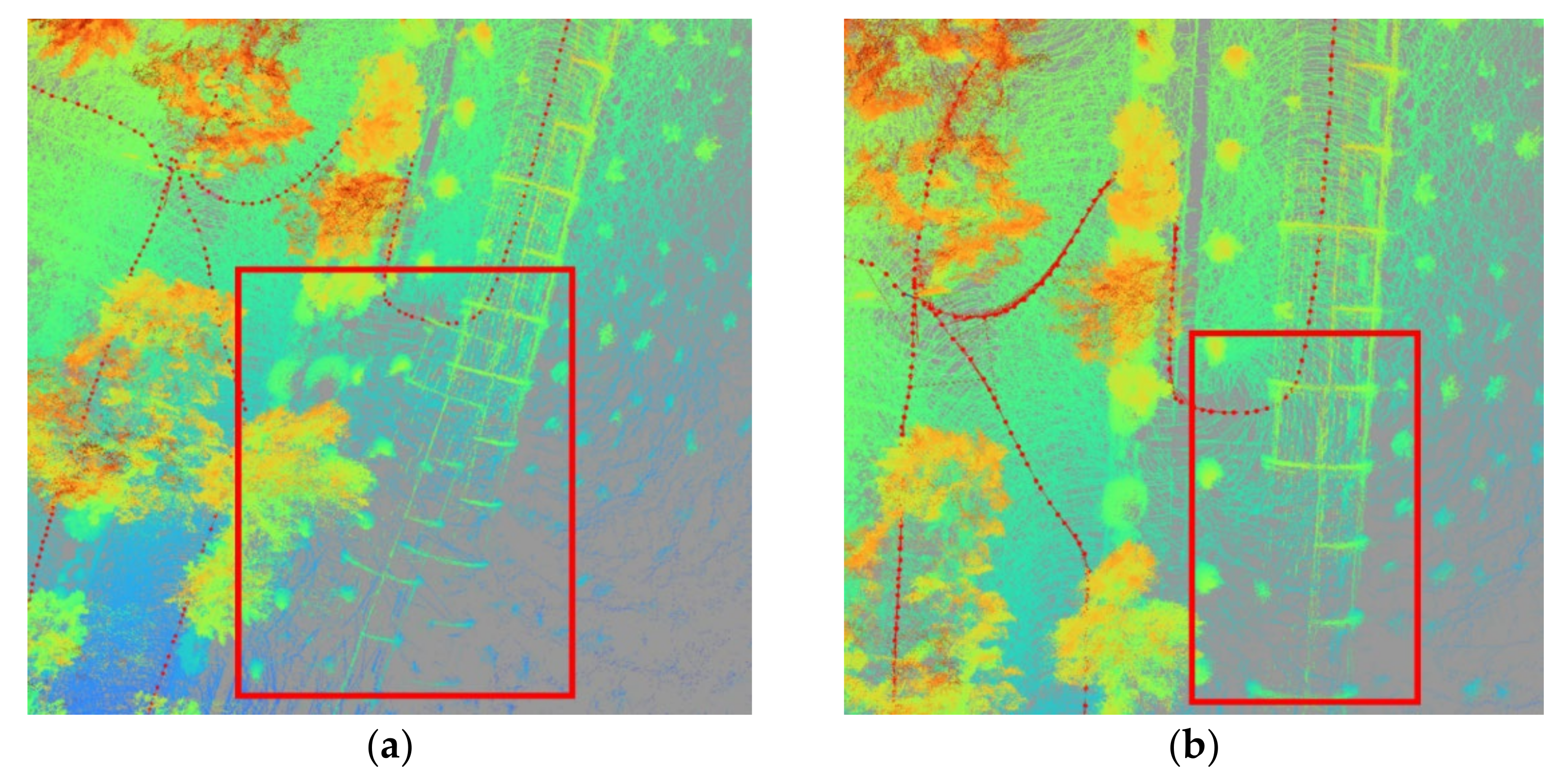
When the LOAM results given in Figure 4a,b are examined, it can be seen that there are significant drifts in the odometry and Z axis in regions with dense trees. According to the A-LOAM results given in Figure 4c,d, there is a curve in the long building walls due to the odometry drift. In the HDL Graph SLAM results given in Figure 4e,f, deformation is observed on the long building wall because of the odometry drift.

When all the results are examined, it is seen that the LOAM algorithm achieves partially satisfactory results. However, with an insufficient processing capacity of the computer, the data loss occurs in point clouds, causing odometry drifts. Because the processing capacity of the computer used in this study was not high enough, and because of the optimization problems of the LOAM algorithm, the odometry drifts have occurred in all point clouds in this study. More accurate results are obtained with the A-LOAM and HDL Graph SLAM algorithms than with the LOAM.

3.4. Loop Closure and Plane Detection

In this section, loop closure and plane detection methods of the interactive SLAM algorithm are applied to the results of A-LOAM and HDL Graph SLAM, and the effects of these methods are investigated. Although loop closure and plane detection methods were applied to both A-LOAM and HDL Graph SLAM results in this study, only A-LOAM results are shown in the figures below. The accuracies of both algorithms are given in the Results and Conclusions section.

Figure 5a shows the section with odometry drift in the outdoor environment. The point cloud corrected by the manual loop closure method is given in Figure 5b.

Figure 6 shows the top and side views of the point cloud with odometry drift in the indoor environment and the point clouds corrected by the automatic loop closure method.

In Figure 6c, the drift occurring predominantly in the direction of the Z-axis can be seen. Figure 6d shows that the drift in the Z direction is substantially eliminated with the automatic loop closure method, but there is a curve, especially in the middle section. It is believed that this error, which occurs mainly in the long corridor environment, can be eliminated by applying the plane detection method after the automatic loop closure method. Figure 6e is a side view of the corrected point clouds, following the ground and plane detection.

When the results are examined, it is seen that the curvature of the ground after the automatic loop closure algorithm is corrected by plane detection. In addition, since the perpendicularity was defined between the floors and the corridor, irregularities on the walls were corrected.

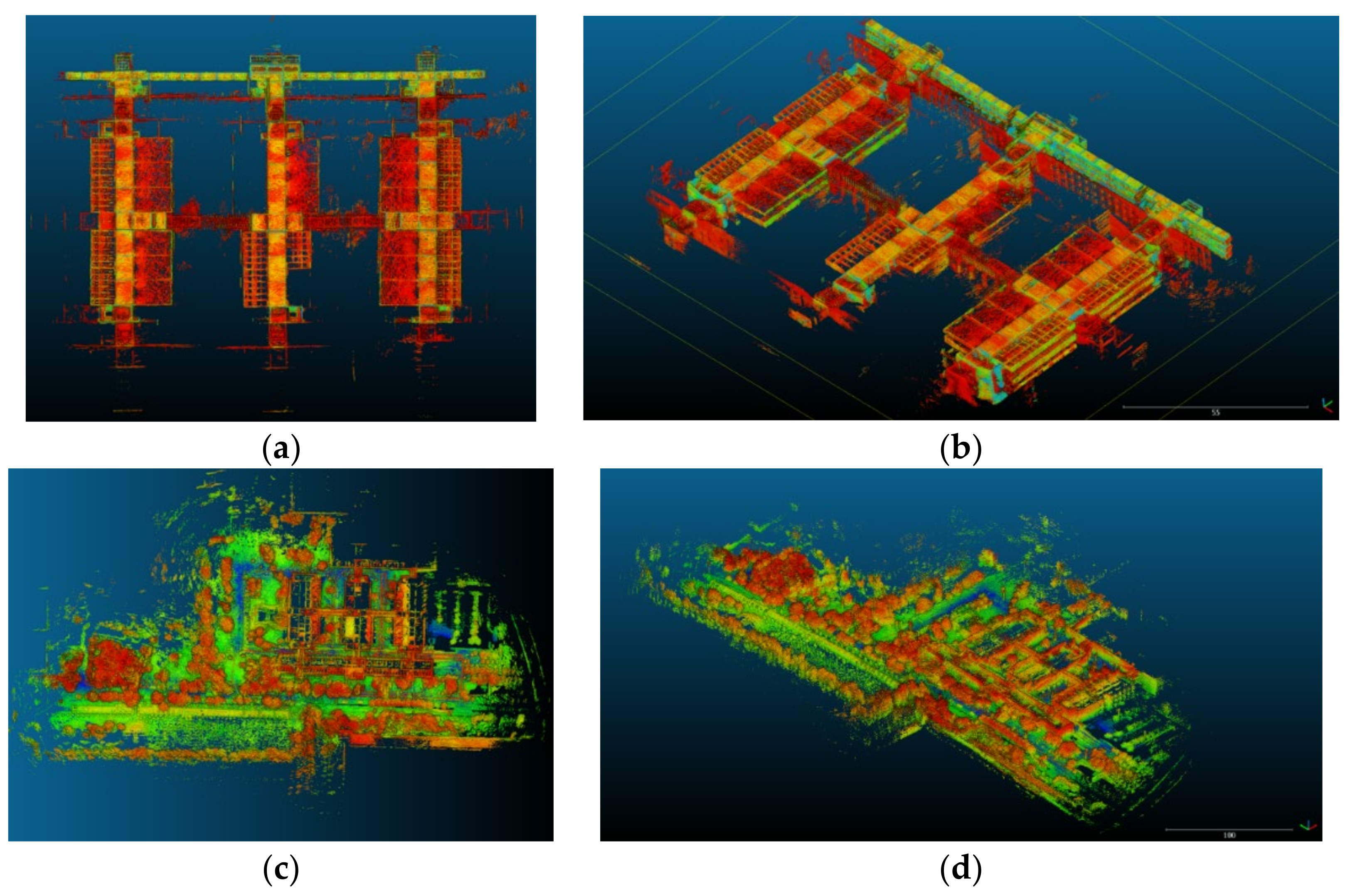
Top and perspective views of the corrected final 3D maps of the indoor and outdoor environments are in Figure 7.

4. Results and Conclusions

In this study, to determine the accuracies of the A-LOAM and HDL Graph SLAM algorithms, the distances obtained in the final 3D maps were compared with their actual values, and the results are given in

Table 1. Differences between the actual values and the SLAM Results for indoor environment.

Actual Value (m)	A-LOAM Result (m)	HDL Graph SLAM Result (m)	A-LOAM Error (cm)	HDL Graph SLAM Error (cm)
60.476	60.458	60.381	−1.8	−9.5
13.945	13.983	13.909	3.8	−3.6
8.262	8.249	8.304	−1.3	4.2
4.081	4.108	4.128	2.7	4.7
1.705	1.712	1.713	0.7	0.8
1.592	1.623	1.649	3.1	5.7
1.279	1.272	1.232	−0.7	−4.7
1.263	1.254	1.239	−0.9	−2.4

and

Table 2. Differences between the actual values and the SLAM Results for an outdoor environment.

Actual Value (m)	A-LOAM Result (m)	HDL Graph SLAM Result (m)	A-LOAM Error (cm)	HDL Graph SLAM Error (cm)
98.643	98.628	98.701	−1.5	5.8
75.164	75.141	75.115	−2.3	−4.9
40.487	40.503	40.529	1.6	4.2
12.762	12.786	12.734	2.4	−2.8
3.267	3.252	3.242	−1.5	−2.5
1.452	1.443	1.487	−0.9	3.5
0.408	0.419	0.435	1.1	2.7

for indoor and outdoor environments respectively. Actual values refer to direct on-site measurement results.

In

Table 3. Accuracies of the Algorithms.

	A-LOAM		HDL Graph SLAM
	Indoor	Outdoor	Indoor	Outdoor
Mean Error (cm)	1.9	1.6	4.0	3.8
Standard Deviation (cm)	2.1	1.8	5.0	4.2

, mean error and standard deviation values of the results are given, indicating that the accuracy of the A-LOAM results is two times more accurate than HDL Graph SLAM results.

This study aimed to test the performances of different SLAM algorithms in 3D mapping studies in indoor and outdoor environments. Test results show that the LOAM algorithm was less accurate than the A-LOAM and HDL Graph SLAM algorithms in both indoor and outdoor environments. However, the LOAM algorithm may give better results with more powerful computer hardware. The processing times of both the A-LOAM and HDL Graph SLAM algorithms are approximately equal, depending on the size and level of detail in the studied area. However, in order to obtain high accuracy results with the LOAM algorithm, it is recommended that the processor capacity of the computer used should be at least Intel i7 or equivalent.

In addition, loop closure and plane detection methods were applied to the 3D maps obtained with A-LOAM and HDL Graph SLAM algorithms. It has been determined that the odometry drift, which occurred especially on long lines and long corridor environments, can be largely eliminated by manual and automatic loop closure methods. Also, it has been determined that the plane detection method after the automatic loop closure method improves the results significantly, especially in indoor environments.

Additional sensors such as IMU and GNSS were not used in this study. The SLAM algorithms could provide more accurate results with additional sensors; therefore, further studies should be conducted to evaluate these possibilities. In addition, the Velodyne VLP-16 LIDAR sensor was used in the mobile mapping system in the study. By increasing the number of sensors to 2, more points related to the measured environment will be included in the SLAM algorithms, and the resulting 3D map will be more accurate.