
An Item Retrieval Algorithm in Flexible High-Density Puzzle Storage Systems

Abstract
1. Introduction
2. Related Literature
3. Methodology
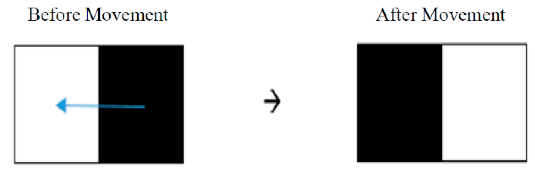
3.1. Network Elements
3.2. Retrieval Scenarios
3.2.1. Assigning White Cells to Specific Areas of the Puzzle
3.2.2. At Least One Empty Cell in Each Column and Row
3.2.3. Assigning a White Cell Specifically to Each Requested Item
3.2.4. Assigning a White Cell to a Called Item Based on the Nearest Distance
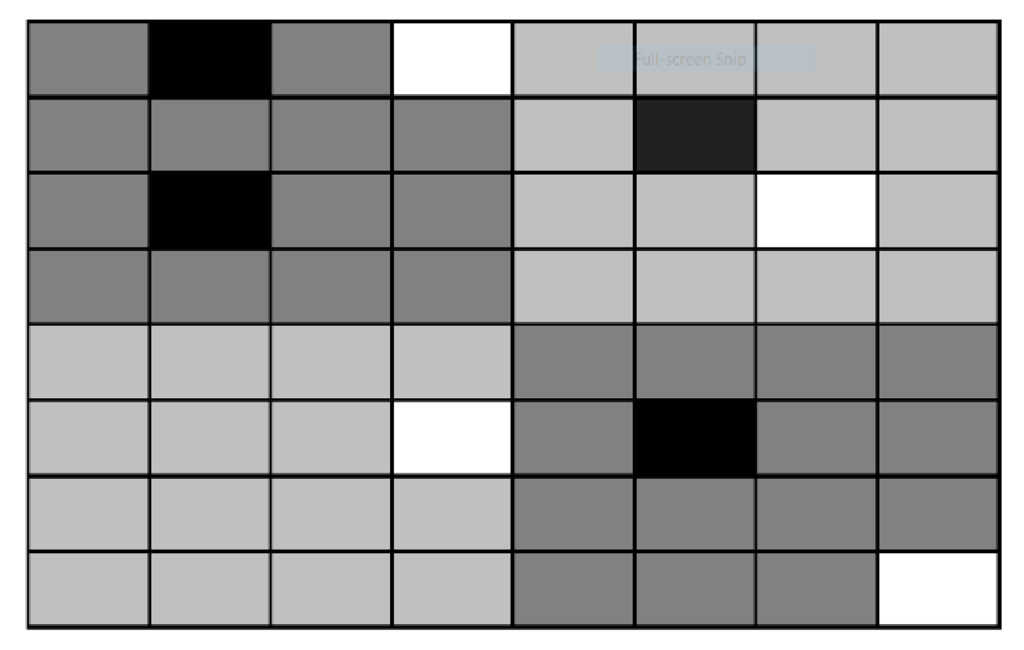
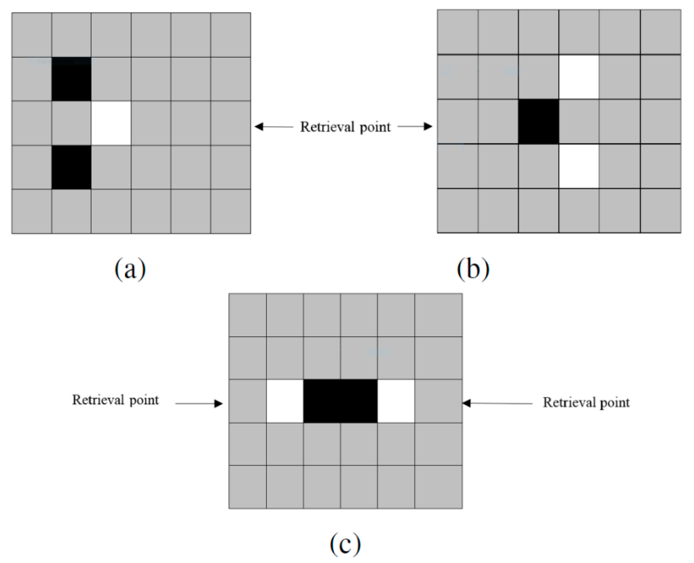
3.3. Puzzle Setup
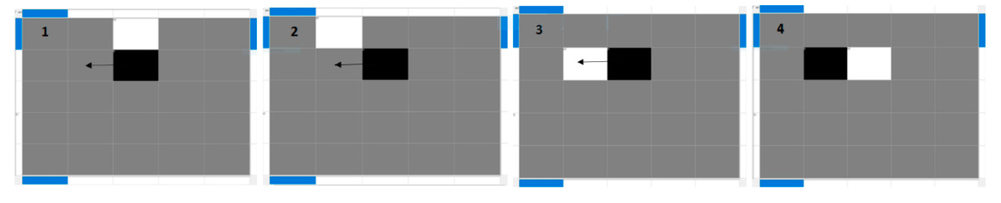
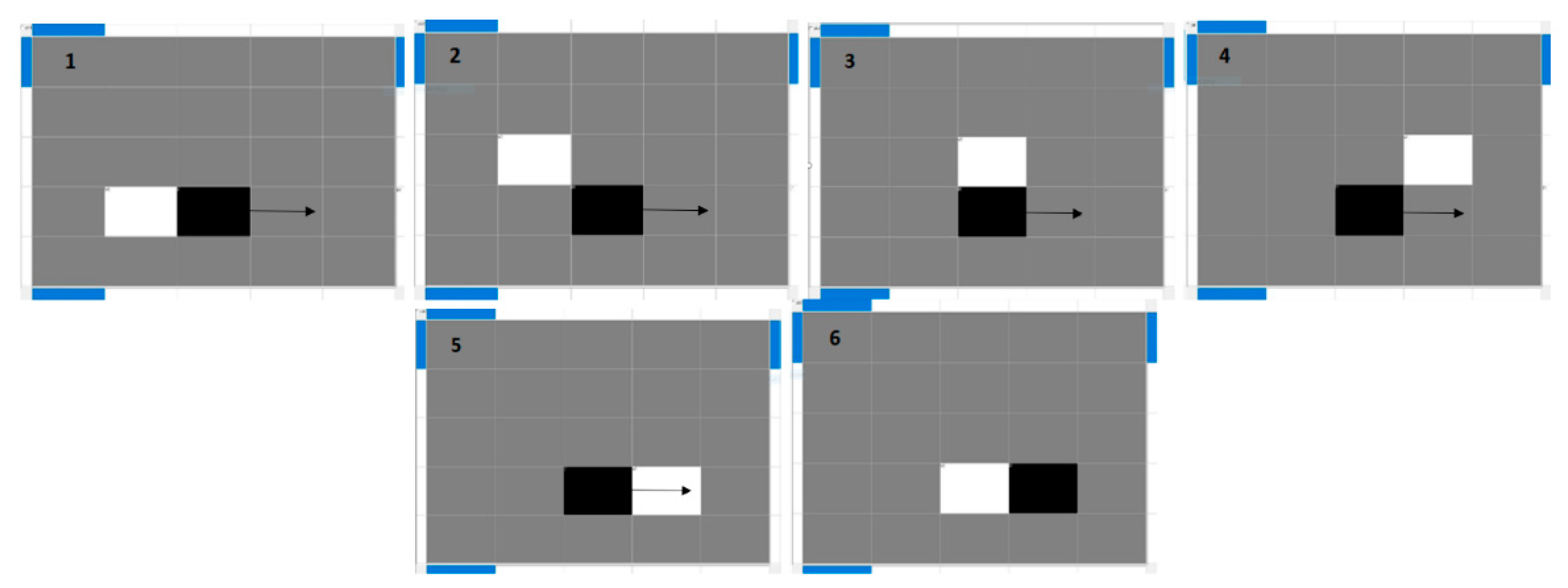
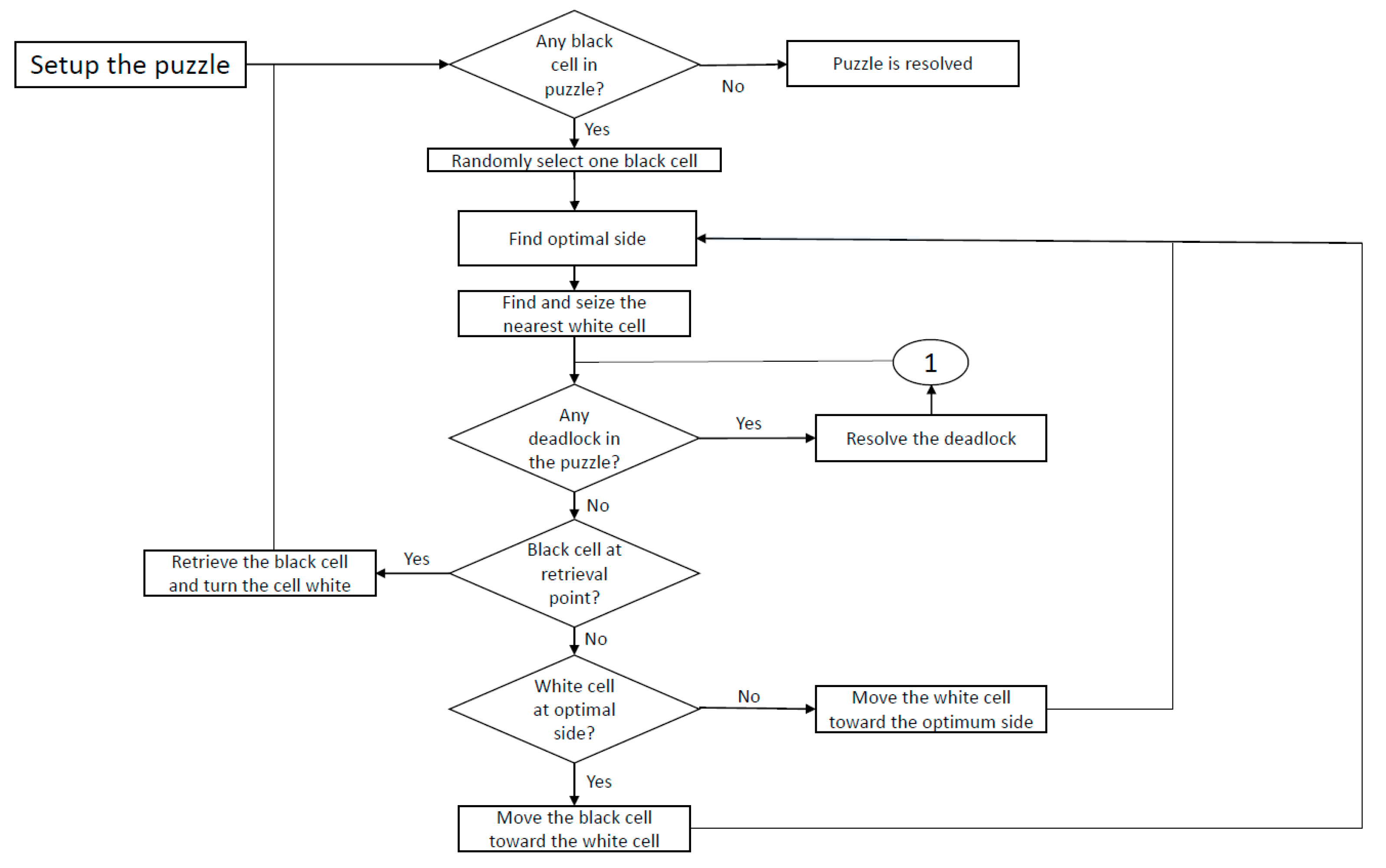
3.4. Algorithm
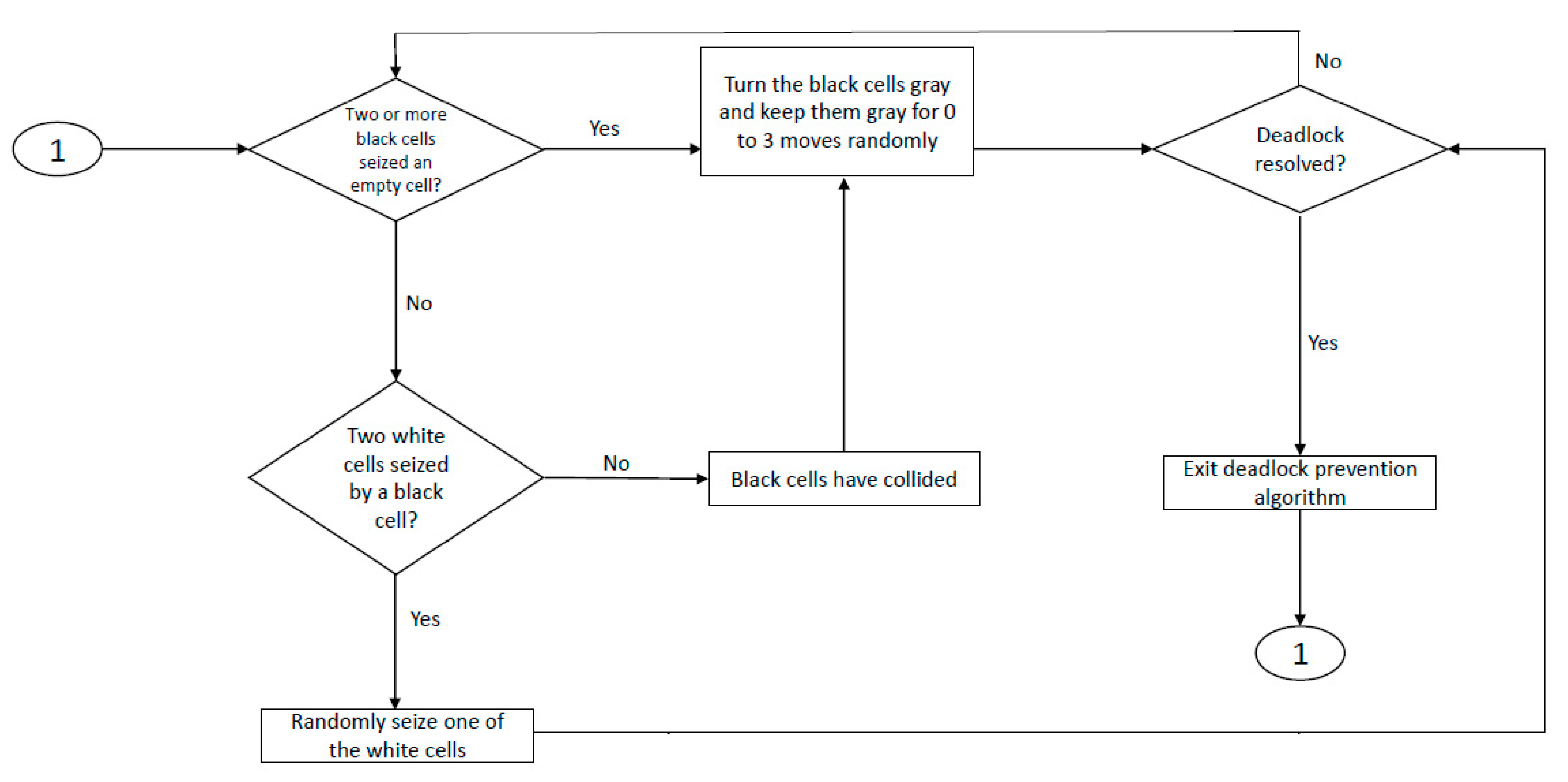
3.4.1. Deadlock Prevention
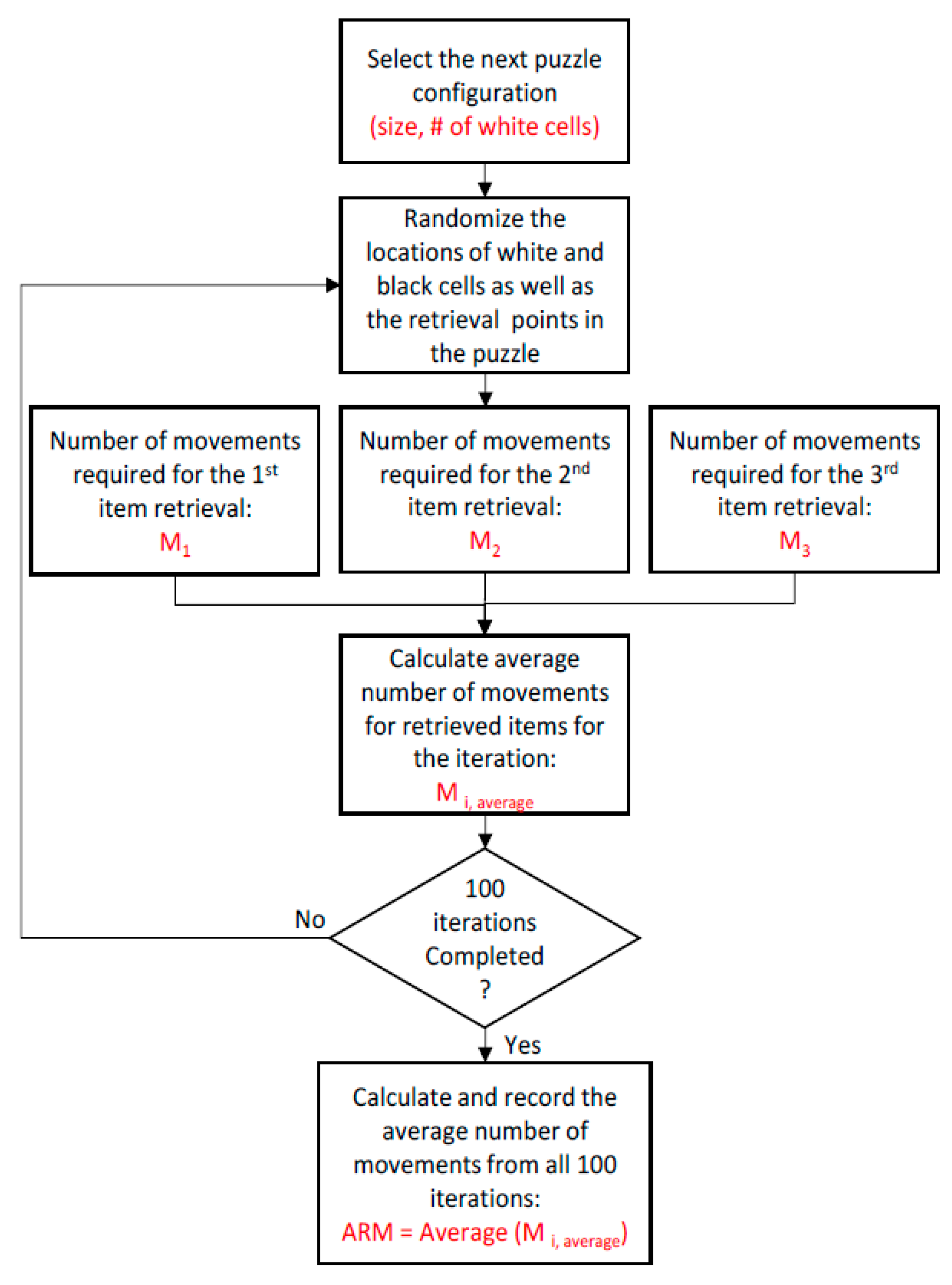
3.4.2. Methodology Flowcharts
3.4.3. The Novelty Aspects of the Present Algorithm
- We considered a deadlock prevention algorithm in our main algorithm. This prevents the algorithm to stick in deadlock situations. Therefore, our algorithm always results in a solution.
- Our high-density puzzle algorithm is capable of retrieving items from all sides of the puzzle. This increases the flexibility of our storage system and improves the average retrieval movements (ARM) needed to retrieve the items.
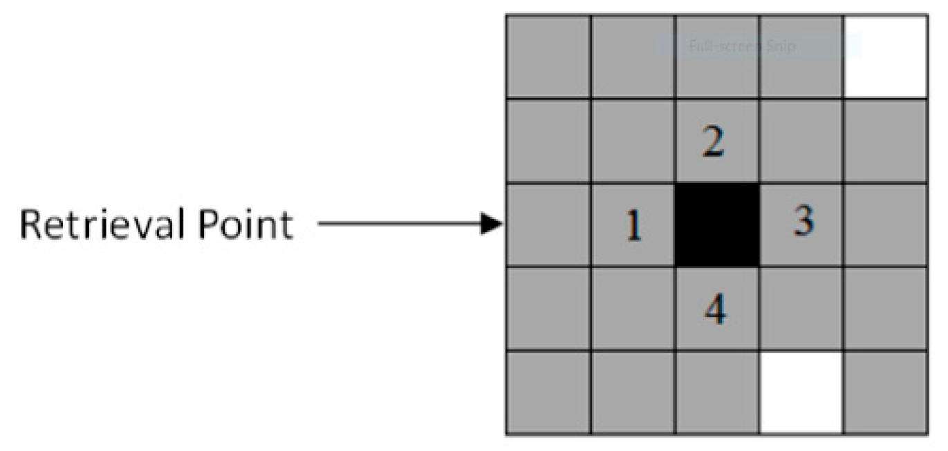
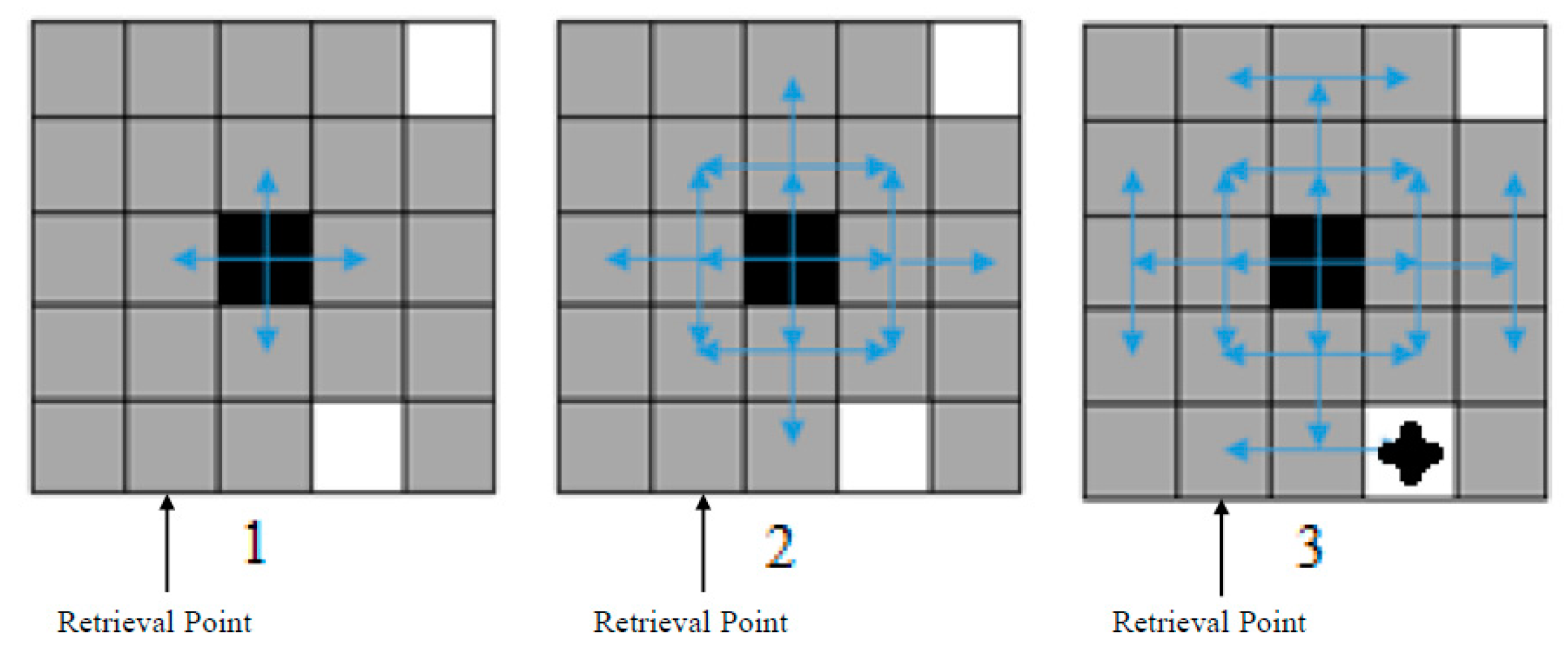
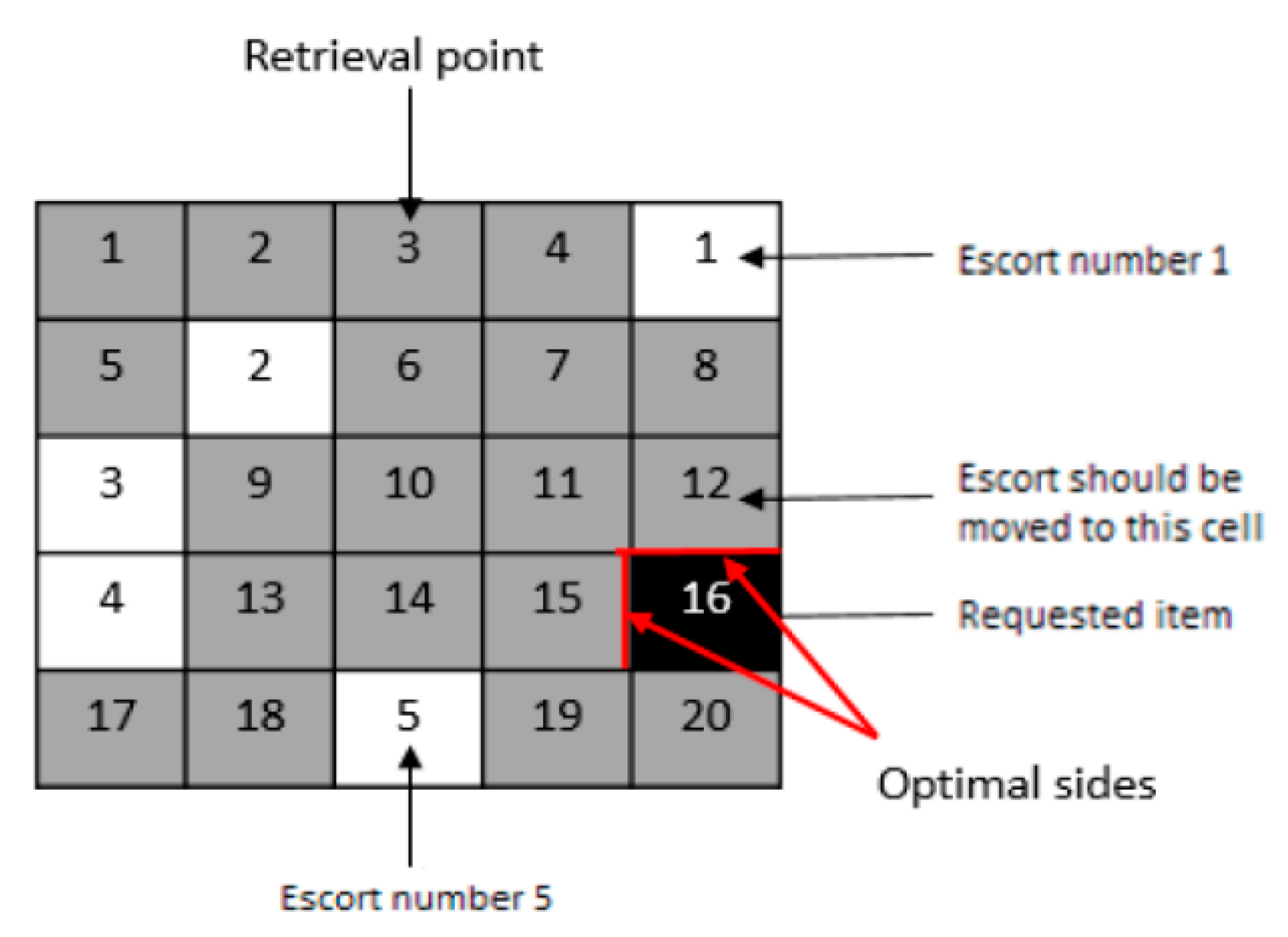
- We introduced a novel search algorithm which works based on sending a message to all four directions of the black cell to seize a white cell. If the algorithm cannot find a white cell next to the black cell, each cell which has received the message sends it to three different directions to find an empty spot. The main advantage that our search algorithm provides is decreasing ARM by finding the nearest empty spot to the requested item.
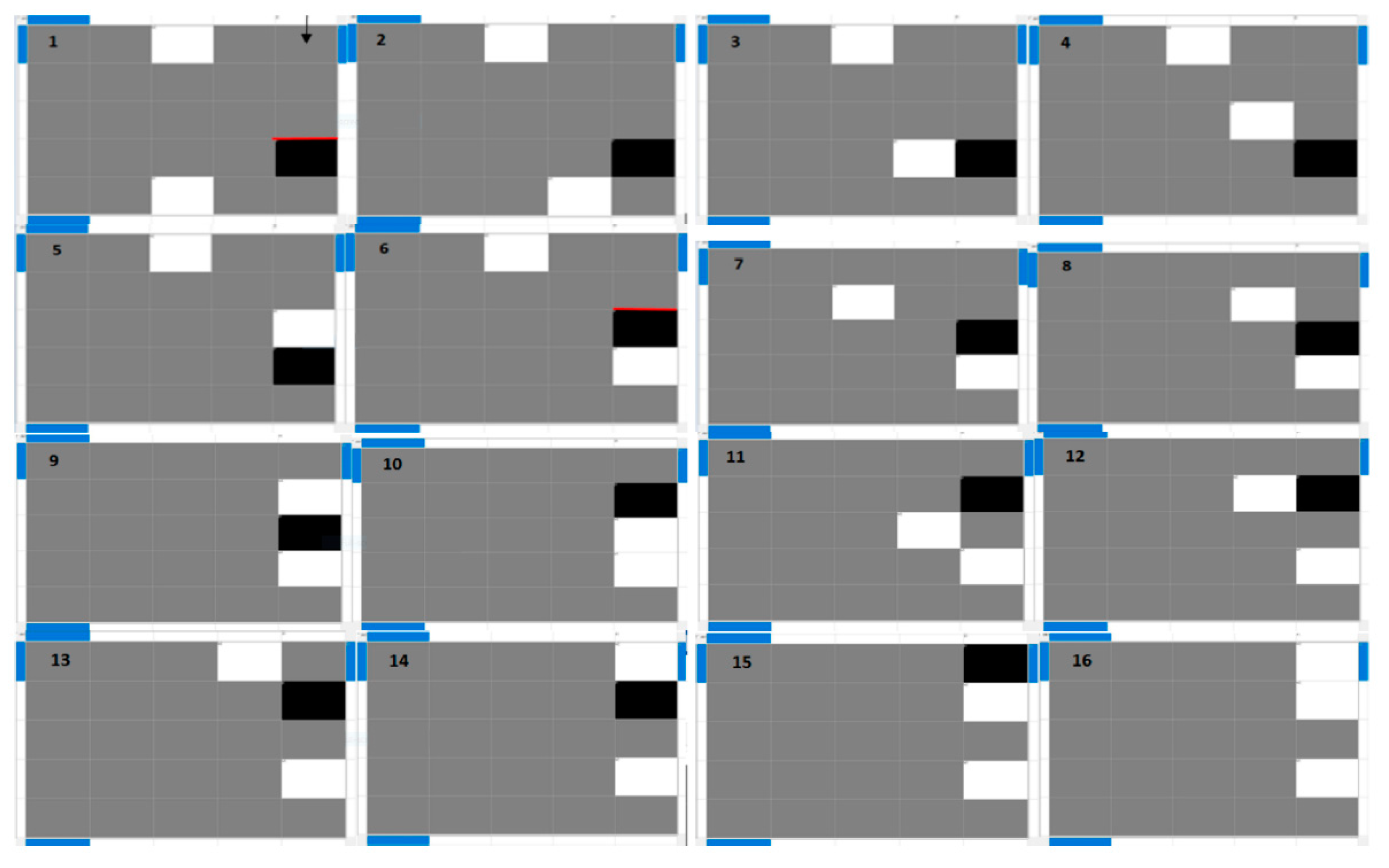
3.5. Examples
3.5.1. Example 1
3.5.2. Example 2
4. Analysis and Results
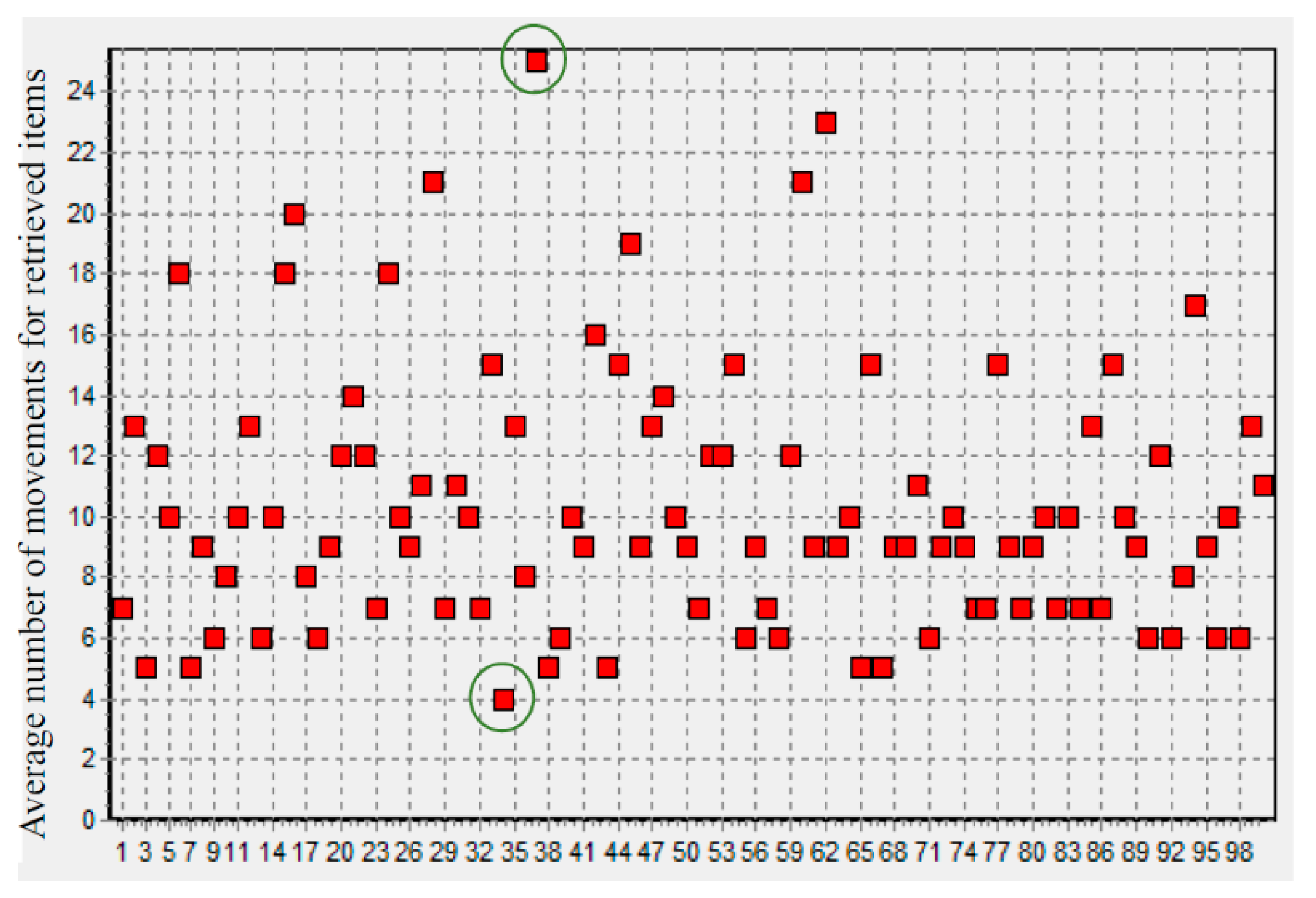
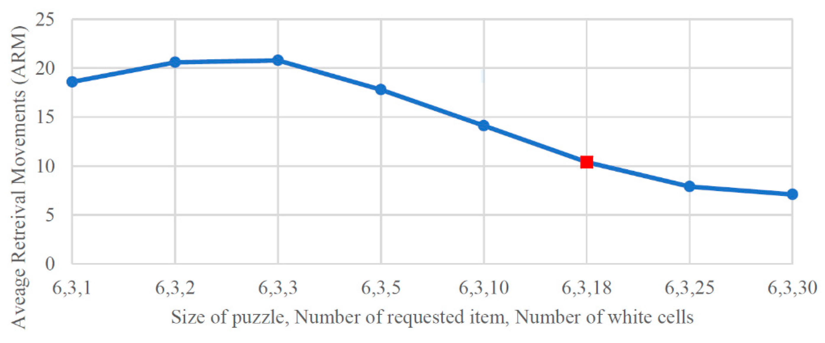
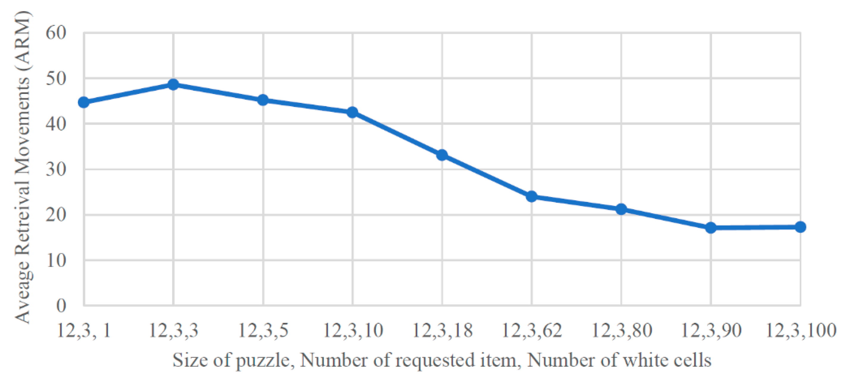
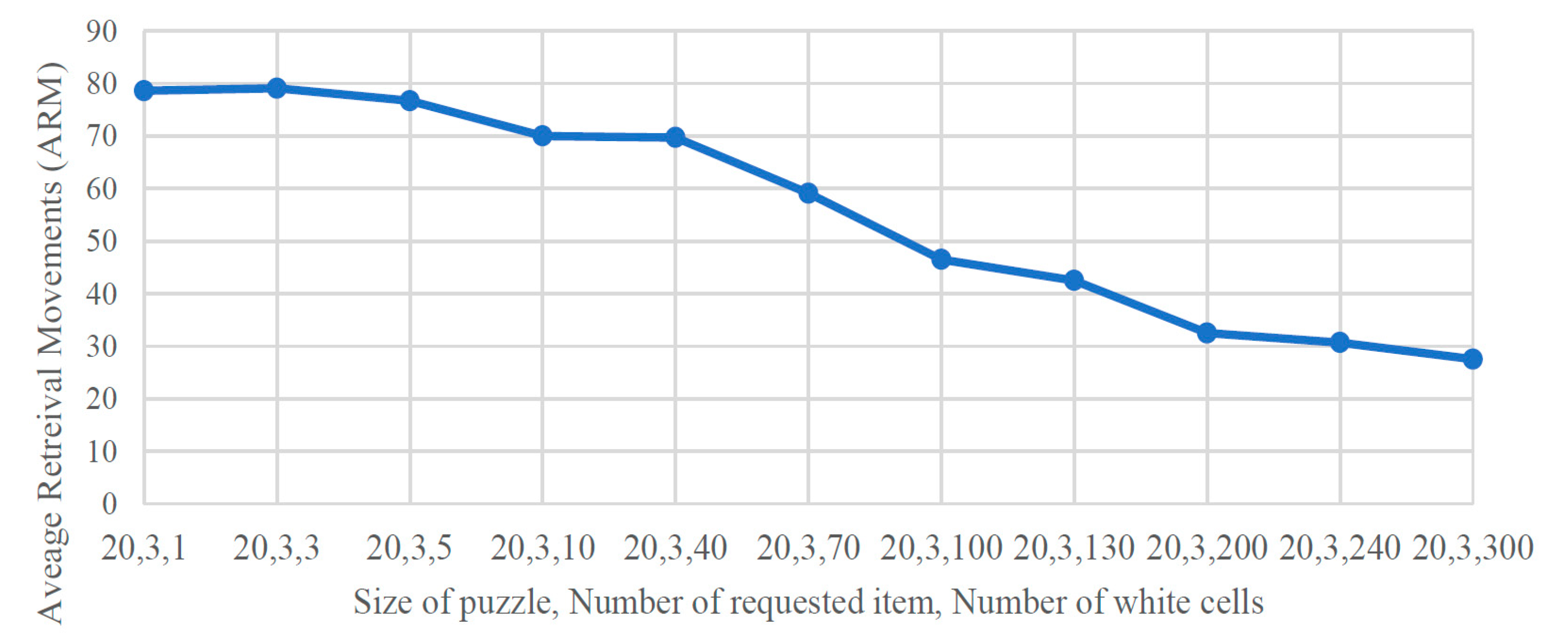
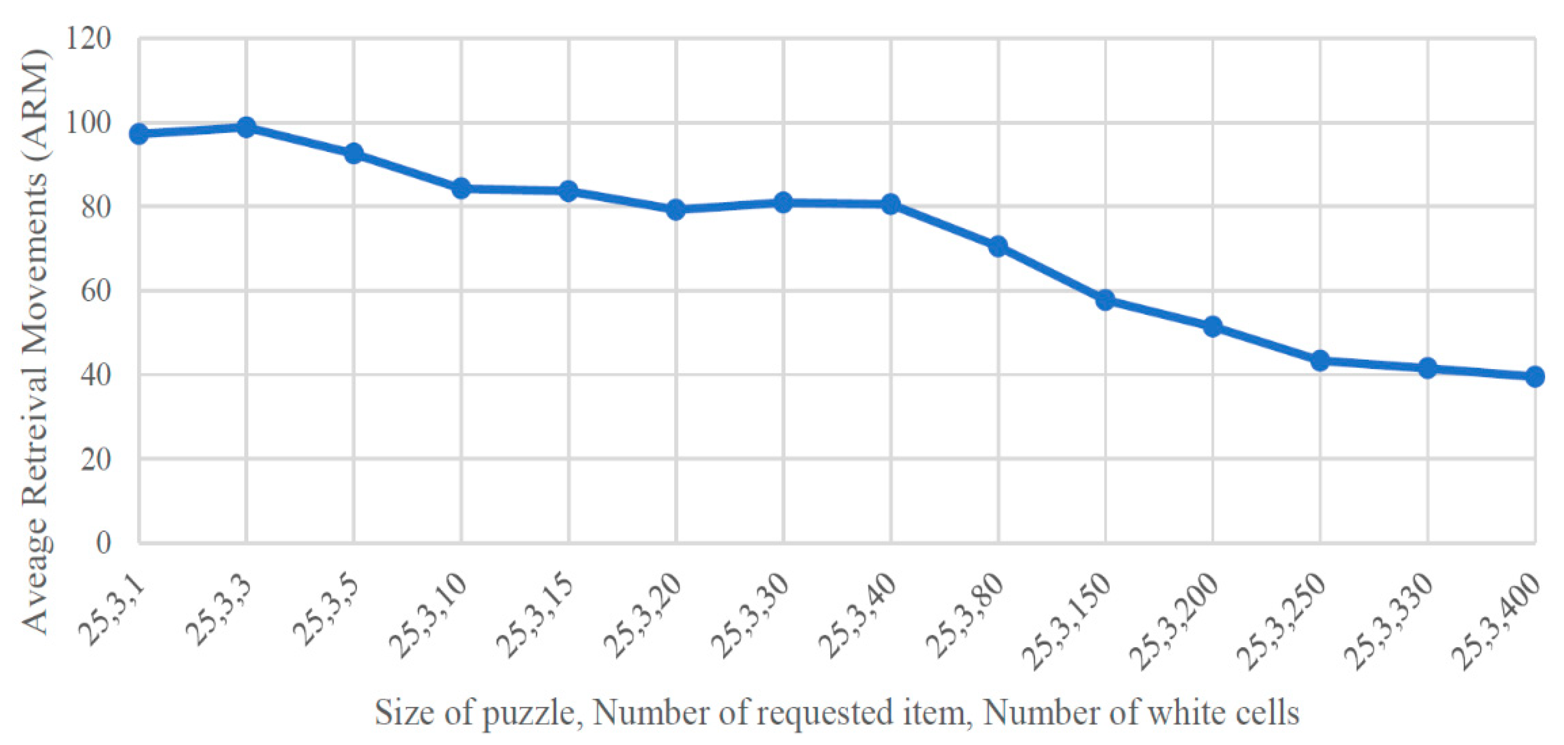
4.1. Simulation Results
- Options Effect: increasing the number of white cells increases the options that the black cell has for seizing the nearest white cell;
- Deadlock Effect: increasing the number of white cells increases the possibility of reaching a deadlock.
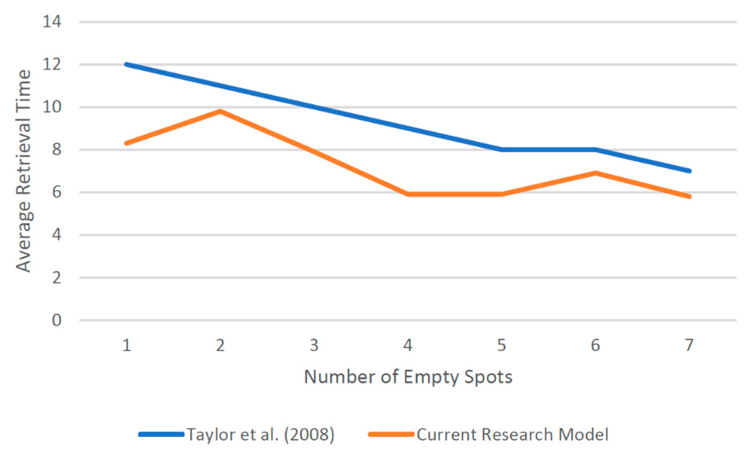
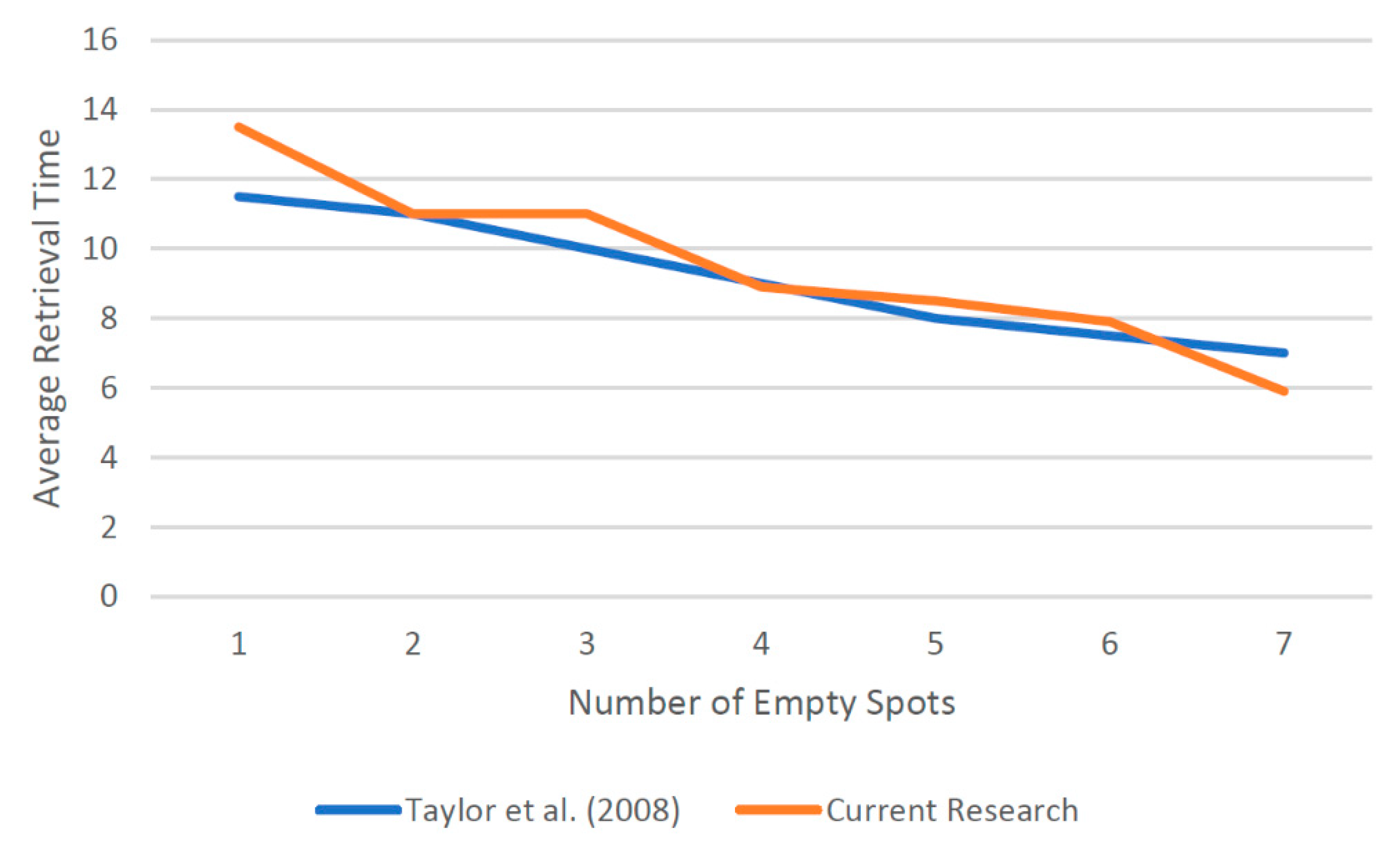
4.2. Comparison of Our Algorithm with Previous Studies
5. Conclusions
- Including a deadlock prevention algorithm into our main algorithm;
- Retrieving items from all sides of the puzzle;
- Introducing a new search algorithm to find the nearest empty cell to the requested item.
Author Contributions
Funding
Institutional Review Board Statement
Informed Consent Statement
Data Availability Statement
Conflicts of Interest
References
- Srinivas, S.S.; Marathe, R.R. Moving towards “mobile warehouse”: Last-mile logistics during COVID-19 and beyond. Transp. Res. Interdiscip. Perspect. 2021, 10, 100339. [Google Scholar]
- Seibold, Z.; Stoll, T.; Furmans, K. Layout-optimized sorting of goods with decentralized controlled conveying modules. In Proceedings of the 2013 IEEE International Systems Conference (SysCon), Orlando, FL, USA, 15–18 April 2013. [Google Scholar]
- Gue, K.R. Very high density storage systems. IIE Trans. 2006, 38, 79–90. [Google Scholar] [CrossRef]
- Gue, K.R.; Furmans, K.; Seibold, Z.; Uludağ, O. GridStore: A puzzle-based storage system with decentralized control. IEEE Trans. Autom. Sci. Eng. 2013, 11, 429–438. [Google Scholar] [CrossRef]
- Hearn, R.A.; Demaine, E.D. PSPACE-completeness of sliding-block puzzles and other problems through the nondeterministic constraint logic model of computation. Theor. Comput. Sci. 2005, 343, 72–96. [Google Scholar] [CrossRef]
- Gue, K.R.; Kim, B.S. Puzzle-based storage systems. Nav. Res. Logist. 2007, 54, 556–567. [Google Scholar] [CrossRef]
- Gue, K.R.; Furmans, K. Decentralized control in a grid-based storage system. In IIE Annual Conference Proceedings; Institute of Industrial and Systems Engineers (IISE): Peachtree Corners, GA, USA, 2011; p. 1. [Google Scholar]
- Rohit, K.V.; Taylor, G.D.; Gue, K.R. Retrieval Time Performance in Puzzle-Based Storage Systems. In IIE Annual Conference Proceedings; Institute of Industrial and Systems Engineers (IISE): Peachtree Corners, GA, USA, 2010; p. 1. [Google Scholar]
- Gue, K.R.; Uludag, O.; Furmans, K. A high-density system for carton sequencing. In Proceedings of the International Material Handling Research Colloquium 2012, Gardanne, France, 25–28 June 2012. [Google Scholar]
- Furmans, K.; Gue, K.R.; Seibold, Z. Optimization of failure behavior of a decentralized high-density 2D storage system. In Dynamics in Logistics; Springer: Berlin/Heidelberg, Germany, 2013; pp. 415–425. [Google Scholar]
- Uludag, O. GridPick: A High Density Puzzle Based Order Picking System with Decentralized Control. Ph.D. Thesis, Auburn University, Auburn, AL, USA, 9 January 2014. [Google Scholar]
- Krühn, T.; Sohrt, S.; Overmeyer, L. Mechanical feasibility and decentralized control algorithms of small-scale, multi-directional transport modules. Logist. Res. 2016, 9, 1–4. [Google Scholar] [CrossRef]
- Mirzaei, M.; De Koster, R.B.; Zaerpour, N. Modelling load retrievals in puzzle-based storage systems. Int. J. Prod. Res. 2017, 55, 6423–6435. [Google Scholar] [CrossRef]
- Hao, G. GridHub: A Grid-Based, High-Density Material Handling System. Ph.D. Thesis, University of Louisville, Louisville, KY, USA, May 2020. [Google Scholar]
- Shekari Ashgzari, M.; Gue, K.R. A puzzle-based material handling system for order picking. Int. Trans. Oper. Res. 2021, 28, 1821–1846. [Google Scholar] [CrossRef]
- Azadeh, K.; De Koster, R.; Roy, D. Robotized and automated warehouse systems: Review and recent developments. Transp. Sci. 2019, 53, 917–945. [Google Scholar] [CrossRef]
- Boysen, N.; De Koster, R.; Weidinger, F. Warehousing in the e-commerce era: A survey. Eur. J. Oper. Res. 2019, 277, 396–411. [Google Scholar] [CrossRef]
- Kota, V.R.; Taylor, D.; Gue, K.R. Retrieval time performance in puzzle-based storage systems. J. Manuf. Technol. Manag. 2015, 26, 582–602. [Google Scholar] [CrossRef]
- Manzini, R.; Accorsi, R.; Gamberi, M.; Penazzi, S. Modeling class-based storage assignment over life cycle picking patterns. Int. J. Prod. Econ. 2015, 170, 790–800. [Google Scholar] [CrossRef]
- Seibold, Z. Logical Time for Decentralized Control of Material Handling Systems; KIT Scientific Publishing: Karlsruher, Germany, 2016. [Google Scholar]
- Yalcin, A.; Koberstein, A.; Schocke, K.O. An optimal and a heuristic algorithm for the single-item retrieval problem in puzzle-based storage systems with multiple escorts. Int. J. Prod. Res. 2019, 57, 143–165. [Google Scholar] [CrossRef]
- Zaerpour, N.; Yu, Y.; de Koster, R.B. Optimal two-class-based storage in a live-cube compact storage system. IISE Trans. 2017, 49, 653–668. [Google Scholar] [CrossRef]
- Taylor, G.D.; Gue, K.R. The effects of empty storage locations in puzzle-based storage systems. In IIE Annual Conference Proceedings; Institute of Industrial and Systems Engineers (IISE): Peachtree Corners, GA, USA, 2008; p. 519. [Google Scholar]


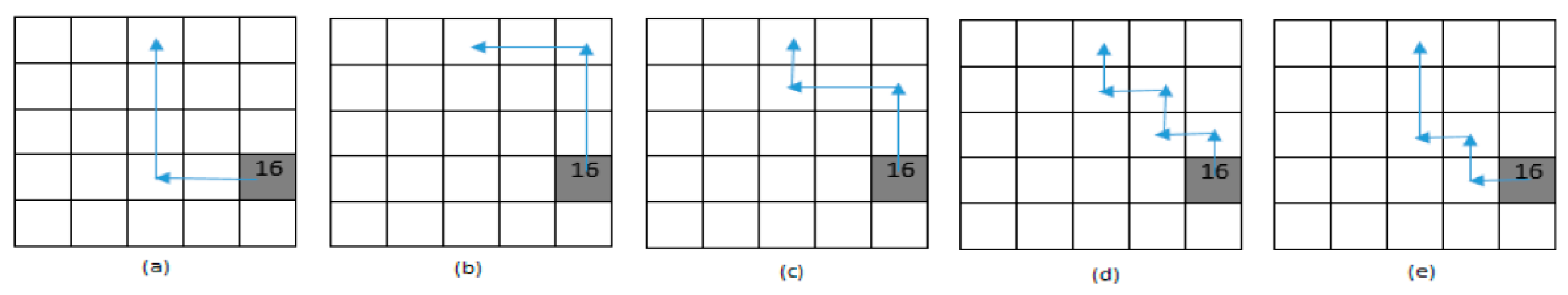
| Path | (a) | (b) | (c) | (d) | (e) |
|---|---|---|---|---|---|
| Number of movements with white cell number 1 | 23 | 21 | 19 | 15 | 19 |
| Number of movements with white cell number 5 | 21 | 19 | 21 | 17 | 17 |
| Case Number | Black Cell Location (i,j) | Mathematical Optimum Number of Movements | Software Program Simulation Results |
|---|---|---|---|
| 1 | 5,5 | 29 | 29 |
| 2 | 15,15 | 109 | 109 |
| 3 | 25,25 | 189 | 189 |
| 4 | 50,50 | 389 | 389 |
| 5 | 5,15 | 87 | 87 |
| 6 | 15,25 | 167 | 167 |
| 7 | 25,35 | 247 | 247 |
| 8 | 35,50 | 357 | 357 |
| 9 | 15,5 | 87 | 87 |
| 10 | 25,15 | 167 | 167 |
| 11 | 35,25 | 247 | 247 |
| 12 | 35,50 | 297 | 297 |
Publisher’s Note: MDPI stays neutral with regard to jurisdictional claims in published maps and institutional affiliations. |
© 2021 by the authors. Licensee MDPI, Basel, Switzerland. This article is an open access article distributed under the terms and conditions of the Creative Commons Attribution (CC BY) license (https://creativecommons.org/licenses/by/4.0/).
Share and Cite
Shirazi, E.; Zolghadr, M. An Item Retrieval Algorithm in Flexible High-Density Puzzle Storage Systems. Appl. Syst. Innov. 2021, 4, 38. https://doi.org/10.3390/asi4020038
Shirazi E, Zolghadr M. An Item Retrieval Algorithm in Flexible High-Density Puzzle Storage Systems. Applied System Innovation. 2021; 4(2):38. https://doi.org/10.3390/asi4020038
Chicago/Turabian StyleShirazi, Ehsan, and Mohammad Zolghadr. 2021. "An Item Retrieval Algorithm in Flexible High-Density Puzzle Storage Systems" Applied System Innovation 4, no. 2: 38. https://doi.org/10.3390/asi4020038
APA StyleShirazi, E., & Zolghadr, M. (2021). An Item Retrieval Algorithm in Flexible High-Density Puzzle Storage Systems. Applied System Innovation, 4(2), 38. https://doi.org/10.3390/asi4020038