Towards a More Robust Non-Rigid Robotic Joint

Abstract

The following paper presents an improved, low cost, non-rigid joint that can be used in both robotic manipulators and leg-based traction robotic systems. This joint is an improvement over the previous one presented by the same authors because it is more robust. The design iterations are presented and the final system has been modeled including some nonlinear blocks. A control architecture is proposed that allows compliant control to be used under adverse conditions or in uncontrolled environments. The presented joint is a cost-effective solution that can be used when normal rigid joints are not suitable.

1. Introduction

Robots are becoming increasingly present in daily tasks, both from a personal and an industrial point of view. The use of robots to assist in the execution of freight transport tasks in a factory plant and their use for the disinfection of common areas have increased significantly. To perform certain tasks, robots usually rely on manipulators that act like human arms and hands. In some cases, it is necessary for the traction system of a mobile robot to be more adaptable, and in these cases, locomotion systems similar to legs are used, such as those in [1].

In the above examples, movement or manipulation are common in unstructured environments. This means that these robot systems must be prepared for unexpected disturbances, such as rough terrain, external forces, collisions, etc. Collisions with obstacles or people and the risk of the robot breaking itself are particularly important, as the integrity of people and equipment are at risk. Considering that conventional robots are usually designed with rigid elements, a higher degree of sensor technology and better control are required to cope with external forces. In these applications, the use of flexible joints helps to improve safety for the people working in the vicinity of the robot system and also for the robots themselves, as the probability of breaking something decreases.

Despite the evolutionary effort for using flexible and more sophisticated solutions for the market [2,3,4,5,6,7], it is not yet very easy to find solutions in mature states with which to explore and perform experimental work, as Hoffman et al. [8] report. Even so, there are some works that should be mentioned, since they present varied solutions. The work from Wang et al. [9] is one of them, which resorts to a six degrees of freedom (DOF) fully parallel manipulator with elastic joints. The elastic component is used as the last link of an industrial manipulator and consists of three links connected by an elastic ball joint and a Hooke’s joint on each side. This joint is an example of a purely mechanical solution, but it does not have a damping effect on the system, which is very useful in the event of an impact, given its important characteristic.

A different solution was proposed by Yoneyama and Ito [10], which presents a flexible translational joint mechanism. The authors consider an adaptable adaptive joint with adjustable elasticity that can slide in multiple directions. The joint is built with servos that control the flexibility of a rubber band that locks into a ball bearing bed. Such joints are used as lower leg parts for a humanoid robot. Despite adding an elasticity component to the joint, this solution also does not have a damping component. Another characteristic of this joint is its variable elasticity, however it consumes energy for its control.

Kakogawa and Ma [11] have designed a fully passive elastic joint to be used on an inspection robotic vehicle. Each of the three links uses a spring, which can be different from each other, to introduce a torsional elasticity capability that allows the joints to be flexible even when the wheel is stopped. This joint also has no damping component, which could be an advantage for the use intended for this system.

Regarding the control of an elastic joint, there are some works that address it, from the 1980s to the present day [12,13,14,15,16,17,18], indicating that this issue is still an open line of research. Since the non-rigid joint increases the flexibility of the robot, the control methods must be adequate for the movement and permissiveness of such specific elastic joints.

The work from Zolo et al. [19] also stands out, since a compliance control for an anthropomorphic robot with elastic joints is used. It resorts to a PD plus gravity controller and the addition of a gravity-biased motor position variable. One thing that is anticipated by the control method is that, if the manipulator comes into contact with the environment, there are laws that achieve compliant behavior during this contact. The compliance control formulations have been tested experimentally.

An impedance control strategy is used by Ferretti et al. [20] in industrial manipulators to perform tasks where compliant position motion is required. This method focuses on creating a relation between errors in contact forces and position during a movement. The authors present a controller designed to use an impedance filter, as well as their experiments on a physical manipulator, which obtained relevant results.

Also applied to a robotic manipulator, Yin et al. [21] use a compliant control strategy for a single tendon-sheath actuator. The modeling and validation methods are presented, being performed experimentally. The model parameter identification is presented and the compliant control results are stated, even in the presence of collision detection, obtaining positive results.

In this paper, the design process for the next generation of the already existent non-rigid joint will be introduced, upgrading some aspects that were missing or needed in the previous version [22]. One difference in the developed joint from the above-mentioned works is the fact that a damping component has been added, which is useful in reducing high frequency oscillations, combined with the fact that it has been developed with passive components and therefore does not require energy consumption for achieving non-rigidity. The modeling process will also be presented, but will take into account the joint’s dead-zone, which is an interesting topic, as stated in recent works [23,24,25]. Furthermore, a more suitable control strategy is used and will be detailed. The experimental tests to model the joint and to validate the controllers will also be presented.

An introduction to the issues surrounding this work is presented in Section 1, while the joint design, proposed model and respective controls are presented in Section 2. Section 4 focuses on the experimental setup and the results obtained from the experiments performed. Finally, Section 5 presents the conclusions and possible ways forward for future work.

2. Design, Modeling and Control

As mentioned in Section 1, the work developed is an upgrade of an earlier work that has seen several improvements. The improved design, modeling and shared control are presented below. It should be noted that this development process has been done with low-cost parts, so the final system will have a very affordable price.

Throughout Section 2.1, several designs are presented, both in CAD and physically, the latter being 3D printed parts. It is important to present both figures because the CAD design has been idealized for 3D printing, this being completely different from other design technologies (namely CNC machining) and therefore requiring physical validation of the designed models.

2.1. Mechanical Design

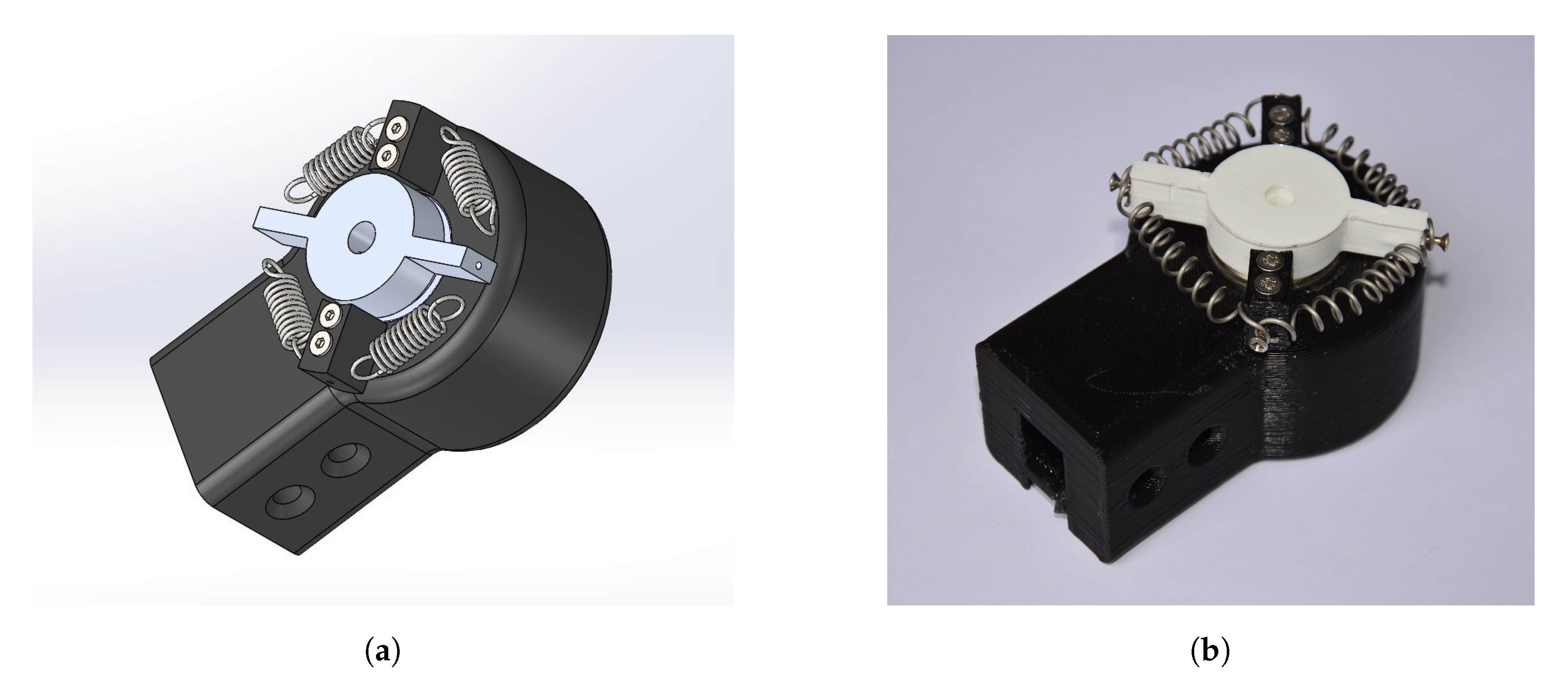
One of the main issues regarding the previous joint (v1), presented in Figure 1a,b, was its mechanical design, which is directly related to the mechanical robustness of the solution. The problems that were found in the previous version were as follows.

(a)

Spring support point—allowed springs to come out when they were not under tension;

(b)

Central part support—allowed central part to twist on the axis of rotation;

(c)

Springs ineffective—they became worn after extensive use since their position was too stretched;

(d)

Difficulty in assembling—given the structure and the required assembly, it was very difficult to assemble the joint;

(e)

Unstable structure—resulting in an increased deadzone effect of the joint;

(f)

Low chance of spring variation—the configuration had a small range of available springs to change its forces and sizes;

(g)

Low stiffness—the resulting stiffness of the joint was not hard enough, compared to the desired one.

Having these problems in mind, there were several versions between the previous one and the last one presented in the paper. The second version of the joint used two spiral springs attached to a central support, which could introduce an elastic component into the axis of rotation. This presented solution solved problems (a) and (c), but could not solve the rest. For point (f) this solution proved to be even worse because there were no different types of spiral spring. Some 3D-printed spring solutions were tried, but failed terribly because plastic materials easily deform, lose their elasticity and then break.

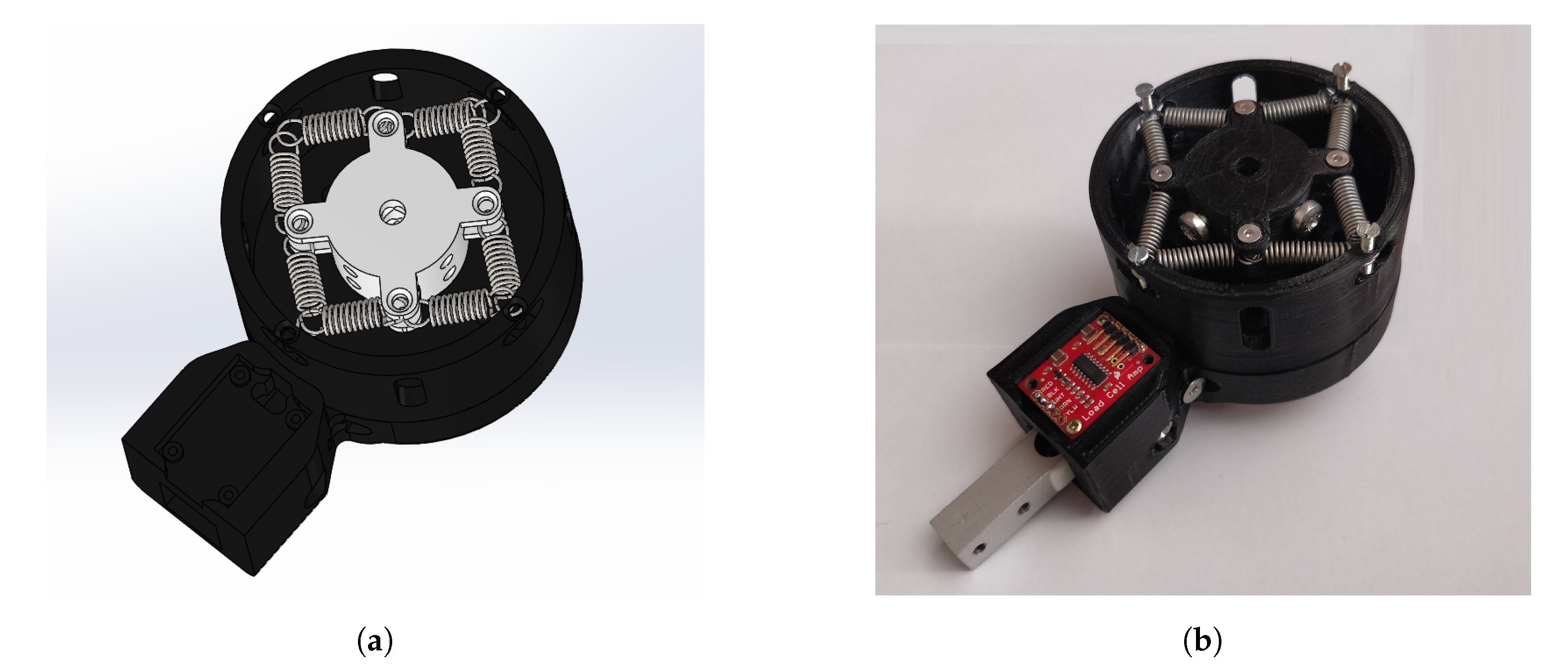
Considering that solutions with steel springs are more robust than those printed on plastic material, we decided to find another solution for coupling to the joint. A new version (v5) was developed and is a solution that is extremely robust and modular, it is very easy to assemble and disassemble, its strength can easily be changed by simply replacing the springs, and the only question left is whether the springs will be deformed after some time (problem (c)). However, after extensive tests with the springs used, it was found that they do not display significant deformation.

Although this is a very promising solution, during the control implementation and its tests it was found that the current system with this spring configuration became unstable in the presence of disturbances. Three shock absorbers were added to increase the damping component of the system. However, this solution added less damping than the one that the system needed. Because of this, an off-the-shelf rotary damper (ACE FRT-K2-502) was coupled to the shaft of the central part, making this the final version of the joint, as shown in Figure 2a,b.

Having finally managed to develop a solution that meets the necessary requirements and solves all problems found in the previous version, the process of modeling the improved connection is presented in Section 2.2. In addition,

Table 1. Components used and their price ranges.

Reference	Description	Price Range
CQRGL20180525-52GB	CQRobot DC Geared Motor w/Encoder 12V/52RPM/72Kg.cm	25–30 €
S-1148	Traction Spring L-14.5 Lo-25.5 De-6.7 D-0.889	35–40 €
FRT-K2-502	ACE Rotary Damper	50–60 €
TAL 220	10 Kg Load Cell	10–12 €
A000066	ARDUINO UNO REV3	20–25 €
BTS7960B	High-Power DC Motor Driver	10–13 €
HX711	Load Cell Amplifier	12–15 €
AS5048A	14-Bit Rotary Position Sensor with Digital Angle Output	12–15 €
	TOTAL	174–210 €

details the components used and their price ranges.

2.2. Proposed Model

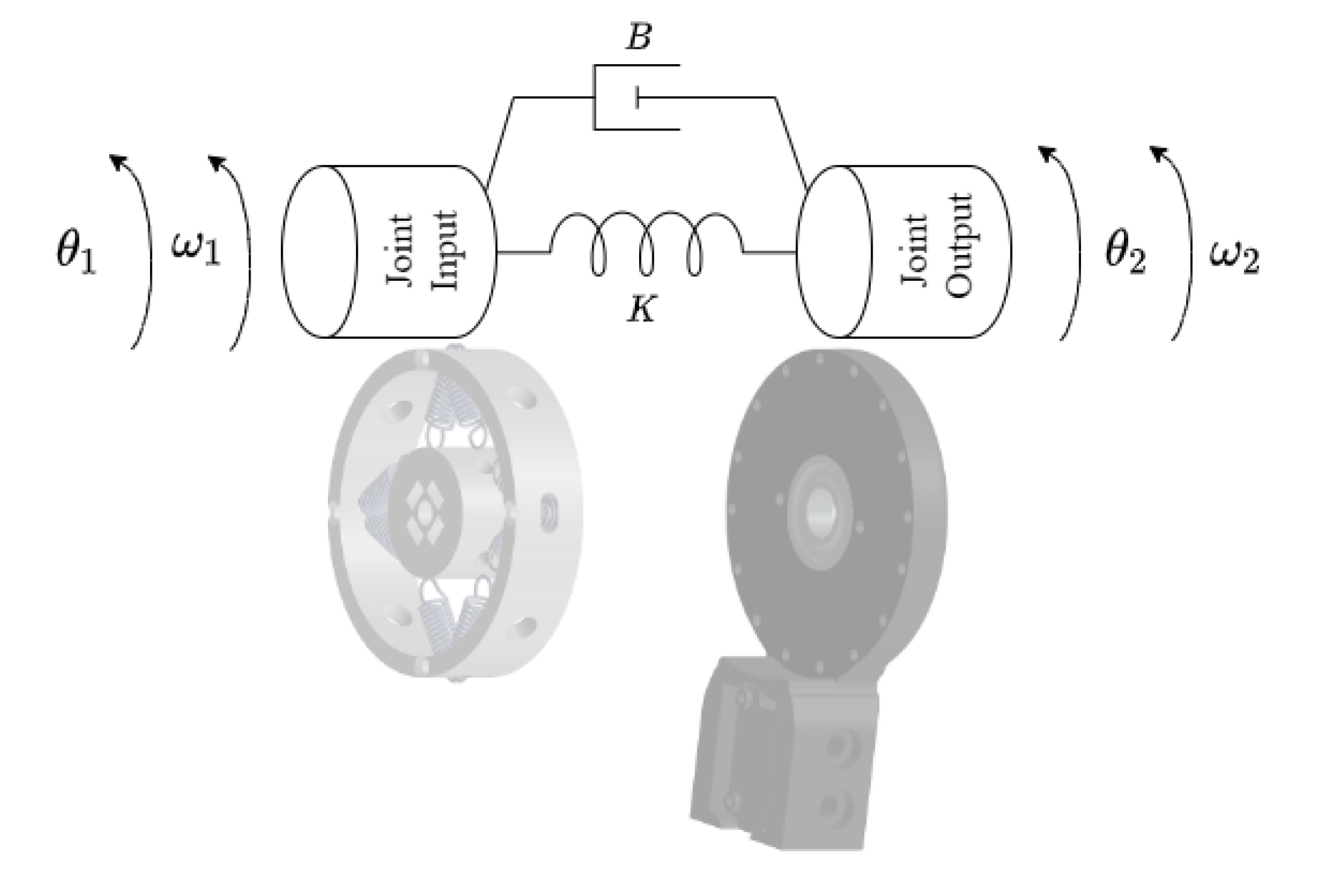
The conceptual representation of this system is illustrated in Figure 3. The linear differential equations that represent it are presented below.

The spring induced torque can be modeled by spring constant (K) multiplied by the difference between the input and output angular positions.

$${\tau }_K=K·({\theta }_2-{\theta }_1)$$

(1)

The viscous induced torque can be represented as the damping coefficient (B) multiplied by the difference between the input and output angular speeds.

$${\tau }_B=B·\left(\frac{d{\theta }_2\left(t\right)}{dt}-\frac{d{\theta }_1\left(t\right)}{dt}\right)$$

(2)

Now, since during our experiments the input position is fixed, ${\theta }_1$ and ${\omega }_1$ are equal to zero. So, the system angular acceleration over time can be obtained through

$$\frac{d{\omega }_2\left(t\right)}{dt}=\frac{1}{J}(-K{\theta }_2-B{\omega }_2)$$

(3)

Using only the derivatives of ${\theta }_2$, the previous equation becomes

$$J·\frac{d^2{\theta }_2\left(t\right)}{dt}+B·\frac{d{\theta }_2\left(t\right)}{dt}+K·{\theta }_2\left(t\right)=0$$

(4)

As can be seen from [22], the model presented is correct and can be applied to the modeling of a non-rigid joint. However, taking into account the non-linearity of the dead zone of the joint, it was decided to modify the presented model to predict this non-linearity by first changing Equation (3):

$$\frac{d\omega \left(t\right)}{dt}=\frac{1}{J}(-d\left(\theta \left(t\right)\right)-B\left(\omega \left(t\right)\right))$$

(5)

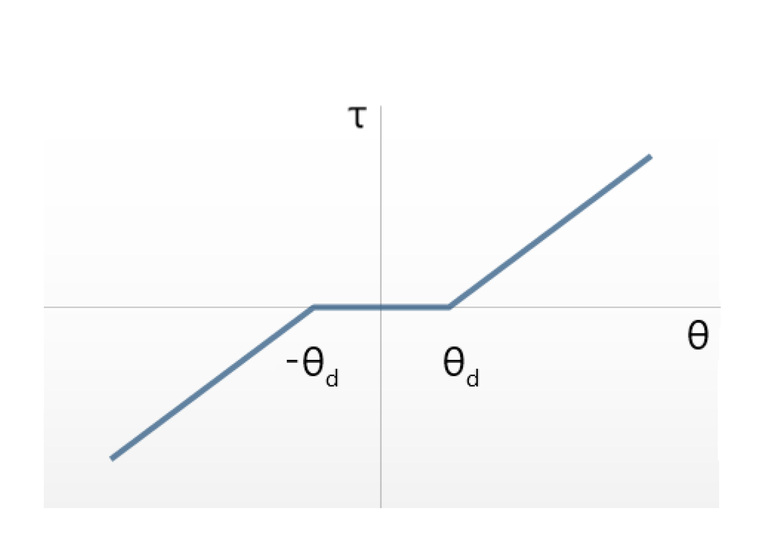
where $d\left(\theta \right)$ is introduced to model the dead-zone and $B\left(\omega \right)$ to model the viscous friction. $d\left(\theta \right)$ is defined by Equation (6), where $-{\theta }_d$ and ${\theta }_d$ are the dead zone left and right limits, as illustrated in Figure 4, while $B\left(\omega \right)$ is defined by Equation (7).

$$d\left(\theta \right)=\left\{\begin{array}{cc}(\theta -{\theta }_d)·K& \mathrm{if} \theta >{\theta }_d\\ 0& \mathrm{if}-{\theta }_d<\theta <{\theta }_d\\ (\theta +{\theta }_d)·K& \mathrm{if} \theta <-{\theta }_d\end{array}\right.$$

(6)

$$B\left(\omega \right)=\left\{\begin{array}{cc}B·\omega +G·(\omega -G_d)& \mathrm{if} \omega >G_d\\ B·\omega & \mathrm{if}-G_d<\omega <G_d\\ B·\omega +G·(\omega +G_d)& \mathrm{if} \omega <-G_d\end{array}\right.$$

(7)

Again, it is considered that the initial conditions cannot be null, so $\theta \left(0\right)={\theta }_0$ and angular speed are considered null, $\omega \left(0\right)=0$. Another important note is that, for the discretization, it was considered that $\theta [-2]=\theta [-1]=\theta \left[0\right]$. Thus,

$$\omega \left(t\right)=\frac{d\theta \left(t\right)}{dt}\simeq \frac{\Delta \theta }{\Delta t}$$

(8)

$$\omega \left[k\right]=\frac{\Delta \theta }{\Delta t}=\frac{\theta \left[k\right]-\theta [k-1]}{\Delta t}$$

(9)

A finite difference approximation method was used to represent the referred model, more specifically a second-order central, presented in Equation (10) and manipulated to obtain the model presented in Equation (12).

$$\frac{d\omega \left(t\right)}{dt}=\frac{d^2\theta \left(t\right)}{d{t}^2}\simeq \frac{\theta [k+1]-2\theta \left[k\right]+\theta [k-1]}{\Delta t^2}$$

(10)

$$\frac{\theta [k+1]-2\theta \left[k\right]+\theta [k-1]}{\Delta t^2}=\frac{1}{J}\left(-d\left(\theta \right[k\left]\right)-B\left(\omega \right[k\left]\right)\right)$$

(11)

$$\theta [k+1]=\frac{\Delta t^2}{J}\left(-d\left(\theta \right[k\left]\right)-B\left(\omega \right[k\left]\right)\right)+2\theta \left[k\right]-\theta [k-1]$$

(12)

Although the model is not used in this article, given that it is relatively easy to develop a physical prototype to tune and test both the system and controllers, it can be included in a realistic software simulation. It is expected that the next step of this work will include several of the developed joints, and therefore this simulation will be developed in the future.

2.3. Control Strategy

As mentioned in Section 1, it makes sense that a non-rigid joint increases the ability of the robotic system to operate in unstructured environments, and also increases its tolerance to impacts, i.e., impacts with a small force on objects or people, and finally enables detection of a breaking point and movement in the direction of this applied force.

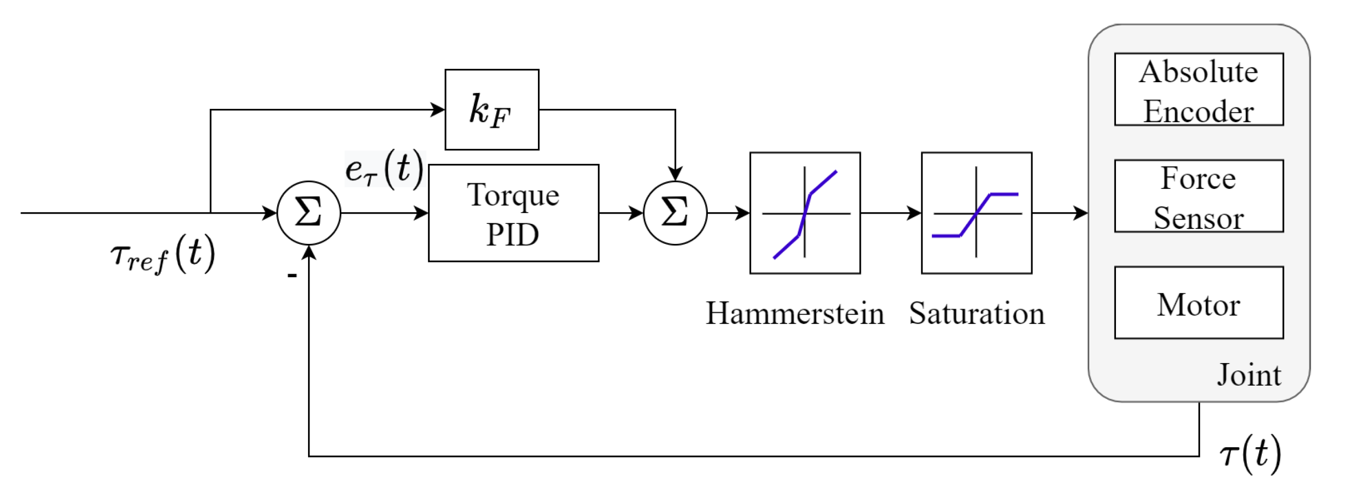
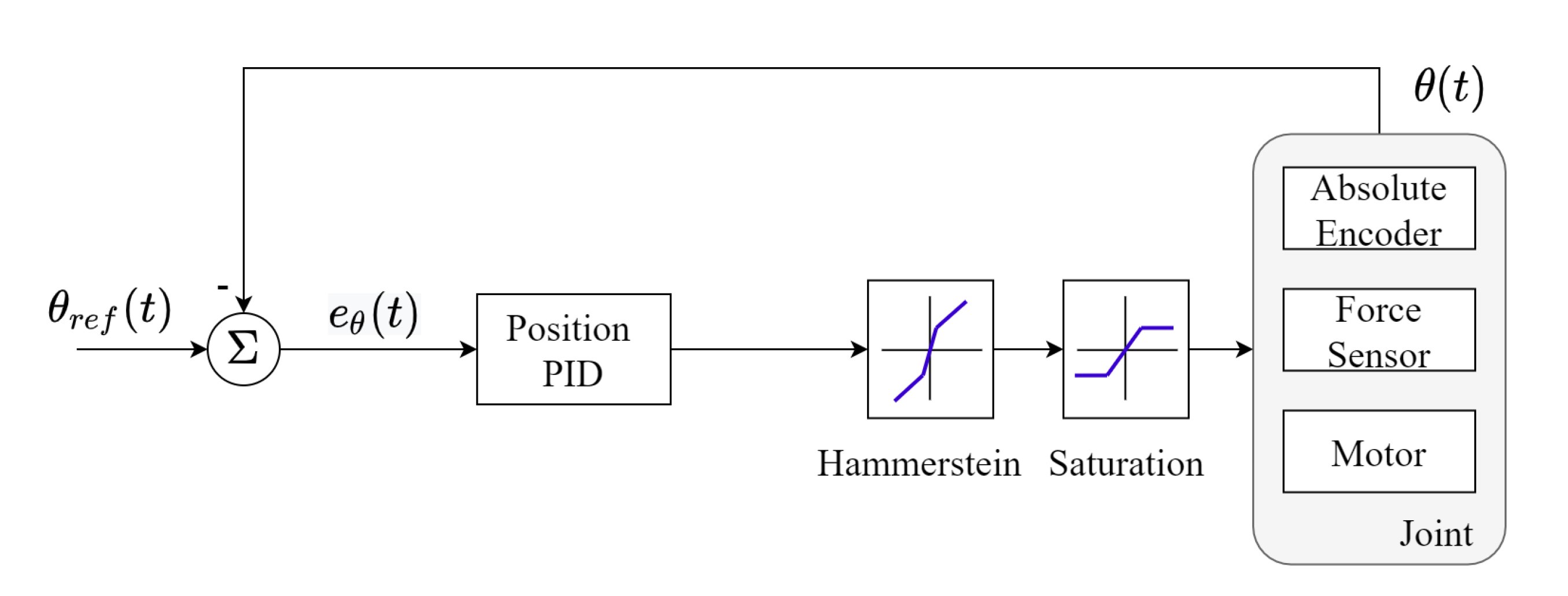
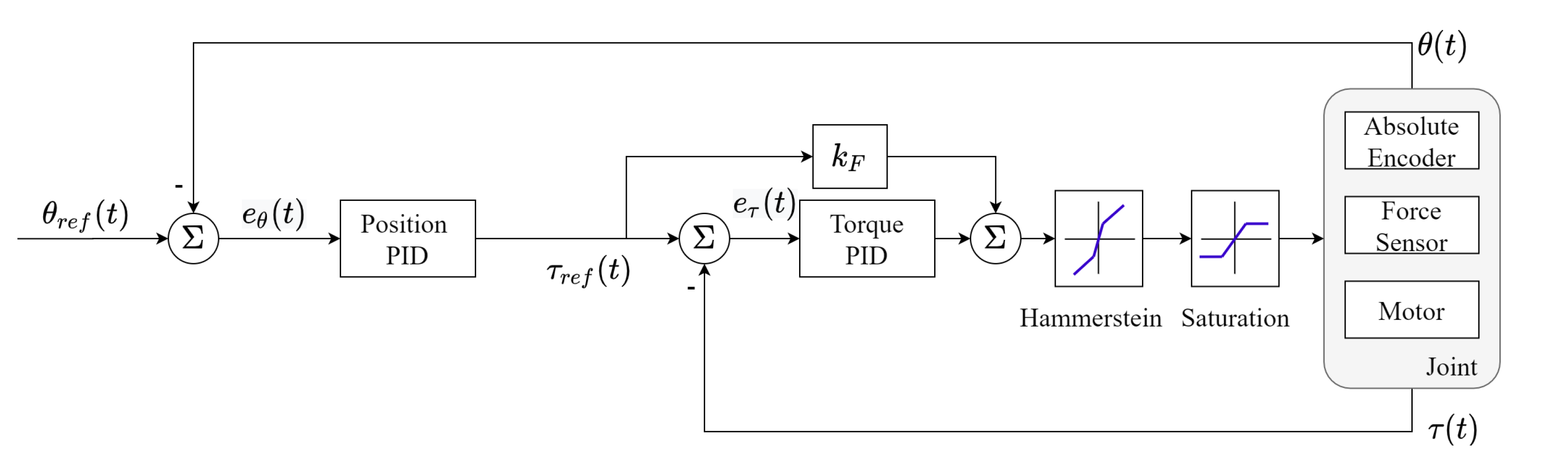
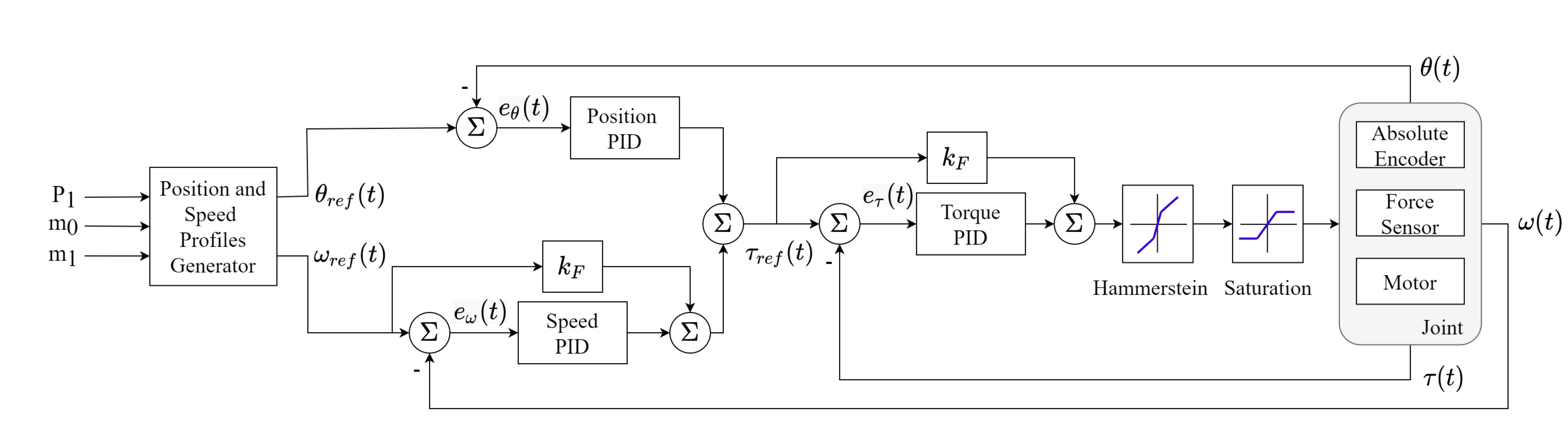
Although several types of strategies can be used to control the joint, the strategy chosen for the mode of operation that was intended for this platform was the compliant control. The main controllers are the position controller and the speed controller, as both have PI controllers, with a feedforward block added to the speed. Then the force controller is used in cascade with the two previous ones, the result of them being the force controller setpoint, using only a P controller with feedforward, since the introduction of the smallest integral component has destabilized the system. A Hammerstein block is used after the controller and before the motor to reduce the dead zone of the link. Finally, a saturation block is applied to define the limits of the admissible force. This method corresponds to the premise of compliant control.

It should be noted that this strategy is also an evolution of the one previously used in [22], as it adds a level of complexity that becomes necessary to respond to non-predicted external disturbances.

Taking into account the system used, which is similar to the solution proposed in [22], it was decided to use smoothed profiles for the speed and position of the motor controller. This is an improvement compared to the previous approach. The current approach allows the controller to be recalculated if the user decides to change the point or the final slope of the trajectory. For this purpose, the Hermite cubic polynomial was used to obtain the trajectory functions, taking into account that it fulfills the requirement that only the reference, the initial and final slope need to be specified in order to obtain a smoothed function from there. This function is very useful when the end point and/or the slope in the middle of the trajectory are changed, for which it is only necessary to supply the trajectory generator with the new end references and obtain them from the data that already have the initial values. Some considerations that have been made are mentioned below.

$$\begin{array}{c}P\left(0\right)=P_0\\ P\left(1\right)=P_1\\ m\left(0\right)=m_0=P^{\prime }\left(0\right)\\ m\left(1\right)=m_1=P^{\prime }\left(1\right)\\ t\in [0,1]\end{array}$$

Considering the latter, the polynomial takes the following form:

$$P\left(t\right)=\underset{h_{00}\left(t\right)}{\underbrace{(2t^3-3t^2+1)}}{P}_0+\underset{h_{10}\left(t\right)}{\underbrace{(t^3-2t^2+t)}}{m}_0+\underset{h_{01}\left(t\right)}{\underbrace{(-2t^3+3t^2)}}{P}_1+\underset{h_{11}\left(t\right)}{\underbrace{(t^3-t^2)}}{m}_1$$

(13)

The $h_{xx}$ functions can be represented as

$$\begin{array}{cc}\hfill h_{00}\left(t\right)& =(2t^3-3t^2+1)\hfill \\ \hfill h_{10}\left(t\right)& =(t^3-2t^2+t)\hfill \\ \hfill h_{01}\left(t\right)& =(-2t^3+3t^2)\hfill \\ \hfill h_{11}\left(t\right)& =(t^3-t^2)\hfill \end{array}$$

(14)

and their derivatives represented as

$$\begin{array}{cc}\hfill \frac{d{h}_{00}\left(t\right)}{dt}& =(6t^2-6t)\hfill \\ \hfill \frac{d{h}_{10}\left(t\right)}{dt}& =(3t^2-4t+1)\hfill \\ \hfill \frac{d{h}_{01}\left(t\right)}{dt}& =(-6t^2+6t)\hfill \\ \hfill \frac{d{h}_{11}\left(t\right)}{dt}& =(3t^2-2t)\hfill \end{array}$$

(15)

Now, considering that $t\in [0,\Delta ]$, the equations for $\theta \left(t\right)$ and $\omega \left(t\right)$ become

$$\theta \left(t\right)=P\left(t\right)=(2t^3-3t^2+1)P_0+(t^3-2t^2+t)m_0\Delta +(-2t^3+3t^2)P_1+(t^3-t^2)m_1\Delta$$

(16)

$$\omega \left(t\right)=\frac{dP\left(t\right)}{dt}=(6t^2-6t)P_0+(3t^2-4t+1)m_0\Delta +(-6t^2+6t)P_1+(3t^2-2t)m_1\Delta$$

(17)

where $P_0,P_1,m_0\mathrm{and}{m}_1$ are the initial and final points and slopes of the spline, respectively.

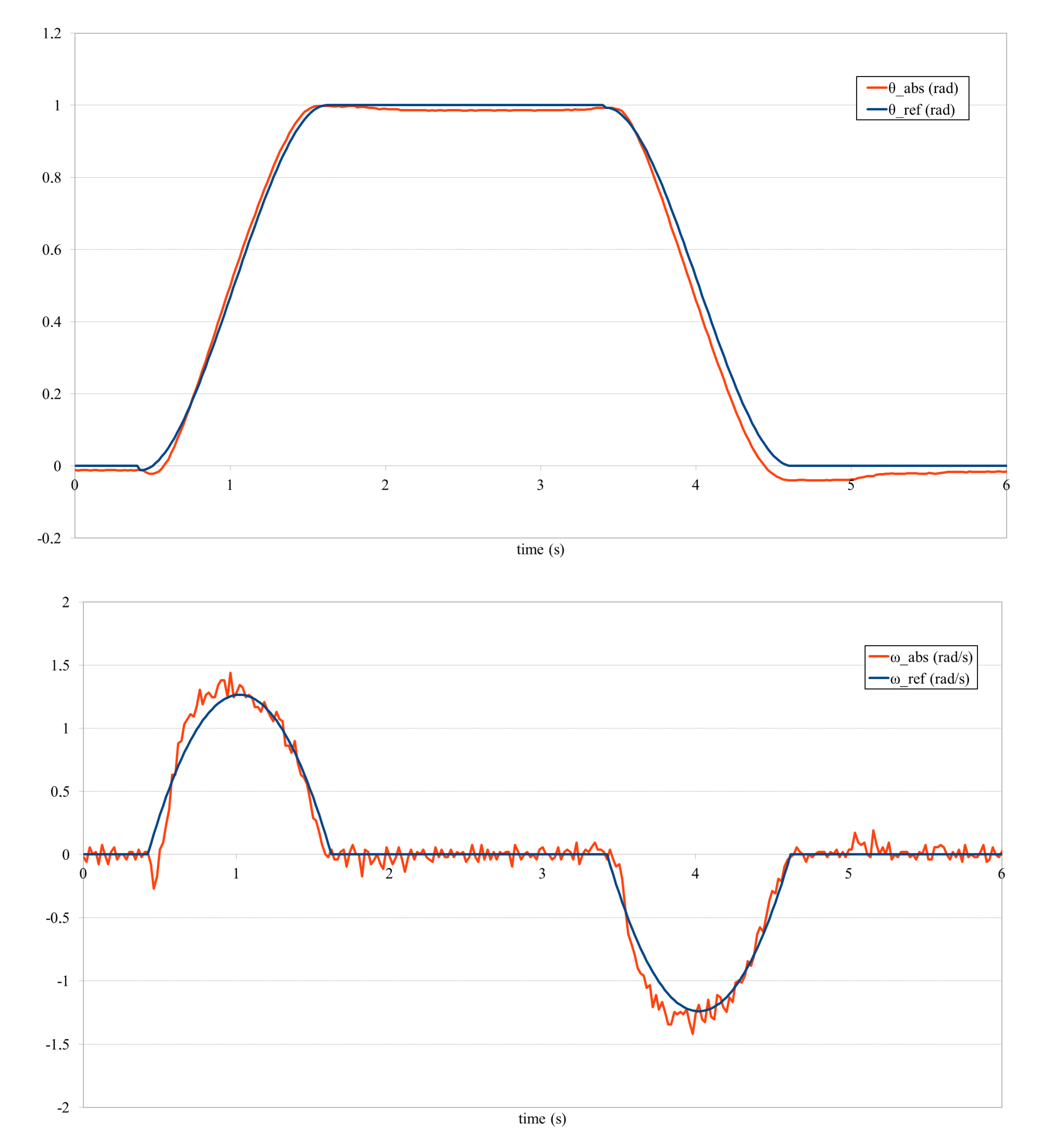
The position and velocity profiles are graphically illustrated as the reference signal further on in Section 4.2.5.

3. Experimental Setup

3.1. Platform

The model presented in the previous subsection has some variables that can only be obtained by estimation methods. In this case, it has been defined that the estimation process is offline, taking into account that the physical properties of the joint are not expected to change during operation. Taking this into account, the sensor and detection system used to obtain the necessary data for the estimation is presented.

The required data are the force applied to the joint connected to the joint and the respective angle. To obtain all the necessary data, it is necessary to use a load cell (TAL220) with the corresponding amplifier (HX711), as well as an absolute encoder (AS5048) and a development board (Arduino Uno).

For the further development of this work, the use of the CQGB37Y001 DC motor was chosen to control the joint. In contrast to the previous work [22] a motor without a worm gearbox was used, one with an inline gearbox being used instead. This was due to the high friction that the worm gear brought to the system, which resulted in a significant increase in the dead zone of the motor. The motor was powered by an external 12 V power supply and a Motor Driver Shield (Arduino Motor Shield v2). It is important to mention that the data concerning the encoder was also collected on the Arduino for control purposes.

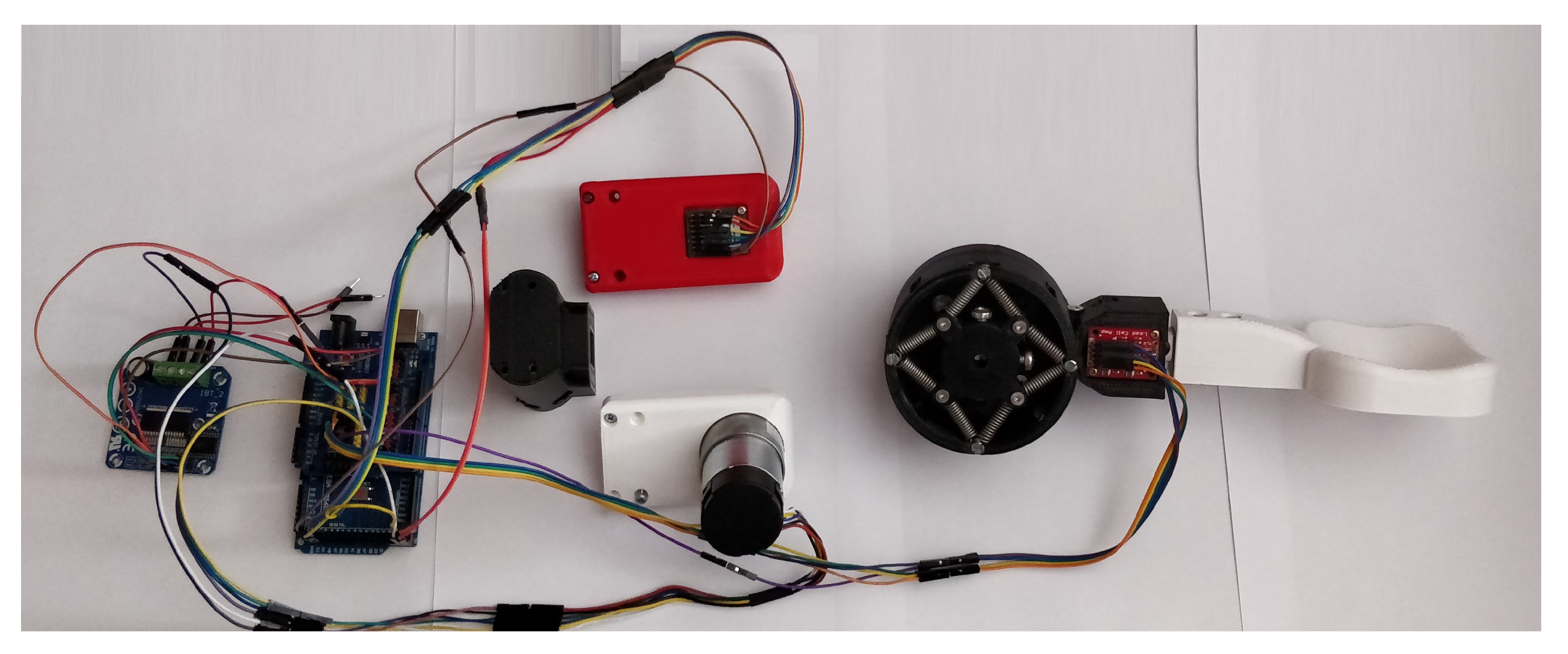
A platform was designed both for the modeling process and for the controller development process presented later, which made it possible to obtain all necessary data and to test the controller. It has a spoon-shaped part attached to the outer part of the load cell to facilitate the placement of weights of known mass and the application of external forces. This platform is shown in Figure 5 and Figure 6.

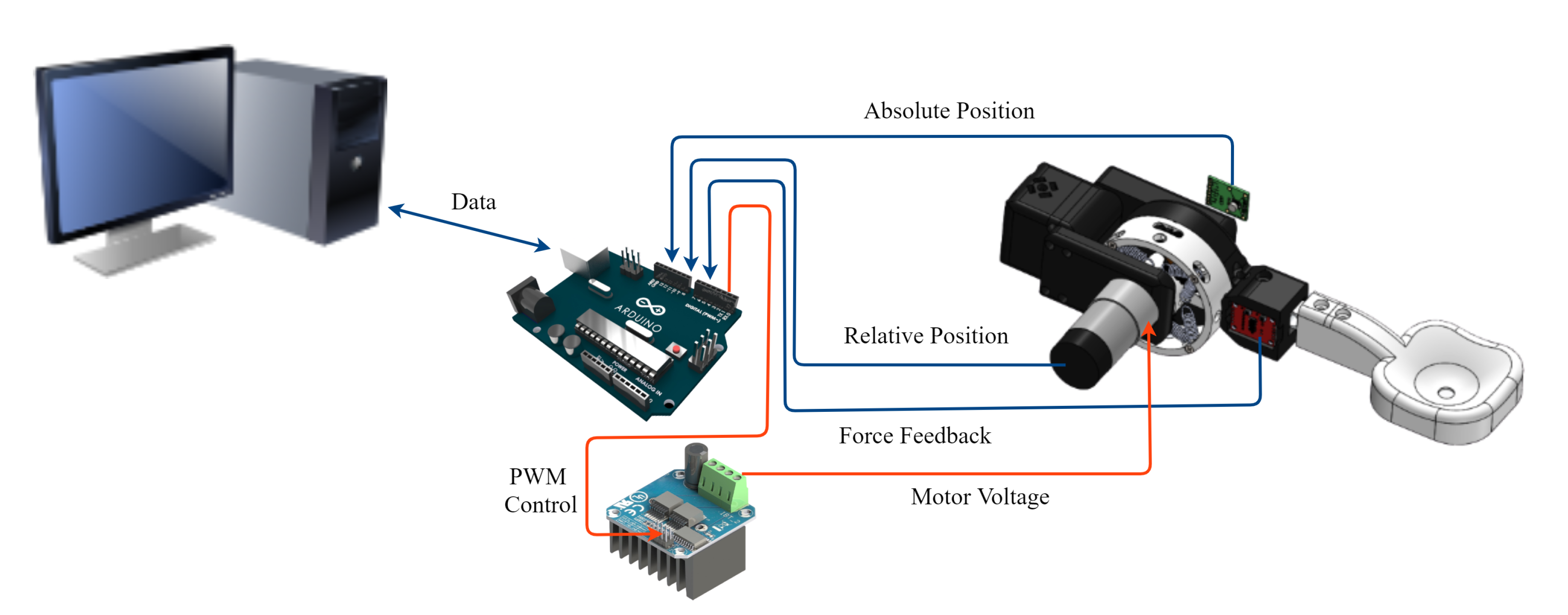
The complete system associated with the data acquisition is represented in Figure 6.

In addition to the hardware setup, it was also necessary to develop software capable of collecting data to realistically define the model and act as a driver for the development of the controllers for the joint. So it was defined to use two programs, one in Arduino and another in a PC.

The software running on the PC is responsible for communicating with the Arduino software, i.e., it has the ability to change parameters in real time, such as sensor offsets, controller tuning parameters and others. It also displays the important variables graphically or numerically.

The Arduino software is responsible for data processing, decision making, controller definitions, knowledge of acceleration profiles, velocity and position and for controlling the motor with the desired voltage. It sends the important data to the PC software, which collects and stores the data for later graphical analysis, with the main cycle running at 50 Hz.

3.2. Test Description

It is necessary to estimate the moment of inertia, the spring constant and the damping coefficient included in the joint’s model. Two tests are performed to estimate these parameters and to define the model:

• A force is applied manually to the link pulling it to either side of the joint, thereby increasing the maximum angle of rotation. For each of these angles, the applied force is sensed, which is then converted into a torque, in parallel to the respective angle;
• Again, the link is pulled to both sides of the joint, but this time the link is released and is expected to stabilize until it reaches the angle of rest. Similar to the previous test, the applied force and its respective angle are recorded.

To test the controllers, some movements were performed:

• Angular positioning control;
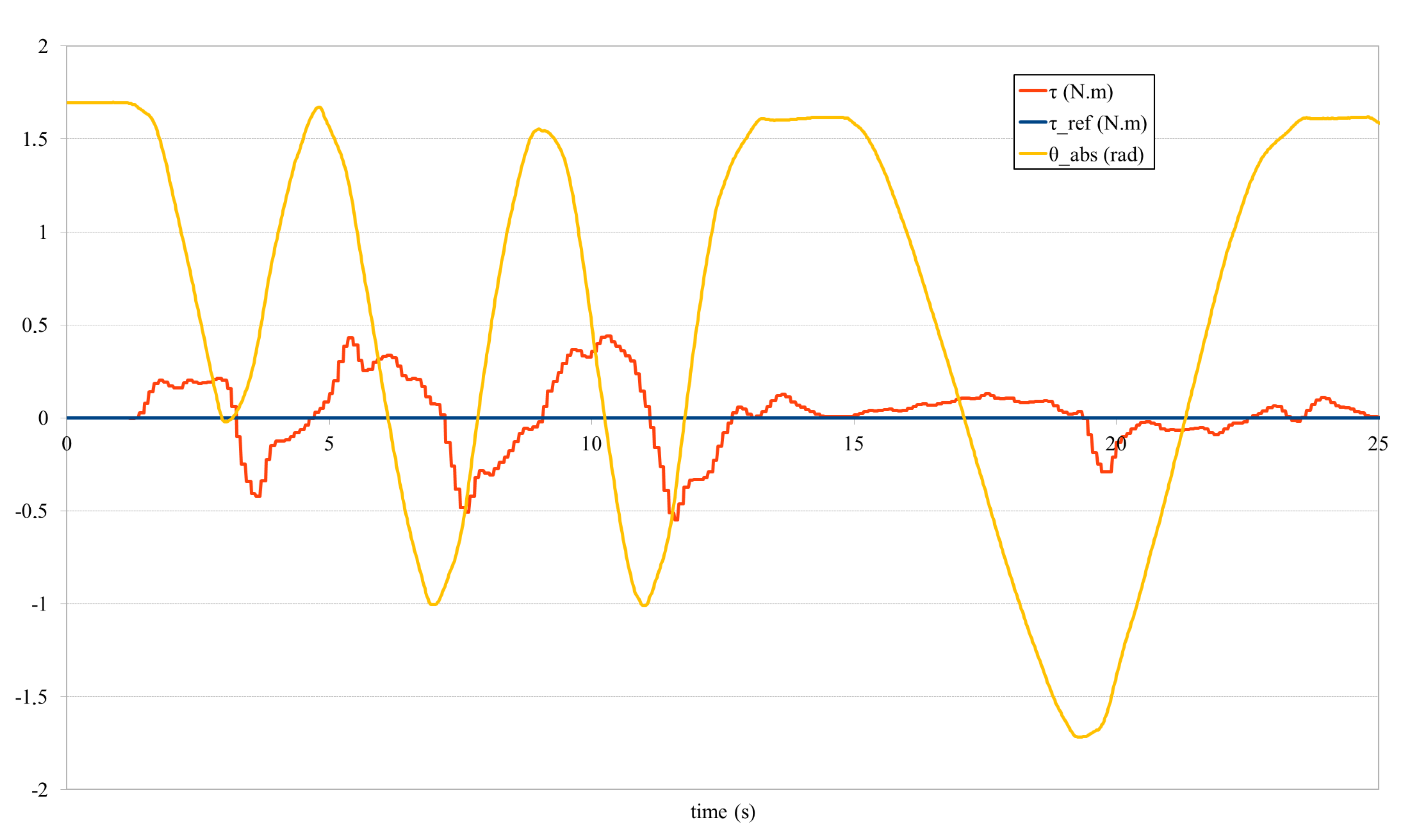
• Backdrivability—force controller, with 0 reference;
• Compliant position controller without obstacle in the trajectory;
• Compliant position controller with obstacle in the trajectory;
• Trajectory following for a desired position, without obstacle;
• Weight placement without reaching the defined force limit;
• Weight placement exceeding the defined force limit;

4. Results

In this paper a number of experiments are described, which were used to define the model and test the designed controllers. As mentioned above, the data are collected every 20 milliseconds and stored for further analysis.

4.1. Model

Through the experiments it was determined that the dead zone of the joint must be included in the model, as mentioned in Equation (6). The slopes of the negative and positive parts of the diagram were associated with Equation (1), and the spring constant could be obtained by calculating the mean value of the slopes. The value obtained for K was 16.92 N/m.

After obtaining the value for K, the values for the moment of inertia and damping coefficient could then be determined using the approximation function shown in Equation (12). The collected data are graphically captured and introduced in Figure 7 in blue in the form of an angle versus time, while the optimization result of the model is shown in orange. After the optimization process had been completed, the following data were entered for J and B values of 0.007 Kg · m${}^2$ and 1.218 N · s /m were obtained. Figure 8 graphically shows the absolute error of the model compared to the real position and the numerical error values are summarized in

Table 2. Absolute error analysis.

Absolute Error
Maximum	0.0197 rad
Average	0.0026 rad

.

The estimated parameters are shown in

Table 3. Estimated joint parameters.

Parameters
K	16.92 N/m
B	1.218 N·s/m
J	0.007 Kg·${\mathrm{m}}^2$

.

Initially, data were collected based on the behavior of the joint without control in the presence of an external, manually introduced disturbance of known strength to evaluate its response, which is shown in the right graphic in Figure 9. The angular movement that occurred was due to the contraction and expansion of the springs and rotary damper. In addition, the response of the current joint can be compared to that of the previous version [22], which is presented in the left graphic of Figure 9. As one can see, the new joint has a smaller vibration amplitude (it decreases from about 0.2 to about 0.06 rad), but also its settling time is drastically lower (it decreases from about 2 to about 0.4 s). Based on these data, it can be concluded that the new joint can be introduced into a system and that it will be more stable compared to the previous one. These values are summarized in

Table 4. Comparison between joints.

	Joint v1	Joint v7
Maximum Amplitude	0.2 rad	0.06 rad
Settling Time	2 s	0.4 s

.

4.2. Control

4.2.1. Angular Positioning Control

For lower-level control, position and force controllers were tested independently of each other. Figure 10 presents the first controller block diagram, for pure position control. Figure 11 presents the response to a step in the reference of the position.

4.2.2. Backdrivability—Force Controller, with 0 Reference

For the pure force controller, Figure 12 shows the controller block diagram. Figure 13 presents the obtained data for the experiment.

An important aspect of this controller is that it allows implementation of a backdrivability function to the joint, as shown in Figure 13. The force limit was defined as 0 N·m, and therefore the control followed the movement of the operator after registering an absolute maximum error of 0.5 N·m in rapid movements and 0.27 N·m in slower ones. As can be observed, the movement was performed between about 1.7 and −1.7 radian with several variations over about 24 s. Although this function is currently not useful for the work under development, it can be very interesting for use in a robot manipulator.

4.2.3. Compliant Position Controller without Obstacle in the Trajectory

After the low-level controllers were individually tuned, the cascade controller was developed with a combination of position, speed and force control. The controller block diagram is presented in Figure 14.

The next test was to establish a reference in position and a limit for the force controller. The diagram in Figure 15 represents a movement up to an angle of 1 radian and back to 0 with no obstacles in the way.

4.2.4. Compliant Position Controller with Obstacle in the Trajectory

Figure 16 shows the data relating to a positioning attempt with an obstacle, where the allowable absolute force limit has been defined as 0.7 N·m. As can be seen, the reference is not reached, but the force limit has been reached and the position remains in the closer possible position.

4.2.5. Trajectory Following a Desired Position, without Obstacle in the Way

When the trajectory generator mentioned in the previous section was introduced into the control system (as can be seen in Figure 17), the compliant control system with force limitation and trajectory tracking was implemented and tested. The diagram in Figure 18 shows a movement to an angle of 1 radian (up), without obstacles, and the corresponding speed behavior (down).

4.2.6. Weight Placement without Reaching the Strength Limit

Finally, a test for the placement of unknown disturbances was carried out by introducing loads into the spoon-shaped part. First, a load was placed that did not exceed the defined force limit, so that it was able to hold the load in the defined position (0 rad). The data associated with this test are presented in Figure 19.

4.2.7. Weight Placement Exceeding the Strength Limit

In the second iteration of the test, two loads were placed, with placement of the second one exceeding the limit, causing the joint to give way and drop the loads. Figure 20 represents the behavior of the joint during this situation.

5. Conclusions and Future Work

First of all, it is worth mentioning that the maximum developed force of the presented joint has been significantly increased, which has allowed several problems to be solved that occurred in the previous solution, as well as some that were found during the development of the present version. There was also a significant improvement, which is a possible approach towards its use in an industrial environment.

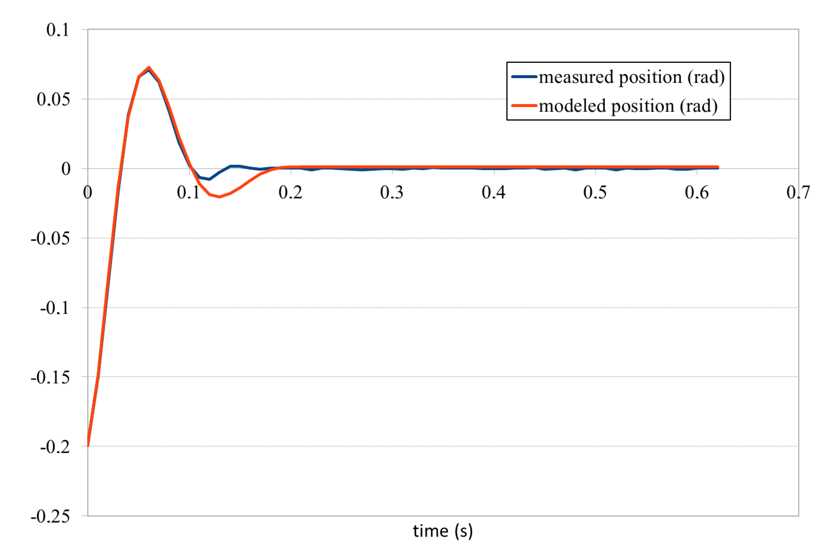
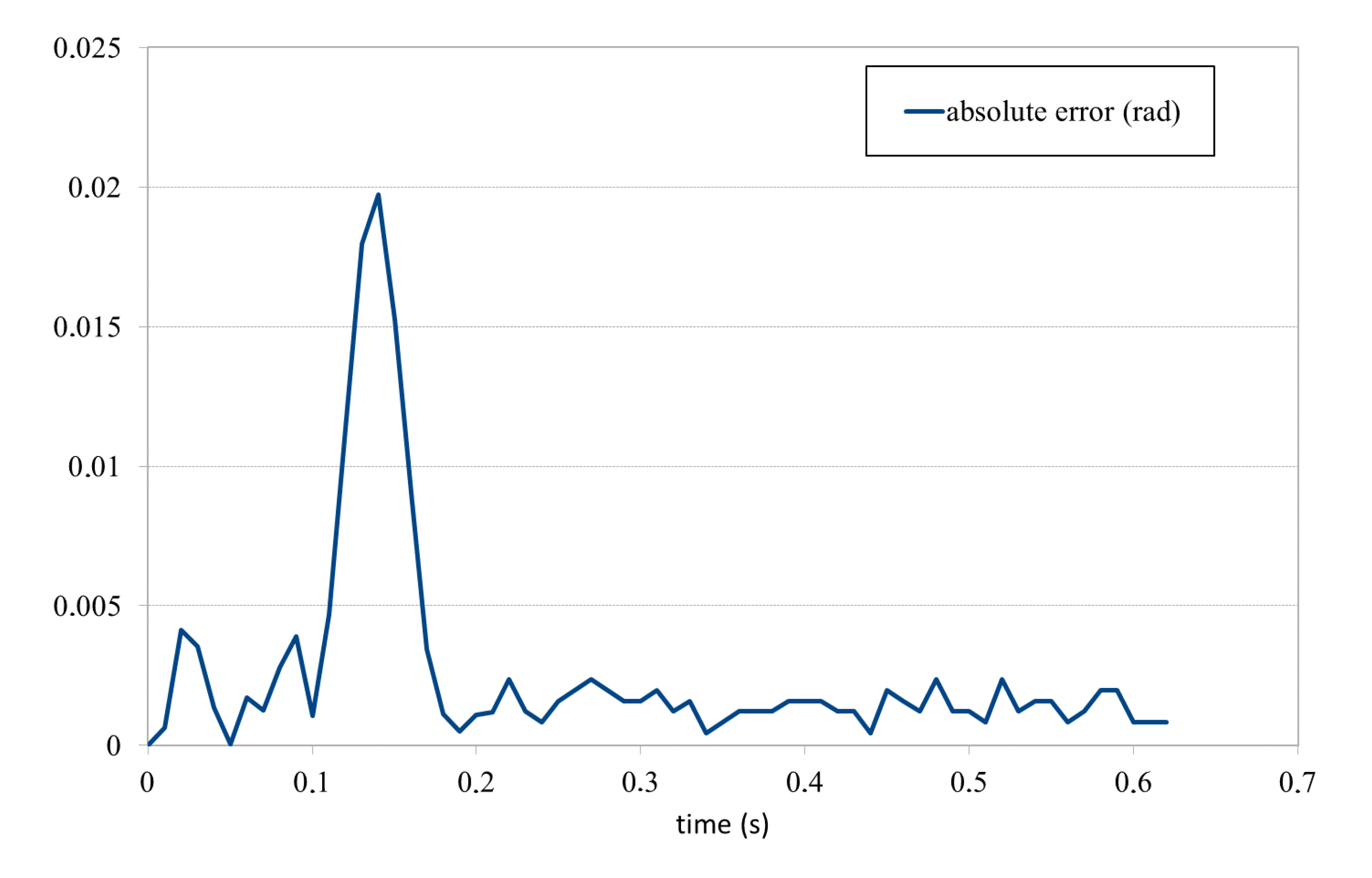
Apart from the design component, the entire modeling component can also be evaluated as positive, so that in the future it will be possible to replicate this system in a simulator and achieve very realistic results. The parameter estimation resulted in a spring constant of 16.92 N/m, a damping coefficient of 1.218 N · s/m and a moment of inertia of 0.007 Kg· m${}^2$. The model has an absolute maximum error of 0.0197 rad, while the average absolute error is 0.0026 rad.

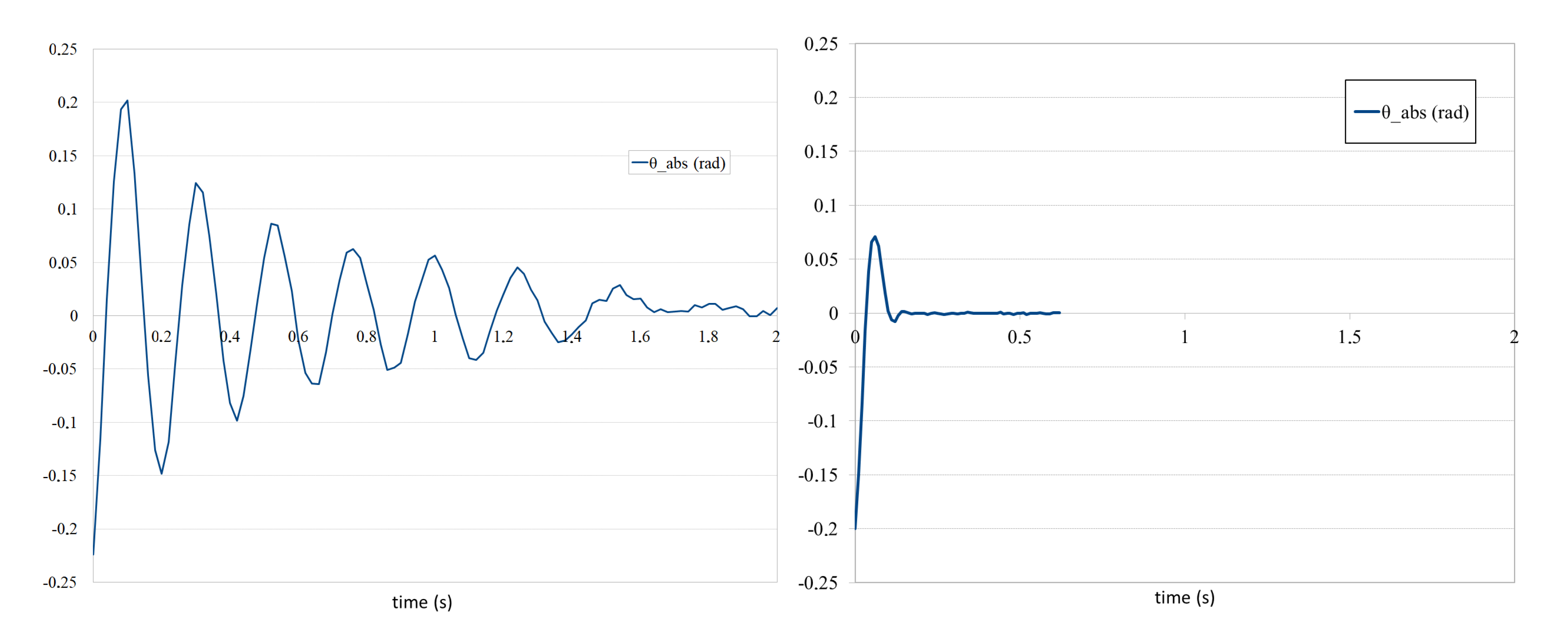
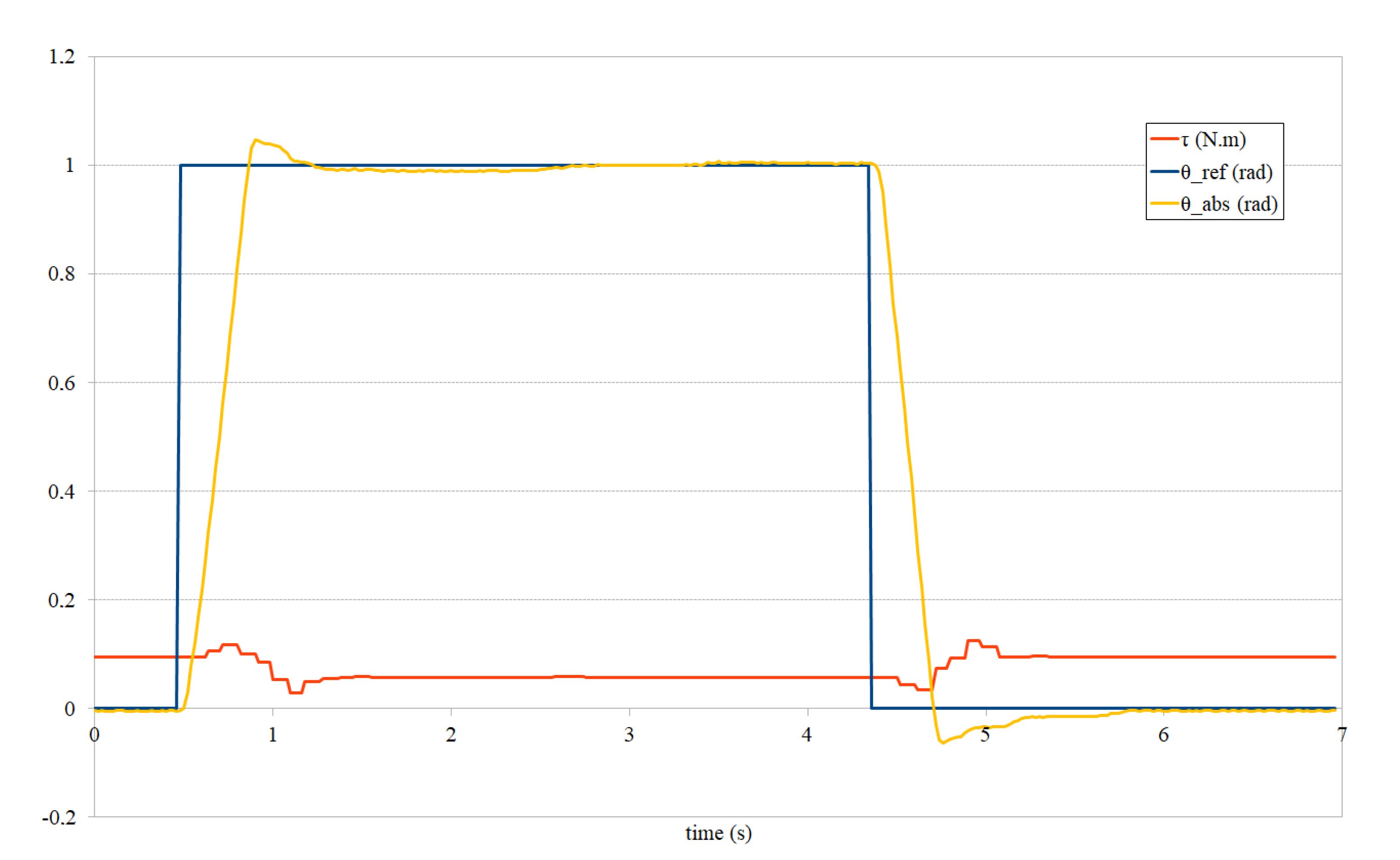
Compared to the previous joint and to those mentioned in the introduction, this version has introduced a significant damping component that reduces the high-frequency vibrations caused by the springs, and the system remains purely passive. As can be seen from Figure 9, the joint’s maximum amplitude decreases from approximately 0.2 to 0.06 rad. Also, its settling time decreases from around 2 to 0.4 s.

At the control level, it was found that the additional compliant component with the force sensor is an important improvement that allows the system and environment to be safer and more responsive to external disturbances.

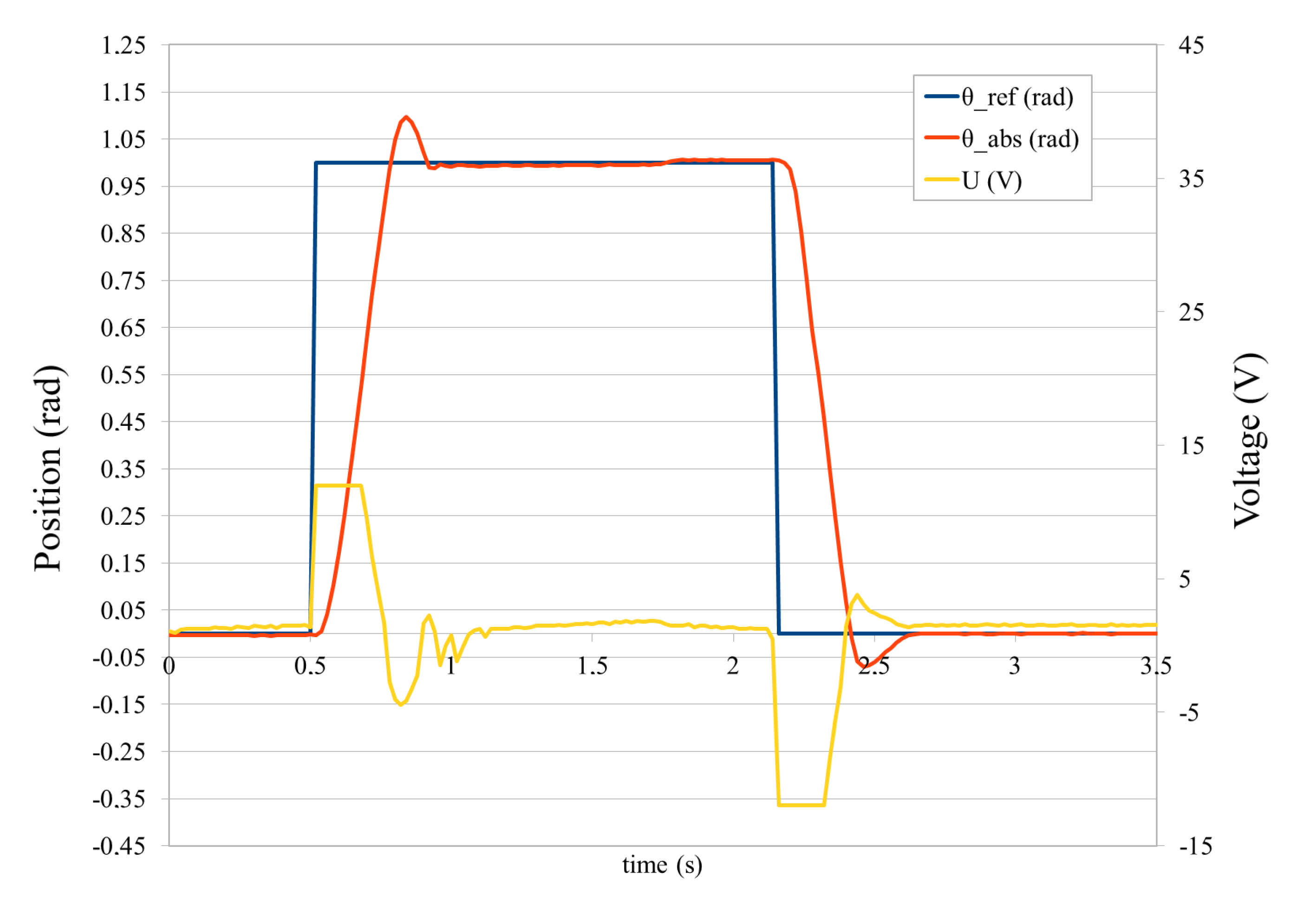
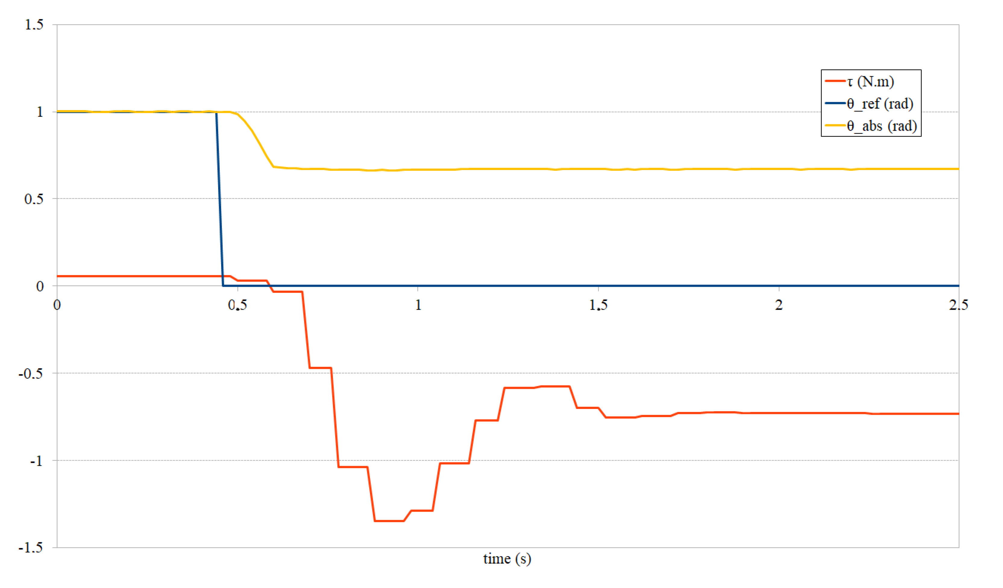
The force-limiting component is also very important with regard to hitting obstacles, and by setting a limit value that is not harmful to the system or the environment, operational safety is always guaranteed. The backdrivability example shows that, while moving at a relatively high speed, on a trajectory with a movement of 2.5 rad, the maximum absolute error was around 0.5 N · m.

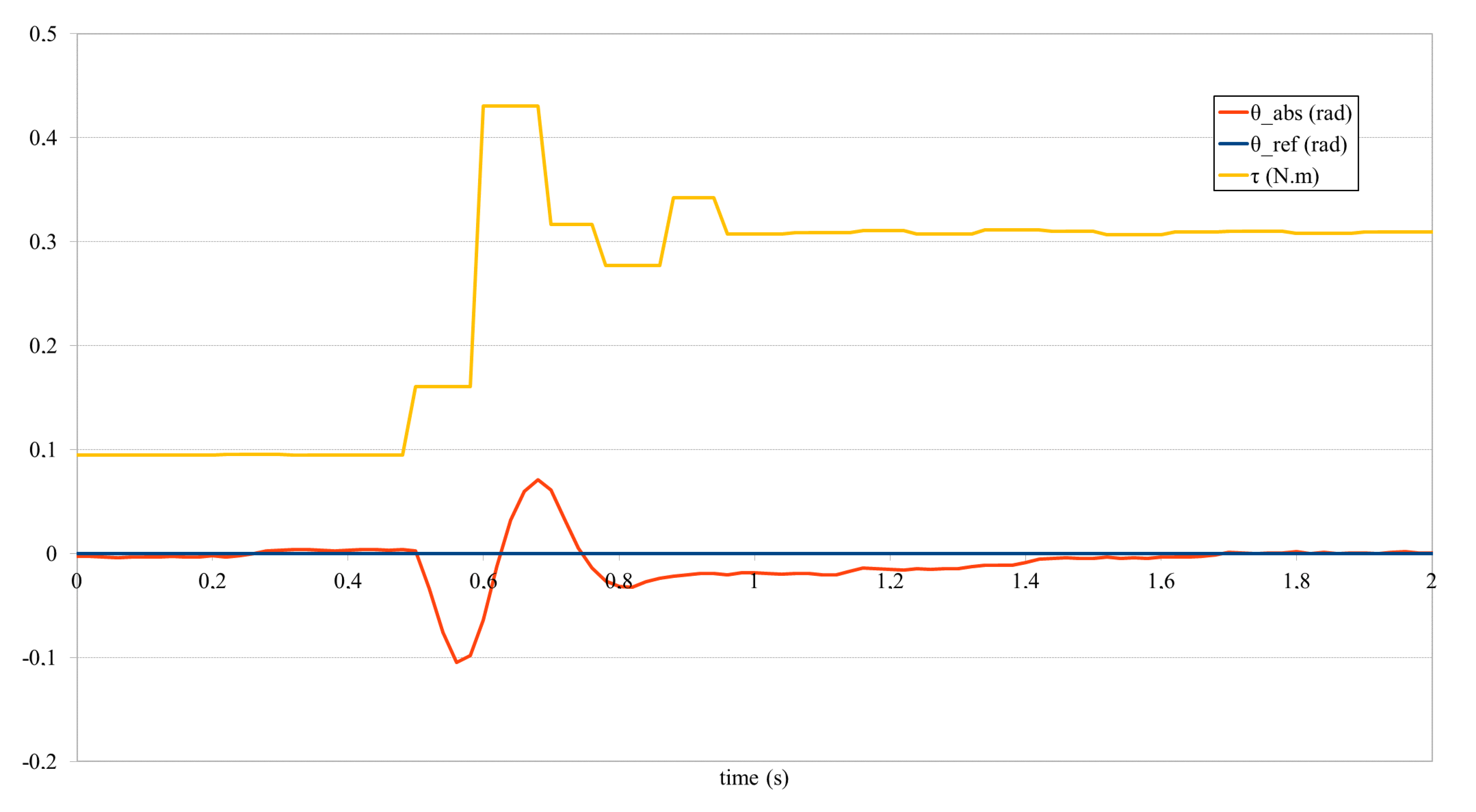
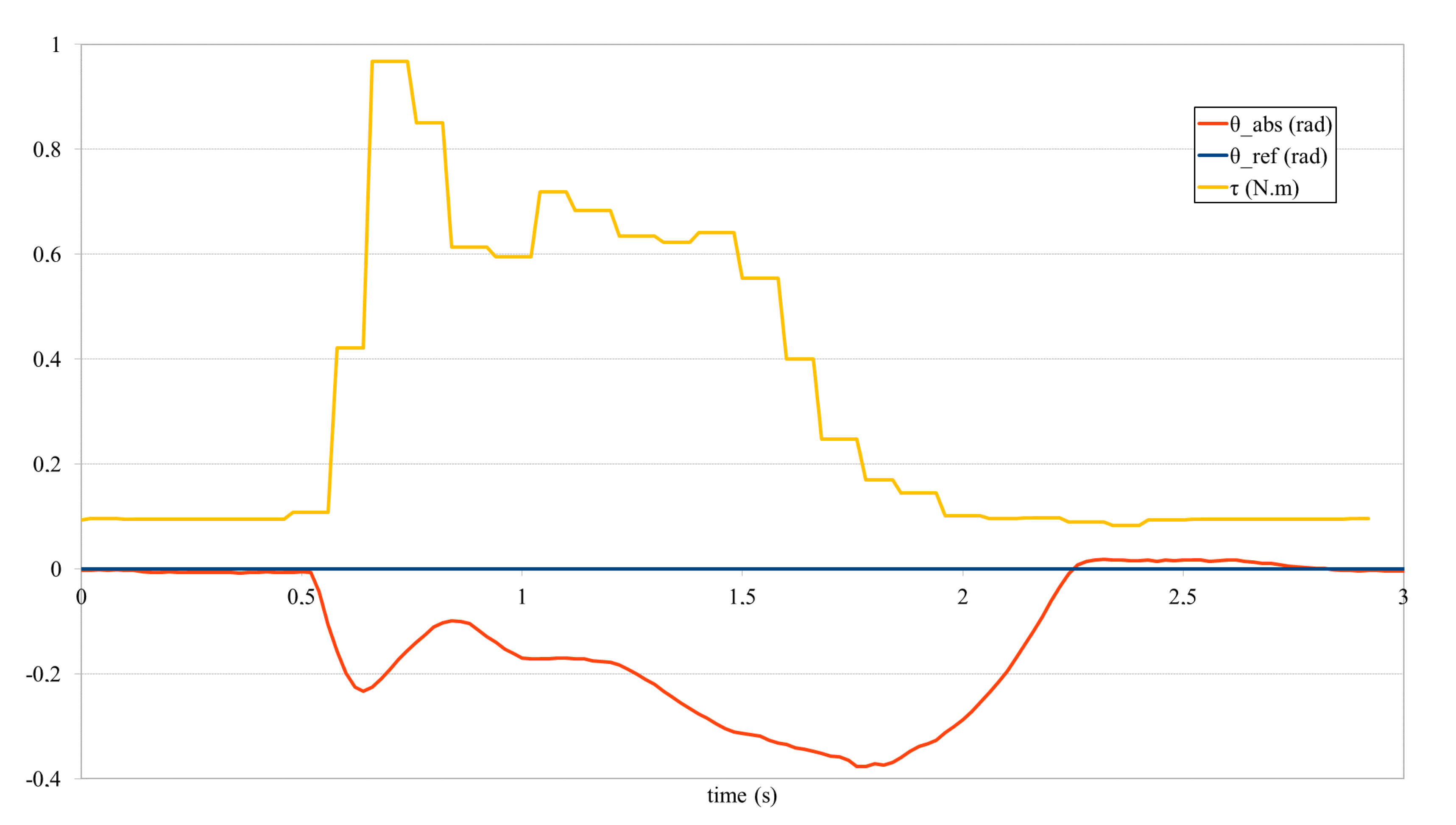
In addition, the compliant control disturbance rejection with a position reference had a very positive response, without reaching the strength limit, and stabilized the system in around 0.4 s. For the force limit exceeded test, it also demonstrated its speed in response when this limit is reached, giving up and letting the joint go in around 0.4 s.

Taking all the above points into account, it can be concluded that the developed solution achieves the desired results.

With regard to future work, the authors intend to apply this joint and the developed control system in robot manipulators or robot links aimed at autonomous robot vehicles.

Considering that the joint can be used for several purposes and that an accurate model is already built, it may be appropriate to use realistic simulation tools that allow testing without the need for physical design, which would speed up the exploration and tuning of controllers in a more systematic approach. Since it is expected that the number of joints working simultaneously will increase, this would be a major advantage.

At this moment, the authors’ focus is to develop systems based on passive springs and dampers. For future work, it is intended to improve the system by using semi-active dampers.