A Performance Study of the Impact of Different Perturbation Methods on the Efficiency of GVNS for Solving TSP


Abstract
:1. Introduction
- Cyclic neighborhood change step: Whether there is an improvement in some neighborhood or not, the search continues in the next neighborhood structure in the list.
- Pipe neighborhood change step: If the current solution is improved in some neighborhood, exploration in that neighborhood will continue.
- Skewed neighborhood change step: Accept as new incumbent alternatives that not only improve solutions, but also some that are worse than the current incumbent solution. Such a neighborhood change step is intended to allow valley exploration away from the incumbent solution. A trial solution is evaluated taking into consideration not only the trial’s objective values and the incumbent solution, but also their distance.
Organization
2. GVNS Heuristics
2.1. Neighborhood Structures
- 1-0 Relocate. This move removes node i from its current position in the route and re-inserts it after a selected node b.
- 2-Opt. The 2-Opt move breaks two arcs in the current solution and reconnects them in a different way.
- 1-1 Exchange. This move swaps two nodes in the current route.
| Algorithm 1 pipe-VND. |
|
2.2. Shaking Methods
- Evolutionary, biological-inspired algorithms.
- Swarm intelligence algorithms inspired by swarm/agent group behavior.
- Social and cultural algorithms inspired by society’s interactions and beliefs.
- Inspired by quantum physics, Quantum-inspired algorithms.
| Algorithm 2 Shake_1. |
|
Quantum Computing Principles
| Algorithm 3 Shake_2. |
|
| Algorithm 4 Shake_3. |
|
2.3. GVNS Schemes
| Algorithm 5 GVNS_1. |
|
| Algorithm 6 GVNS_2. |
|
| Algorithm 7 GVNS_3. |
|
3. Computational Analysis
3.1. Computing Environment & Parameter Settings
3.2. Computational Results
4. Statistical Analysis on Computational Results
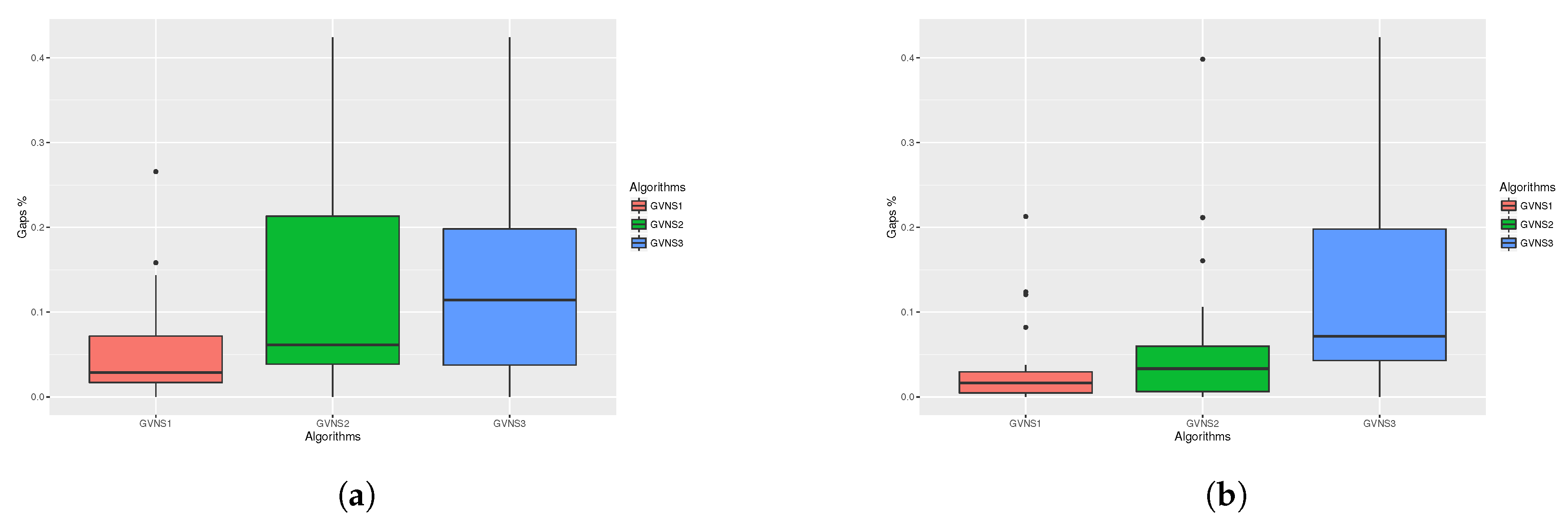
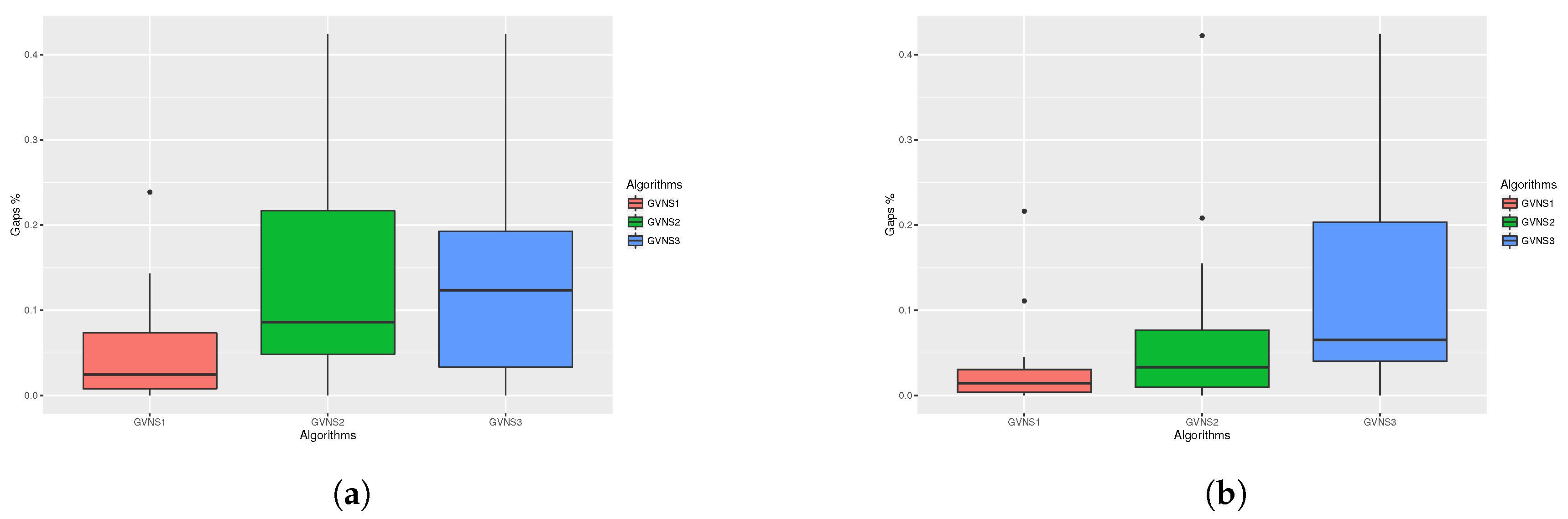
4.1. Statistical Analysis on aTSP Results
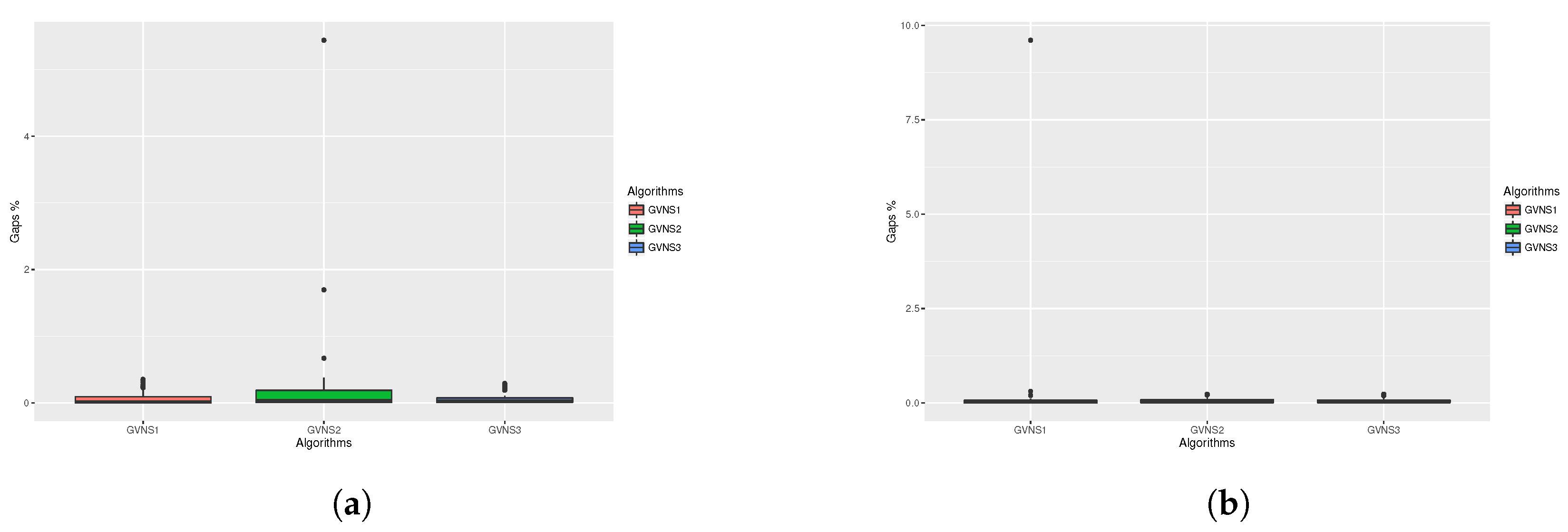
4.2. Statistical Analysis on sTSP
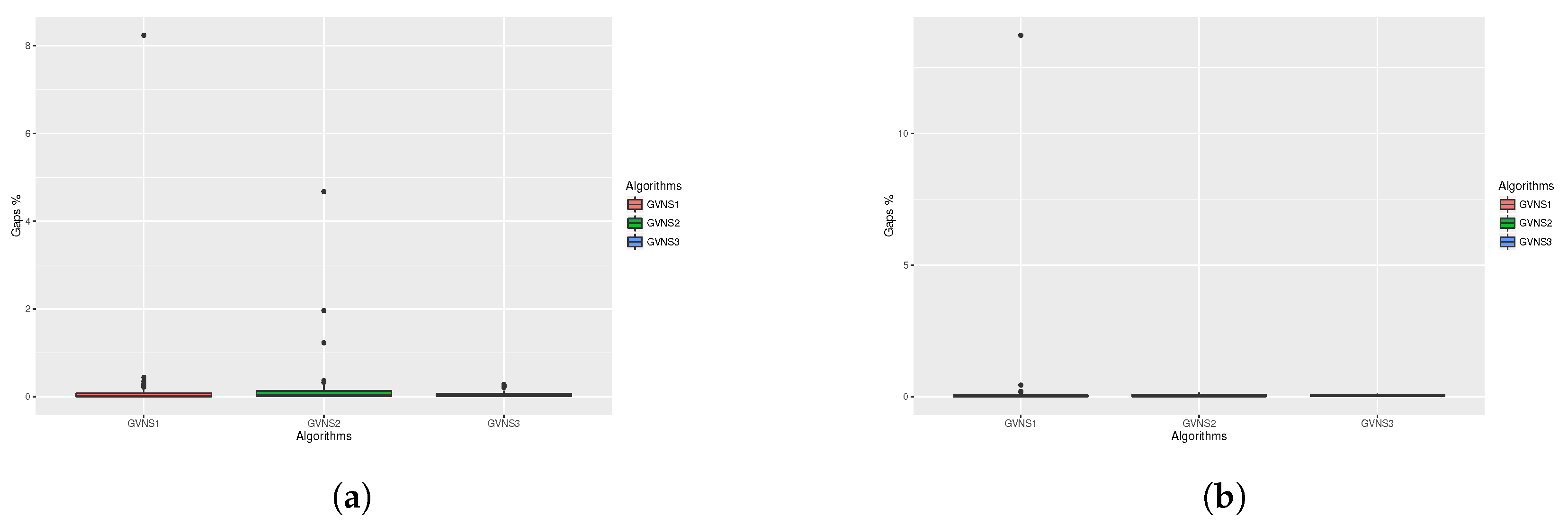
4.3. Statistical Analysis on nTSP
5. Comparison with Recent Similar Works
6. Conclusions and Future Work
Author Contributions
Funding
Conflicts of Interest
Abbreviations
| TSP | Traveling Salesman Problem |
| VNS | Variable Neighborhood Search |
| GVNS | General Variable Neighborhood Search |
| GA | Genetic Algorithm |
| SA | Simulated Annealing |
| TS | Tabu Search |
| ACO | Ant Colony Optimization |
| TPO | Tree Physiology Optimization |
References
- Mladenovic, N.; Hansen, P. Variable neighborhood search. Comput. Oper. Res. 1997, 24, 1097–1100. [Google Scholar] [CrossRef]
- Hansen, P.; Mladenovic, N.; Todosijevic, R.; Hanafi, S. Variable neighborhood search: Basics and variants. EURO J. Comput. Optim. 2017, 5, 423–454. [Google Scholar] [CrossRef]
- Mladenovic, N.; Todosijevic, R.; Uroševic, D. Less is more: Basic variable neighborhood search for minimum differential dispersion problem. Inf. Sci. 2016, 326, 160–171. [Google Scholar] [CrossRef]
- Mladenović, N.; Sifaleras, A.; Sörensen, K. Editorial to the Special Cluster on Variable Neighborhood Search, Variants and Recent Applications. Int. Trans. Oper. Res. 2017, 24, 507–508. [Google Scholar] [CrossRef]
- Karakostas, P.; Sifaleras, A.; Georgiadis, C. Basic VNS algorithms for solving the pollution location inventory routing problem. In Proceedings of the LNCS Proc. of the 6th International Conference on Variable Neighborhood Search (ICVNS 2018), Sithonia, Greece, 4–7 October 2018; Sifaleras, A., Salhi, S., Brimberg, J., Eds.; Springer: Berlin, Germany, 2019; Volume 11328. [Google Scholar]
- Karakostas, P.; Sifaleras, A.; Georgiadis, C. A general variable neighborhood search-based solution approach for the location-inventory-routing problem with distribution outsourcing. Comput. Chem. Eng. 2019, 126, 263–279. [Google Scholar] [CrossRef]
- Papalitsas, C.; Karakostas, P.; Andronikos, T.; Sioutas, S.; Giannakis, K. Combinatorial GVNS (General Variable Neighborhood Search) Optimization for Dynamic Garbage Collection. Algorithms 2018, 11, 38. [Google Scholar] [CrossRef]
- Sifaleras, A.; Konstantaras, I. General variable neighborhood search for the multi-product dynamic lot sizing problem in closed-loop supply chain. Electron. Notes Discret. Math. 2015, 47, 69–76. [Google Scholar] [CrossRef]
- Sifaleras, A.; Konstantaras, I. Variable neighborhood descent heuristic for solving reverse logistics multi-item dynamic lot-sizing problems. Comput. Oper. Res. 2017, 78, 385–392. [Google Scholar] [CrossRef]
- Silva, M.A.; Souza, S.R.; Souza, M.J.; Filho, M.F.F. Hybrid metaheuristics and multi-agent systems for solving optimization problems A review of frameworks and a comparative analysis. Appl. Soft Comput. 2018, 71, 433–459. [Google Scholar] [CrossRef]
- Duan, Q.; Liao, T.; Yi, H. A comparative study of different local search application strategies in hybrid metaheuristics. Appl. Soft Comput. 2013, 13, 1464–1477. [Google Scholar] [CrossRef]
- Huber, S.; Geiger, M.J. Order matters–A Variable Neighborhood Search for the Swap-Body Vehicle Routing Problem. Eur. J. Oper. Res. 2017, 263, 419–445. [Google Scholar] [CrossRef]
- Papalitsas, C.; Giannakis, K.; Andronikos, T.; Theotokis, D.; Sifaleras, A. Initialization methods for the TSP with Time Windows using Variable Neighborhood Search. In Proceedings of the IEEE Proc. of the 6th International Conference on Information, Intelligence, Systems and Applications (IISA 2015), Corfu, Greece, 6–8 July 2015. [Google Scholar]
- Papalitsas, C.; Karakostas, P.; Andronikos, T. Studying the impact of perturbation methods on the efficiency of GVNS for the ATSP. In LNCS Proc. of the 6th International Conference on Variable Neighborhood Search (ICVNS 2018), Sithonia, Greece, 4–7 October 2018; Sifaleras, A., Salhi, S., Brimberg, J., Eds.; Springer: Berlin, Germany, 2019; Volume 11328. [Google Scholar]
- Papalitsas, C.; Karakostas, P.; Kastampolidou, K. A Quantum Inspired GVNS: Some Preliminary Results; Vlamos, P., Ed.; GeNeDis 2016; Springer International Publishing: Cham, Switzerland, 2017; pp. 281–289. [Google Scholar]
- Nunes, D.C.L. Fundamentals of Natural Computing: Basic Concepts, Algorithms, and Applications; Chapman & Hall/CRC: Boca Raton, FL, USA, 2006. [Google Scholar]
- Dey, S.; Bhattacharyya, S.; Maulik, U. New quantum inspired meta-heuristic techniques for multi-level colour image thresholding. Appl. Soft Comput. 2016, 46, 677–702. [Google Scholar] [CrossRef]
- Feynman, R.P. Simulating physics with computers. Int. J. Theor. Phys. 1982, 21, 467–488. [Google Scholar] [CrossRef]
- Feynman, R.P.; Hey, J.; Allen, R.W. Feynman Lectures on Computation; Longman Publishing Co., Inc.: Cambridge, MA, USA, 1998. [Google Scholar]
- Coffin, M.; Saltzman, M.J. Statistical Analysis of Computational Tests of Algorithms and Heuristics. INFORMS J. Comput. 2000, 12, 24–44. [Google Scholar] [CrossRef]
- Halim, A.H.; Ismail, I. Combinatorial optimization: Comparison of heuristic algorithms in travelling salesman problem. Arch. Comput. Methods Eng. 2019, 26, 367–380. [Google Scholar] [CrossRef]
- Hore, S.; Chatterjee, A.; Dewanji, A. Improving variable neighborhood search to solve the traveling salesman problem. Appl. Soft Comput. 2018, 68, 83–91. [Google Scholar] [CrossRef]


| Instance | zOpt | GVNS_1 | GVNS_2 | GVNS_3 | GAP_1 (%) | GAP_2 (%) | GAP_3 (%) |
|---|---|---|---|---|---|---|---|
| br17.atsp | 39 | 39 | 39 | 39 | 0.00 | 0.00 | 0.00 |
| ft53.atsp | 6905 | 7189 | 7328 | 7737 | 4.11 | 6.13 | 12.05 |
| ft70.atsp | 38673 | 39782 | 40691 | 40537 | 2.87 | 5.22 | 4.82 |
| ftv33.atsp | 1286 | 1318 | 1339 | 1450 | 2.49 | 4.12 | 12.75 |
| ftv35.atsp | 1473 | 1484 | 1499 | 1596 | 0.75 | 1.77 | 8.35 |
| ftv38.atsp | 1530 | 1546 | 1585 | 1579 | 1.05 | 3.59 | 3.20 |
| ftv44.atsp | 1613 | 1651 | 1760 | 1797 | 2.36 | 9.11 | 11.41 |
| ftv47.atsp | 1778 | 1821 | 1992 | 2101 | 2.42 | 12.04 | 18.17 |
| ftv55.atsp | 1608 | 1666 | 1985 | 1912 | 3.61 | 23.45 | 18.91 |
| ftv64.atsp | 1839 | 1961 | 2382 | 2395 | 6.63 | 29.53 | 30.23 |
| ftv70.atsp | 1950 | 2136 | 2557 | 2484 | 9.54 | 31.13 | 27.38 |
| ftv170.atsp | 2755 | 3487 | 3923 | 3923 | 26.57 | 42.40 | 42.40 |
| kro124p.atsp | 36230 | 39024 | 43187 | 40259 | 7.71 | 19.20 | 11.12 |
| p43.atsp | 5620 | 5620 | 5623 | 5658 | 0.00 | 0.05 | 0.68 |
| rbg323.atsp | 1326 | 1516 | 1563 | 1626 | 14.32 | 17.87 | 22.62 |
| rbg358.atsp | 1163 | 1347 | 1437 | 1404 | 15.82 | 23.55 | 20.72 |
| rbg403.atsp | 2465 | 2535 | 2587 | 2565 | 9.78 | 4.42 | 11.76 |
| rbg443.atsp | 2720 | 2814 | 2859 | 2814 | 3.46 | 5.11 | 3.46 |
| ry48p.atsp | 14422 | 14549 | 14901 | 14738 | 0.88 | 3.32 | 2.19 |
| Average | 6599.74 | 6920.26 | 7328.37 | 7190.21 | 12.33 | 12.64 | 24.10 |
| Instance | zOpt | GVNS_1 | GVNS_2 | GVNS_3 | GAP_1 (%) | GAP_2 (%) | GAP_3 (%) |
|---|---|---|---|---|---|---|---|
| br17.atsp | 39 | 39 | 39 | 39 | 0.00 | 0.00 | 0.00 |
| ft53.atsp | 6905 | 7043 | 7135 | 7674 | 2.00 | 3.33 | 11.14 |
| ft70.atsp | 38673 | 39507 | 40206 | 40539 | 2.16 | 3.96 | 4.83 |
| ftv33.atsp | 1286 | 1289 | 1286 | 1379 | 0.23 | 0.00 | 7.23 |
| ftv35.atsp | 1473 | 1476 | 1473 | 1533 | 0.20 | 0.00 | 4.07 |
| ftv38.atsp | 1530 | 1538 | 1541 | 1599 | 0.52 | 0.72 | 4.51 |
| ftv44.atsp | 1613 | 1632 | 1644 | 1728 | 1.18 | 1.92 | 7.13 |
| ftv47.atsp | 1778 | 1792 | 1816 | 1940 | 0.79 | 2.14 | 9.11 |
| ftv55.atsp | 1608 | 1642 | 1665 | 2012 | 2.11 | 3.54 | 25.12 |
| ftv64.atsp | 1839 | 1908 | 1986 | 2193 | 3.75 | 7.99 | 19.25 |
| ftv70.atsp | 1950 | 2110 | 2157 | 2346 | 8.21 | 10.62 | 20.31 |
| ftv170.atsp | 2755 | 3341 | 3852 | 3923 | 21.27 | 39.82 | 42.40 |
| kro124p.atsp | 36230 | 36501 | 37076 | 38195 | 0.75 | 2.34 | 5.42 |
| p43.atsp | 5620 | 5620 | 5620 | 5627 | 0.00 | 0.00 | 0.12 |
| rbg323.atsp | 1326 | 1486 | 1539 | 1633 | 12.06 | 16.06 | 23.15 |
| rbg358.atsp | 1163 | 1307 | 1409 | 1437 | 12.38 | 21.15 | 23.55 |
| rbg403.atsp | 2465 | 2510 | 2547 | 2554 | 11.76 | 11.76 | 11.76 |
| rbg443.atsp | 2720 | 2765 | 2824 | 2844 | 1.65 | 3.16 | 4.56 |
| ry48p.atsp | 14422 | 14480 | 14498 | 14659 | 0.40 | 0.12 | 1.64 |
| Average | 6599.74 | 6736.11 | 6858.58 | 7044.95 | 15.88 | 17.69 | 22.28 |
| Instance | zOpt | GVNS_1 | GVNS_2 | GVNS_3 | GAP_1 (%) | GAP_2 (%) | GAP_3 (%) |
|---|---|---|---|---|---|---|---|
| br17.atsp | 39 | 39 | 39 | 39 | 0.00 | 0.00 | 0.00 |
| ft53.atsp | 6905 | 7024 | 7498 | 7752 | 1.72 | 8.59 | 12.27 |
| ft70.atsp | 38673 | 39615 | 40827 | 40505 | 2.44 | 5.57 | 4.74 |
| ftv33.atsp | 1286 | 1330 | 1370 | 1454 | 3.42 | 6.53 | 13.06 |
| ftv35.atsp | 1473 | 1482 | 1519 | 1604 | 0.61 | 3.12 | 8.89 |
| ftv38.atsp | 1530 | 1547 | 1618 | 1576 | 1.11 | 5.75 | 3.01 |
| ftv44.atsp | 1613 | 1628 | 1839 | 1812 | 0.93 | 14.01 | 12.34 |
| ftv47.atsp | 1778 | 1787 | 2020 | 2097 | 0.51 | 13.61 | 17.94 |
| ftv55.atsp | 1608 | 1668 | 2012 | 1912 | 3.73 | 25.12 | 18.91 |
| ftv64.atsp | 1839 | 1951 | 2484 | 2476 | 6.09 | 35.07 | 34.64 |
| ftv70.atsp | 1950 | 2165 | 2571 | 2484 | 11.03 | 31.85 | 27.38 |
| ftv170.atsp | 2755 | 3412 | 3923 | 3923 | 23.85 | 42.40 | 42.40 |
| kro124p.atsp | 36230 | 39344 | 44243 | 40849 | 8.60 | 22.12 | 12.75 |
| p43.atsp | 5620 | 5620 | 5628 | 5657 | 0.00 | 0.14 | 0.66 |
| rbg323.atsp | 1326 | 1499 | 1576 | 1586 | 13.04 | 18.85 | 19.60 |
| rbg358.atsp | 1163 | 1329 | 1410 | 1406 | 14.27 | 21.23 | 20.89 |
| rbg403.atsp | 2465 | 2509 | 2586 | 2547 | 2.27 | 4.10 | 11.76 |
| rbg443.atsp | 2720 | 2808 | 2849 | 2811 | 3.24 | 4.74 | 3.35 |
| ry48p.atsp | 14422 | 14475 | 14936 | 14708 | 0.37 | 3.56 | 1.98 |
| Average | 6599.74 | 6906.95 | 7418.32 | 7220.95 | 5.29 | 13.96 | 24.78 |
| Instance | zOpt | GVNS_1 | GVNS_2 | GVNS_3 | GAP_1 (%) | GAP_2 (%) | GAP_3 (%) |
|---|---|---|---|---|---|---|---|
| br17.atsp | 39 | 39 | 39 | 39 | 0.00 | 0.00 | 0.00 |
| ft53.atsp | 6905 | 7043 | 7207 | 7773 | 2.00 | 4.37 | 12.57 |
| ft70.atsp | 38673 | 39358 | 40230 | 40588 | 1.77 | 4.03 | 4.95 |
| ftv33.atsp | 1286 | 1286 | 1290 | 1370 | 0.00 | 0.31 | 6.53 |
| ftv35.atsp | 1473 | 1474 | 1475 | 1509 | 0.07 | 0.14 | 2.44 |
| ftv38.atsp | 1530 | 1538 | 1555 | 1599 | 0.52 | 1.63 | 4.51 |
| ftv44.atsp | 1613 | 1636 | 1664 | 1731 | 1.43 | 3.16 | 7.32 |
| ftv47.atsp | 1778 | 1787 | 1837 | 1903 | 0.51 | 3.32 | 7.03 |
| ftv55.atsp | 1608 | 1640 | 1686 | 2012 | 1.99 | 4.85 | 25.12 |
| ftv64.atsp | 1839 | 1914 | 2032 | 2217 | 4.08 | 10.49 | 20.55 |
| ftv70.atsp | 1950 | 2038 | 2189 | 2342 | 4.51 | 12.26 | 20.10 |
| ftv170.atsp | 2755 | 3351 | 3918 | 3923 | 21.63 | 42.21 | 42.40 |
| kro124p.atsp | 36230 | 36379 | 37378 | 37915 | 0.41 | 3.17 | 4.65 |
| p43.atsp | 5620 | 5620 | 5620 | 5625 | 0.00 | 0.00 | 0.09 |
| rbg323.atsp | 1326 | 1473 | 1531 | 1610 | 11.08 | 15.46 | 21.41 |
| rbg358.atsp | 1163 | 1292 | 1405 | 1435 | 11.09 | 20.80 | 23.38 |
| rbg403.atsp | 2465 | 2498 | 2547 | 2553 | 1.30 | 3.25 | 11.76 |
| rbg443.atsp | 2720 | 2771 | 2822 | 2842 | 1.88 | 3.75 | 4.49 |
| ry48p.atsp | 14422 | 14468 | 14464 | 14678 | 0.32 | 0.29 | 1.78 |
| Average | 6599.74 | 6716.05 | 6888.89 | 7034.95 | 3.28 | 7.05 | 22.16 |
| Instance | zOpt | GVNS_1 | GVNS_2 | GVNS_3 | GAP_1 | GAP_2 | GAP_3 |
|---|---|---|---|---|---|---|---|
| a280.tsp | 2579 | 2683 | 2739 | 2745 | 4.03 | 6.20 | 6.44 |
| att48.tsp | 10628 | 10628 | 10628 | 10635 | 0.00 | 0.00 | 0.07 |
| bayg29.tsp | 1610 | 1610 | 1610 | 1610 | 0.00 | 0.00 | 0.00 |
| bays29.tsp | 2020 | 2020 | 2020 | 2020 | 0.00 | 0.00 | 0.00 |
| bier127.tsp | 118282 | 118636 | 120066 | 119966 | 0.30 | 1.51 | 1.42 |
| kroA100.tsp | 21282 | 21296 | 21375 | 21398 | 0.07 | 0.44 | 0.55 |
| burma14.tsp | 3323 | 3323 | 3323 | 3323 | 0.00 | 0.00 | 0.00 |
| ch130.tsp | 6110 | 6156 | 6239 | 6235 | 0.75 | 2.11 | 2.05 |
| ch150.tsp | 6528 | 6583 | 6720 | 6723 | 0.84 | 2.94 | 2.99 |
| d493.tsp | 35002 | 36928 | 37307 | 37166 | 5.50 | 6.59 | 6.18 |
| kroB100.tsp | 22141 | 22187 | 22339 | 22362 | 0.21 | 0.89 | 1.00 |
| kroC100.tsp | 20749 | 20759 | 20864 | 20834 | 0.05 | 0.55 | 0.41 |
| kroD100.tsp | 21294 | 21370 | 21573 | 21667 | 0.36 | 1.31 | 1.75 |
| kroE100.tsp | 22068 | 22114 | 22291 | 22360 | 0.21 | 1.01 | 1.32 |
| kroA150.tsp | 26524 | 26792 | 27247 | 27206 | 1.01 | 2.73 | 2.57 |
| kroB150.tsp | 26130 | 26382 | 26680 | 26767 | 0.96 | 2.10 | 2.44 |
| kroA200.tsp | 29368 | 29753 | 30420 | 30392 | 1.31 | 3.58 | 3.49 |
| kroB200.tsp | 29437 | 30164 | 30727 | 30711 | 2.47 | 4.38 | 4.33 |
| d198.tsp | 15780 | 15908 | 16116 | 16147 | 0.81 | 2.13 | 2.33 |
| brg180.tsp | 1950 | 1960 | 2024 | 2040 | 0.51 | 3.79 | 4.62 |
| berlin52.tsp | 7542 | 7542 | 7542 | 7542 | 0.00 | 0.00 | 0.00 |
| dantzig42.tsp | 699 | 699 | 699 | 699 | 0.00 | 0.00 | 0.00 |
| eil51.tsp | 426 | 426 | 426 | 428 | 0.00 | 0.00 | 0.47 |
| eil76.tsp | 538 | 539 | 544 | 545 | 0.19 | 1.12 | 1.30 |
| eil101.tsp | 629 | 630 | 645 | 647 | 0.16 | 2.54 | 2.86 |
| fri26.tsp | 937 | 937 | 937 | 937 | 0.00 | 0.00 | 0.00 |
| gil262.tsp | 2378 | 2460 | 2509 | 2509 | 3.45 | 5.51 | 5.51 |
| gr17.tsp | 2085 | 2085 | 2085 | 2085 | 0.00 | 0.00 | 0.00 |
| gr21.tsp | 2707 | 2707 | 2707 | 2707 | 0.00 | 0.00 | 0.00 |
| gr24.tsp | 1272 | 1272 | 1272 | 1272 | 0.00 | 0.00 | 0.00 |
| gr48.tsp | 5046 | 5046 | 5046 | 5048 | 0.00 | 0.00 | 0.04 |
| gr96.tsp | 55209 | 55285 | 55635 | 55713 | 0.14 | 0.77 | 0.91 |
| gr120.tsp | 6942 | 6979 | 7085 | 7103 | 0.53 | 2.06 | 2.32 |
| gr137.tsp | 69853 | 70207 | 71158 | 71330 | 0.51 | 1.87 | 2.11 |
| gr202.tsp | 40160 | 41232 | 41752 | 41850 | 2.67 | 3.96 | 4.21 |
| gr229.tsp | 134602 | 137642 | 139570 | 140144 | 2.26 | 3.69 | 4.12 |
| gr431.tsp | 171414 | 179950 | 182365 | 182884 | 4.98 | 6.39 | 6.69 |
| hk48.tsp | 11461 | 11461 | 11461 | 11470 | 0.00 | 0.00 | 0.08 |
| lin105.tsp | 14379 | 14386 | 14433 | 14458 | 0.05 | 0.38 | 0.55 |
| lin318.tsp | 42029 | 43641 | 44175 | 44183 | 3.84 | 5.11 | 5.13 |
| pcb442.tsp | 50778 | 53301 | 54176 | 54486 | 4.97 | 6.69 | 7.30 |
| pr76.tsp | 108159 | 108168 | 108411 | 108621 | 0.01 | 0.23 | 0.43 |
| pr107.tsp | 44303 | 44428 | 44695 | 44708 | 0.28 | 0.88 | 0.91 |
| pr124.tsp | 59030 | 59045 | 59169 | 59222 | 0.03 | 0.24 | 0.33 |
| pr136.tsp | 96772 | 97875 | 99118 | 99300 | 1.14 | 2.42 | 2.61 |
| pr144.tsp | 58537 | 58538 | 58629 | 58627 | 0.00 | 0.16 | 0.15 |
| pr152.tsp | 73682 | 74016 | 74379 | 74299 | 0.45 | 0.95 | 0.84 |
| pr226.tsp | 80369 | 80605 | 81007 | 81267 | 0.29 | 0.79 | 1.12 |
| pr264.tsp | 49135 | 50237 | 50883 | 50847 | 2.24 | 3.56 | 3.48 |
| pr299.tsp | 48191 | 50331 | 50917 | 50883 | 4.44 | 5.66 | 5.59 |
| pr439.tsp | 107217 | 112633 | 114121 | 114191 | 5.05 | 6.44 | 6.50 |
| rat99.tsp | 1211 | 1215 | 1240 | 1243 | 0.33 | 2.39 | 2.64 |
| rat195.tsp | 2323 | 2371 | 2456 | 2453 | 2.07 | 5.73 | 5.60 |
| rd100.tsp | 7910 | 7925 | 8011 | 8051 | 0.19 | 1.28 | 1.78 |
| rd400.tsp | 15281 | 15951 | 16281 | 16269 | 4.38 | 6.54 | 6.47 |
| si175.tsp | 21407 | 21430 | 21482 | 21486 | 0.11 | 0.35 | 0.37 |
| st70.tsp | 675 | 677 | 675 | 677 | 0.30 | 0.00 | 0.30 |
| swiss42.tsp | 1273 | 1273 | 1273 | 1273 | 0.00 | 0.00 | 0.00 |
| ts225.tsp | 126643 | 126858 | 128223 | 128359 | 0.17 | 1.25 | 1.35 |
| tsp225.tsp | 3916 | 4014 | 4116 | 4122 | 2.50 | 5.11 | 5.26 |
| u159.tsp | 42080 | 42556 | 43373 | 43374 | 1.13 | 3.07 | 3.08 |
| ulysses16.tsp | 6859 | 6859 | 6859 | 6859 | 0.00 | 0.00 | 0.00 |
| ulysses22.tsp | 7013 | 7013 | 7013 | 7013 | 0.00 | 0.00 | 0.00 |
| ali535.tsp | 202339 | 218486 | 221688 | 217544 | 7.98 | 9.56 | 7.51 |
| att532.tsp | 27686 | 29351 | 29747 | 28818 | 6.01 | 7.44 | 4.09 |
| brazil58.tsp | 25395 | 33181 | 25395 | 25396 | 30.66 | 0.00 | 0.00 |
| brg180.tsp | 1950 | 1959 | 2040 | 2158 | 0.46 | 4.62 | 10.67 |
| d657.tsp | 48912 | 52126 | 53015 | 51059 | 6.57 | 8.39 | 4.39 |
| d1291.tsp | 50801 | 59103 | 60214 | 55243 | 16.34 | 18.53 | 8.74 |
| d1655.tsp | 62128 | 73791 | 74028 | 73982 | 18.77 | 19.15 | 19.08 |
| d2103.tsp | 80450 | 86653 | 86653 | 86653 | 7.71 | 7.71 | 7.71 |
| dsj1000.tsp | 18659688 | 24056781 | 24631467 | 20034159 | 20.28 | 23.16 | 0.17 |
| fl417.tsp | 11861 | 12366 | 12232 | 12227 | 4.26 | 3.13 | 3.09 |
| fl1400.tsp | 20127 | 27242 | 27447 | 25980 | 35.35 | 36.37 | 29.08 |
| fl1577.tsp | 22249 | 27941 | 27996 | 27996 | 25.58 | 25.83 | 25.83 |
| fl3795.tsp | 28772 | 35262 | 35285 | 35285 | 22.56 | 22.64 | 22.64 |
| fnl4461.tsp | 182566 | 229963 | 229963 | 229963 | 25.96 | 25.96 | 25.96 |
| gr666.tsp | 294358 | 317446 | 324339 | 309556 | 7.84 | 10.19 | 5.16 |
| nrw1379.tsp | 56638 | 67679 | 68964 | 61769 | 19.49 | 21.76 | 9.06 |
| p654.tsp | 34643 | 36502 | 36558 | 35569 | 5.37 | 5.53 | 2.67 |
| pa561.tsp | 2763 | 2928 | 3053 | 3003 | 5.97 | 10.49 | 8.69 |
| pcb1173.tsp | 56892 | 70520 | 71978 | 61273 | 23.95 | 26.52 | 7.70 |
| pcb3038.tsp | 137694 | 175926 | 176310 | 176310 | 27.77 | 28.04 | 28.04 |
| pr1002.tsp | 259045 | 323543 | 331103 | 277196 | 24.90 | 27.82 | 7.01 |
| pr2392.tsp | 378032 | 460547 | 461170 | 461170 | 21.83 | 21.99 | 21.99 |
| rat575.tsp | 6773 | 7179 | 7190 | 7153 | 5.99 | 6.15 | 5.61 |
| rat783.tsp | 8806 | 9634 | 9610 | 9341 | 9.40 | 9.13 | 6.08 |
| rl1304.tsp | 252948 | 330540 | 335779 | 277603 | 30.68 | 32.75 | 9.75 |
| rl1323.tsp | 270199 | 331586 | 332103 | 293133 | 22.72 | 22.91 | 8.49 |
| rl1889.tsp | 316536 | 388695 | 389270 | 389270 | 22.80 | 22.98 | 22.98 |
| rl5915.tsp | 565530 | 695602 | 695602 | 695602 | 23.00 | 23.00 | 23.00 |
| rl5934.tsp | 556045 | 672412 | 672412 | 672412 | 20.93 | 20.93 | 20.93 |
| si535.tsp | 48450 | 48697 | 48848 | 48807 | 0.51 | 0.82 | 0.74 |
| si1032.tsp | 92650 | 92883 | 94571 | 92909 | 0.25 | 2.07 | 0.28 |
| u574.tsp | 36905 | 40206 | 40020 | 39488 | 8.94 | 8.44 | 7.00 |
| u724.tsp | 41910 | 45583 | 45988 | 44646 | 8.76 | 9.73 | 6.53 |
| u1060.tsp | 224094 | 297757 | 308980 | 242181 | 32.87 | 37.88 | 8.07 |
| u1432.tsp | 152970 | 185839 | 188807 | 166714 | 21.49 | 23.43 | 8.98 |
| u1817.tsp | 57201 | 71999 | 72030 | 72030 | 25.87 | 25.92 | 25.92 |
| u2152.tsp | 64253 | 78870 | 79260 | 79260 | 22.75 | 23.36 | 23.36 |
| u2319.tsp | 234256 | 275453 | 278765 | 278765 | 17.59 | 19.00 | 19.00 |
| vm1084.tsp | 239297 | 295088 | 301477 | 258248 | 23.31 | 25.98 | 7.92 |
| vm1748.tsp | 336556 | 406536 | 408102 | 408102 | 20.79 | 21.26 | 21.26 |
| Average | 266956.86 | 317607.30 | 323886.60 | 276033.63 | 7.31 | 8.06 | 6.03 |
| Instance | zOpt | GVNS_1 | GVNS_2 | GVNS_3 | GAP_1 | GAP_2 | GAP_3 |
|---|---|---|---|---|---|---|---|
| a280.tsp | 2579 | 2632 | 2738 | 2734 | 2.06 | 6.17 | 6.01 |
| att48.tsp | 10628 | 10628 | 10628 | 10631 | 0.00 | 0.00 | 0.03 |
| bayg29.tsp | 1610 | 1610 | 1610 | 1610 | 0.00 | 0.00 | 0.00 |
| bays29.tsp | 2020 | 2020 | 2020 | 2020 | 0.00 | 0.00 | 0.00 |
| bier127.tsp | 118282 | 118411 | 119593 | 119962 | 0.11 | 1.11 | 1.42 |
| kroA100.tsp | 21282 | 21282 | 21332 | 21413 | 0.00 | 0.23 | 0.62 |
| burma14.tsp | 3323 | 3323 | 3323 | 3323 | 0.00 | 0.00 | 0.00 |
| ch130.tsp | 6110 | 6147 | 6219 | 6237 | 0.61 | 1.78 | 2.08 |
| ch150.tsp | 6528 | 6571 | 6704 | 6725 | 0.66 | 2.70 | 3.02 |
| d493.tsp | 35002 | 36559 | 37182 | 37119 | 4.45 | 6.23 | 6.05 |
| kroB100.tsp | 22141 | 22162 | 22282 | 22362 | 0.09 | 0.64 | 1.00 |
| kroC100.tsp | 20749 | 20749 | 20837 | 20880 | 0.00 | 0.42 | 0.63 |
| kroD100.tsp | 21294 | 21346 | 21507 | 21581 | 0.24 | 1.00 | 1.35 |
| kroE100.tsp | 22068 | 22129 | 22241 | 22264 | 0.28 | 0.78 | 0.89 |
| kroA150.tsp | 26524 | 26696 | 27169 | 27220 | 0.65 | 2.43 | 2.62 |
| kroB150.tsp | 26130 | 26233 | 26631 | 26696 | 0.39 | 1.92 | 2.17 |
| kroA200.tsp | 29368 | 29549 | 30416 | 30381 | 0.62 | 3.57 | 3.45 |
| kroB200.tsp | 29437 | 29888 | 30618 | 30688 | 1.53 | 4.01 | 4.25 |
| d198.tsp | 15780 | 15845 | 16077 | 16090 | 0.41 | 1.88 | 1.96 |
| brg180.tsp | 1950 | 1963 | 2024 | 2035 | 0.67 | 3.79 | 4.36 |
| berlin52.tsp | 7542 | 7542 | 7542 | 7563 | 0.00 | 0.00 | 0.28 |
| dantzig42.tsp | 699 | 699 | 699 | 699 | 0.00 | 0.00 | 0.00 |
| eil51.tsp | 426 | 426 | 426 | 428 | 0.00 | 0.00 | 0.47 |
| eil76.tsp | 538 | 538 | 544 | 547 | 0.00 | 1.12 | 1.67 |
| eil101.tsp | 629 | 630 | 645 | 648 | 0.16 | 2.54 | 3.02 |
| fri26.tsp | 937 | 937 | 937 | 937 | 0.00 | 0.00 | 0.00 |
| gil262.tsp | 2378 | 2437 | 2515 | 2518 | 2.48 | 5.76 | 5.89 |
| gr17.tsp | 2085 | 2085 | 2085 | 2085 | 0.00 | 0.00 | 0.00 |
| gr21.tsp | 2707 | 2707 | 2707 | 2707 | 0.00 | 0.00 | 0.00 |
| gr24.tsp | 1272 | 1272 | 1272 | 1272 | 0.00 | 0.00 | 0.00 |
| gr48.tsp | 5046 | 5046 | 5046 | 5049 | 0.00 | 0.00 | 0.06 |
| gr96.tsp | 55209 | 55293 | 55521 | 55582 | 0.15 | 0.57 | 0.68 |
| gr120.tsp | 6942 | 6977 | 7085 | 7120 | 0.50 | 2.06 | 2.56 |
| gr137.tsp | 69853 | 69948 | 70964 | 71412 | 0.14 | 1.59 | 2.23 |
| gr202.tsp | 40160 | 41079 | 41693 | 41720 | 2.29 | 3.82 | 3.88 |
| gr229.tsp | 134602 | 136416 | 139729 | 140377 | 1.35 | 3.81 | 4.29 |
| gr431.tsp | 171414 | 177946 | 181693 | 182205 | 3.81 | 6.00 | 6.30 |
| hk48.tsp | 11461 | 11461 | 11461 | 11471 | 0.00 | 0.00 | 0.09 |
| lin105.tsp | 14379 | 14382 | 14396 | 14437 | 0.02 | 0.12 | 0.40 |
| lin318.tsp | 42029 | 43094 | 44070 | 44309 | 2.53 | 4.86 | 5.42 |
| pcb442.tsp | 50778 | 52584 | 54456 | 54581 | 3.56 | 7.24 | 7.49 |
| pr76.tsp | 108159 | 108159 | 108278 | 108513 | 0.00 | 0.11 | 0.33 |
| pr107.tsp | 44303 | 44396 | 44539 | 44607 | 0.21 | 0.53 | 0.69 |
| pr124.tsp | 59030 | 59030 | 59058 | 59081 | 0.00 | 0.05 | 0.09 |
| pr136.tsp | 96772 | 97262 | 98966 | 98879 | 0.51 | 2.27 | 2.18 |
| pr144.tsp | 58537 | 58537 | 58561 | 58561 | 0.00 | 0.04 | 0.04 |
| pr152.tsp | 73682 | 73781 | 74027 | 73966 | 0.13 | 0.47 | 0.39 |
| pr226.tsp | 80369 | 80462 | 80861 | 80834 | 0.12 | 0.61 | 0.58 |
| pr264.tsp | 49135 | 49670 | 50905 | 50886 | 1.09 | 3.60 | 3.56 |
| pr299.tsp | 48191 | 49245 | 50614 | 50646 | 2.19 | 5.03 | 5.09 |
| pr439.tsp | 107217 | 111621 | 113347 | 113038 | 4.11 | 5.72 | 5.43 |
| rat99.tsp | 1211 | 1213 | 1234 | 1240 | 0.17 | 1.90 | 2.39 |
| rat195.tsp | 2323 | 2356 | 2451 | 2457 | 1.42 | 5.51 | 5.77 |
| rd100.tsp | 7910 | 7927 | 7963 | 8022 | 0.21 | 0.67 | 1.42 |
| rd400.tsp | 15281 | 15802 | 16312 | 16311 | 3.41 | 6.75 | 6.74 |
| si175.tsp | 21407 | 21420 | 21472 | 21476 | 0.06 | 0.30 | 0.32 |
| st70.tsp | 675 | 676 | 675 | 676 | 0.15 | 0.00 | 0.15 |
| swiss42.tsp | 1273 | 1273 | 1273 | 1273 | 0.00 | 0.00 | 0.00 |
| ts225.tsp | 126643 | 126721 | 127690 | 127849 | 0.06 | 0.83 | 0.95 |
| tsp225.tsp | 3916 | 3987 | 4115 | 4119 | 1.81 | 5.08 | 5.18 |
| u159.tsp | 42080 | 42329 | 42969 | 43024 | 0.59 | 2.11 | 2.24 |
| ulysses16.tsp | 6859 | 6859 | 6859 | 6859 | 0.00 | 0.00 | 0.00 |
| ulysses22.tsp | 7013 | 7013 | 7013 | 7013 | 0.00 | 0.00 | 0.00 |
| ali535.tsp | 202339 | 213387 | 218429 | 218205 | 5.46 | 7.95 | 7.84 |
| att532.tsp | 27686 | 28764 | 29614 | 29525 | 3.89 | 6.96 | 6.64 |
| brazil58.tsp | 25395 | 33181 | 25395 | 25412 | 30.66 | 0.00 | 0.07 |
| brg180.tsp | 1950 | 1963 | 2019 | 2198 | 0.67 | 3.54 | 12.72 |
| d657.tsp | 48912 | 51497 | 52986 | 51934 | 5.29 | 8.33 | 6.18 |
| d1291.tsp | 50801 | 54927 | 57302 | 55431 | 8.12 | 12.80 | 9.11 |
| d1655.tsp | 62128 | 67236 | 70399 | 67683 | 8.22 | 13.31 | 8.94 |
| d2103.tsp | 80450 | 83240 | 86653 | 83486 | 3.47 | 7.71 | 3.77 |
| dsj1000.tsp | 18659688 | 20201248 | 20449409 | 20063920 | 8.26 | 9.59 | 7.53 |
| fl417.tsp | 11861 | 12023 | 12119 | 12161 | 1.37 | 2.18 | 2.53 |
| fl1400.tsp | 20127 | 21244 | 21198 | 21166 | 5.55 | 5.32 | 5.16 |
| fl1577.tsp | 22249 | 23721 | 24355 | 23736 | 6.62 | 9.47 | 6.68 |
| fl3795.tsp | 28772 | 34663 | 33535 | 35214 | 20.47 | 16.55 | 22.39 |
| fnl4461.tsp | 182566 | 217998 | 204703 | 199441 | 19.41 | 12.13 | 9.24 |
| gr666.tsp | 294358 | 313338 | 321656 | 315223 | 6.45 | 9.27 | 7.09 |
| nrw1379.tsp | 56638 | 60516 | 62459 | 60983 | 6.85 | 10.28 | 7.67 |
| p654.tsp | 34643 | 36083 | 35544 | 36741 | 4.16 | 2.60 | 6.06 |
| pa561.tsp | 2763 | 2893 | 2896 | 3058 | 4.71 | 4.81 | 10.68 |
| pcb1173.tsp | 56892 | 61883 | 63335 | 62161 | 8.77 | 11.32 | 9.26 |
| pcb3038.tsp | 137694 | 153475 | 156692 | 149788 | 11.46 | 13.80 | 8.78 |
| pr1002.tsp | 259045 | 278408 | 285203 | 279922 | 7.47 | 10.10 | 8.06 |
| pr2392.tsp | 378032 | 410784 | 430379 | 408360 | 8.66 | 13.85 | 8.02 |
| rat575.tsp | 6773 | 7195 | 7090 | 7224 | 6.23 | 4.68 | 6.66 |
| rat783.tsp | 8806 | 9373 | 9391 | 9391 | 6.44 | 6.64 | 6.64 |
| rl1304.tsp | 252948 | 282487 | 282839 | 274566 | 11.68 | 11.82 | 8.55 |
| rl1323.tsp | 270199 | 293350 | 300601 | 285668 | 8.57 | 11.25 | 5.73 |
| rl1889.tsp | 316536 | 344218 | 356697 | 342893 | 8.75 | 12.69 | 8.33 |
| rl5915.tsp | 565530 | 680825 | 695602 | 695602 | 20.39 | 23.00 | 23.00 |
| rl5934.tsp | 556045 | 664895 | 672412 | 661012 | 19.58 | 20.93 | 18.88 |
| si535.tsp | 48450 | 48622 | 48783 | 48847 | 0.36 | 0.69 | 0.82 |
| si1032.tsp | 92650 | 92918 | 93397 | 92908 | 0.29 | 0.81 | 0.28 |
| u574.tsp | 36905 | 40374 | 40022 | 39792 | 9.40 | 8.45 | 7.82 |
| u724.tsp | 41910 | 44662 | 45765 | 45273 | 6.57 | 9.20 | 8.02 |
| u1060.tsp | 224094 | 242630 | 246175 | 243291 | 8.27 | 9.85 | 8.57 |
| u1432.tsp | 152970 | 165304 | 170578 | 165833 | 8.06 | 11.51 | 8.41 |
| u1817.tsp | 57201 | 62782 | 66243 | 62050 | 9.76 | 15.81 | 8.48 |
| u2152.tsp | 64253 | 70205 | 74581 | 70787 | 9.26 | 16.07 | 10.17 |
| u2319.tsp | 234256 | 243928 | 249738 | 245475 | 4.13 | 6.61 | 4.79 |
| vm1084.tsp | 239297 | 256431 | 262955 | 255369 | 7.16 | 9.89 | 6.72 |
| vm1748.tsp | 336556 | 362026 | 373926 | 360551 | 7.57 | 11.10 | 7.13 |
| Average | 253944.13 | 274974.75 | 278630.04 | 273507.26 | 13.05 | 4.88 | 4.40 |
| Instance | zOpt | GVNS_1 | GVNS_2 | GVNS_3 | GAP_1 | GAP_2 | GAP_3 |
|---|---|---|---|---|---|---|---|
| a280.tsp | 2579 | 2672 | 2728 | 2706 | 3.61 | 5.78 | 4.92 |
| att48.tsp | 10628 | 10628 | 10628 | 10724 | 0.00 | 0.00 | 0.90 |
| bayg29.tsp | 1610 | 1610 | 1610 | 1615 | 0.00 | 0.00 | 0.31 |
| bays29.tsp | 2020 | 2020 | 2020 | 2028 | 0.00 | 0.00 | 0.40 |
| bier127.tsp | 118282 | 118518 | 119737 | 119860 | 0.20 | 1.23 | 1.33 |
| kroA100.tsp | 21282 | 21283 | 21337 | 21699 | 0.00 | 0.26 | 1.96 |
| burma14.tsp | 3323 | 3323 | 3323 | 3323 | 0.00 | 0.00 | 0.00 |
| ch130.tsp | 6110 | 6157 | 6218 | 6289 | 0.77 | 1.77 | 2.93 |
| ch150.tsp | 6528 | 6583 | 6680 | 6649 | 0.84 | 2.33 | 1.85 |
| d493.tsp | 35002 | 36659 | 37040 | 36557 | 4.73 | 5.82 | 4.44 |
| kroB100.tsp | 22141 | 22168 | 22317 | 22557 | 0.12 | 0.79 | 1.88 |
| kroC100.tsp | 20749 | 20757 | 20806 | 21321 | 0.04 | 0.27 | 2.76 |
| kroD100.tsp | 21294 | 21329 | 21567 | 21904 | 0.16 | 1.28 | 2.86 |
| kroE100.tsp | 22068 | 22144 | 22250 | 22407 | 0.34 | 0.82 | 1.54 |
| kroA150.tsp | 26524 | 26630 | 27050 | 27738 | 0.40 | 1.98 | 4.58 |
| kroB150.tsp | 26130 | 26232 | 26701 | 26742 | 0.39 | 2.19 | 2.34 |
| kroA200.tsp | 29368 | 29570 | 30177 | 29718 | 0.69 | 2.75 | 1.19 |
| kroB200.tsp | 29437 | 29801 | 30459 | 30205 | 1.24 | 3.47 | 2.61 |
| d198.tsp | 15780 | 15871 | 16077 | 15964 | 0.58 | 1.88 | 1.17 |
| brg180.tsp | 1950 | 1956 | 2026 | 2153 | 0.31 | 3.90 | 10.41 |
| berlin52.tsp | 7542 | 7542 | 7542 | 7591 | 0.00 | 0.00 | 0.65 |
| dantzig42.tsp | 699 | 699 | 699 | 706 | 0.00 | 0.00 | 1.00 |
| eil51.tsp | 426 | 426 | 426 | 430 | 0.00 | 0.00 | 0.94 |
| eil76.tsp | 538 | 538 | 543 | 544 | 0.00 | 0.93 | 1.12 |
| eil101.tsp | 629 | 629 | 642 | 649 | 0.00 | 2.07 | 3.18 |
| fri26.tsp | 937 | 937 | 937 | 948 | 0.00 | 0.00 | 1.17 |
| gil262.tsp | 2378 | 2444 | 2505 | 2542 | 2.78 | 5.34 | 6.90 |
| gr17.tsp | 2085 | 2085 | 2085 | 2085 | 0.00 | 0.00 | 0.00 |
| gr21.tsp | 2707 | 2707 | 2707 | 2707 | 0.00 | 0.00 | 0.00 |
| gr24.tsp | 1272 | 1272 | 1272 | 1272 | 0.00 | 0.00 | 0.00 |
| gr48.tsp | 5046 | 5046 | 5046 | 5063 | 0.00 | 0.00 | 0.34 |
| gr96.tsp | 55209 | 55247 | 55549 | 56109 | 0.07 | 0.62 | 1.63 |
| gr120.tsp | 6942 | 6960 | 7063 | 7103 | 0.26 | 1.74 | 2.32 |
| gr137.tsp | 69853 | 70005 | 71002 | 71579 | 0.22 | 1.64 | 2.47 |
| gr202.tsp | 40160 | 40973 | 41598 | 41672 | 2.02 | 3.58 | 3.76 |
| gr229.tsp | 134602 | 136884 | 139544 | 138929 | 1.70 | 3.67 | 3.21 |
| gr431.tsp | 171414 | 178310 | 181839 | 180800 | 4.02 | 6.08 | 5.48 |
| hk48.tsp | 11461 | 11461 | 11461 | 11664 | 0.00 | 0.00 | 1.77 |
| lin105.tsp | 14379 | 14394 | 14413 | 14672 | 0.10 | 0.24 | 2.04 |
| lin318.tsp | 42029 | 43463 | 44016 | 44024 | 3.41 | 4.73 | 4.75 |
| pcb442.tsp | 50778 | 52867 | 53957 | 52362 | 4.11 | 6.26 | 3.12 |
| pr76.tsp | 108159 | 108159 | 108373 | 109446 | 0.00 | 0.20 | 1.19 |
| pr107.tsp | 44303 | 44400 | 44687 | 44769 | 0.22 | 0.87 | 1.05 |
| pr124.tsp | 59030 | 59033 | 59108 | 59444 | 0.01 | 0.13 | 0.70 |
| pr136.tsp | 96772 | 97158 | 98762 | 101877 | 0.40 | 2.06 | 5.28 |
| pr144.tsp | 58537 | 58537 | 58605 | 60768 | 0.00 | 0.12 | 3.81 |
| pr152.tsp | 73682 | 73801 | 74185 | 75515 | 0.16 | 0.68 | 2.49 |
| pr226.tsp | 80369 | 80533 | 80840 | 81472 | 0.20 | 0.59 | 1.37 |
| pr264.tsp | 49135 | 49633 | 50391 | 50951 | 1.01 | 2.56 | 3.70 |
| pr299.tsp | 48191 | 49595 | 50642 | 50023 | 2.91 | 5.09 | 3.80 |
| pr439.tsp | 107217 | 111921 | 113644 | 113269 | 4.39 | 5.99 | 5.64 |
| rat99.tsp | 1211 | 1212 | 1236 | 1266 | 0.08 | 2.06 | 4.54 |
| rat195.tsp | 2323 | 2365 | 2448 | 2404 | 1.81 | 5.38 | 3.49 |
| rd100.tsp | 7910 | 7925 | 7998 | 8122 | 0.19 | 1.11 | 2.68 |
| rd400.tsp | 15281 | 15847 | 16203 | 15936 | 3.70 | 6.03 | 4.29 |
| si175.tsp | 21407 | 21428 | 21475 | 21514 | 0.10 | 0.32 | 0.50 |
| st70.tsp | 675 | 676 | 675 | 691 | 0.15 | 0.00 | 2.37 |
| swiss42.tsp | 1273 | 1273 | 1273 | 1273 | 0.00 | 0.00 | 0.00 |
| ts225.tsp | 126643 | 126815 | 128183 | 127374 | 0.14 | 1.22 | 0.58 |
| tsp225.tsp | 3916 | 3996 | 4101 | 4093 | 2.04 | 4.72 | 4.52 |
| u159.tsp | 42080 | 42341 | 43196 | 44203 | 0.62 | 2.65 | 5.05 |
| ulysses16.tsp | 6859 | 6859 | 6859 | 6860 | 0.00 | 0.00 | 0.01 |
| ulysses22.tsp | 7013 | 7013 | 7013 | 7013 | 0.00 | 0.00 | 0.00 |
| ali535.tsp | 202339 | 217245 | 219075 | 216606 | 7.37 | 8.27 | 7.05 |
| att532.tsp | 27686 | 29167 | 29615 | 28916 | 5.35 | 6.97 | 4.44 |
| brazil58.tsp | 25395 | 36518 | 25395 | 25395 | 43.80 | 0.00 | 0.00 |
| brg180.tsp | 1950 | 1956 | 2023 | 2165 | 0.31 | 3.74 | 11.03 |
| d657.tsp | 48912 | 51769 | 52769 | 50997 | 5.84 | 7.89 | 4.26 |
| d1291.tsp | 50801 | 56007 | 60214 | 55060 | 10.25 | 18.53 | 8.38 |
| d1655.tsp | 62128 | 73181 | 74028 | 66384 | 17.79 | 19.15 | 6.85 |
| d2103.tsp | 80450 | 86582 | 86653 | 83454 | 7.62 | 7.71 | 3.73 |
| dsj1000.tsp | 18659688 | 22538673 | 24631467 | 19905772 | 20.79 | 32.00 | 6.68 |
| fl417.tsp | 11861 | 12118 | 12233 | 12190 | 2.17 | 3.14 | 2.77 |
| fl1400.tsp | 20127 | 27026 | 27447 | 21220 | 34.28 | 36.37 | 5.43 |
| fl1577.tsp | 22249 | 27461 | 27996 | 23500 | 23.43 | 25.83 | 5.62 |
| fl3795.tsp | 28772 | 35731 | 35285 | 35285 | 24.19 | 22.64 | 22.64 |
| fnl4461.tsp | 182566 | 229761 | 229963 | 229963 | 25.85 | 25.96 | 25.96 |
| gr666.tsp | 294358 | 316182 | 321701 | 308908 | 7.41 | 9.29 | 4.94 |
| nrw1379.tsp | 56638 | 67094 | 68964 | 60193 | 18.46 | 21.76 | 6.28 |
| p654.tsp | 34643 | 36022 | 36019 | 35708 | 3.98 | 3.97 | 3.07 |
| pa561.tsp | 2763 | 2905 | 3001 | 3008 | 5.14 | 8.61 | 8.87 |
| pcb1173.tsp | 56892 | 65023 | 70731 | 61249 | 14.29 | 24.33 | 7.66 |
| pcb3038.tsp | 137694 | 175799 | 176310 | 176310 | 27.67 | 28.04 | 28.04 |
| pr1002.tsp | 259045 | 279694 | 296142 | 275098 | 7.97 | 14.32 | 6.20 |
| pr2392.tsp | 378032 | 459687 | 461170 | 461170 | 21.60 | 21.99 | 21.99 |
| rat575.tsp | 6773 | 7136 | 7182 | 7158 | 5.36 | 6.03 | 5.68 |
| rat783.tsp | 8806 | 9501 | 9620 | 9352 | 7.89 | 9.24 | 6.20 |
| rl1304.tsp | 252948 | 322802 | 335779 | 274942 | 27.62 | 32.75 | 8.70 |
| rl1323.tsp | 270199 | 316844 | 332103 | 291235 | 17.26 | 22.91 | 7.79 |
| rl1889.tsp | 316536 | 388400 | 389270 | 389270 | 22.70 | 22.98 | 22.98 |
| rl5915.tsp | 565530 | 695466 | 695602 | 695602 | 22.98 | 23.00 | 23.00 |
| rl5934.tsp | 556045 | 672290 | 672412 | 672412 | 20.91 | 20.93 | 20.93 |
| si535.tsp | 48450 | 48648 | 48803 | 48765 | 0.41 | 0.73 | 0.65 |
| si1032.tsp | 92650 | 92864 | 93285 | 92925 | 0.23 | 0.69 | 0.30 |
| u574.tsp | 36905 | 40248 | 39803 | 39467 | 9.06 | 7.85 | 6.94 |
| u724.tsp | 41910 | 44972 | 45492 | 44598 | 7.31 | 8.55 | 6.41 |
| u1060.tsp | 224094 | 286667 | 251451 | 240193 | 27.92 | 12.21 | 7.18 |
| u1432.tsp | 152970 | 181206 | 188807 | 164045 | 18.46 | 23.43 | 7.24 |
| u1817.tsp | 57201 | 71024 | 72030 | 63539 | 24.17 | 25.92 | 11.08 |
| u2152.tsp | 64253 | 78581 | 79260 | 79217 | 22.30 | 23.36 | 23.29 |
| u2319.tsp | 234256 | 274542 | 278765 | 266890 | 17.20 | 19.00 | 13.93 |
| vm1084.tsp | 239297 | 265725 | 279047 | 255832 | 11.04 | 16.61 | 6.91 |
| vm1748.tsp | 336556 | 407007 | 408102 | 361567 | 20.93 | 21.26 | 7.43 |
| Average | 253944.13 | 301717.44 | 322626.30 | 273781.10 | 14.50 | 7.41 | 5.26 |
| Instance | zOpt | GVNS_1 | GVNS_2 | GVNS_3 | GAP_1 | GAP_2 | GAP_3 |
|---|---|---|---|---|---|---|---|
| a280.tsp | 2579 | 2630 | 2725 | 2706 | 1.98 | 5.66 | 4.92 |
| att48.tsp | 10628 | 10628 | 10628 | 10820 | 0.00 | 0.00 | 1.81 |
| bayg29.tsp | 1610 | 1610 | 1610 | 1613 | 0.00 | 0.00 | 0.19 |
| bays29.tsp | 2020 | 2020 | 2020 | 2029 | 0.00 | 0.00 | 0.45 |
| bier127.tsp | 118282 | 118421 | 119583 | 119527 | 0.12 | 1.10 | 1.05 |
| kroA100.tsp | 21282 | 21282 | 21312 | 21631 | 0.00 | 0.14 | 1.64 |
| burma14.tsp | 3323 | 3323 | 3323 | 3323 | 0.00 | 0.00 | 0.00 |
| ch130.tsp | 6110 | 6137 | 6208 | 6337 | 0.44 | 1.60 | 3.72 |
| ch150.tsp | 6528 | 6564 | 6680 | 6749 | 0.55 | 2.33 | 3.39 |
| d493.tsp | 35002 | 36232 | 37168 | 36822 | 3.51 | 6.19 | 5.20 |
| kroB100.tsp | 22141 | 22168 | 22249 | 22517 | 0.12 | 0.49 | 1.70 |
| kroC100.tsp | 20749 | 20749 | 20804 | 21402 | 0.00 | 0.27 | 3.15 |
| kroD100.tsp | 21294 | 21317 | 21461 | 21935 | 0.11 | 0.78 | 3.01 |
| kroE100.tsp | 22068 | 22122 | 22201 | 22450 | 0.24 | 0.60 | 1.73 |
| kroA150.tsp | 26524 | 26656 | 27119 | 27400 | 0.50 | 2.24 | 3.30 |
| kroB150.tsp | 26130 | 26232 | 26605 | 26816 | 0.39 | 1.82 | 2.63 |
| kroA200.tsp | 29368 | 29494 | 30276 | 30135 | 0.43 | 3.09 | 2.61 |
| kroB200.tsp | 29437 | 29732 | 30481 | 30843 | 1.00 | 3.55 | 4.78 |
| d198.tsp | 15780 | 15832 | 16036 | 16036 | 0.33 | 1.62 | 1.62 |
| brg180.tsp | 1950 | 1955 | 2014 | 2166 | 0.26 | 3.28 | 11.08 |
| berlin52.tsp | 7542 | 7542 | 7542 | 7737 | 0.00 | 0.00 | 2.59 |
| dantzig42.tsp | 699 | 699 | 699 | 703 | 0.00 | 0.00 | 0.57 |
| eil51.tsp | 426 | 426 | 426 | 432 | 0.00 | 0.00 | 1.41 |
| eil76.tsp | 538 | 538 | 542 | 543 | 0.00 | 0.74 | 0.93 |
| eil101.tsp | 629 | 630 | 644 | 648 | 0.16 | 2.38 | 3.02 |
| fri26.tsp | 937 | 937 | 937 | 940 | 0.00 | 0.00 | 0.32 |
| gil262.tsp | 2378 | 2432 | 2505 | 2497 | 2.27 | 5.34 | 5.00 |
| gr17.tsp | 2085 | 2085 | 2085 | 2086 | 0.00 | 0.00 | 0.05 |
| gr21.tsp | 2707 | 2707 | 2707 | 2707 | 0.00 | 0.00 | 0.00 |
| Average | 253944.1262 | 272756.94 | 277586.89 | 273027.78 | 3.55 | 4.49 | 4.24 |
| gr24.tsp | 1272 | 1272 | 1272 | 1273 | 0.00 | 0.00 | 0.08 |
| gr48.tsp | 5046 | 5046 | 5046 | 5089 | 0.00 | 0.00 | 0.85 |
| gr96.tsp | 55209 | 55259 | 55431 | 56269 | 0.09 | 0.40 | 1.92 |
| gr120.tsp | 6942 | 6975 | 7072 | 7130 | 0.48 | 1.87 | 2.71 |
| gr137.tsp | 69853 | 69869 | 70885 | 71215 | 0.02 | 1.48 | 1.95 |
| gr202.tsp | 40160 | 40860 | 41588 | 41762 | 1.74 | 3.56 | 3.99 |
| gr229.tsp | 134602 | 136101 | 139315 | 138770 | 1.11 | 3.50 | 3.10 |
| gr431.tsp | 171414 | 176629 | 181296 | 178732 | 3.04 | 5.76 | 4.27 |
| hk48.tsp | 11461 | 11461 | 11461 | 11519 | 0.00 | 0.00 | 0.51 |
| lin105.tsp | 14379 | 14379 | 14398 | 14505 | 0.00 | 0.13 | 0.88 |
| lin318.tsp | 42029 | 42989 | 43941 | 43768 | 2.28 | 4.55 | 4.14 |
| pcb442.tsp | 50778 | 52381 | 54108 | 52870 | 3.16 | 6.56 | 4.12 |
| pr76.tsp | 108159 | 108159 | 108227 | 109317 | 0.00 | 0.06 | 1.07 |
| pr107.tsp | 44303 | 44384 | 44473 | 44502 | 0.18 | 0.38 | 0.45 |
| pr124.tsp | 59030 | 59030 | 59039 | 59460 | 0.00 | 0.02 | 0.73 |
| pr136.tsp | 96772 | 97202 | 98613 | 100072 | 0.44 | 1.90 | 3.41 |
| pr144.tsp | 58537 | 58537 | 58544 | 60558 | 0.00 | 0.01 | 3.45 |
| pr152.tsp | 73682 | 73808 | 73884 | 74209 | 0.17 | 0.27 | 0.72 |
| pr226.tsp | 80369 | 80411 | 80677 | 81071 | 0.05 | 0.38 | 0.87 |
| pr264.tsp | 49135 | 49324 | 50715 | 52468 | 0.38 | 3.22 | 6.78 |
| pr299.tsp | 48191 | 48906 | 50363 | 51424 | 1.48 | 4.51 | 6.71 |
| pr439.tsp | 107217 | 110910 | 112735 | 114367 | 3.44 | 5.15 | 6.67 |
| rat99.tsp | 1211 | 1211 | 1232 | 1251 | 0.00 | 1.73 | 3.30 |
| rat195.tsp | 2323 | 2349 | 2448 | 2395 | 1.12 | 5.38 | 3.10 |
| rd100.tsp | 7910 | 7912 | 7943 | 8190 | 0.03 | 0.42 | 3.54 |
| rd400.tsp | 15281 | 15684 | 16272 | 16102 | 2.64 | 6.49 | 5.37 |
| si175.tsp | 21407 | 21422 | 21463 | 21510 | 0.07 | 0.26 | 0.48 |
| st70.tsp | 675 | 676 | 675 | 690 | 0.15 | 0.00 | 2.22 |
| swiss42.tsp | 1273 | 1273 | 1273 | 1273 | 0.00 | 0.00 | 0.00 |
| ts225.tsp | 126643 | 126654 | 127458 | 128716 | 0.01 | 0.64 | 1.64 |
| tsp225.tsp | 3916 | 3976 | 4107 | 4044 | 1.53 | 4.88 | 3.27 |
| u159.tsp | 42080 | 42282 | 42941 | 44205 | 0.48 | 2.05 | 5.05 |
| ulysses16.tsp | 6859 | 6859 | 6859 | 6860 | 0.00 | 0.00 | 0.01 |
| ulysses22.tsp | 7013 | 7013 | 7013 | 7041 | 0.00 | 0.00 | 0.40 |
| ali535.tsp | 202339 | 211954 | 217611 | 217607 | 4.75 | 7.55 | 7.55 |
| att532.tsp | 27686 | 28736 | 29545 | 29247 | 3.79 | 6.71 | 5.64 |
| brazil58.tsp | 25395 | 36518 | 25395 | 25395 | 43.80 | 0.00 | 0.00 |
| brg180.tsp | 1950 | 1964 | 2012 | 2178 | 0.72 | 3.18 | 11.69 |
| d657.tsp | 48912 | 51393 | 52852 | 51827 | 5.07 | 8.06 | 5.96 |
| d1291.tsp | 50801 | 54485 | 57344 | 55645 | 7.25 | 12.88 | 9.54 |
| d1655.tsp | 62128 | 67025 | 70119 | 67295 | 7.88 | 12.86 | 8.32 |
| d2103.tsp | 80450 | 83138 | 86653 | 83452 | 3.34 | 7.71 | 3.73 |
| dsj1000.tsp | 18659688 | 20039179 | 20433714 | 20142317 | 7.39 | 9.51 | 7.95 |
| fl417.tsp | 11861 | 11987 | 12111 | 12128 | 1.06 | 2.11 | 2.25 |
| fl1400.tsp | 20127 | 21201 | 21064 | 21204 | 5.34 | 4.66 | 5.35 |
| fl1577.tsp | 22249 | 23558 | 24252 | 23746 | 5.88 | 9.00 | 6.73 |
| fl3795.tsp | 28772 | 34390 | 32152 | 30584 | 19.53 | 11.75 | 6.30 |
| fnl4461.tsp | 182566 | 199718 | 204450 | 196648 | 9.39 | 11.99 | 7.71 |
| gr666.tsp | 294358 | 312215 | 319791 | 314260 | 6.07 | 8.64 | 6.76 |
| nrw1379.tsp | 56638 | 60460 | 62354 | 60951 | 6.75 | 10.09 | 7.62 |
| p654.tsp | 34643 | 37951 | 35465 | 36421 | 9.55 | 2.37 | 5.13 |
| pa561.tsp | 2763 | 2880 | 2886 | 3067 | 4.23 | 4.45 | 11.00 |
| pcb1173.tsp | 56892 | 61479 | 63387 | 61469 | 8.06 | 11.42 | 8.05 |
| pcb3038.tsp | 137694 | 151130 | 155733 | 149676 | 9.76 | 13.10 | 8.70 |
| pr1002.tsp | 259045 | 275588 | 284850 | 279390 | 6.39 | 9.96 | 7.85 |
| pr2392.tsp | 378032 | 410246 | 428532 | 408360 | 8.52 | 13.36 | 8.02 |
| rat575.tsp | 6773 | 7133 | 7153 | 7245 | 5.32 | 5.61 | 6.97 |
| rat783.tsp | 8806 | 9344 | 9250 | 9390 | 6.11 | 5.04 | 6.63 |
| rl1304.tsp | 252948 | 278657 | 280329 | 275084 | 10.16 | 10.82 | 8.75 |
| Average | 253944.1262 | 272756.94 | 277586.89 | 273027.78 | 3.55 | 4.49 | 4.24 |
| rl1323.tsp | 270199 | 291236 | 298519 | 285864 | 7.79 | 10.48 | 5.80 |
| rl1889.tsp | 316536 | 343698 | 353960 | 341771 | 8.58 | 11.82 | 7.97 |
| rl5915.tsp | 565530 | 677844 | 654919 | 633460 | 19.86 | 15.81 | 12.01 |
| rl5934.tsp | 556045 | 661867 | 644987 | 604596 | 19.03 | 16.00 | 8.73 |
| si535.tsp | 48450 | 48588 | 48769 | 48812 | 0.28 | 0.66 | 0.75 |
| si1032.tsp | 92650 | 92889 | 93382 | 92896 | 0.26 | 0.79 | 0.27 |
| u574.tsp | 36905 | 41429 | 39874 | 39865 | 12.26 | 8.04 | 8.02 |
| u724.tsp | 41910 | 44377 | 45604 | 44785 | 5.89 | 8.81 | 6.86 |
| u1060.tsp | 224094 | 241290 | 245211 | 243817 | 7.67 | 9.42 | 8.80 |
| u1432.tsp | 152970 | 164667 | 170476 | 165505 | 7.65 | 11.44 | 8.19 |
| u1817.tsp | 57201 | 62417 | 65840 | 61861 | 9.12 | 15.10 | 8.15 |
| u2152.tsp | 64253 | 69701 | 74338 | 70656 | 8.48 | 15.70 | 9.97 |
| u2319.tsp | 234256 | 243207 | 249416 | 245493 | 3.82 | 6.47 | 4.80 |
| vm1084.tsp | 239297 | 254315 | 262020 | 256838 | 6.28 | 9.50 | 7.33 |
| vm1748.tsp | 336556 | 359808 | 373774 | 356880 | 6.91 | 11.06 | 6.04 |
| Average | 253944.1262 | 272756.94 | 277586.89 | 273027.78 | 3.55 | 4.49 | 4.24 |
| Instance | zOpt | GVNS_1 | GVNS_2 | GVNS_3 | GAP_1 (%) | GAP_2 (%) | GAP_3 (%) |
|---|---|---|---|---|---|---|---|
| ar9152.tsp | 837479 | 1648442 | 1648596 | 1648596 | 96.83 | 96.85 | 96.85 |
| gr9882.tsp | 300899 | 388910 | 388944 | 388944 | 29.25 | 29.26 | 29.26 |
| eg7146.tsp | 172387 | 220232 | 220315 | 220315 | 27.75 | 27.80 | 27.80 |
| fi10639.tsp | 520527 | 649604 | 649604 | 649604 | 24.80 | 24.80 | 24.80 |
| ho14473.tsp | 177105 | 484571 | 484812 | 484812 | 173.61 | 173.74 | 173.74 |
| ei8246.tsp | 206171 | 258851 | 258889 | 258889 | 25.55 | 25.57 | 25.57 |
| ja9847.tsp | 491924 | 612157 | 612304 | 612304 | 24.44 | 24.47 | 24.47 |
| kz9976.tsp | 1061882 | 1358247 | 1358247 | 1358247 | 27.91 | 27.91 | 27.91 |
| lu980.tsp | 11340 | 18708 | 23688 | 12236 | 64.97 | 108.89 | 7.90 |
| mo14185.tsp | 427377 | 529729 | 529729 | 529729 | 23.95 | 23.95 | 23.95 |
| nu3496.tsp | 96132 | 220359 | 221920 | 221920 | 129.23 | 130.85 | 130.85 |
| mu1979.tsp | 86891 | 119104 | 120908 | 120908 | 37.07 | 39.15 | 39.15 |
| qa194.tsp | 9352 | 9501 | 9727 | 9706 | 1.59 | 4.01 | 3.79 |
| rw1621.tsp | 26051 | 53343 | 58148 | 58052 | 104.76 | 123.21 | 122.84 |
| tz6117.tsp | 394718 | 500936 | 501184 | 501184 | 26.91 | 26.97 | 26.97 |
| uy734.tsp | 79114 | 84131 | 86022 | 83282 | 6.34 | 8.73 | 5.27 |
| wi29.tsp | 27603 | 27603 | 27603 | 27681 | 0.00 | 0.00 | 0.28 |
| ym7663.tsp | 238314 | 308477 | 308747 | 308747 | 29.44 | 29.55 | 29.55 |
| zi929.tsp | 95345 | 101541 | 112775 | 100572 | 6.50 | 18.28 | 5.48 |
| ca4663.tsp | 1290319 | 1646429 | 1646889 | 1646889 | 27.60 | 27.63 | 27.63 |
| Average | 327546.50 | 462043.75 | 463452.55 | 462130.85 | 44.43 | 48.58 | 42.70 |
| Instance | zOpt | GVNS_1 | GVNS_2 | GVNS_3 | GAP_1 (%) | GAP_2 (%) | GAP_3 (%) |
|---|---|---|---|---|---|---|---|
| ar9152.tsp | 837479 | 1317886 | 1648596 | 1648596 | 57.36 | 96.85 | 96.85 |
| gr9882.tsp | 300899 | 368968 | 388944 | 388944 | 22.62 | 29.26 | 29.26 |
| eg7146.tsp | 172387 | 206756 | 220315 | 220315 | 19.94 | 27.80 | 27.80 |
| fi10639.tsp | 520527 | 625547 | 649604 | 649604 | 20.18 | 24.80 | 24.80 |
| ho14473.tsp | 177105 | 362827 | 484812 | 459459 | 104.87 | 173.74 | 159.43 |
| ei8246.tsp | 206171 | 246249 | 258889 | 258889 | 19.44 | 25.57 | 25.57 |
| ja9847.tsp | 491924 | 595913 | 612304 | 612304 | 21.14 | 24.47 | 24.47 |
| kz9976.tsp | 1061882 | 1296253 | 1358247 | 1358247 | 22.07 | 27.91 | 27.91 |
| lu980.tsp | 11340 | 12052 | 12388 | 12530 | 6.28 | 9.24 | 10.49 |
| mo14185.tsp | 427377 | 514995 | 529729 | 529729 | 20.50 | 23.95 | 23.95 |
| nu3496.tsp | 96132 | 108839 | 108639 | 108685 | 13.22 | 13.01 | 13.06 |
| mu1979.tsp | 86891 | 93453 | 95413 | 93433 | 7.55 | 9.81 | 7.53 |
| qa194.tsp | 9352 | 9468 | 9717 | 9791 | 1.24 | 3.90 | 4.69 |
| rw1621.tsp | 26051 | 28360 | 28866 | 29127 | 8.86 | 10.81 | 11.81 |
| tz6117.tsp | 394718 | 478074 | 483082 | 445901 | 21.12 | 22.39 | 12.97 |
| uy734.tsp | 79114 | 83595 | 86201 | 84628 | 5.66 | 8.96 | 6.97 |
| wi29.tsp | 27603 | 27603 | 27603 | 27603 | 0.00 | 0.00 | 0.00 |
| ym7663.tsp | 238314 | 291939 | 308747 | 308747 | 22.50 | 29.55 | 29.55 |
| zi929.tsp | 95345 | 100461 | 103557 | 100474 | 5.37 | 8.61 | 5.38 |
| ca4663.tsp | 1290319 | 1532650 | 1463565 | 1428402 | 18.78 | 13.43 | 10.70 |
| Average | 327546.50 | 415094.40 | 443960.90 | 438770.40 | 20.93 | 29.20 | 27.66 |
| Instance | zOpt | GVNS_1 | GVNS_2 | GVNS_3 | GAP_1 (%) | GAP_2 (%) | GAP_3 (%) |
|---|---|---|---|---|---|---|---|
| ar9152.tsp | 837479 | 1648304 | 1648596 | 1648596 | 96.82 | 96.85 | 96.85 |
| gr9882.tsp | 300899 | 388916 | 388944 | 388944 | 29.25 | 29.26 | 29.26 |
| eg7146.tsp | 172387 | 220290 | 220315 | 220315 | 27.79 | 27.80 | 27.80 |
| fi10639.tsp | 520527 | 649604 | 649604 | 649604 | 24.80 | 24.80 | 24.80 |
| ho14473.tsp | 177105 | 484793 | 484812 | 484812 | 173.73 | 173.74 | 173.74 |
| ei8246.tsp | 206171 | 258867 | 258889 | 258889 | 25.56 | 25.57 | 25.57 |
| ja9847.tsp | 491924 | 612304 | 612304 | 612304 | 24.47 | 24.47 | 24.47 |
| kz9976.tsp | 1061882 | 1358246 | 1358247 | 1358247 | 27.91 | 27.91 | 27.91 |
| lu980.tsp | 11340 | 20909 | 23688 | 14382 | 84.38 | 108.89 | 26.83 |
| mo14185.tsp | 427377 | 529699 | 529729 | 529729 | 23.94 | 23.95 | 23.95 |
| nu3496.tsp | 96132 | 221466 | 221920 | 221920 | 130.38 | 130.85 | 130.85 |
| mu1979.tsp | 86891 | 119586 | 120908 | 120908 | 37.63 | 39.15 | 39.15 |
| qa194.tsp | 9352 | 9543 | 9811 | 9731 | 2.04 | 4.91 | 4.05 |
| rw1621.tsp | 26051 | 56293 | 58148 | 58148 | 116.09 | 123.21 | 123.21 |
| tz6117.tsp | 394718 | 501137 | 501184 | 501184 | 26.96 | 26.97 | 26.97 |
| uy734.tsp | 79114 | 85036 | 99005 | 83383 | 7.49 | 25.14 | 5.40 |
| wi29.tsp | 27603 | 27603 | 27603 | 27701 | 0.00 | 0.00 | 0.36 |
| ym7663.tsp | 238314 | 308713 | 308747 | 308747 | 29.54 | 29.55 | 29.55 |
| zi929.tsp | 95345 | 104572 | 113927 | 101795 | 9.68 | 19.49 | 6.76 |
| ca4663.tsp | 1290319 | 1645854 | 1646889 | 1646889 | 27.55 | 27.63 | 27.63 |
| Average | 327546.50 | 462586.75 | 464163.50 | 462311.40 | 46.30 | 49.51 | 43.76 |
| Instance | zOpt | GVNS_1 | GVNS_2 | GVNS_3 | GAP_1 (%) | GAP_2 (%) | GAP_3 (%) |
|---|---|---|---|---|---|---|---|
| ar9152.tsp | 837479 | 1372411 | 1648596 | 1648596 | 63.87 | 96.85 | 96.85 |
| gr9882.tsp | 300899 | 377898 | 388944 | 388944 | 25.59 | 29.26 | 29.26 |
| eg7146.tsp | 172387 | 209515 | 220315 | 220315 | 21.54 | 27.80 | 27.80 |
| fi10639.tsp | 520527 | 635913 | 649604 | 649604 | 22.17 | 24.80 | 24.80 |
| ho14473.tsp | 177105 | 449416 | 484812 | 474609 | 153.76 | 173.74 | 167.98 |
| ei8246.tsp | 206171 | 248441 | 258889 | 258889 | 20.50 | 25.57 | 25.57 |
| ja9847.tsp | 491924 | 602674 | 612304 | 612304 | 22.51 | 24.47 | 24.47 |
| kz9976.tsp | 1061882 | 1327647 | 1358247 | 1358247 | 25.03 | 27.91 | 27.91 |
| lu980.tsp | 11340 | 12151 | 12458 | 12559 | 7.15 | 9.86 | 10.75 |
| mo14185.tsp | 427377 | 527335 | 529729 | 529729 | 23.39 | 23.95 | 23.95 |
| nu3496.tsp | 96132 | 115162 | 108803 | 109804 | 19.80 | 13.18 | 14.22 |
| mu1979.tsp | 86891 | 94072 | 95874 | 94358 | 8.26 | 10.34 | 8.59 |
| qa194.tsp | 9352 | 9525 | 9757 | 9759 | 1.85 | 4.33 | 4.35 |
| rw1621.tsp | 26051 | 28784 | 29118 | 29131 | 10.49 | 11.77 | 11.82 |
| tz6117.tsp | 394718 | 475863 | 501184 | 501184 | 20.56 | 26.97 | 26.97 |
| uy734.tsp | 79114 | 84585 | 86358 | 84686 | 6.92 | 9.16 | 7.04 |
| wi29.tsp | 27603 | 27603 | 27603 | 27612 | 0.00 | 0.00 | 0.03 |
| ym7663.tsp | 238314 | 295414 | 308747 | 308747 | 23.96 | 29.55 | 29.55 |
| zi929.tsp | 95345 | 101161 | 104327 | 100881 | 6.10 | 9.42 | 5.81 |
| ca4663.tsp | 1290319 | 1573320 | 1646889 | 1470076 | 21.93 | 27.63 | 13.93 |
| Average | 327546.50 | 428444.50 | 454127.90 | 444501.70 | 25.27 | 30.33 | 29.08 |
| df | p-Value | ||
|---|---|---|---|
| FI_1min | 6.8689 | 2 | 0.0322 |
| FI_2mins | 9.0314 | 2 | 0.0109 |
| BI_1min | 9.2739 | 2 | 0.0097 |
| BI_2mins | 9.6658 | 2 | 0.008 |
| FI_1min | ||
|---|---|---|
| GVNS1 | GVNS2 | |
| GVNS2 | 0.00064 | |
| GVNS3 | 0.00064 | 0.6701 |
| FI_2mins | ||
| GVNS1 | GVNS2 | |
| GVNS2 | 0.00064 | |
| GVNS3 | 0.00064 | 0.4488 |
| BI_1min | ||
| GVNS1 | GVNS2 | |
| GVNS2 | 0.00109 | |
| GVNS3 | 0.00064 | 0.00064 |
| BI_2mins | ||
| GVNS2 | 0.00109 | |
| GVNS3 | 0.00064 | 0.00064 |
| df | p-Value | ||
|---|---|---|---|
| FI_1min | 2.4392 | 2 | 0.2954 |
| FI_2min | 4.5181 | 2 | 0.1045 |
| BI_1min | 5.5397 | 2 | 0.06267 |
| BI_2min | 11.677 | 2 | 0.002913 |
| BI_2min | ||
|---|---|---|
| GVNS1 | GVNS2 | |
| GVNS2 | 0.0000000990 | |
| GVNS3 | 0.0000002300 | 0.6800000000 |
| df | p-Value | ||
|---|---|---|---|
| FI_1min | 0.22253 | 2 | 0.8947 |
| FI_2min | 0.18068 | 2 | 0.9136 |
| BI_1min | 1.825 | 2 | 0.4015 |
| BI_2min | 1.9646 | 2 | 0.3744 |
| Instance | OV | GVNS_1 | GVNS_2 | GA | SA | TS | ACO | TPO |
|---|---|---|---|---|---|---|---|---|
| eil51.tsp | 426 | 426 | 426 | 454.1 | 439.13 | 439.1 | 467.46 | 437.26 |
| berlin52.tsp | 7542 | 7542 | 7542 | 7946.4 | 7960.67 | 7740.1 | 7922.32 | 7705.8 |
| st70.tsp | 675 | 676 | 675 | 700.72 | 696.33 | 690.27 | 756.55 | 697.12 |
| kroA100.tsp | 21282 | 21282 | 21312 | 22726.2 | 22277.5 | 22521.64 | 22941.68 | 22463.6 |
| ch130.tsp | 6110 | 6137 | 6208 | 6610.8 | 6558.7 | 6717.06 | 6913.99 | 6515.28 |
| rat195.tsp | 2323 | 2349 | 2448 | 2414.52 | 2537.99 | 2373.94 | 2465.11 | 2573.47 |
| a280.tsp | 2579 | 2630 | 2725 | 2789.83 | 2830.18 | 2800.79 | 2867.85 | 2790.54 |
| rd400.tsp | 15281 | 15684 | 16272 | 16567.29 | 16816.65 | 20723.56 | 19259.06 | 18190.84 |
| pcb442.tsp | 50778 | 52381 | 54108 | 55718.9 | 57421.04 | 83123.01 | 63436.7 | 60750.43 |
| Instance | OV | GVNS_1 | GVNS_2 | Average | Average Time |
|---|---|---|---|---|---|
| eil51.tsp | 426 | 426 | 426 | 428.98 | 454.1 |
| berlin52.tsp | 7542 | 7542 | 7542 | 7544.36 | 7946.4 |
| st70.tsp | 675 | 676 | 675 | 677.11 | 700.72 |
| kroA100.tsp | 21282 | 21282 | 21312 | 21695.79 | 22726.2 |
| ch130.tsp | 6110 | 6137 | 6208 | 6153.72 | 6610.8 |
| rat195.tsp | 2323 | 2349 | 2448 | 2453.81 | 1382.34 |
| rd400.tsp | 15281 | 15684 | 16272 | 16250.21 | 1953.49 |
| pcb1173.tsp | 56892 | 61479 | 63387 | 63435.95 | 9531.54 |
| pcb442.tsp | 50778 | 52381 | 54108 | 50800.24 | 2183.27 |
| GA | Genetic Algorithm |
| SA | Simulated Annealing |
| TS | Tabu Search |
| ACO | Ant Colony Optimization |
| TPO | Tree Physiology Optimization |
© 2019 by the authors. Licensee MDPI, Basel, Switzerland. This article is an open access article distributed under the terms and conditions of the Creative Commons Attribution (CC BY) license (http://creativecommons.org/licenses/by/4.0/).
Share and Cite
Papalitsas, C.; Karakostas, P.; Andronikos, T. A Performance Study of the Impact of Different Perturbation Methods on the Efficiency of GVNS for Solving TSP. Appl. Syst. Innov. 2019, 2, 31. https://doi.org/10.3390/asi2040031
Papalitsas C, Karakostas P, Andronikos T. A Performance Study of the Impact of Different Perturbation Methods on the Efficiency of GVNS for Solving TSP. Applied System Innovation. 2019; 2(4):31. https://doi.org/10.3390/asi2040031
Chicago/Turabian StylePapalitsas, Christos, Panayiotis Karakostas, and Theodore Andronikos. 2019. "A Performance Study of the Impact of Different Perturbation Methods on the Efficiency of GVNS for Solving TSP" Applied System Innovation 2, no. 4: 31. https://doi.org/10.3390/asi2040031
APA StylePapalitsas, C., Karakostas, P., & Andronikos, T. (2019). A Performance Study of the Impact of Different Perturbation Methods on the Efficiency of GVNS for Solving TSP. Applied System Innovation, 2(4), 31. https://doi.org/10.3390/asi2040031