Model-Free Robotic Architecture with Task-Multiplexer and Discrete-Time Adaptive Control

Abstract

Robotic systems equipped with a task-multiplexer unit are considered as a class of unknown non-linear discrete-time systems, where the input is a command voltage of the driver unit and the output is the feedback signal obtained by the multiplexer unit. With only the input and output data available, an equivalent identification is formulated by a multi-input fuzzy rule emulated network. An online-learning algorithm is proposed to tune all adjustable parameters by using convergence analysis. Using the equivalent model, a controller is developed when the convergence of the tracking error and internal signals can be guaranteed. An experimental system validates the performance of the proposed scheme. Furthermore, the comparative results are also included, to demonstrate the advantage of the proposed controller.

1. Introduction

Many commercial robotic systems are managed by closed architectures. To expand the performance of closed-architecture robots, macro-mini approaches have been utilized, such as in [1,2]. The macro-robot is manipulated by the original closed architecture and a built-in controller. On the other hand, the mini-robot is handled by the open architecture and an advanced controller. Improvement of their performance is clearly significant, but the problem of dynamic decoupling effect has occurred [3]. The complexity of robotic systems has been continuously rising, and more advanced controllers are required, alongside the the engineering aspect [4,5]. Furthermore, the robotic architecture itself is currently growing into more complicated systems, where the mathematic models are hardly determined; especially when the systems are considered as a class of discrete-time plants [6,7].

Without any use of mathematical models for controlled plants, model-free adaptive controllers (MFAC) have been developed when the robots are considered as a class of unknown discrete-time systems [8,9,10]. By using only the input/output data, the design of MFAC based on the data-driven concept was established by linearization models that require the existence of a pseudo-partial derivative and a non-zero change of control effort [11,12]. Without this constraint, the control scheme for the unknown mathematical model of robotic systems for the discrete-time domain has been proposed in [13,14], by using direct IF-THEN rules and adaptive networks, but closed-loop analysis has been limited only the convergence of the tracking error. The convergence of internal signals, such as weight parameters, has been investigated for controllers designed by artificial neural networks (ANN) [15,16] or fuzzy neural networks (FNN) [17,18].

However, robotic systems with direct-drive schemes, such as variable-frequency drive (VFD), actually have high-order non-linear systems [19,20]. The difficulty of acquiring analytic solutions for high-order systems has become an interesting issue. MFAC approaches in [10,11,12] have not determined the controlled plants as naturally high-order systems. Black-stepping controllers have been effectively utilized for solving high-order problems [21,22]. Stability analysis has been conducted for both global and local states at each design-step. By decomposing the original system into several subsystems, all state variables are usually required for designing the visual control laws of the inner steps. Nevertheless, the full-state information is very difficult to obtain from robotic systems.

In this work, a controller for an open-architecture robotic system with a task-multiplexer unit is developed. The robotic arm ABB model IRB-1400 is driven by six VFD units, operated by a digital computer. This robotic system is considered as a class of unknown discrete-time systems when the output is directly obtained by the task-multiplexer and the input is the command voltage for VFD units. By using only the input/output data, the equivalent model is established by the first Multi-input Fuzzy Rules Emulated Network (MiFREN). Next, the second MiFREN is utilized as an adaptive controller, where the online-learning algorithm is developed by the information obtained by the equivalent model. A closed-loop analysis is conducted to guarantee the convergence of the tracking error and internal signals. The main contributions of this work can be listed as the following:

• Unlike the robotic control systems in [6,7,23], the proposed control scheme can be applied when the mathematical model of the robotic system is completely unknown.
• The design of the controller requires only the relation between the input and output of robotic systems within the format of IF-THEN rules, according to basic human knowledge. Unlike the model-free approaches in [10,24], the covariance matrix and the qualitative dynamic system are not required in this work.
• The resetting algorithm, which is generally required by MFAC schemes such as in [9,12], is completely neglected in this work. Therefore, the continuity of the adjustable parameter is clearly improved.

The remainder of this paper is organized as follows. The open-architecture robot is considered as a class of unknown discrete-time systems in Section 2. Section 3 establishes the equivalent model for the robotic system with the task-multiplexer. The controller is designed in Section 4 with closed-loop analysis. The experimental system and comparison results are presented in Section 5. Section 6 provides the conclusions.

2. Problem Formulation

The robotic system equipped with VFD and a task-multiplexer in Figure 1 is considered as a class of unknown non-linear discrete-time systems, formulated by

$$q_i(k+1)=f_i(w_i\left(k\right),u_i\left(k\right)),$$

(1)

where $q_i$ denotes the ith output of the robotic arm and $i=1,2,\cdots ,n$. The control signal is given by $u_i$ and the argument vector $w_i$ is defined by $w_{ik}=[q_i\left(k\right),q_i(k-1),\cdots ,q_i(k-n_i),u_i(k-1),\cdots ,u_i(k-m_i-1)]$, where $n_i$ and $m_i$ are unknown system orders and $f_i$ is the unknown function. The control effort $u_i\left(k\right)$ is bounded by the actuator limit as $|u_i\left(k\right)|\le u_{Mi}\le u_M$. By dropping the subscript i, the relation in (1) can be simplified to the vector form

$$q(k+1)=f\left(w\right(k),u(k\left)\right),$$

(2)

when the unknown discrete-time function in (2) satisfies the following assumption.

Assumption 1.

The derivative of the unknown function $f(-)$ in (2), with respect to $u\left(k\right)$, exists as

$$\frac{\partial q(k+1)}{\partial u\left(k\right)}=\frac{\partial f\left(w\right(k),u(k\left)\right)}{\partial u\left(k\right)}=f_u\left(k\right),$$

(3)

when $0<|f_u\left(k\right)|\le \overline{f_u}$.

In the next section, the adaptive network MiFREN will be implemented to identify the unknown function $f(-)$ in (2) using the concept of affine systems.

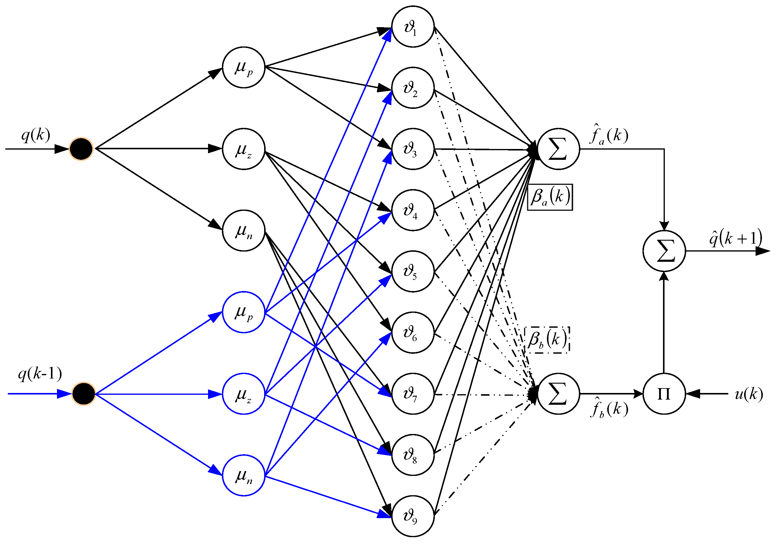
3. Identification of an Equivalent Model

The affine equivalent model of the controlled plant in (2) is defined by

$$q(k+1)=f_a\left(w_k\right)+f_b\left(w_k\right)u\left(k\right),$$

(4)

where $f_a\left(w_k\right)$ and $f_b\left(w_k\right)$ are unknown functions. According to $f_u\left(k\right)$ in (3) and the model in (4), we have

$$f_u\left(k\right)=\frac{\partial q(k+1)}{\partial u\left(k\right)}=f_b\left(w_k\right).$$

(5)

The two functions $f_a\left(w_k\right)$ and $f_b\left(w_k\right)$ in (4) are identified by the adaptive network MiFREN, as illustrated in Figure 2. The estimated output of $\widehat{q}(k+1)$ is obtained as

$$\widehat{q}(k+1)={\widehat{f}}_a\left(k\right)+{\widehat{f}}_b\left(k\right)u\left(k\right),$$

(6)

where ${\widehat{f}}_a\left(k\right)$ and ${\widehat{f}}_b\left(k\right)$ are the estimated functions of $f_a\left(w_k\right)$ and $f_b\left(w_k\right)$, respectively. By using the general relation of MiFREN, the functions ${\widehat{f}}_a\left(k\right)$ and ${\widehat{f}}_b\left(k\right)$ are utilized as

$${\widehat{f}}_a\left(k\right)={\beta }_a^T\left(k\right)\vartheta \left(k\right),$$

(7)

and

$${\widehat{f}}_b\left(k\right)={\beta }_b^T\left(k\right)\vartheta \left(k\right),$$

(8)

where ${\beta }_a\left(k\right)$ and ${\beta }_b\left(k\right)$ are weight parameter vectors, and $\vartheta \left(k\right)$ is the membership vector, as depicted in Figure 2. The network architecture in Figure 2 is designed by a set of IF-THEN rules, such as:

$$IFq(k)ispositiveandq(k+1)ispositiveTHEN{\widehat{f}}_a(k)shouldbepositiveand{\widehat{f}}_b(k)shouldbepositive.$$

In this case, two inputs $q\left(k\right)$ and $q(k+1)$ have three linguistic variables, as the following membership functions: Positive (p), Zero (z), and Negative (n). The design of membership functions will be demonstrated by the experimental system in Section 5.

Next, the online learning scheme for adjustable parameters ${\beta }_a\left(k\right)$ and ${\beta }_b\left(k\right)$ is established with the convergence analysis by the following Theorem.

Lemma 1.

For the equivalent model given by (6)–(8) with the idea weight parameters ${\beta }_a^{\ast }$ and ${\beta }_b^{\ast }$, the convergence of the internal signals ${\tilde{\beta }}_a\left(k\right)={\beta }_a^{\ast }-{\beta }_a\left(k\right)$ and ${\tilde{\beta }}_b\left(k\right)={\beta }_b^{\ast }-{\beta }_b\left(k\right)$, and the approximation error $\widehat{e}(k+1)=q(k+1)-\widehat{q}(k+1)$ can be guaranteed by the tuning laws given by

$${\beta }_a(k+1)={\beta }_a\left(k\right)+{\eta }_h\left(k\right)\widehat{e}(k+1)\vartheta \left(k\right),$$

(9)

and

$${\beta }_b(k+1)={\beta }_b\left(k\right)+{\eta }_h\left(k\right)\widehat{e}(k+1)u\left(k\right)\vartheta \left(k\right),$$

(10)

where the learning rate ${\eta }_h\left(k\right)$ is determined by

$${\eta }_h\left(k\right)=\frac{{\gamma }_h}{\left|\right|{\vartheta }_t\left(k\right){\left|\right|}^2},$$

(11)

with $0<{\gamma }_h<1$.

Proof. 

By combining the tuning laws (9) and (10), we get

$${\beta }_t(k+1)={\beta }_t\left(k\right)+{\eta }_h\left(k\right)\widehat{e}(k+1){\vartheta }_t\left(k\right),$$

(12)

where ${\beta }_t\left(k\right)={\left[{\beta }_a\left(k\right){\beta }_b\left(k\right)\right]}^T$ and ${\vartheta }_t\left(k\right)={\left[\vartheta \left(k\right)\vartheta \left(k\right)u\left(k\right)\right]}^T$. There exists an idea weight parameter ${\beta }_t^{\ast }={\left[{\beta }_a^{\ast }{\beta }_b^{\ast }\right]}^T$ for MiFREN such that

$$q(k+1)={\beta }_t^{\ast T}{\vartheta }_t\left(k\right)+{\epsilon }_h\left(k\right),$$

(13)

where ${\epsilon }_h\left(k\right)$ is the residue error and $|{\epsilon }_h\left(k\right)|\le {\epsilon }_H$ where ${\epsilon }_H$ a positive constant. The approximation error dynamic $\widehat{e}(k+1)$ can be expressed as

$$\begin{array}{lll}\widehat{e}(k+1)& =& q(k+1)-\widehat{q}(k+1),\\ & =& {[{\beta }_t^{\ast }-{\beta }_t\left(k\right)]}^T{\vartheta }_t\left(k\right)+{\epsilon }_h\left(k\right),\\ & =& {\tilde{\beta }}_t^T\left(k\right){\vartheta }_t\left(k\right)+{\epsilon }_h\left(k\right),\end{array}$$

(14)

where ${\tilde{\beta }}_t\left(k\right)={\beta }_t^{\ast }-{\beta }_t\left(k\right)$. Subtraction of ${\beta }_t^{\ast }$ from both sides of the tuning law (12) leads to

$${\tilde{\beta }}_t(k+1)={\tilde{\beta }}_t\left(k\right)-{\eta }_h\left(k\right){\vartheta }_t\left(k\right)\widehat{e}(k+1).$$

(15)

Substitution of (14) into (15) gives

$$\begin{array}{lll}{\tilde{\beta }}_t(k+1)& =& {\tilde{\beta }}_t\left(k\right)-{\eta }_h\left(k\right){\vartheta }_t\left(k\right)[{\tilde{\beta }}_t^T\left(k\right){\vartheta }_t\left(k\right)+{\epsilon }_h\left(k\right)],\\ & =& [I-{\eta }_h\left(k\right){\vartheta }_t\left(k\right){\vartheta }_t^T\left(k\right)]{\tilde{\beta }}_t\left(k\right)-{\eta }_h\left(k\right){\epsilon }_h\left(k\right){\vartheta }_t\left(k\right),\\ & \le & [1-{\eta }_h\left(k\right)\left|\right|{\vartheta }_t{\left(k\right)\left|\right|}^2]{\tilde{\beta }}_t\left(k\right)+{\eta }_h\left(k\right){\epsilon }_H{\vartheta }_t\left(k\right).\end{array}$$

(16)

The second term of the right-hand side of (16) is always bounded. Thus, the convergence of the sequence ${\tilde{\beta }}_t\left(k\right)$ requires

$$-1<1-{\eta }_h\left(k\right)\left|\right|{\vartheta }_t\left(k\right){\left|\right|}^2<1.$$

(17)

By using the learning rate ${\eta }_h\left(k\right)$ from (11), the condition (17) always holds. The convergence proof of internal signals is completed.

Next, the convergence proof of $\widehat{e}\left(k\right)$ is conducted. Let’s define the change of $\widehat{e}\left(k\right)$ as

$$\mathsf{\Delta }\widehat{e}\left(k\right)=\widehat{e}(k+1)-\widehat{e}\left(k\right).$$

(18)

The change in (18) can be approximated by

$$\mathsf{\Delta }\widehat{e}\left(k\right)\approx {\left[\frac{\partial \widehat{e}(k+1)}{\partial {\beta }_t\left(k\right)}\right]}^T\mathsf{\Delta }{\beta }_t\left(k\right).$$

(19)

According to (12), we have

$$\frac{\partial \widehat{e}(k+1)}{\partial {\beta }_t\left(k\right)}={\eta }_h\left(k\right){\vartheta }_t\left(k\right),$$

(20)

and

$$\mathsf{\Delta }{\beta }_t\left(k\right)={\eta }_h\left(k\right){\vartheta }_t\left(k\right))\widehat{e}(k+1).$$

(21)

Substitution of (20) and (21) into (19) leads to

$$\mathsf{\Delta }\widehat{e}\left(k\right)\doteq {\eta }_h^2\left(k\right)\left|\right|{\vartheta }_t\left(k\right){\left|\right|}^2\widehat{e}(k+1).$$

(22)

By setting (18) equal to (22), we have

$$\widehat{e}(k+1)-\widehat{e}\left(k\right)={\eta }_h^2\left(k\right)\left|\right|{\vartheta }_t\left(k\right){\left|\right|}^2\widehat{e}(k+1),$$

(23)

and

$$\widehat{e}(k+1)=\frac{1}{1-{\eta }_h^2\left(k\right)\left|\right|{\vartheta }_t\left(k\right){\left|\right|}^2}\widehat{e}\left(k\right).$$

(24)

The convergence of the sequence $\widehat{e}\left(k\right)$ in (24) can be guaranteed when

$$-1<\frac{1}{1-{\eta }_h^2\left(k\right)\left|\right|{\vartheta }_t\left(k\right){\left|\right|}^2}<1.$$

(25)

By using the learning rate in (11), the condition in (25) always holds. The convergence proof of the approximation error is completed.  □

Utilizing the equivalent model given by (6)–(8), the controller will be established by another MiFREN in the next section.

4. MiFREN Adaptive Control and Closed-Loop Analysis

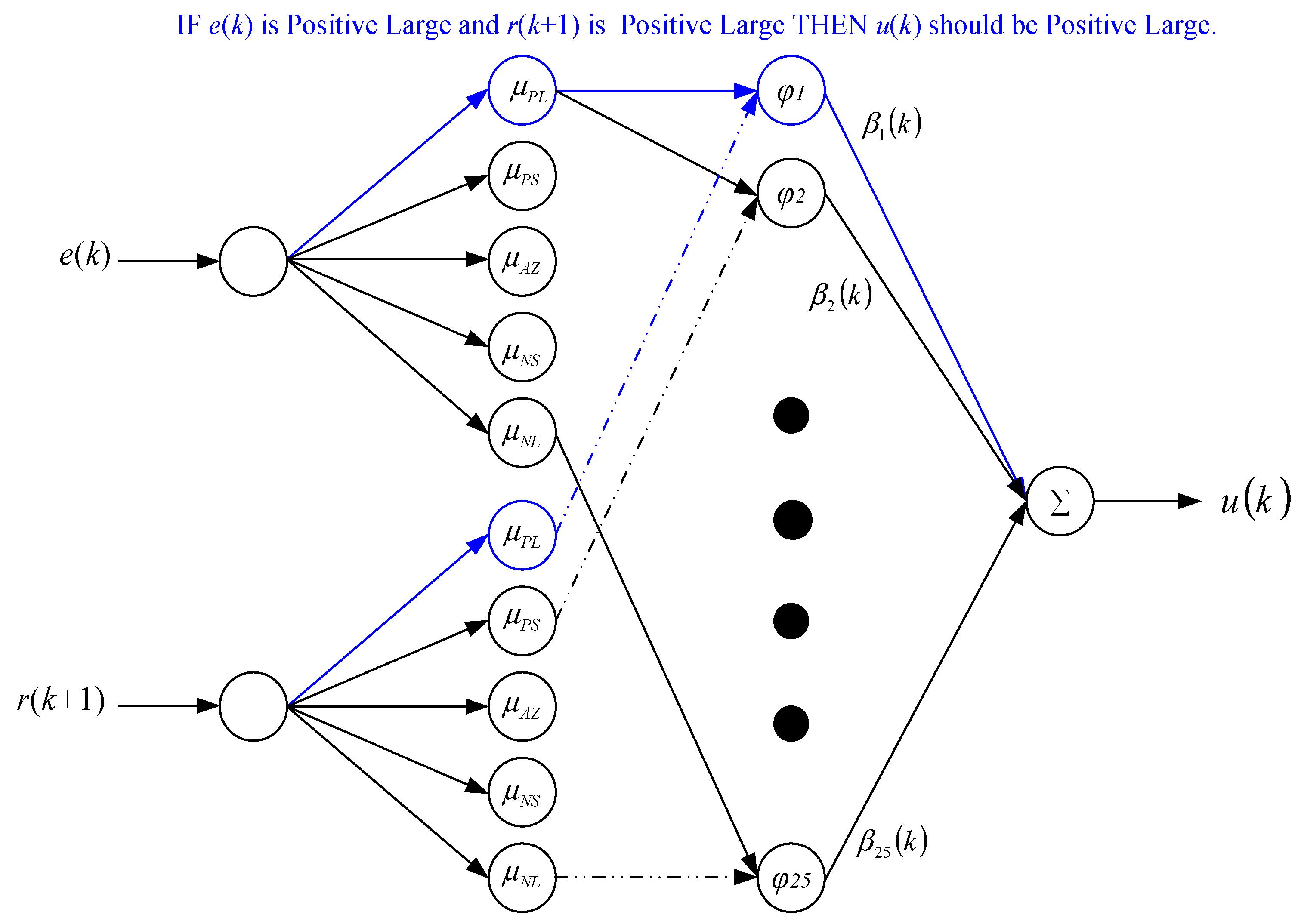
4.1. MiFREN Adaptive Controller

Another MiFREN is established for the design of the controller. The purpose of the controller is to generate the control effort $u\left(k\right)$ that forces the system to follow the desired trajectory $r(k+1)$. For the class of discrete-time systems given by (1) and (2), some essential assumptions are stated, as follows:

Assumption 2.

There exists an idea control effort $u^{\ast }\left(k\right)$ for the controlled plant (1) and (2), such that $r(k+1)=f(w\left(k\right),u^{\ast }\left(k\right))$ and and $r(k+1)$ are known in advance.

Assumption 3.

There exists an idea weight parameter ${\beta }^{\ast }\in {\mathbb{R}}^F$ for MiFREN, where F denotes the number of IF-THEN rules for the network structure, such that

$$u^{\ast }\left(k\right)={\beta }^{\ast T}\phi \left(k\right)+{\epsilon }_u\left(k\right),$$

(26)

where ${\phi }^T\left(k\right)\in {\mathbb{R}}^F$ is the regressive vector from the rule interface of MiFREN and ${\epsilon }_u\left(k\right)$ is the residue error, where $|{\epsilon }_u\left(k\right)|\le {\epsilon }_M$.

Remark 1.

Assumption 2 is very general for the design of adaptive controllers, and Assumption 3 is the universal function approximation of MiFREN [18].

For the negative feedback of the output $q\left(k\right)$, the tracking error $e\left(k\right)$ is defined by

$$e\left(k\right)=r\left(k\right)-q\left(k\right).$$

(27)

The practical control effort $u\left(k\right)$ is utilized by MiFREN as

$$u\left(k\right)={\beta }^T\left(k\right)\phi \left(k\right),$$

(28)

where $\beta \left(k\right)\in {\mathbb{R}}^F$ denotes the weight parameters and $\phi \left(k\right)$ is a regressive vector for the IF-THEN rules of the tracking error and the desired trajectory. In general, the vector $\phi \left(k\right)$ can be expressed as

$$\phi \left(k\right)={[{\mu }_{e1}\left(e_k\right){\mu }_{r1}\left(r_{k+1}\right),\cdots ,{\mu }_{ei}\left(e_k\right){\mu }_{ri}\left(r_{k+1}\right),\cdots ,{\mu }_{eF}\left(e_k\right){\mu }_{rF}\left(r_{k+1}\right)]}^T,$$

(29)

where ${\mu }_{ei}(-)$ and ${\mu }_{ri}(-)$ are the membership functions of e and r for the ith rule, respectively.

The IF-THEN rules are established by the relation between the tracking error and the desired trajectory, such that:

IF e(k) is Positive Large AND r(k + 1) is Positive Large THEN u(k) should be Positive Large.

Each of the inputs $e\left(k\right)$ and $r(k+1)$ have five membership functions: Positive Large (PL), Positive Small (PS), Almost Zero (AZ), Negative Small (NS), and Negative Large (NL). This leads to 25 IF-THEN rules. Figure 3 represents the network architecture of MiFREN for the controller design.

4.2. Adaptive Algorithm and Closed Loop Analysis

An adaptive algorithm will be established to tune the adjustable parameters $\beta \left(k\right)$ under the consideration of closed-loop performance and stability analysis. By using the dead-zone function, the adaptive algorithm is proposed as

$$\beta (k+1)=\beta \left(k\right)+\frac{\eta \left(k\right)}{{\overline{\gamma }}_u{\left|\right|\phi \left(k\right)\left|\right|}^2}{e}_{k+1}\phi \left(k\right),$$

(30)

where $\eta \left(k\right)$ is the time-varying learning rate and ${\overline{\gamma }}_u$ is a constant, which will be discussed below.

The learning rate plays an importance role of the controller performance. The following theorem manifests the selection of the learning rate, regarding the closed loop analysis.

Theorem 1.

For the control law (28) with the adaptive algorithm (30) applyied to the discrete-time systems (1) and (2), the convergence of tracking error and internal signals can be guaranteed when the learning rate is given as

$$\eta \left(k\right)=\frac{{\overline{\gamma }}_u}{{\widehat{f}}_b\left(k\right)+{\epsilon }_o}<\frac{{\overline{\gamma }}_u}{{\epsilon }_o},$$

(31)

where

$$0<{\overline{\gamma }}_u\le {\epsilon }_o,$$

(32)

and

$$0<{\overline{f}}_u\le {\overline{\gamma }}_u.$$

(33)

Remark 2.

Practically, ${\overline{\gamma }}_u$ is unknown and, thus, it can be approximated by ${\overline{\gamma }}_u=C_{u}max\{{\widehat{f}}_b\left(k\right)\}$, where $1\le C_u$.

Proof. 

The proof is conducted with two parts. The first part is to prove the convergence of the internal signals ${\tilde{\beta }}^T\left(k\right)$ when $\tilde{\beta }\left(k\right)={\beta }^{\ast }-\beta \left(k\right)$. Subtraction of ${\beta }^{\ast }$ from both sides of (30) leads to

$$\tilde{\beta }(k+1)=\tilde{\beta }\left(k\right)-\frac{\eta \left(k\right)}{{\overline{\gamma }}_u{\left|\right|\phi \left(k\right)\left|\right|}^2}{e}_{k+1}\phi \left(k\right).$$

(34)

By using (27) with (26) and (28), the error dynamic can be rearranged as

$$\begin{array}{lll}e(k+1)& =& r(k+1)+q(k+1),\\ & =& f(w\left(k\right),u^{\ast }\left(k\right))-f(w\left(k\right),u\left(k\right)),\\ & =& \frac{\partial f\left(w\right(k),\nu )}{\partial \nu }{|}_{\nu =u_c\left(k\right)}\left[u^{\ast }\left(k\right)-u\left(k\right)\right],\end{array}$$

(35)

$$\begin{array}{cc}=& {\gamma }_{uc}\left(k\right){\tilde{\beta }}^T\left(k\right)\phi \left(k\right)+{\gamma }_{uc}\left(k\right){\epsilon }_u\left(k\right),\hfill \end{array}$$

(36)

where

$${\gamma }_{uc}\left(k\right)=\frac{\partial f\left(w\right(k),\nu )}{\partial \nu }{|}_{\nu =u_c\left(k\right)},$$

(37)

with $u_c\left(k\right)\in [\min (u_k^{\ast },u_k),\max (u_k^{\ast },u_k)]$. Substitution of (35) into (34) gives

$$\tilde{\beta }(k+1)=\left[I-\eta \left(k\right)\frac{{\gamma }_{uc}\left(k\right)}{{\overline{\gamma }}_u}\right]\tilde{\beta }\left(k\right)-{\epsilon }_B\left(k\right),$$

(38)

where

$${\epsilon }_B\left(k\right)=\frac{\eta \left(k\right){\gamma }_{uc}(k}{{\overline{\gamma }}_u{\left|\right|\phi \left(k\right)\left|\right|}^2}{\epsilon }_u\left(k\right)\phi \left(k\right).$$

(39)

According to (31) and as $|{\epsilon }_u\left(k\right)|\le {\epsilon }_M$, we have that ${\epsilon }_B\left(k\right)$ in (39) is clearly bounded. Thus, the convergence of (38) can be guaranteed when

$$|1-\eta \left(k\right)\frac{{\gamma }_{uc}\left(k\right)}{{\overline{\gamma }}_u}|<1.$$

(40)

By using the learning rate in (31), it’s clear that the condition in (40) always holds. The convergence proof of the internal signals $\beta \left(k\right)$ is completed.

The second part is to prove the convergence of the tracking error $e\left(k\right)$. By using the chain rule, we have

$$\begin{array}{lll}\frac{\partial e(k+1)}{\partial \beta \left(k\right)}& =& \frac{\partial e(k+1)}{\partial q(k+1)}\frac{\partial q(k+1)}{\partial u\left(k\right)}\frac{\partial u\left(k\right)}{\partial \beta \left(k\right)},\\ & =& -f_u\left(k\right)\phi \left(k\right),\end{array}$$

(41)

where

$$f_u\left(k\right)=\frac{\partial q(k+1)}{\partial u\left(k\right)}=\frac{\partial f\left(w\right(k),u(k\left)\right))}{\partial u\left(k\right)}.$$

(42)

With the equivalent model (7), it is clear that

$$f_u\left(k\right)=\frac{\partial \widehat{q}(k+1)}{\partial u\left(k\right)}={\widehat{f}}_b\left(k\right).$$

(43)

By using (41), the change of tracking error $\mathsf{\Delta }e\left(k\right)$ can be approximated by

$$\begin{array}{lll}\mathsf{\Delta }e\left(k\right)& =& e(k+1)-e\left(k\right),\\ & \approx & {\left[\frac{\partial e(k+1)}{\partial \beta \left(k\right)}\right]}^T\mathsf{\Delta }\beta \left(k\right),\\ & =& -{\widehat{f}}_b\left(k\right){\phi }^T\left(k\right)\mathsf{\Delta }\beta \left(k\right).\end{array}$$

(44)

Referring to the adaptive algorithm in (30), it is clear that

$$\begin{array}{lll}\mathsf{\Delta }\beta \left(k\right)& =& \beta (k+1)-\beta \left(k\right),\\ & =& \frac{\eta \left(k\right)}{{\overline{\gamma }}_u{\left|\right|\phi \left(k\right)\left|\right|}^2}{e}_{k+1}\phi \left(k\right).\end{array}$$

(45)

Substitution of (45) into (44) gives

$$\mathsf{\Delta }e\left(k\right)=-\eta \left(k\right)\frac{{\widehat{f}}_b\left(k\right)}{{\overline{\gamma }}_u}e(k+1).$$

(46)

Thereafter, the relation in (46) can be rearranged as

$$\begin{array}{ccc}\hfill e(k+1)-e\left(k\right)& =& -\eta \left(k\right)\frac{{\widehat{f}}_b\left(k\right)}{{\overline{\gamma }}_u}e(k+1),\hfill \\ \hfill e(k+1)& =& \frac{1}{1+\eta \left(k\right)\frac{{\widehat{f}}_b\left(k\right)}{{\overline{\gamma }}_u}}e\left(k\right).\hfill \end{array}$$

(47)

For the convergence of the sequence in (47), it is required that

$$\left|\frac{1}{1+\eta \left(k\right)\frac{{\widehat{f}}_b\left(k\right)}{{\overline{\gamma }}_u}}\right|<1.$$

(48)

By using the learning rate in (31), it’s clear that the condition in (48) always holds. The convergence proof of the tracking error is completed.  □

The validation of the proposed control scheme and the setting of the designed parameters and membership functions will be addressed in the following section.

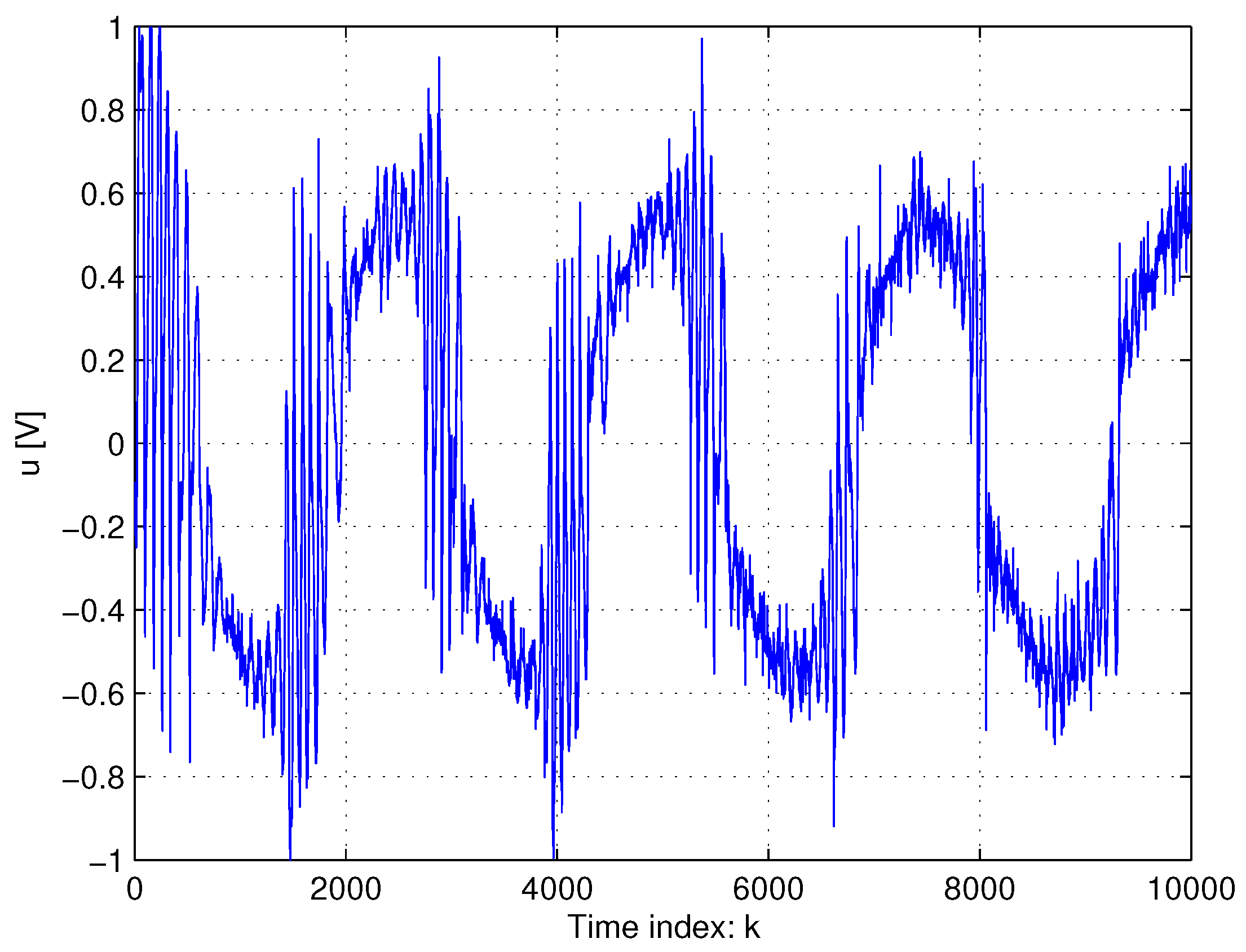
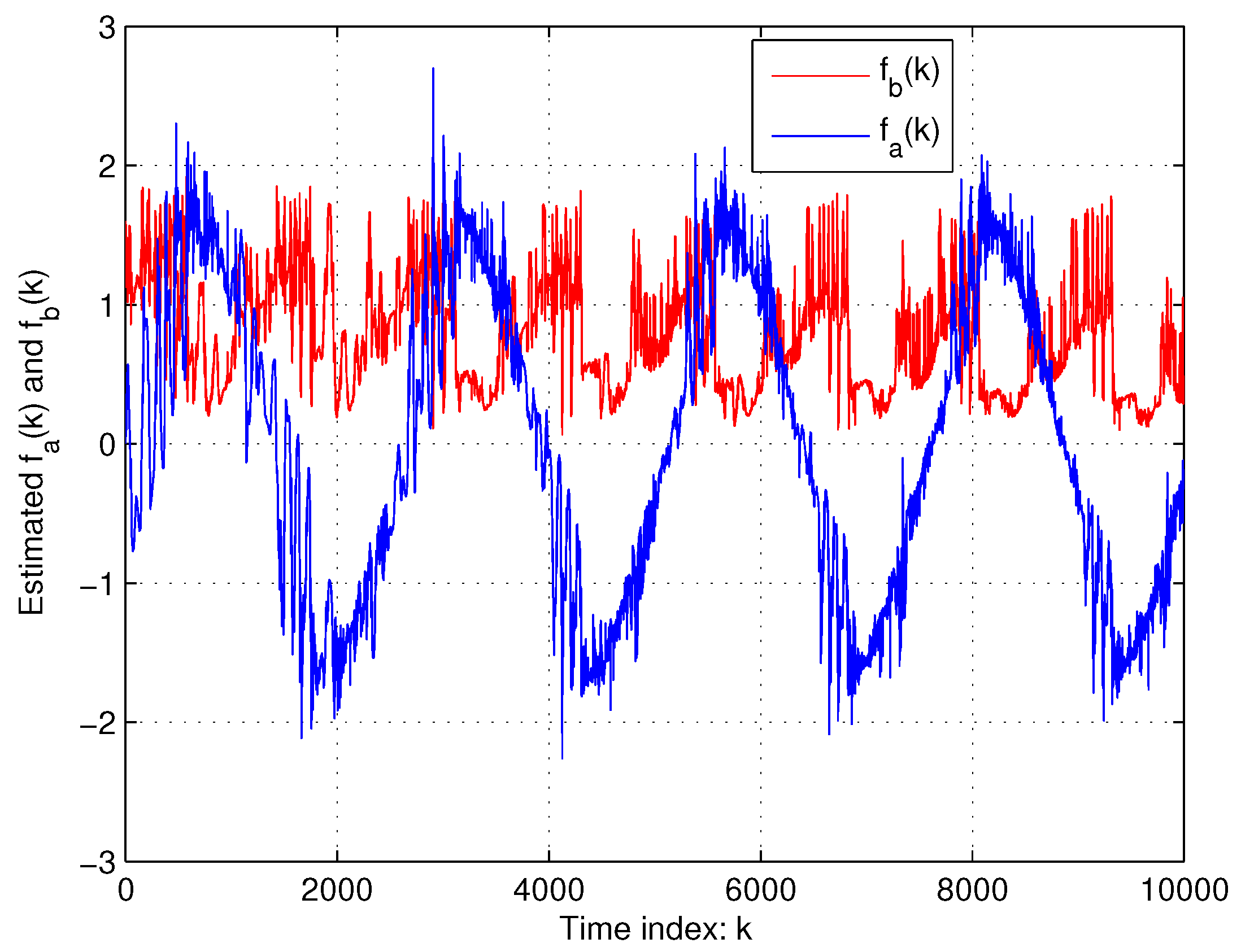
5. Experimental Results

This experimental system with the robotic arm ABB model IRB-1400 is constructed using the configuration mentioned in Section 2. The membership functions for MiFREN identification are given in Figure 4, and cover the robotic operating range $\pm 2$ Rad. The membership functions for the tracking error $e\left(k\right)$ and the desired position $r(k+1)$ of the MiFREN controller are shown in Figure 5. The designed parameters are given as ${\gamma }_h=0.5$, ${\epsilon }_o=2.15$, and $C_u=1.05$.

The tracking performance and the tracking error are illustrated in Figure 6 and the control effort is shown in Figure 7. The control signal contains the high-frequency components which compensate for the non-linearities. The estimated functions ${\widehat{f}}_a\left(k\right)$ and ${\widehat{f}}_b\left(k\right)$ are presented in Figure 8. The learning rate ${\eta }_h\left(k\right)$, given by Lemma 1, is shown in Figure 9. In Figure 10, the plots of $\left|\right|{\beta }_a{\left|\right|}^2$ and $\left|\right|{\beta }_b{\left|\right|}^2$ are given to demonstrate the convergence of the internal signals in the MiFREN equivalent model. From the plot of ${\widehat{f}}_b\left(k\right)$ in Figure 8, it’s clear that the maximum of ${\widehat{f}}_b\left(k\right)$ is around 2, or

$$max\left\{{\widehat{f}}_b\left(k\right)\right\}\approx 2.$$

(49)

Referring to the remark following Theorem 1, and as $C_u=1.05$, the parameter ${\overline{\gamma }}_u$ can be determined by

$$\begin{array}{lll}{\overline{\gamma }}_u& =& C_{u}max\left\{{\widehat{f}}_b\left(k\right)\right\},\\ & =& 1.05\times 2=2.1.\end{array}$$

(50)

By setting ${\epsilon }_o=2.15$, we have ${\overline{\gamma }}_u\le {\epsilon }_o$. Thus, the condition (32) of Theorem 1 has been completely fulfilled. Thereafter, the learning rate of the MiFREN controller is shown in Figure 11 and the convergence of the weight parameters is displayed in Figure 12.

The comparison results with other MFAC schemes are given next. For the case of Controller A, the DDC scheme, developed by the results in [9,13], is implemented for the robotic systems when the designed parameter ${\gamma }_u$ in (14) of [13] is given as ${\gamma }_u=0.5$ and the membership functions of $e\left(k\right)$ are defined as the same as in Figure 5 for the proposed controller. The tracking performance is presented by the plots in Figure 13, and the sum square error (SSE) is 24.9450, where the SSE is defined by

$$\mathrm{SSE}=\sum _{k=1}^{k_{\max }}{e}^2\left(k\right),$$

(51)

with $k_{\max }=$ 10,000. Controller B is established by using the strong Kalman filter proposed in [10]. In this application, the input is converted to be the joint velocity for the estimated Jacobian matrix. The tracking performance is shown in Figure 14, and the SSE value is 18.7044. A PID controller, based on a fourth-order infinite impulse response filter and developed in [6], is selected as Controller C. For all of the six joints of the robot, the controller parameters are given in

Table 1. Parameter settings for Controller C [6].

Joint	${\mathit{K}}_{\mathit{p}}$	${\mathit{T}}_{\mathit{i}}$	${\mathit{T}}_{\mathit{d}}$
1	5.26	0.36	0.11
2	8.74	0.27	0.11
3	13.91	0.21	0.17
4	2.72	0.11	0.14
5	6.83	0.13	0.12
6	4.85	0.07	0.12

. Figure 15 displays the tracking performance of Controller C, and the SEE value is 96.2553.

Table 2. Comparison Results.

Controller	SSE	Remark
A: [9,13]	24.9450	Figure 13
B: [10]	18.7044	Figure 14
C: [6]	96.2553	Figure 15
Proposed controller	6.1437	Figure 6

concludes the comparison results.

6. Conclusions

An open-architecture robot with VFD and a task-multiplexer has been considered as a class of unknown discrete-time systems. By using only the input/output data set of the robotic system, the equivalent model has been developed by MiFREN, where the convergence of the model error and adjustable parameter have been established. Another MiFREN has been established as the adaptive controller, where the IF-THEN rules have been defined by using general human knowledge of the robotic system. The proposed controller is completely model-free where the convergence of the tracking error is definitely guaranteed. Thereafter, the performance of the closed-loop system has been clearly demonstrated through both theoretical and practical aspects. The comparison results with well-known robotic controllers and recent approaches have shown the advantage of the proposed scheme. Development of the task-multiplexer and control high-frequency reduction are efforts to be addressed in our future investigations.

References

1. Mohammad, A.-E.K.; Hong, J.; Wang, D. Design of a force-controlled end-effector with low-inertia effect for robotic polishing using macro-mini robot approach. Robot. Comput. Integr. Manuf. 2018, 49, 54–65. [Google Scholar] [CrossRef]
2. Zheng, M. Control Framework for a Macro/Mini Manipulator. Ph.D. Thesis, National University of Singapore, Singapore, 2018. [Google Scholar]
3. Wang, H.; Jiang, N.; Liu, T.; Cao, Y. Adaptive stable control of manipulator system based on immersion and invariance. Math. Model. Anal. 2018, 23, 379–389. [Google Scholar] [CrossRef]
4. Markus, E.D.; Agee, J.T.; Jimoh, A.A. Flat control of industrial robotic manipulators. Robot. Auton. Syst. 2017, 87, 226–236. [Google Scholar] [CrossRef]
5. Sankar, S.; Tsai, C.Y. ROS-based human detection and tracking from a wireless controlled mobile robot using kinect. Appl. Syst. Innov. 2019, 2, 5. [Google Scholar] [CrossRef]
6. Martinez-Prado, M.A.; Resendiz, J.R.; Gomez-Loenzo, R.A.; Herrera-Ruiz, G.; Franco-Gasca, L.A. An FPGA-Based open architecture industrial robot controller. IEEE Access 2018, 6, 13407–13417. [Google Scholar] [CrossRef]
7. Alabdo, A.; Javier, P.; Garcia, G.J.; Pomares, J.; Torres, F. FPGA-based architecture for direct visual control robotic systems. Mechatronics 2016, 39, 204–216. [Google Scholar] [CrossRef]
8. Treesatayapun, C. A data-driven adaptive controller for a class of unknown nonlinear discrete-time systems with estimated PPD. Eng. Sci. Technol. Int. J. 2015, 18, 218–228. [Google Scholar] [CrossRef]
9. Zhu, Y.; Hou, Z.S. Data-driven MFAC for a class of discrete-time nonlinear systems with RBFNN. IEEE Trans. Neural Netw. Learn. Syst. 2014, 25, 1013–1020. [Google Scholar] [PubMed]
10. Minhan, L.; Rongjie, K.; Branson, D.T.; Dai, J.S. Model-free control for continuum robots based on an adaptive Kalman filter. IEEE/ASME Trans. Mechatron. 2018, 23, 286–297. [Google Scholar]
11. Chi, R.; Hou, Z.; Jin, S. A data-driven adaptive ILC for a class of nonlinear discrete-time systems with random initial states and iteration-varying target trajectory. J. Frankl. Inst. 2015, 352, 2407–2424. [Google Scholar] [CrossRef]
12. Bu, X.; Qiao, Y.; Hou, Z.; Yang, J. Model free adaptive control for a class of nonlinear systems using quantized information. Asian J. Control 2018, 20, 1–7. [Google Scholar] [CrossRef]
13. Treesatayapun, C. Data input-output adaptive controller based on IF-THEN rules for a class of non-affine discrete-time systems: The robotic plant. J. Intell. Fuzzy Syst. 2015, 28, 661–668. [Google Scholar]
14. Treesatayapun, C. Adaptive control based on IF-THEN rules for grasping force regulation with unknown contact mechanism. Robot. Comput. Integr. Manuf. 2014, 30, 11–18. [Google Scholar] [CrossRef]
15. Chen, C.; Wen, C.; Liu, Z.; Xie, K.; Zhang, Y.; Philip-Chen, C.L. Adaptive consensus of nonlinear multi-agent systems with non-identical partially unknown control directions and bounded Modelling errors. IEEE Trans. Autom. Control 2017, 62, 4654–4659. [Google Scholar] [CrossRef]
16. Sarangapani, J. Neural Network Control of Nonlinear Discrete-Time Systems; CRC Press: New York, NY, USA, 2006. [Google Scholar]
17. Hosseinzadeh, S.; Larijani, H.; Curtis, K.; Wixted, A. An adaptive neuro-fuzzy propagation model for LoRaWAN. Appl. Syst. Innov. 2019, 2, 10. [Google Scholar] [CrossRef]
18. Treesatayapun, C.; Uatrongjit, S. Adaptive controller with Fuzzy rules emulated structure and its applications. Eng. Appl. Artif. Intell. 2005, 18, 603–615. [Google Scholar] [CrossRef]
19. Beechner, T.L.; Carpenter, A.L. A >98% efficient >150 kRPM high-temperature liquid-cooled SiC VFD for hybrid-electric turbochargers. In Proceedings of the 2017 IEEE Applied Power Electronics Conference and Exposition (APEC), Tampa, FL, USA, 26–30 March 2017; pp. 3674–3680. [Google Scholar]
20. Shenoy, P.; Solis, O.; Zheng, L. Commereializing medium voltage VFD that utilizes high voltage SiC technology. In Proceedings of the 2017 IEEE International Workshop on Integrated Power Packaging (IWIPP), Delft, The Netherlands, 5–7 April 2017. [Google Scholar]
21. Guo, C.; Zhang, A.; Zhang, H.; Zhang, L. Adaptive backstepping control with online parameter estimator for a plug-and-play parallel converter system in a power switcher. Energies 2018, 11, 3528. [Google Scholar] [CrossRef]
22. Das, K.; Srinivas, M.N.; Madhusudanan, V.; Pinelas, S. Mathematical analysis of a prey–predator system: An adaptive back-stepping control and stochastic approach. Math. Comput. Appl. 2019, 24, 22. [Google Scholar] [CrossRef]
23. Rodriguez, M.D.; Valera, A.; Mata, V.; Valles, M. Model-based control of a 3-DOF parallel robot based on identified relevant parameters. IEEE/ASME Trans. Mechatron. 2013, 18, 1737–1744. [Google Scholar] [CrossRef]
24. Yang, X.; Ge, S.S.; Liu, J. Dynamics and noncollocated model-free position control for a space robot with multi-link flexible manipulators. Asian J. Control 2019, 21, 1–11. [Google Scholar] [CrossRef]
Figure 1. Discrete-time robotic control system block diagram. VFD, variable-frequency drive.
Asi 02 00012 g001
Figure 2. MiFREN identification model.
Asi 02 00012 g002
Figure 3. Multi-input Fuzzy Rule Emulated Network (MiFREN) Controller with an IF-THEN rule.
Asi 02 00012 g003
Figure 4. Membership functions of the MiFREN equivalent model: q ( k ) and q ( k 1 ) .
Asi 02 00012 g004
Figure 5. Membership functions of the MiFREN controller: e ( k ) and r ( k + 1 ) .
Asi 02 00012 g005
Figure 6. Tracking performance: q ( k ) and e ( k ) .
Asi 02 00012 g006
Figure 7. Control effort: u ( k ) .
Asi 02 00012 g007
Figure 8. Estimated functions: f ^ a ( k ) and f ^ b ( k ) .
Asi 02 00012 g008
Figure 9. Learning rate of the MiFREN equivalent model: η h ( k ) .
Asi 02 00012 g009
Figure 10. Weight parameters of the MiFREN equivalent model.
Asi 02 00012 g010
Figure 11. Learning rate of the MiFREN controller: η ( k ) .
Asi 02 00012 g011
Figure 12. Weight parameters of the MiFREN controller.
Asi 02 00012 g012
Figure 13. Tracking performance: Controller A.
Asi 02 00012 g013
Figure 14. Tracking performance: Controller B.
Asi 02 00012 g014
Figure 15. Tracking performance: Controller C.
Asi 02 00012 g015