A Taphonomic Study of DS-22A (Bed I, Olduvai Gorge) and Its Implications for Reconstructing Hominin-Carnivore Interactions at Early Pleistocene Anthropogenic Sites

Abstract

The longstanding debate over early hominin subsistence strategies, particularly the hunting-versus-scavenging hypothesis, as well as discussions regarding the functionality of Oldowan sites, has been primarily centered on the archeological and paleoanthropological record of Olduvai Gorge. Historically, FLK Zinj has been at the core of these debates, serving as a principal empirical reference due to the prevailing assumption that most other Bed I sites at Olduvai represented non-anthropogenic accumulations However, recent discoveries have significantly reshaped this perspective. Newly identified early sites, including PTK, DS, and AGS, situated within the paleolandscape and thin stratigraphic context of FLK Zinj, provide crucial new anthropogenic datasets. These sites offer additional dimensions to the study of early hominin behavior, facilitating a more nuanced reconstruction of their adaptive strategies in this paleoenvironment. Furthermore, methodological advancements in recent years—including controlled experimental and actualistic studies, sophisticated statistical modeling, and the integration of machine learning algorithms—have greatly enhanced the analytical frameworks available for investigating early hominin behavior. These innovations have refined the ability to formulate and test hypotheses within a rigorous scientific paradigm, significantly improving the resolution of archeological and taphonomic interpretations. This study presents an in-depth taphonomic analysis of the faunal assemblage from level 22A at DS, a Bed I site at Olduvai Gorge dated to approximately 1.84 Ma. The assemblage exhibits exceptional preservation, enabling detailed assessments of skeletal part representation, fragmentation patterns, and surface modifications. By combining traditional taphonomic methodologies with state-of-the-art AI-driven bone surface modification (BSM) analyses, this research contributes novel insights into the interactions between early hominins and carnivores, elucidating the complex ecological dynamics of an Early Pleistocene African paleolandscape.

1. Introduction

• Olduvai Gorge and its role in the reconstruction of early human behavior.

Olduvai Gorge, situated to the southeast of the Serengeti Plains in northern Tanzania, is renowned for its rich fossil discoveries, especially in relation to early hominins and their stone tool behaviors, and stands as a key area for the study of human evolution [1]. Over the last 200,000 years, fluvial erosion has intricately carved through diverse geological layers, giving rise to the Gorge’s two branches: the primary and secondary gorges. Hay delineated various geological units within Olduvai Gorge [2], forming the basis for contemporary geological investigations. These units include Beds I, II, III, IV, and the Masek, Ndutu, and Naisiusiu Beds. The sites found in Bed I, formally classified as Oldowan, based on their cobble and flake technology [3], have constituted the basis for the reconstruction of early hominin behavior for more than half a century [3,4,5,6,7,8,9]. It is there that one of the most confrontational debates used the Bed I archeological record as a testing ground for multiple hypotheses of early human behavioral evolution [4,5,8,9,10,11,12,13,14,15,16,17,18].

Many experts argue that early access to carcasses would be equivalent to regular meat eating, food sharing, and the development of cooperative strategies, and this could have played a critical role in shaping the human brain and anatomy [4,5,17,19,20,21,22,23,24,25,26,27,28,29,30]. On the other hand, secondary access to defleshed carcasses would imply limited access to animal resources, which could be indicative of the probable absence of food-sharing and other associated complex behaviors.

In recent years, this debate has been fueled by the discovery of new sites and additional evidence that have made our perception and understanding of early humans more complex [31,32,33,34,35].

• DS: an exceptional Early Pleistocene anthropogenic site.

DS, located in Bed I, was discovered in 2014 in the junction between the main and secondary gorges, only a few hundred meters away from its contemporary referent FLK Zinj and right below a dirt road traditionally considered a transit area [36,37,38,39]. This discovery, framed within a specific survey method using past information on site distribution and associated lithofacies, was the result of the erosion of the deposit where it was located, which made the immediate excavation of the area necessary in order to avoid any further loss of materials. At first, an area of 370 m² was opened, reaching an extension of around 560 m² by 2018, which makes DS the largest anthropogenic Early Pleistocene Oldowan site documented at present [37,38,39]. DS, as well as FLK Zinj, PTK, or AGS (all of them Bed I sites), traces its origins to the thin clay layer beneath the 1.84 Ma Tuff 1C, which encompasses two distinct archeological levels or paleosols, both approximately 10 cm thick and deposited under very low-energy conditions: level 22A, characterized by a dark olive-gray (5Y 3/2) earthy clay, and level 22B, which consists of a waxier and darker (olive 5Y 4/2) clay [2,31,40,41,42]. The taphonomic study of the DS 22B level, the largest Early Pleistocene site in Africa, uncovered a faunal assemblage dominated by prime adult and late juvenile animals belonging to Kobus sigmoidalis, Parmularius altidens, Connochaetes sp., Tragelaphus strepsiceros, Megalotragus sp., and Antidorcas recki. The study of the fabric and bone particle size distribution showed that the site was in its depositional locus and unaffected by the slow-energy sedimentary depositional process. In small carcasses (i.e., Antidorcas), all durable skeletal parts are represented similarly (with preservation biases towards the axial skeleton), which suggests that they were transported complete to the site. In contrast, medium-sized carcasses are represented unevenly by anterior and posterior limb bones, with front limbs being more abundant than hind limbs and a clear underrepresentation of axial parts. As shown by Cobo-Sánchez et al. [39] and Domínguez-Rodrigo et al. [43], density-mediated attrition affects axial remains especially but is not the only factor that produces the reverse pattern in medium-sized carcasses. There is an overwhelming signal of bone green breaking, and machine learning analyses on the assemblage, combining the bone fracture pattern and notch type distribution, suggest a scenario in which most of the fracturing (around 90%) was clearly the result of anthropogenic agency [39]. This is further supported by the frequency of percussion marks. There are very few tooth marks, fewer than expected if carnivores (regardless of type) had intervened in the carcass consumption prior to hominins. The cut-mark frequency and anatomical distribution indicated that the hominin-targeted bulk defleshing and all butchering behaviors, including evisceration, are represented in the DS archeofaunal assemblage. Altogether, this suggested that hominins had primary access to most small- and medium-sized carcasses, although occasionally, they might have been able to opportunistically exploit some large carcasses acquired by felids [39,43]. This would suggest that the taphonomic signal imprinted by non-primate carnivores on bone should predominantly indicate hyenid agency and only marginally felid agency too. This is precisely what computer vision methods indicated. By applying computer vision to the bones bearing tooth marks, the study provided robust evidence that early hominins had primary access to meat resources, with hyenas playing a secondary role in bone modification [43].

During the more than 500 m² of excavation of level 22B at DS, the density of 22A was very low and mostly suggested a natural background scatter with an abundant deposition of non-mammal fauna, including turtles (Figure 1). However, upon completion of the excavation, on its southwestern corner, a denser cluster of bones and stone tools started to emerge on the level 22A paleosurface, suggesting probable hominin agency. This prompted the renewal of the (ongoing) excavation and required a preliminary taphonomic analysis of this limited assemblage. Taphonomically supported anthropogenic sites are very scarce during the Early Pleistocene. For this reason, determining the anthropogenic signature of DS 22A is important. Therefore, the present study focuses on the faunal remains recovered from layer 22A from 2015 to 16, positioned within the same paleosurface as FLK Zinj. This study is presented as preliminary, with the simple goal of assessing its potential anthropogenic agency, in anticipation of the complete study once the site is completely excavated and the archeofaunal assemblage is completely exposed.

2. Materials and Methods

The methodology employed in this study integrates traditional taphonomic approaches with advanced AI techniques, offering a novel framework for analyzing BSM.

Taphonomic research on bone surface modifications (BSMs) has played a crucial role in interpreting the fossil record and determining the agent(s) responsible for site formation, e.g., [9,44,45,46,47,48,49,50,51,52,53,54,55,56]. Traditional taphonomic methods provide essential insights into the formation and alteration of archeological and paleontological assemblages. However, their application to BSM analysis is often constrained by methodological equifinality—where distinct taphonomic agents produce similar modifications—and by observer-dependent biases stemming from variability in analytical protocols, quantification methods, and researcher expertise [52,53,54,55,56,57,58,59,60,61,62,63,64]. Although certain criteria have been established to enable BSM identification, e.g., [58,59,60], there is no true consensus, which constitutes a research bias.

Thus, in recent years, more objective methods based on more systematic and statistical analyses have been developed. Among these methods, automatic image classification through machine learning algorithms has shown enormous potential, since it avoids subjectivity in study and interpretation [65,66,67,68,69,70,71,72,73,74]. Although computer vision tasks have proven to be very effective in processing, analyzing, and understanding digital images, there are still few studies in which this methodology has been applied to actual archeological assemblages [39,75], DS being the only early taphonomically supported anthropogenic site where they have been implemented [39].

The incorporation of AI-driven analysis, particularly computer vision (CV) and deep learning (DL) models, enhances pattern recognition capabilities and facilitates a more objective, probabilistic approach to BSM classification. These methodologies have been instrumental in distinguishing, for example, between carnivore-specific tooth-mark morphologies [70,71,72,73,74] and differentiating cut marks produced on fleshed versus defleshed bones [57]. Furthermore, AI models have also demonstrated efficacy in distinguishing pristine experimental cut marks from those altered by trampling or chemical processes [76].

The previous applications of CV and DL models to fossil assemblages have primarily focused on carnivore agency detection and comparative validation against traditional taphonomic interpretations. For instance, at the 1.8 Ma site of DS (Olduvai Gorge, Tanzania), traditional taphonomic analysis identified hominins as the primary agents of site formation, with secondary modification by hyenids [38]. The subsequent DL analysis of carnivore-modified remains confirmed an overwhelming record of hyena-induced modifications [63]. Similarly, at FLK North (Olduvai Gorge, Tanzania), traditional analyses suggested that medium-sized felids had primary access to carcasses, followed by secondary access by hyenas, with minimal to no hominin involvement [1]. DL models corroborated this interpretation, attributing the majority of carnivore modifications to leopards and hyenas while reducing the hominin signal to near non-existence [75].

AI-based methodologies have also been successfully applied beyond Olduvai Gorge. The faunal assemblage from the Upper Pleistocene Tritons Cave (Lleida, Spain) was traditionally attributed to leopard accumulation [77], a conclusion later confirmed through DL-based classification [78]. Similarly, at Toll Cave (Barcelona, Spain), traditional taphonomic analyses indicated that the site functioned as a cave bear hibernation den, with evidence of carnivore scavenging [79]. The application of DL models trained on multiple carnivore taxa, including bears, identified a predominance of bear modifications in the assemblage [80].

Most of the above examples targeted agency identification through the use of tooth marks. Only in one site were cut marks also targeted using AI methods before the present study. The identification of some cut marks on a hyena phalanx from the Upper Pleistocene Navalmaillo shelter (Madrid, Spain), using traditional multivariate microscopic criteria to separate them from other abrasive agents [51], was confirmed by DL models using an experimental dataset including cut marks, trampling marks, and tooth marks [81].

Here, we will use two different methods to efficiently classify all types of BSMs from the same archeofaunal assemblage; namely, tooth, trampling, and cut marks. For tooth marks, we will use two binary models targeting hyenid–felid agency (a lion–hyena scenario and a leopard–hyena scenario). Such carnivore-agency models will be based on deep learning (DL) architectures. For trampling–cut marks, the initial pilot DL models yielded a low recall and F1 score for trampling marks because of small and unbalanced sample sizes for some of these BSMs [62]. For this reason, we will use meta-learning models, much more adequate for small and unbalanced samples, which have been created from scratch for the present study.

A.

Taphonomic analysis of DS22a

The assemblages discovered on the FLK Zinj thin Bed I stratum from Olduvai Gorge (Tanzania) (FLK Zinj, AMK, PTK, DS, AG, FLK North) seem to suggest the reoccupation of the same loci by hominins in multiple instances, leaving clearly stratigraphically separable archeological layers (A and B), which were deposited on different paleosurfaces separated by lacustrine transgressive episodes responsible for the clay stratum [31,69,82,83]. It is interesting to note that at all these sites, this dual occupation, separated by a sedimentary hiatus, has been documented. 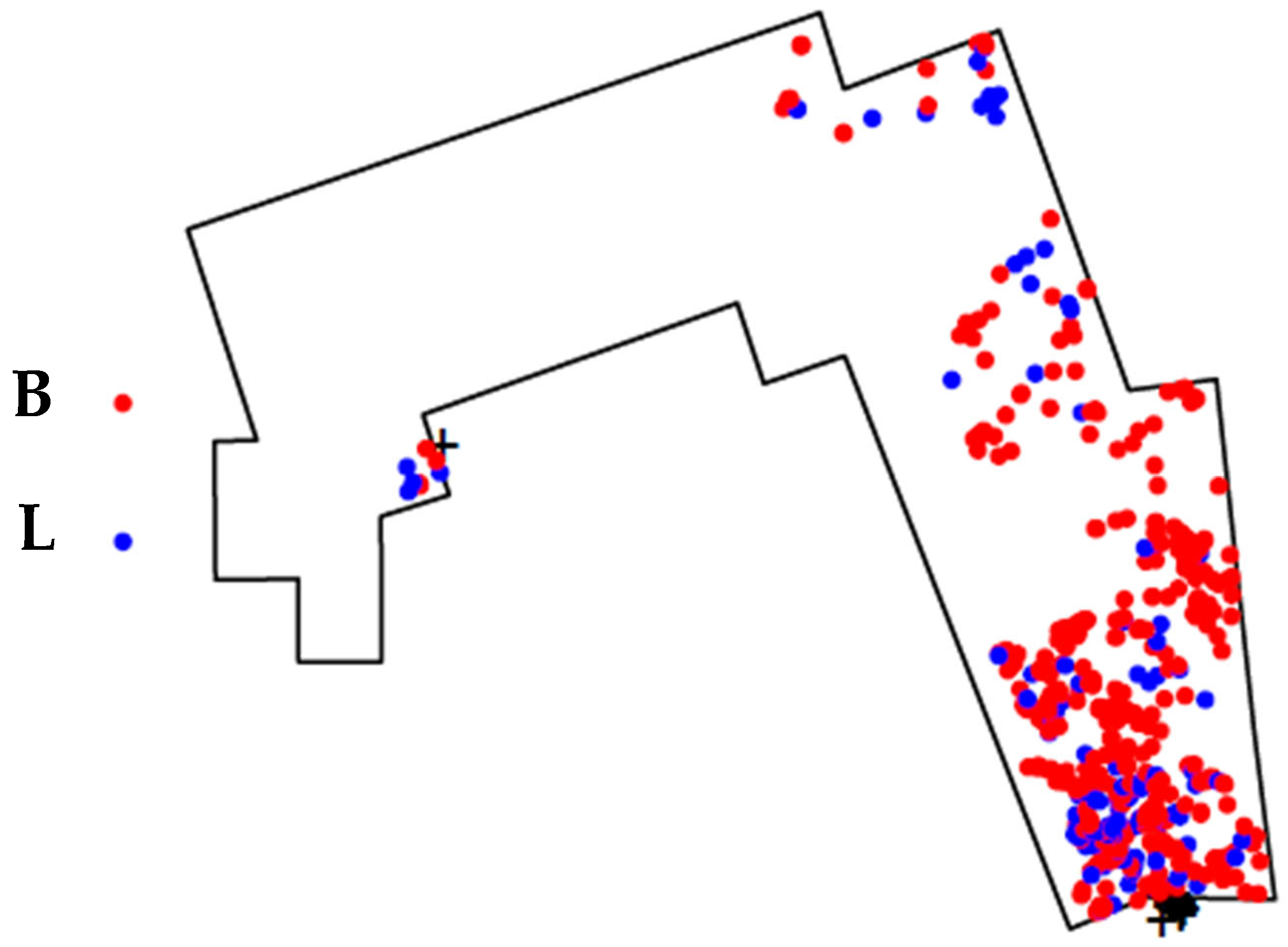In contrast with other sites from this stratigraphic interval (such as FLK Zinj or PTK), level 22A from DS appears to contain a much lower density of remains than level 22B [43]. However, the excavation area was initially defined based on the fossil densities observed in level 22B. The lower concentration of materials towards the south was considered to delineate the site boundaries at that specific level, whereas in the case of level 22A, in this area, the trend was the opposite, indicating a higher density of materials as we approached the 22B level wall (Figure 1). This observation suggests that there may still be materials associated with level 22A to be uncovered [36,43].

Domínguez-Rodrigo et al. [1] underscored the significance of emphasizing not just skeletal part representation but also the physical alteration of bones by biotic and abiotic agents involved in the formation of the assemblage. Therefore, considering this “Physical Attribute Approach”, bone modifications were considered, based on this integrative approach, within a broader analytical framework, also involving the analysis of skeletal profiles as part of the more traditional approach to taphonomic study.

• Skeletal profiles

Bone specimens were grouped following Bunn’s proposed system [19] into small carcasses (sizes 1 and 2), medium-sized carcasses (size 3), and large carcasses (sizes 4, 5, and 6) and divided into cranial (horn, skull, mandible, and loose teeth), axial (ribs, vertebrae, scapulae, and pelves), appendicular (long limb bones), and compact (carpals, tarsals, patella, phalanges, and sesamoids) elements. Long limb bones were further categorized into upper (humerus and femur), intermediate (radius and tibia), and lower (metapodials) limb bones, following the classification outlined by Domínguez-Rodrigo [84].

Bone fragments were also categorized based on their shape (flat, cube, and tube) and composition (dense or trabecular), since it has long been argued that these are factors which play a crucial role in abiotic transportation processes [36,85,86,87,88,89,90,91]. A bone fragment was classified as “flat” if its thickness was less than one-third of its width, “cube” if the thickness was greater than one-third of the width, and “tube” if it was a shaft from a long bone. As for the composition, bones were labeled as “dense” if dense tissue constituted more than two-thirds of the specimen and “trabecular” if the cancellous bone structure made up more than one-third of the bone’s composition [91].

The NISP (number of identifiable specimens) estimates for level 22a considered specific element and animal sizes, but not taxa [19,92,93]. Such remains are, therefore, identifiable to an anatomical element only. As for the case of appendicular elements, they were divided according to the bone portion into proximal ends, mid-shafts, and distal ends. The minimum number of elements (MNE) was determined following a manual overlap specimen approach by systematically arranging all the identified specimens of a specific skeletal element on a large table, grouping them based on the bone portion, and counting the most frequently represented the portion of each particular element, taking into account both the overlapping and non-overlapping bone specimens, as well as carcass size and, when identifiable, side and age [94,95].

Initial MNI (minimum number of individuals) estimates were computed using only the cranial skeleton. However, this approach has the potential to introduce bias in estimating the number of carcasses accumulated by hominins, since teeth are more resistant to post-depositional processes and individuals unrelated to the rest of the assemblage could be considered in the MNI, contributing to a potential overestimation [61,96,97]. Therefore, a second MNI estimate was calculated using only appendicular elements (humeri and tibiae, as they were the most abundant identifiable appendicular elements in the assemblage), offering a more conservative assessment of the minimum number of carcasses comprising the assemblage.

Breakage planes and patterns were measured and analyzed. We identified dry and green fractures, and as per the criteria outlined by Villa and Mahieu [98], we measured the plane angle with respect to the cortical (longitudinal or oblique concerning the long axis) for the latter using a goniometer. We also considered and quantified fracture notches according to type: (1) complete notches (type A); (2) incomplete notches (type B); (3) double overlapping notches (type C); (4) double opposing complete notches (type D); and (5) micro notches (<1 cm) [99,100]. Finally, when possible, limb bones were classified according to the shaft circumference into type 1 (<50% of the original circumference), type 2 (>50%), or type 3 fragments (complete circumference) [19].

Lastly, the preservation and disturbance of the cortical surfaces were also assessed, as well as an examination of bone surface modifications, including cut marks, tooth marks, percussion marks, and diagenetic alterations such as abrasion, trampling, or biochemical marks. Marks were first identified through hand lenses under direct light and documented based on the type of bone element and the specific section where they were observed, if identifiable, following the methodology outlined by Domínguez-Rodrigo [84,101], since this can ease the identification of access patterns by hominins and carnivores.

• Aging Method

For aging the DS ungulate remains, we used Bunn and Pickering’s method [102]. Bunn and Pickering’s age-determination framework for African ungulates draws on the well-established correlation between tooth development and chronological age. In their studies, they applied detailed dental analysis to classify individuals into five initial categories based on eruption and wear stages, which were then collapsed into three broader functional age classes—juvenile, prime adult, and old adult—for mortality profile analysis. For both gazelles and wildebeests, whose dental development is well-documented and progresses in relatively predictable sequences, these assessments focused on the mandibular cheek teeth (premolars and molars), which are preserved well archeologically and exhibit clear ontogenetic and functional wear patterns.

In gazelles, the young juvenile class includes individuals with erupting or recently erupted deciduous premolars and first permanent molars (M1), with minimal to no wear. These animals are typically less than one years old. Subadult juveniles, nearing prime age, show the full eruption of M1 and M2, with attrition on premolars and an emerging M3. Prime adults exhibit fully erupted permanent dentitions (P2–P4 and M1–M3) with moderate wear, reflecting animals in peak physical condition and reproductive maturity, usually between 2 and 5 years of age. Late prime adults are marked by a loss of mesial infundibulum in M1. Old adults display heavy wear, particularly on the M1–M2, with dentine exposure and, in some cases, dental attrition extending into the pulp cavity, which are signs of senescence often seen in animals older than 6–7 years.

In wildebeests, a similar progression applies with different timing, though with age-adjusted thresholds due to their larger size and longer lifespan. Juveniles are identified by the presence of deciduous dentition. Prime adults have fully erupted and moderately worn permanent molars, especially M1 and M2, indicating active foraging and physical peak, often between 3 and 6 years. The old-adult category includes individuals with advanced dental wear, frequently characterized by cupped molars, extensive dentine exposure, and the flattening of cusps, which suggests reduced foraging efficiency and advanced age—generally beyond 8 years. The attribution to old age in this ungulate size was established using the loss of the mesial infundibulum of the first molar as the threshold, which usually correlates with about 60% of the potential life span.

To generate mortality profiles, Bunn and Pickering grouped these dental categories into three broader functional classes: juveniles (young juvenile + subadult juvenile), prime adults (early + late prime), and old adults. These were plotted using triangular graphs to assess population-level mortality patterns. Their analyses showed that carnivore-accumulated assemblages (e.g., hyena dens) tended to produce attritional profiles, rich in juveniles and old individuals, consistent with natural vulnerability. In contrast, the prime-dominated profiles observed at some hominin-associated sites (such as FLK Zinj) pointed to selective acquisition—interpreted as evidence for active hunting rather than opportunistic scavenging. This refined, taxon-specific use of dental aging for gazelles and wildebeests (given the much faster rate of dental attrition in the former) provides a critical foundation for interpreting behavioral patterns in Plio-Pleistocene hominin ecology when using the age profiles of the animals that they consumed.

• The hot–cold zone approach to cut-mark analysis

Domínguez-Rodrigo et al.’s [1] “hot zone/cold zone” framework is a spatially explicit and anatomically grounded method for analyzing the distribution of cut marks on long bones in archeological and experimental assemblages. This approach was developed to address limitations in earlier cut-mark studies that either treated long bones as uniform surfaces or relied solely on frequency counts, which could obscure the functional and behavioral interpretations of butchery. The core idea is that certain anatomical areas of long bones are more likely to exhibit cut marks during defleshing or disarticulation, depending on their muscular load, connective tissue density, and butchery accessibility, according to whether access to the carcass is primary (through bulk defleshing) or secondary (through kleptoparasitism).

Hot zones are anatomical regions on long bones where cut marks are most likely to occur during systematic butchery, especially for meat removal during bulk defleshing. They are referred to as “hot” because they are indicative of access, since they correspond to zones where flesh-eating carnivores (namely, felids) do not leave flesh scraps after their primary access to carcasses. Cut marks on such locations are most likely to be inflicted by hominins during bulk defleshing, and therefore, primary access to carcasses. In contrast, cold zones correspond to muscle insertions, ligament attachments, and articular margins, which require slicing through during carcass processing, regardless of access type. These areas also display flesh scraps more commonly after flesh-eating carnivores intervene, primarily in carcass consumption. Cut marks located on these sections, therefore, could be ambiguously indicative of hominin primary access (imparting marks during dismembering or regular defleshing) or their secondary intervention to exploit available flesh scraps abandoned by other carnivores. Their location is thus ambiguous regarding butchery action and access type.

In the methodology, long bones (e.g., humerus, femur, tibia) are divided into standardized anatomical quadrants and segments using clear skeletal landmarks. Each bone is mapped three-dimensionally along its longitudinal axis (proximal to distal) and circumferentially (anterior, posterior, medial, lateral). The distribution of cut marks is then documented across these defined zones. Domínguez-Rodrigo et al. [1] validated this method using controlled butchery experiments with modern carcasses, systematically documenting the location and frequency of cut marks during defleshing, dismemberment, and skinning and the observation of flesh scrap availability on carcasses initially consumed by felids.

B.

AI Analysis of the DS22a BSMs

• Sample

In order to ensure the identification of the agents and processes involved in the formation of DS level 22A, we conducted an AI-driven analysis of the BSMs identified on the faunal remains, consisting of 35 marks, which were compared to experimental BSMs created under controlled conditions, including cut marks, tooth marks, and trampling marks. Given the size of the assemblage, and the variety of processes observed and overlapping, this approach was deemed the most efficient and objective to assess agency in this part of the study.

Regarding the experimental tooth-mark collection, we utilized part of the experimental assemblage reported in Abellán et al. [71] and Domínguez-Rodrigo et al. [52]. This sample comprises 1169 tooth pits and scores associated with three carnivores: leopards (n = 543), lions (n = 263), and hyenas (n = 363). In the first stage of the analysis, we implemented a lion–hyena model because these species are the primary extant carnivores frequently identified as potential interactors with hominins in Pleistocene contexts. Additionally, the carcass damage documented does not show any evidence of crocodile activity, such as bisected tooth marks, and most marks were identified in size 3 carcasses, outside of the preferred weight range of leopards [103,104,105,106]. We also later implemented a leopard–hyena model to ensure a more objective classification, as we identified five marks on two size 1 elements. For detailed information on the experimental carnivore-generated sample, refer to Cobo-Sánchez et al. [39] and Domínguez-Rodrigo et al. [52].

In the Early Pleistocene, Crocuta crocuta was absent, but its ancestral forms, Crocuta ultra and the earlier Crocuta dietrichi, were present [107]. In the case of Olduvai Bed I, hyena dental remains exhibit metrics, particularly p3 and p4, that fall within the variation range of modern Crocuta crocuta [108] and, therefore, as we assume minimal variation may exist between the tooth-mark morphologies of the modern and prehistoric hyenas, should such variation exist, we posit that extinct hyenas tooth marks would be more similar to the ones created by modern hyenas than any other carnivore.

Tooth marks made by lions and leopards are less problematic, as both Panthera leo and Panthera pardus have a well-established record that goes back to about 2 Mya or even further [107]. Therefore, lion and leopard tooth marks from Bed I would likely be very similar, if not identical, to those made by modern specimens.

The cut and trampling marks’ referential collection was the one reported by Pizarro-Monzo et al. [80], consisting of 150 cut marks and 154 trampling grooves documented. We used this more recent collection instead of the earlier cut-mark–trampling collection [69] because the latter displayed lower image quality and reported low recall for trampling marks [74].

Both the BSMs identified in the DS assemblage and the carnivore referential marks were photographed in a standardized way using the same Leica Emspira 3 digital microscope at 30× magnification. In the case of the experimental sample, we magnified exceedingly small marks to ×50 to ensure the clear visualization of shape and morphology details, although these variations were standardized during the preprocessing of images before analysis [43,78]. Cut marks and trampling marks in the referential collection were captured using an Olympus LEXT OLS3000 Confocal Laser Microscope and a KH-8700 3D Digital Microscope with high-intensity LED optics and 30x magnification [67]. The code and images are available at https://doi.org/10.7910/DVN/A5F4SN and https://doi.org/10.7910/DVN/BQTKBA.

• Methods and Models

Given the success achieved in previous AI-based taphonomic analyses, we have relied again on models based on transfer learning (TL), utilizing pretrained architectures and models previously trained on vast datasets in order to enhance their capacity to discern microscopic features in BSMs. TL helps mitigate overfitting by reducing the number of trainable parameters and enhancing performance on small datasets.

Analysis of tooth marks through DL.

In the case of tooth marks, we used three deep learning models: DenseNet 201, ResNet 50, and VGG19 [109,110,111,112], which had been successfully used before for the analysis of DS 22B [63] and other assemblages. These individual models were complemented with ensemble learning (EL) techniques for comparison. Our preprocessing and implementation DL methodology follows that outlined in Cobo-Sánchez et al. [39] and Domínguez-Rodrigo et al. [38] for the tooth-mark sample. First, for the DL analysis of the BSM, the dataset was divided into training (75%) and testing (25%) sets, with randomized assignment to avoid biases. The training set utilized mini-batch cores of size 64, while testing employed cores of size 32, with weight updates performed over 100 epochs—100 times—with 100 steps each through backpropagation. We standardized our sample after resizing the images to 250 × 200 pixels, then applied data augmentation techniques, including rotation, shifting, horizontal flipping, and normalization, as well as a testing of Dropout rates varying from 0.3 to 0.8 in order to reduce the possibility of overfitting that can result from using a training dataset that is too small and without enough data to effectively capture the full range of potential input data values—in this case, BSMs. To preserve the learned features from the pretrained model, all layers of DenseNet 201, ResNet 50, and VGG19 are set as non-trainable, ensuring that their weights remain unchanged during training. A custom classification head is then added on top of the feature extractor. First, a Flatten layer converts the extracted feature maps into a one-dimensional vector. This is followed by a fully connected (dense) layer with 128 neurons, ReLU activation, and He uniform initialization, which help stabilize training by properly scaling the weight initialization. A Dropout layer (30%) is included to reduce overfitting by randomly deactivating neurons during training. The final layer is a single neuron with a sigmoid activation function, suitable for binary classification tasks, as it outputs a probability score between 0 and 1.

The model is compiled with the stochastic gradient descent (SGD) optimizer, using a learning rate of 0.001 and a momentum of 0.9, which helps accelerate training while avoiding local minima. The binary cross-entropy loss function is used, as it is appropriate for binary classification, and accuracy is set as the evaluation metric. This configuration makes the model well-suited for binary image classification tasks while leveraging the feature extraction capabilities of the models.

This description of the DL-TL models is pertinent to explain the derived models that we used for the classification of the DS tooth marks; however, these architectures were used and borrowed from Cobo-Sánchez et al. [39]. As indicated before, the code and images are accessible through the original publication.

Analysis of cut–trampling marks through Few-Shot Learning (FSL).

For the analysis of cut–trampling marks, we employed a meta-learning approach denominated Model-Agnostic Meta-Learning (MAML). MAML is one of the algorithms used in few-shot learning (FSL). In this scenario, the advantage of MAML versus DL is that it is adaptable to learning quickly with limited training data [113], as is the case with our experimental cut and trampling sample. The selected base architectures also included ResNet 50 and DenseNet 201 alongside ResNet152, a more advanced framework that employs advanced computational strategies to optimize classification performance. The MAML model was built on the output feature maps from the last convolutional layer of each base model, with additional layers added for better feature representation and classification. The initial MAML layers included two residual blocks with depthwise separable convolutions (kernel size = 3, stride = 1, padding = “same”), enabling hierarchical feature learning essential for few-shot learning. These depthwise separable convolutions reduced computational costs by decomposing standard convolutions into spatial and depthwise operations, reducing the trainable parameters.

FSL models require the precise calibration of shot–task configurations to optimize performance. In this context, “shot” refers to the number of labeled samples per class, while “task” denotes a single classification episode involving distinct data subsets. Achieving an optimal balance between shots and tasks is challenging, as different proportions yield varying levels of model performance. To assess the most effective configuration, we evaluated two scenarios: a) Low-shot scenario: characterized by a limited number of labeled samples per class but a greater number of classification tasks; b) High-shot scenario: featuring a higher number of labeled samples per class but fewer overall tasks. Striking the right balance between shot and task numbers is critical in FSL. Excessive shots can lead to overfitting, diminishing the model’s capacity for generalization. Conversely, an excessive number of tasks with insufficient shots may hinder effective feature learning. Empirical research suggests that prioritizing tasks over shots generally enhances generalization, though the optimal balance remains task-dependent.

The present study aimed to determine the most effective shot–task ratio for BSM classification within a meta-learning framework. Here, in all our experimental modeling, the low-shot technique achieved better results. Therefore, we implemented a 5–20 shot–task ratio.

For the MAML analysis of the cut–trampling marks, image standardization was conducted using bidimensional matrices for centering and normalization, applying preprocessing functions specific to each deep learning architecture. All images were resized to match the original dimensions utilized in the transfer learning (TL) models. Consequently, images were adjusted to 224 × 224 pixels for the ResNet and DenseNet architectures. Given that most tooth marks exhibit a high degree of visual similarity to the human observer, this high-resolution approach was designed to enhance the deep learning process by enabling finer differentiation among classificatory features. The dataset was partitioned into training (70%), validation (15%), and testing (15%) subsets. Data augmentation and regularization protocols were the same as described for the DL models above. To mitigate overfitting, we employed multiple regularization techniques, including Dropout, Batch Normalization (BN), Early Stopping, and Learning Rate Scheduling. Dropout rates ranging from 0.3 to 0.8 were tested, but performance variations remained minimal, likely due to its interaction with BN, which stabilized learning by normalizing feature distributions. BN further counteracted potential Dropout-induced drawbacks by scaling and shifting feature distributions, ensuring stable training dynamics. Early Stopping was implemented by monitoring the validation loss, halting training if no improvement occurred after 15 epochs, and restoring the model to its best-performing weights. Additionally, Learning Rate Scheduling was applied, progressively reducing the learning rate by a factor of 0.1 at predefined epochs to facilitate smoother convergence.

Each model was implemented using two different activation functions and two optimizers. The activation function plays a key role at the start of the learning process, helping the model identify potential patterns in the data. The optimizer, on the other hand, fine-tunes this learning by adjusting parameters based on the learning rate, which controls the step size the model takes when improving, and the momentum, which helps maintain and smooth the learning. Therefore, we compared two activation functions (“ReLU” and “Swish”) and two optimizers (stochastic gradient descent (SGD) and Adagrad), using a learning rate of 0.001 and a momentum of 0.9, and selected the best combination to ensure the best performance (for details, see Supplementary Information).

To assess performance and evaluate the classification results, we relied on accuracy, F1 scores—a useful metric for measuring performance when you have imbalanced data because it takes into account false positives and false negatives—and training and loss graphs. Marks were considered agent-specific only when both models agreed in the attribution and at least one of them produced classification probabilities greater than 80%. Marks for which one of the models provided a different agent classification were discarded, as they would not be considered reliable. All computation processes were carried out at the Institute of Evolution in Africa (IDEA) through a GPU HP Z6 Workstation using a CUDA (cuDNN) environment and Python version 3.7.

3. Results

A.

Taphonomic study

• Taxonomic and skeletal profiles

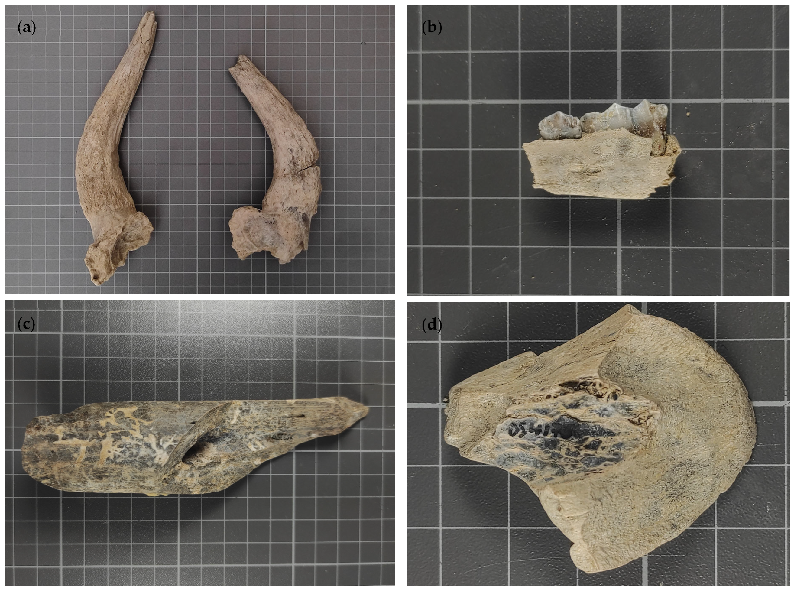
In contrast to the substantial number of elements recovered from level 22B [37], only 136 macro-faunal remains, excluding those of a few small carnivores (viverrids), birds and testudines, are associated with level 22A of the DS site. Despite the small sample size, it encompasses an intriguing variety of specimens (Figure 2), predominantly bovids, but also includes remains of megafauna (hippopotamus and elephant) and even an exceptionally well-preserved hyoid bone from a size 3 individual.

Out of 136 remains, 45 (33% of the sample) are from small carcasses, 82 from medium-sized carcasses (60%), 5 from big animals (4%), and only 4 remains (3%) could not be assigned to a carcass size. As for the skeletal profile analysis, it reveals a minimum number of eleven individuals (MNI), comprising seven small individuals (sizes 1–2), including one suid, three medium-sized animals (sizes 3–4), and one large carcass (size 5–6) based on cranial MNI (

Table 1. Minimum number of individuals (MNI) represented by teeth (stratified by age) and by postcranial elements.

	MNI Cranial				MNI Postcranial
	Taxa	Subadult	Prime	Old	Subadult	Adult
Size 1–2	Antidorcas recki	1	3	2		2
	Kolpochoerus heseloni	1
Size 3–4	Equus sp.		1			3
	Kobus sigmoidalis			1
	Parmularius altidens		1
Size 5–6	Hippopotamus sp.		1			2
	Elephas sp.

). When examining solely the limb bones, however, and particularly the humeri and tibiae, which are the most represented appendicular elements, the MNI indicates two small carcasses, three medium-sized carcasses, and two large carcasses, including remains identifiable as belonging to Elephas sp.

When comparing the MNI to the MNE (

Table 2. Minimum number of elements (MNE) documented at level 22A from DS.

MNE
Carcasses	Small-Sized	Medium-Sized	Large-Sized
Horn	2
Cranium		2
Teeth	4	5	1
Mandible	6	1
Hyoid		1
Vertebrae	2	3	1
Pelvis	2	3	1
Scapula	2	2
Ribs	3	3	1
Humerus	2	3	1
Radius–ulna	2	2
Metacarpal	1	2	1
Femur	2	2
Tibia–fibula	2	3	3
Metatarsal	2	1
Carpal/tarsal		1
Phalanges	1	4	1

), we see how many skeletal parts are present for each carcass size: long bones are the most representative elements of the assemblage, with a high survival of cortical mid-shafts, while significant representation also comes from teeth and mandibles across all size classes, suggesting the robust preservation of denser skeletal parts, whereas the proportion of epiphysis is low, possibly related to fragmentation associated with human or carnivore activity [100,114,115], as well as the proportion of indeterminate elements.

Table 3. Minimum number of specimens (NISP) documented at level 22A from DS.

NISP
Carcasses		Small-Sized	Medium-Sized	Large-Sized
Horn		2
Skull			5
Teeth		4	5	1
Mandible		8	2
Hyoid			1
Vertebrae
	cervical	2
	thoracic		1
	lumbar			1
	other		3
Pelvis		3	6	1
Scapula		2	3
Ribs		3	3	1
Humerus
	proximal end
	mid-shaft	3	7	1
	distal end		2
Radius–ulna
	proximal end	1	1
	mid-shaft	3	4
	distal end
Carpals
Metacarpal
	proximal end		2	1
	mid-shaft	2	3
	distal end	1		1
Femur
	proximal end		2
	mid-shaft	2	3
	distal end		1
Tibia–fibula
	proximal end
	mid-shaft	4	2	5
	distal end	1	2
Tarsals			1
Metatarsal
	proximal end		1
	mid-shaft	2
	distal end	1
Phalanges		1	5	1
Others			1
ULB				4
ILB
LLB			1

shows the skeletal part representation according to the number of identifiable specimens (NISP).

The collection is mostly composed of prime adult carcasses, with a tendency towards younger individuals in the case of small animals and a limited representation of large-sized animals. The predominance of prime adult carcasses may indicate active selection by hominins, since prime adults offer the highest return in terms of meat and fat, making them the most valuable targets [102,116].

• Bone breakage

A total of 92 (68%) elements exhibit either green breakage, dry breakage, or both. Out of these remains, 36 exhibit exclusively green fractures (39.1%), 40 exhibit only dry fractures (43.5%), and 16 exhibit both types (17.4%). Another 17 elements bear fractures that were not assigned to dry or green due to their ambiguity. This similar proportion of green and dry fractures suggests multi-stage taphonomic processes, including perimortem activities and later post-depositional disturbances due to static loading. The majority of the green breakage (26 out of 36 [72.2%]) can be found on appendicular bones with multiple fragments refitting, indicating on-site processing [1,82,117], but also on axial, specifically on pelvis, and cranial remains (five each [13.9%]). As for dry fractures, they are documented mostly on axial (18 [45%]) and appendicular remains (17, [43%]), and marginally on cranial (2 [0.5%]); the remaining three are associated with indeterminate fragments.

Shaft circumferences can also give valuable information about bone breaking processes [19]. Type I is the predominant type of long bone fragment (36 out of 62 long bones = 58%), followed by type III (n = 19 [30%]) and type II (n = 7 [11%]). This predominance of type I shafts also suggests extensive breakage, often associated with intensive processing activities, such as marrow extraction by hominins using hammerstones or significant gnawing by carnivores.

A total of 13 notches were identified in the assemblage. The most common type is micronotches (n = 4), followed by types A (n = 3), B, C, and D (n = 2 for each type). Most notches are located on long bones, particularly tibiae (n = 4), but they are also present on a femur, radius, humerus, and metacarpus. Additionally, two micronotches are found on a mandible and a pelvis. Micronotches, the most frequent type, are typically associated with subtle loading forces, such as light percussion activities or carnivore gnawing [99,100,118,119].

Several of the long bones exhibiting notches (specifically, two tibiae, the femur, the humerus, and the metacarpus) also display percussion pits and cut marks, while one element (radius) shows potential carnivore scores. The predominance of notches on long bones, along with these associated marks, aligns with the structural suitability of these elements for marrow retention and the shared interest of both hominins and carnivores in processing these elements for nutritional purposes [99].

• Bone surface modifications

The cortical surfaces of the assemblage are generally very well-preserved, with no evidence of weathering (except for an element that displays stage 2 weathering; the rest of the assemblage (99.92%) shows no subaerial modifications). There is also no evidence of polishing or abrasion indicative of water disturbance, suggesting that DS represents an autochthonous deposit that was quickly buried in a stable environment after deposition (S2). Only two specimens exhibit signs of polishing or abrasion, likely resulting from geological processes or biomechanical forces over time [56]. This excellent overall preservation has facilitated the identification of potential human and carnivore marks and other alterations attributed to biotic agents, such as biochemical alterations, which were subsequently documented and analyzed using neural networks.

A total of 11 skeletal elements exhibit evidence of carnivore tooth marks or gnawing. These modifications are most frequently observed in size 3–4 individuals (n = 6), while four altered elements correspond to size 1–2 animals, and a single size 5 pelvis shows signs of alteration. The majority of these modifications are found on long bones, specifically on intermediate and lower limbs (n = 6 [54.5%]); however, carnivore damage is also present on two pelves, a vertebra, and a mandible.

Additionally, 19 skeletal elements bear possible cut marks, most of them located on long bones (n = 12). Among these, upper limb bones (ULBs) and intermediate limb bones (ILBs) are the most commonly affected (n = 11). Nearly all cut-marked elements (n = 18) belong to size 3–4 animals, with only one specimen from a size 1–2 individual; this corresponds to 27.3% of the medium-sized animals of the NISP bearing cut marks and 2% of the small-sized animals’ NISP (Table 3). Of these appendicular elements with cut marks, six also exhibit percussion pits, indicating marrow extraction. Additionally, two of these elements refit. When applicable, the exact anatomical location of the cut marks was recorded using the hot-zone approach (see [1]). Six long bones exhibited cut marks within hot zones—muscle-rich areas typically targeted during defleshing. Tibiae were the most frequently modified elements, with cut marks consistently distributed along the mid-shaft and lower diaphysis and present on all anatomical faces: cranial, caudal, medial, and lateral. One femur displayed cut marks on the cranial aspect, specifically at the transition between the distal diaphysis and metaphysis, an area within the hot zone associated with major muscle attachment and detachment. Similarly, two scrape marks were observed on the cranial face of a humerus, located near the teres tuberosity, further indicating intensive defleshing. In a radius, a cut mark was identified on the medial aspect, near the proximal epiphysis, but still within the defined hot-zone range. Lastly, one metacarpal exhibited cut marks along the cranial face of the mid-shaft (for details, see S1).

The high percentage of cut-marked long bone specimens located primarily in “hot zones”—areas where little flesh remains following consumption by lions—strongly suggests that hominins had primary access to the carcasses, consuming the meat and later extracting bone marrow. Further evidence of hominin involvement is provided by the presence of cut marks on axial bones, including two ribs, a scapula, and a pelvis, which supports the hypothesis that hominins had primary access to bulk flesh from entire carcasses and utilized them extensively. Moreover, the presence of cut marks on a mandibular condyle and a phalanx suggests that hominins may have also engaged in disarticulation and skinning activities, indicating a comprehensive butchery process.

B.

AI analysis

The presence of bone surface modifications (BSMs) made by humans and/or carnivores, combined with the good preservation of the remains and minimal evidence of weathering, abrasion, or erosion, provides important insights into the taphonomic history of the site, making this a highly informative assemblage for interpreting past human and carnivore interactions.

In total, 35 marks—20 possible cuts and 15 scores—were selected and documented through a binocular microscope and compared to cut marks, tooth marks, and trampling marks obtained in controlled conditions in order to ensure the identification of the agents involved in the creation of the assemblage.

Most of the marks were documented on size 3 individuals, but five modifications were identified on two size 1 remains, which is the reason why we first implemented a lion–hyena model and later a leopard–hyena one for those marks associated with small individuals.

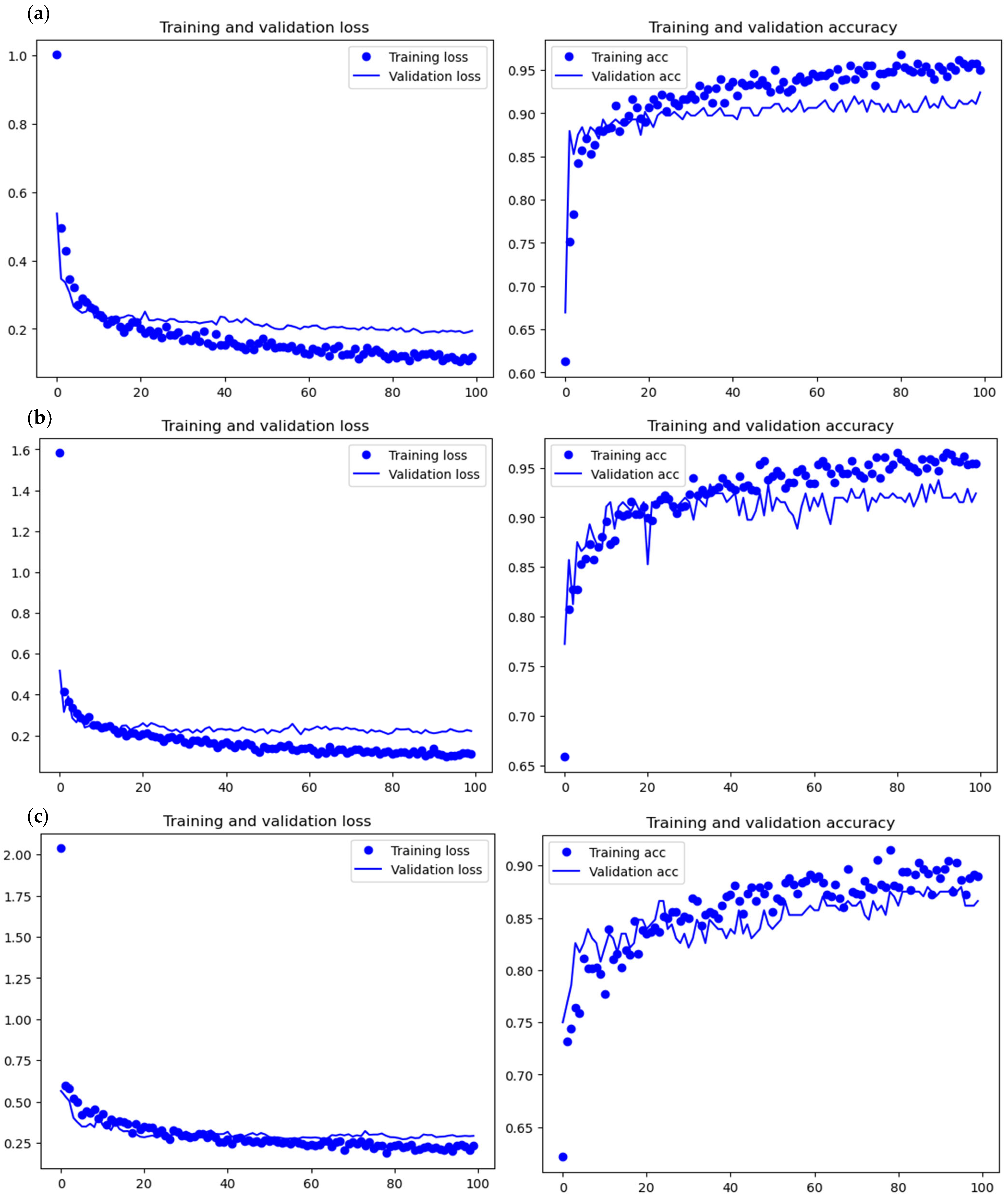
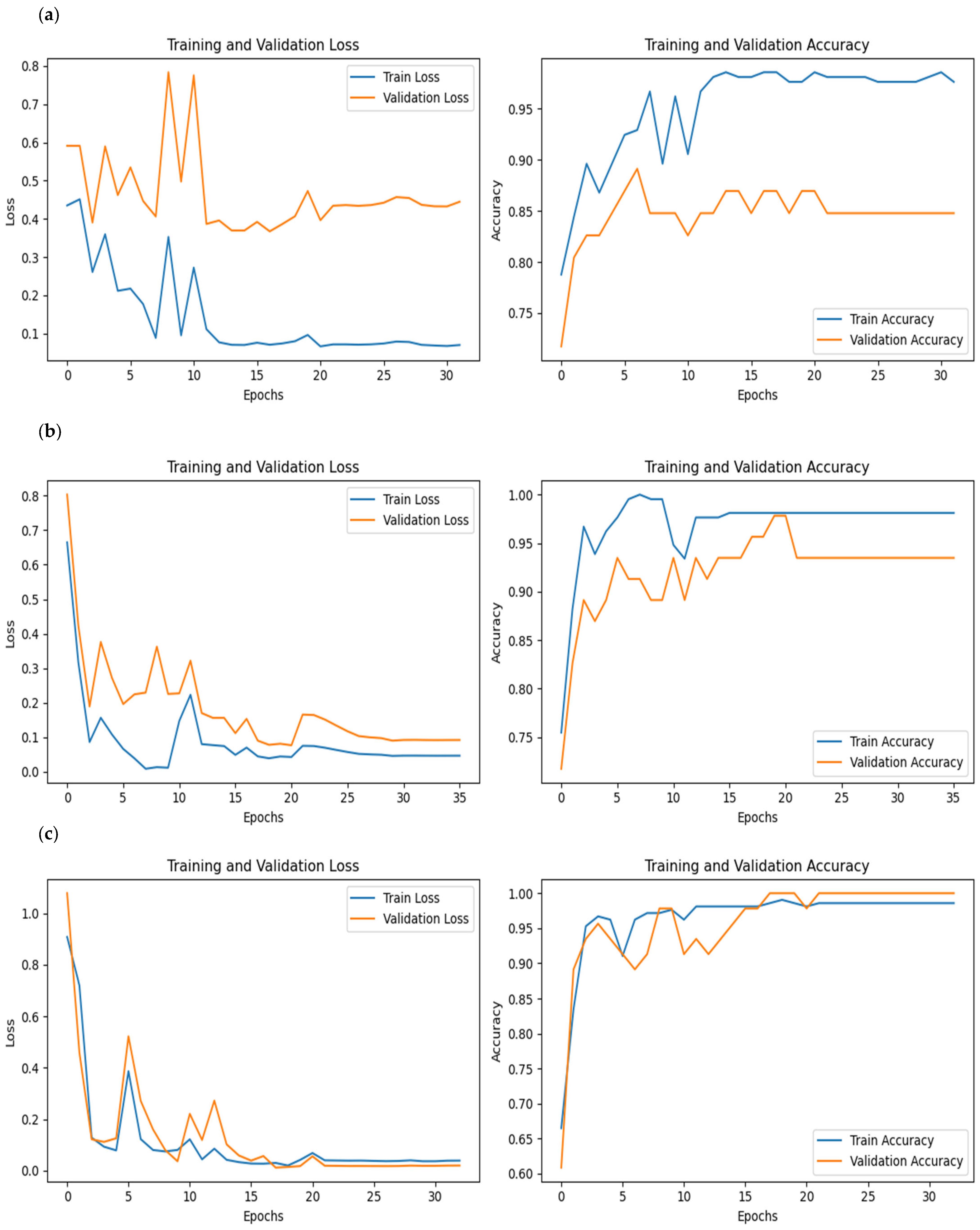
All of the implemented architectures displayed a regular training process with all BSMs clearly differentiated and classified in the early stages of the analysis (Figure 3 and Figure 4). Overfitting was not an issue, since the accuracy of the training set is not substantially different from that of the validation set, and the shape of both during the training process is similar. This is also supported by the loss values. Overfitting should be inferred if loss values for the training set are low, but high in the validation/testing, which does not occur in this case.

For the lion–hyena scenario, the models yielded unambiguous classifications of the BSMs. In total, 12 out of 15 marks were classified as tooth marks made by hyena with 99% confidence (

Table 4. Probability of classification for each tooth mark according to agent for the lion–hyena model.

Sigla	Mark Number	Densenet 201		Resnet50		Vgg19		Ensemble Decision
		lions	hyenas	lions	hyenas	lions	hyenas	lions	hyenas
DS 4616	DS1	0.93	0.07	0.0241	0.975	0.821	0.179	-	x
	DS2	0.001	0.999	4.32 × 10−5	0.999	4.32 × 10−6	0.999	-	x
	DS3	0.0001	0.999	1.09 × 10−7	0.999	7.88 × 10−6	0.999	-	x
	DS4	0.0081	0.991	0.00023	0.999	7.44 × 10−5	0.999	-	x
	DS5	0.0002	0.999	1.30 × 10−7	0.999	2.80 × 10−5	0.999	-	x
	DS6	0.018	0.982	1.00 × 10−4	0.999	6.00 × 10−3	0.994	-	x
	DS7	0.001	0.999	1.08 × 10−5	0.999	6.05 × 10−6	0.999	-	x
DS 4628	DS8	0.418	0.582	4.00 × 10−3	0.996	2.00 × 10−3	0.998	-	x
DS 2777	DS9	0.004	0.996	7.00 × 10−4	0.999	4.16 × 10−1	0.584	-	x
DS 3336	DS10	0.06	0.94	1.20 × 10−2	0.988	4.60 × 10−1	0.54	-	x
	DS11	0.09	0.91	1.40 × 10−2	0.986	7.30 × 10−2	0.927	-	x
	DS12	0.0007	0.999	5.00 × 10−4	0.999	1.28 × 10−1	0.872	-	x
DS 3320	DS13	0.81	0.19	1.22 × 10−1	0.878	9.90 × 10−1	0.01	-	x
	DS14	0.325	0.675	2.10 × 10−2	0.979	9.90 × 10−1	0.01	-	x
DS 3387	DS15	0.0001	0.999	3.66 × 10−8	0.999	1.00 × 10−4	0.999	-	x

). The leopard–hyena models implemented for the marks associated with size 1 remains did not show a resolution as high as the lion–hyena ones but also tended towards hyenas (

Table 5. Probability of classification for each tooth mark according to agent for the leopard–hyena model.

Sigla	Mark Number	Densenet 201		Resnet50		Vgg19		Ensemble Decision
		leopards	hyenas	leopards	hyenas	leopards	hyenas	leopards	hyenas
DS 3336	DS10	0.1382	0.86	0.1438	0.85	0.495	0.51	-	x
	DS11	0.1574	0.84	0.1227	0.87	0.1391	0.86	-	x
	DS12	0.0174	0.98	0.1149	0.88	0.3797	0.62	-	x
DS 3320	DS13	0.4264	0.57	0.2505	0.75	0.6998	0.30	-	x
	DS14	0.5184	0.48	0.1494	0.85	0.3275	0.67	-	x

). The ensemble decision in both cases was hyena for all the marks.

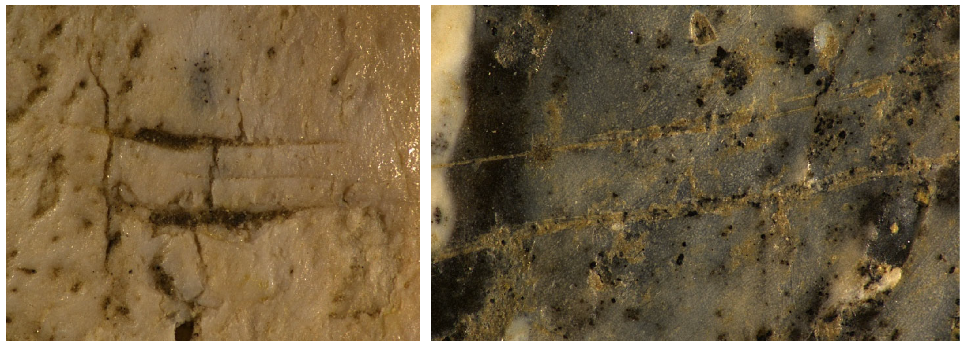
In total, 20 marks were identified as cut marks with accuracies over 97% (

Table 6. Probability of classification for each possible cut mark.

Sigla	Mark Number	Cut-Mark Probability	Trampling Mark Prob.	Ensemble Decision
DS 4389	DSC1	0.976	0.024	CM	TMP
	DSC2	0.976	0.024	x	-
DS 4628	DSC3	0.976	0.024	x	-
DS 4226B	DSC4	0.976	0.024	x	-
DS 4423	DSC5	0.976	0.024	x	-
	DSC6	0.976	0.024	x	-
	DSC7	0.976	0.024	x	-
DS 4183	DSC8	0.976	0.024	x	-
	DSC9	0.976	0.024	x	-
	DSC10	0.976	0.024	x	-
DS 4175	DSC11	0.976	0.024	x	-
	DSC12	0.976	0.024	x	-
	DSC13	0.976	0.024	x	-
	DSC14	0.976	0.024	x	-
DS 4626	DSC15	0.976	0.024	x	-
	DSC16	0.976	0.024	x	-
	DSC17	0.976	0.024	x	-
	DSC18	0.976	0.024	x	-
	DSC19	0.976	0.024	x	-
DS 3350	DSC20	0.976	0.024	x	-

). These cut marks were identified mainly on hot zones from long bone specimens but also on mandibular remains, axial bones, and phalanges (Figure 5). This suggests that hominins had primary access to bulk flesh from whole carcasses, intensively exploiting and skinning them before they were later scavenged by hyenas.

Considering the dense vegetation surrounding the DS site in this 1.8 myo context [120], hominins likely utilized an ambush strategy to capture small to medium-sized carcasses.

4. Discussion

The faunal assemblage from level 22A of DS (Bed I, Olduvai Gorge) provides significant insights into early hominin behaviors, site formation processes, and ecological interactions in the Plio-Pleistocene landscape. Despite the relatively small sample size, the assemblage’s exceptional preservation enables a detailed taphonomic study that bridges traditional analyses with innovative AI-based methodologies.

From a classical taphonomic perspective, the skeletal representation, dominated by cranial and mid-shaft appendicular elements, the suggests selective preservation of dense bones, influenced by both hominin and carnivore activity as confirmed later by the AI analysis [27,114]. The high representation of cut marks on long bones, traditionally used as proxies for identifying primary access and intensive carcass processing, and mandibular fragments indicates that hominins had primary access to bulk flesh, supporting the hypothesis of systematic butchery practices even in Early Pleistocene contexts [9,84]. More significantly, over half of the appendicular elements exhibit cut marks within anatomically defined “hot zones”—areas typically devoid of flesh following primary carnivore consumption, such as by felids. This spatial distribution of cut marks, especially along mid-shafts and muscle-rich portions of the tibiae, femur, humerus, and radius, points toward primary access to meat, systematic defleshing, and complete butchery sequences carried out by hominins [1].

In contrast, tooth marks, primarily attributed to hyenids, reflect subsequent scavenging. The anatomical distribution of these marks suggests that carnivores predominantly targeted grease-rich regions, such as epiphyseal ends and cancellous bone. This sequential pattern of carcass use, with hominins as likely primary agents and carnivores as secondary scavengers, underscores the dynamic nature of predator–prey interactions in the paleoecological context of Olduvai Gorge.

The dual occurrence of green and dry fractures indicates both perimortem and post-depositional processes. The limited occurrence of polishing and abrasion suggests sporadic movement, possibly driven by localized sediment reworking or biomechanical forces rather than prolonged fluvial transport or trampling. Moreover, the absence of significant weathering or water disturbance underscores the site’s autochthonous nature and rapid burial in a stable environment.

Age class distribution data adds yet another layer of behavioral inference. The prevalence of prime adult individuals among the medium-sized carcasses aligns with a pattern of selective acquisition typical of hunting behavior [121,122]. This pattern diverges from the attritional profiles generally produced by carnivore accumulation, which tend to favor vulnerable juveniles and old adults [121,122]. This strengthens the case for deliberate carcass selection and transport by hominins.

On the other hand, deep learning models and convolutional neural networks (CNNs) excel in pattern recognition and have demonstrated high precision in distinguishing carnivore-induced modifications [66,70,71,72], percussion marks and cut marks, even discriminating between flesh and defleshed carcasses or tool materials [68,123]. By automating the classification process, DL minimizes human subjectivity and enhances reproducibility, a crucial advancement for refining taphonomic interpretations. Moreover, the implementation of meta-learning techniques, such as Model-Agnostic Meta-Learning (MAML), further improves adaptability by enabling models to quickly adjust to new datasets with minimal retraining [113]. This is particularly beneficial in taphonomy, where site-specific variability in bone surface preservation can pose challenges to static classification models. The integration of AI methodologies into this study, therefore, enhances interpretations and addresses the longstanding issues of equifinality and subjectivity in BSM analysis. The successful implementation of transfer learning and few-shot learning algorithms allowed for a robust classification of bone surface modifications, even within a relatively small dataset. The models achieved high confidence levels (often >97% for cut marks and >99% for hyena tooth marks), supporting the reliability of the observed patterns. Moreover, ensemble decision-making across multiple model architectures further mitigated individual model biases, enhancing the overall robustness of agent attribution.

In sum, the DS 22A assemblage stands out not only for its preservation and complexity but also for its demonstration of how classical and modern methodologies can be synergistically combined. By aligning cut-mark location and frequency, tooth-mark classification, age profiles, and AI-based BSM attribution, this study provides not just confirmation of anthropogenic agency but a complete behavioral narrative: carcasses were acquired in relatively complete condition, defleshed intensively in meat-bearing areas, disarticulated, and, in many cases, broken open for marrow extraction—before being abandoned and later scavenged. Despite these advancements, challenges remain in fully integrating AI into taphonomic research. One primary limitation is the need for extensive annotated datasets to train models effectively. While experimental and actualistic studies contribute to these datasets, variability in archeological contexts must be taken into account, since post-depositional processes can alter bone surface modifications, modifying certain features that may not be fully accounted for in experimental samples [77]. This can introduce biases and create difficulties in identifying patterns in archeological contexts. Future research should focus on expanding training datasets with diverse BSM examples and refining ML architectures to account for site-specific post-depositional processes.

5. Conclusions

The DS 22A assemblage provides crucial evidence of early hominin behavioral complexity, ecological interactions, and site formation processes. Although still in a preliminary stage, the taphonomic analysis reveals a complex interplay between hominin and carnivore activities, offering early insights into the adaptive flexibility of hominins in resource exploitation within a competitive ecological framework.

Traditional variables such as cut-mark frequency and distribution, green bone fractures, and skeletal part representation strongly support the interpretation of systematic butchery and marrow extraction by hominins, consistent with primary access to carcasses. The spatial and anatomical distribution of cut marks, particularly in muscle-rich ‘hot zones’, further reinforces the notion of deliberate defleshing activities. Complementary evidence from carnivore modifications, dominated by hyenid tooth marks on grease-rich elements, indicates a secondary scavenging behavior, highlighting the ecological interplay between hominins and carnivores at the site. This sequential use underscores the interspecies competition characteristic of Plio-Pleistocene ecosystems.

The minimal weathering, erosion, and abrasion demonstrate the rapid burial of the assemblages in a stable depositional environment, preserving surface modifications with remarkable clarity and suggesting level 22a as an autochthonous deposit. This exceptional preservation and limited diagenetic alteration underscore the importance of sedimentary contexts in maintaining taphonomic integrity.

Finally, the integration of deep learning and meta-learning techniques into taphonomic analysis yielded significant accuracy and provides a more robust support for the interpretations of biotic and anthropogenic interactions in multipatterned scenarios. This methodological innovation sets a precedent for future studies, particularly in assemblages where traditional analyses are constrained by surface degradation or analyst subjectivity.

This study underscores the value of integrating traditional taphonomic approaches with AI-based techniques to refine our understanding of early hominin lifeways. The DS 22A assemblage, with its excellent preservation and rich taphonomic signatures, offers a critical window into the behavioral and ecological dynamics of early hominin populations in the Olduvai Gorge. By leveraging AI, taphonomic research can move beyond traditional limitations, incorporating large-scale datasets and advanced computational techniques to refine our understanding of past dynamics.

Ultimately, the ongoing advancement and application of AI in archeology will offer deeper insights into hominin subsistence strategies, site formation processes, and the broader paleoecological landscape. Meanwhile, in the near term, efforts should prioritize expanding annotated datasets, enhancing model interpretability, and refining hybrid approaches that integrate AI with taphonomic expertise. This will enable a more objective and standardized classification of BSMs, ensuring consistency in data interpretation, facilitating the replication of analyses, and mitigating research biases.