Statistical Modeling for Nanofluid Flow: A Stretching Sheet with Thermophysical Property Data

Abstract

This paper reports the use of a numerical solution of nanofluid flow. The boundary layer flow over a stretching sheet in combination of two nanofluids models is studied. The partial differential equation that governs this model was transformed into a nonlinear ordinary differential equation by using similarity variables, and the numerical results were obtained by applying the shooting technique. Copper (Cu) nanoparticles (water-based fluid) were used in this study. This paper presents and discusses all numerical results, including those for the local Sherwood number and the local Nusselt number. Additionally, the effects of the nanoparticle volume fraction, Brownian motion Nb, and thermophoresis Nt on the performance of heat transfer are discussed. The results show that the stretching sheet has a unique solution: as the nanoparticle volume fraction φ (φ = 0), Nt (Nt = 0.1), and Nb decrease, the rate of heat transfer increases. Furthermore, as φ (φ = 0) and Nb decrease, the rate of mass transfer increases. The data of the Nusselt and Sherwood numbers were tested using different statistical distributions, and it is found that both datasets fit the Weibull distribution for different values of Nt and rotating φ.

1. Introduction

In recent years, many researchers have investigated stretching plates, which are used in industry for materials such as lubricants and glass fibers. The theory of flow over a stretching plate was first proposed by Crane [1]. Researchers [2] have also analyzed heat transfer over a stretching sheet with a permeable surface. Related studies involving a stretching surface were conducted by Grubka and Bobba [3], Ali [4], Wang [5], and Hayat et al. [6]. Convective heat transfer is a very important property of nanofluids, and the addition of nanoparticles has been found to improve the thermal conductivity. Widely used types of nanoparticles include monotubes, carbide nanoparticles, and metal nanoparticles, which can be added to base fluids such as glycol, ethylene, and engine oil. One of the important properties of nanofluids is their ability to enhance the thermal properties of fluids. Nanofluids have numerous applications, including electronics, biomedicine, nuclear reactors, and space technology. Khan [7], Choi [8], Masuda [9], Choi [10], and Wang [11] used nanoparticles to study the thermal conductivity. In the presence of nanoparticles, Wang [12] examined heat transfer and nanofluid flow by using a nanofluid model, which can also be used to study hydromagnetic flow over a permeable sheet [13]. Using a nanofluid model, Bachok [14] studied the effect of two elements in nanofluids, namely, Brownian motion and thermophoresis. These elements have been used to characterize the flow over a permeable surface [15] and an isothermal vertical plate [16]. Flow and heat transfer in turbulent flow were studied by Z. Taghizabeh-Tabari [17], and their results showed that the rate of heat transfer enhancement and pressure drop increment were greater for a plate heat exchanger (PHE) under turbulent flow conditions. Mahian [18] asserted that it is crucial to use measured data for thermophysical properties to predict the heat transfer coefficient with high accuracy. The analysis reported in [19] revealed that the effect of adding nanoparticles to the base fluid has a strong influence on the heat transfer enhancement by increasing the Reynolds number of flows and increasing the heat transfer. Heydari [20] used water as the base fluid and investigated the effect of the volume fraction of nanoparticles (TiO₂) on the heat transfer and physical properties of the fluid. In a different approach, Hemmat [21] introduced and used a neural network as a powerful tool for estimating the thermophysical properties of nanofluids. The resulting empirical relationship could predict the thermal conductivity coefficient of water–EG–Al₂O₃ nanofluid with acceptable precision. Pourfattah [22] numerically investigated the rate of heat transfer enhancement for the flow regime inside a tube. The rotating flow in fluids has also been studied extensively in the past several years. The rotating flow over a stretching sheet is significant in several manufacturing processes, such as the extrusion of plastic sheets, glass blowing, fiber spinning, and continuous molding [23]. Usoicz [24] studied a physical–statistical model that provided highly accurate predictions of the thermal conductivity of nanofluids. Because nanofluids are essential in many applications, understanding their fundamental properties is crucial for exploring their use and potential benefits. Previous studies have demonstrated that the effective enhancement of the base fluid is important for improving its thermal efficiency [25]. Therefore, in this paper, building on previous studies [26,27], we propose combining the two nanofluid equation models developed by Buongiorno [15] and Tiwari and Das [12]. Our objective is to determine the effect of two key parameters: thermophoresis and Brownian motion. The shooting technique was used to obtain the results for the local Sherwood number and local Nusselt number. We present a physical–statistical model, as well as its distribution to predict the thermal conductivity of a fluid containing copper nanoparticles. The proposed model can be used for a wide range of practical applications in further studies on nanofluids.

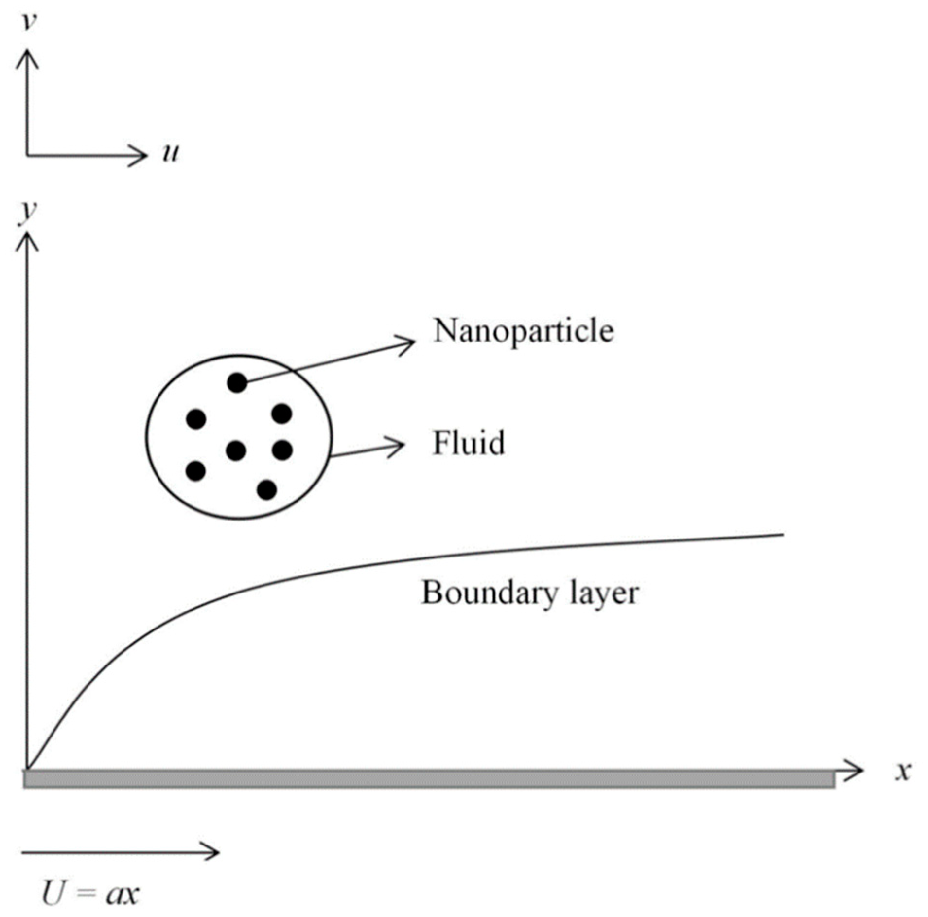
2. Problem Formulation

We consider the three-dimensional free convection boundary layer flow for an area $y>0$ past a stretching sheet, with a stagnation point $x=0$ and conditions for the plane $y=0$. We consider the flow to be incompressible, laminar, and steady. The flow is assumed to have a stretching velocity $U_W\left(x\right)$ that varies linearly from $x=0$, with $U_W\left(x\right)=ax$ and $U_{\infty }\left(x\right)=bx$ ($a, b$ are constants, with $b>0$). The scheme of the physical configuration is depicted in Figure 1.

The same assumption also applies to the velocity of the fluid $U_{\infty }\left(x\right)$. The governing equations for a stretching sheet, where $a>b$, are as follows.

$$\frac{\partial u}{\partial x}+\frac{\partial v}{\partial y}=0$$

(1)

$$u\frac{\partial u}{\partial x}+v\frac{\partial u}{\partial y}=U_{\infty }\left(x\right)\frac{d{U}_{\infty }}{dx}+\frac{{\mu }_{nf}}{{\rho }_{nf}}\frac{{\partial }^2\mu }{\partial y^2}$$

(2)

$$u\frac{\partial T}{\partial x}+v\frac{\partial T}{\partial y}= {\alpha }_{nf}\frac{{\partial }^{2}T}{\partial y^2}+\tau \left[D_B\frac{\partial C}{\partial y}\frac{\partial T}{\partial y}+\left(\frac{D_T}{T_{\infty }}\right){\left(\frac{\partial T}{\partial y}\right)}^2\right]$$

(3)

$$u\frac{\partial C}{\partial x}+v\frac{\partial C}{\partial y}=D_B\frac{{\partial }^{2}C}{\partial y^2}+\left(\frac{D_T}{T_{\infty }}\right)\frac{{\partial }^{2}T}{\partial y^2}$$

(4)

subject to

$$u=U_w\left(x\right), v=0, T=T_w, C=C_w\mathrm{at}y=0$$

(5)

$$u\to U_{\infty }, T\to T_{\infty }, C\to C_{\infty },\mathrm{as} y\to \infty$$

where v is the velocity of the component in the y-direction, and u is the velocity of the component in the x-direction. T_w, T_∞, and T are the surface temperature, ambient temperature, and temperature, respectively. C is the nanoparticle volume fraction, C_∞ is the nanoparticle volume fraction far from the plate, and C_w is the nanoparticle volume fraction at the plate. D_T is the coefficient of thermophoretic diffusion, and D_B is the coefficient of Brownian diffusion. The ratio of heat capacity is τ = (ρC_p)_s/(ρC_p)_f, in which (ρC_p)_s represents the heat capacity of the nanoparticle, and (ρC_p)_f represents the heat capacity of the fluid. Further, α_nf is the nanofluid thermal diffusivity, μ_nf is the nanofluid viscosity, and ρ_nf is the nanofluid density. These parameters were previously described by Oztop [28].

$${\alpha }_{nf}=\frac{k_{nf}}{{\left(\rho C_p\right)}_{nf}}, {\rho }_{nf}=\left(1-\phi \right){\rho }_f+\phi {\rho }_s, {\mu }_{nf}=\frac{{\mu }_f}{{\left(1-\phi \right)}^{2.5}}$$

(6)

$${\left(\rho C_p\right)}_{nf}=\left(1-\phi \right){\left(\rho C_p\right)}_f+\phi {\left(\rho C_p\right)}_s, \frac{k_{nf}}{k_f}=\frac{\left(k_s+2k_s\right)-2\phi \left(k_f-k_s\right)}{\left(k_s+2k_s\right)+\phi \left(k_f-k_s\right)}$$

(7)

where the parameter φ is the nanoparticle volume fraction, (ρC_p)_nf is the heat capacity of the nanofluid, k_nf is the thermal conductivity of the nanofluid, k_f is the thermal conductivity of the fluid, k_s is the thermal conductivity of the solid, ρ_f is the fluid density, μ_f is the fluid viscosity, and ρ_s is the density of the solid. According to Abu-Nada [25], the term k_nf is used for spherical nanoparticles, and its value is negligible for other shapes. Next, given the constraints in Equation (5), the similarity solution of Equations (1)–(4) is computed; Equation (4) was proposed by Buongiorno [15]. We introduce the similarity transformations below.

$$\eta ={\left(\frac{U_{\infty }}{v_{f}x}\right)}^{\frac{1}{2}}y, \psi ={\left({\upsilon }_{f}x{U}_{\infty }\right)}^{\frac{1}{2}}f\left(\eta \right), \theta \left(\eta \right)=\frac{T-T_{\infty }}{T_w-T_{\infty }}, \varphi \left(\eta \right)=\frac{C-C_{\infty }}{C-C_{\infty }}$$

(8)

where $\theta \left(\eta \right)$ is a dimensionless variable for temperature, and $\varphi \left(\eta \right)$ is a dimensionless variable for nanoparticle concentration. The boundary conditions are

$$u=U_w\left(x\right), v=0, T=T_w,C=C_w at y=0$$

$$u\to U_{\infty },T\to T_{\infty },C\to C_{\infty } as y\to \infty ,$$

$$\frac{1}{{\left(1-\phi \right)}^{2.5}\left(1-\phi +\phi {\rho }_s/{\rho }_f\right)}{f}^{‴}+f{f}^{’’}-f^{’2}+1=0$$

(9)

$$\frac{1}{Pr}\frac{k_{nf}/k_f}{\left(1-\phi +\phi {\left(\rho C_p\right)}_s/{\left(\rho C_p\right)}_f\right)}{\theta }^{″}+\frac{1}{2}f{\theta }^{\prime }+Nb{\varphi }^{\prime }{\theta }^{\prime }+Nt{\theta }^{’2}=0$$

(10)

$${\varphi }^{″}+\frac{1}{2}Lef{\theta }^{\prime }+\frac{Nt}{Nb}{\theta }^{″}=0,$$

(11)

subject to the boundary conditions

$$\begin{gathered} f\left(0\right)=0,f^{\prime }\left(0\right)=\epsilon ,\theta \left(0\right)=1,\varphi \left(0\right)=1, \\ {f}^{\prime }\left(\eta \right)\to 1,\theta \left(\eta \right)\to 0, \varphi \left(\eta \right)\to 0 as \eta \to \infty \end{gathered}$$

(12)

The Brownian motion parameter is

$$Nb=\frac{{\left(\rho c\right)}_p{D}_B\left(C_w-C_{\infty }\right)}{{\left(\rho c\right)}_f\nu },$$

the thermophoresis parameter is

$$Nt=\frac{{\left(\rho c\right)}_p{D}_T\left(T_w-T_{\infty }\right)}{{\left(\rho c\right)}_f{T}_{\infty }\nu },$$

the Prandtl number is

$$Pr=\frac{\nu }{\alpha },$$

the Lewis number is

$$Pr=\frac{\nu }{D_B},$$

the stretching parameter is

$$\epsilon = a/b,$$

the skin friction coefficient is

$$C_{f}R{e}_x^{1/2}=\frac{1}{{\left(1-\phi \right)}^{2.5}}{f}^{″}\left(0\right),$$

the local Nusselt number is

$$N{u}_{x}R{e}_x^{-1/2}=-\frac{k_{nf}}{k_f}{\theta }^{\prime }\left(0\right),$$

the local Sherwood number is

$$S{h}_{x}R{e}_x^{-1/2}=-{\varphi }^{\prime }\left(0\right),$$

and the local Reynolds number is

$$R{e}_x=Ux/v_f.$$

The data for the Nusselt and Sherwood numbers were tested using the Akaike information criterion (AIC). This test is used to find the goodness of fit and determine the distribution that best fits the data.

Table 1. The distribution test for Nusselt and Sherwood numbers.

Distribution	Cumulative Distribution Function, F(x)
Lognormal	$F\left(x\right)=\frac{1}{2}+\frac{1}{2}erf\left[\frac{ln\left(x\right)-\mu }{\sigma \sqrt{2}}\right]$
	where erf is the complete error function;$\sigma$ is the shape of the distribution; x is the value used to evaluate the function;$\mu$ is the expected value for the normal distribution.
Weibull	$F\left(x\right)=1-exp\left[{\left(-\frac{x}{\alpha }\right)}^{\beta }\right]$
	where x is the value used to evaluate the function;$\alpha$ is the scale parameter;$\beta$ is the shape parameter.
Rayleigh	$F\left(x\right)=1-exp\left[\left(-\frac{x^2}{2{\sigma }^2}\right)\right]$
	where x is the value used to evaluate the function;$\sigma$ is the shape of the distribution.
Exponential	$F\left(x\right)=1-exp\left(-\frac{x}{\theta }\right)$
	where x is the value used to evaluate the function;$\theta$ is the scale parameter.
Gamma	$F\left(x\right)=\frac{\gamma \left(\alpha ,\frac{x}{\beta }\right)}{\Gamma \left(\alpha \right)}$
	where $\Gamma \left(\alpha \right)$ is the incomplete gamma function; x is the value used to evaluate the function;$\alpha$ is the shape parameter;$\beta$ is the scale parameter.
Inverse Gaussian	$F\left(x\right)=\Phi \left[\sqrt{\frac{\lambda }{x}}\left(\frac{x}{\mu }-1\right)\right]+e^{\frac{2\lambda }{\mu }}\Phi \left[-\sqrt{\frac{\lambda }{x}}\left(\frac{x}{\mu }+1\right)\right]$
	where x is the value used to evaluate the function; $\Phi$ denotes the distribution function of the standard normal; $\mu$ is the mean;$\lambda$ is the shape parameter.
Inverse Gamma	$F\left(x\right)=\frac{\gamma \left(p,\frac{\beta }{x}\right)}{\Gamma \left(p\right)}$
	where $\Gamma \left(p\right)$ is the incomplete gamma function; x is the value used to evaluate the function;$\alpha$ is the shape parameter;$\beta$ is the scale parameter.

lists the different statistical distributions. For each distribution in the table, the AIC was calculated, and the best distribution was identified from the AIC values.

The AIC measures the quality of statistical models for a sample set of data. The model that provides the lowest AIC value best fits the data. The formula for the AIC is

$$AIC=-2\log \left(L\right)+2k$$

where L is a model of the likelihood function, and k is the number of parameters.

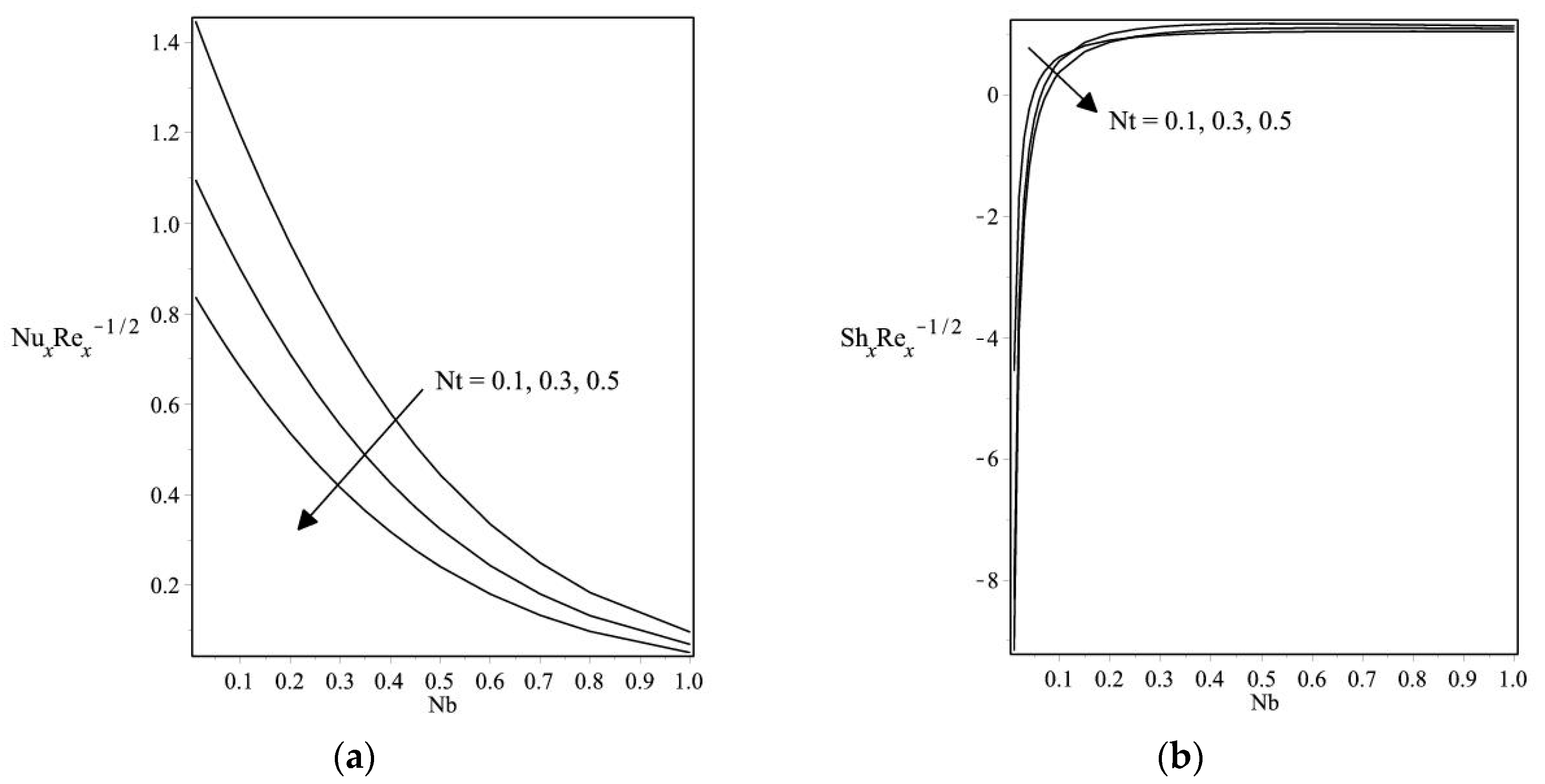
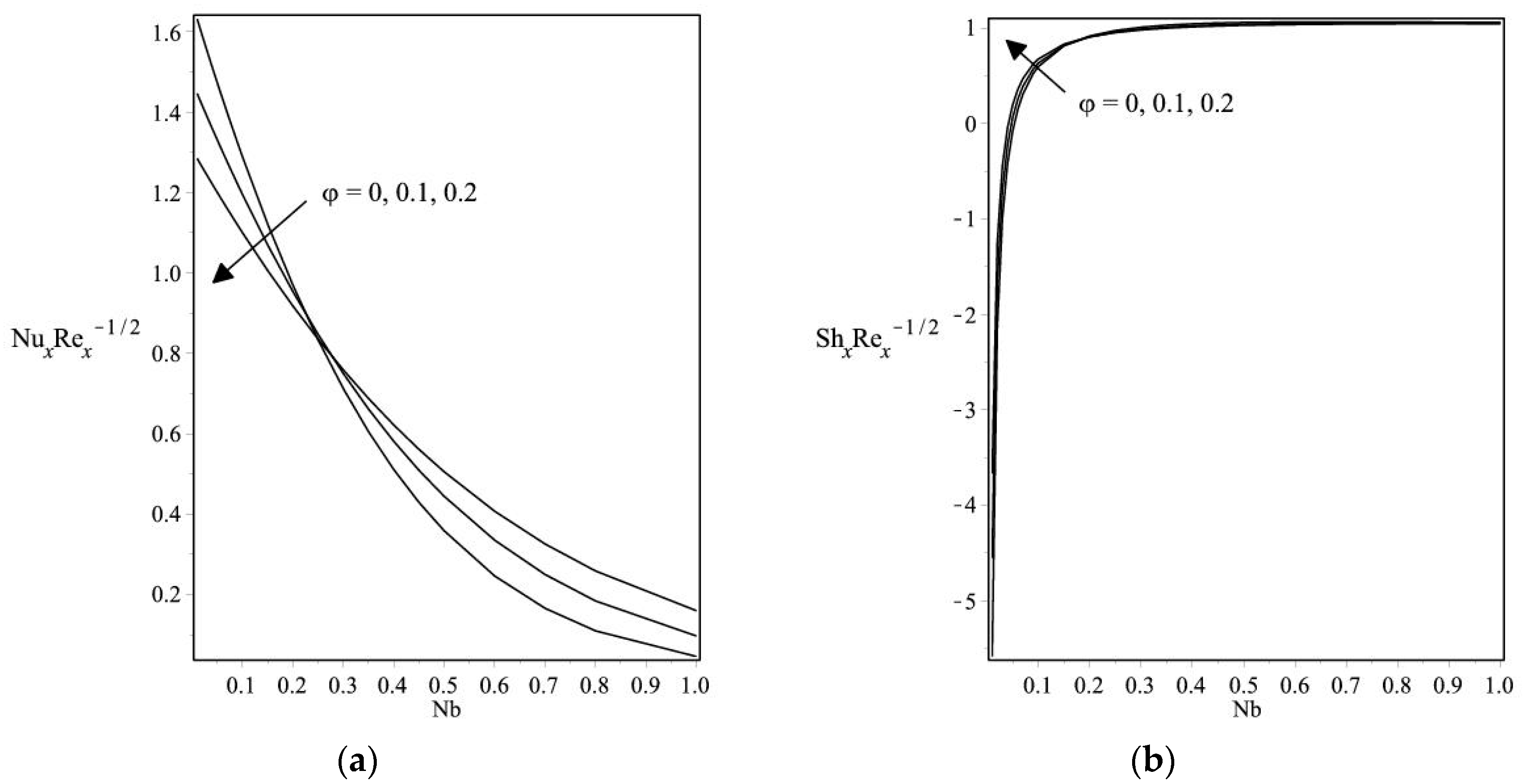
3. Results and Discussion

The shooting technique was used to determine the numerical solutions for Equations (9)–(11) with the boundary conditions in Equation (12). The shooting method converts a boundary value problem (BVP) into an initial value problem (IVP). The main reason for using the shooting method is that it can establish the applicable initial conditions for a related IVP to generate the solution to the BVP. This method was applied in the Maple programming language using the “dsolve” command and “shoot” implementation. The influences of Nb, Nt, and φ on the heat transfer rate were investigated for Cu nanoparticles. The values of the thermophysical properties are shown in

Table 2. Thermophysical properties of a nanofluid [18].

Physical Properties	Base Fluid	Nanoparticle, Cu
	Water
Cp(J/kgK)	4179	385
ρ (kg/m3)	997.1	8933
k (W/mk)	0.613	400

.

When φ = 0 for a regular fluid, the range of φ should be 0–0.2 [18]. The value of Pr (Prandtl number) is 6.2. Figure 2a,b depicts the variation in the local Nusselt number and Sherwood number with Nb for different Nt when φ = 0.1, Pr = 6.2, Le = 3, and ε = 1.2 for the stretching case. As clearly shown in Figure 2a, as Nb increases, the local Nusselt number decreases, while Figure 2b shows the opposite trend. Furthermore, Figure 3a,b shows that the local Nusselt number and local Sherwood number vary with Nb for different φ when Pr = 6.2, Nt = 0.1, Le = 3, and ε = 1.2 for the stretching case. These figures reveal that as Nb increases, the local Nusselt number and local Sherwood number decrease. It is important to note that the Brownian motion parameter Nb and thermophoresis Nt are related to the random motion of nanoparticles (Cu). For small values of Nb and Nt, the viscosity of the base fluid is weak, and the nanoparticles (Cu) tend to move easily among each other. Because of this phenomenon, the fluid is cooled faster, and the heat transfer rate increases.

On the basis of Figure 2 and Figure 3, the data for the Nusselt and Sherwood numbers were further analyzed to obtain the statistical properties for the tested distributions.

Table 3. Parameters of statistical distributions for the Nusselt number.

		Nusselt
		Nt			φ
		0.1	0.3	0.5	0	0.5	1
Weibull	alpha	1.114028	0.880117	0.707426	1.147663	1.114028	1.060899
	beta	2.071876	2.044809	2.03204	2.042564	2.071873	2.107767
Lognormal	u	0.597253	−0.4527	−0.6728	−0.1882	−0.2134	−0.257
	sigma	0.205756	0.5687	0.5733	0.5735	0.5581	0.5406
Exponential	ʘ	5.958346	0.784728	0.63081	1.023495	0.993058	0.945277
Rayleigh	ʘ	0.783248	0.620077	0.498912	0.808725	0.783248	0.743932
Gamma	alpha	2.576506	2.532032	2.512095	2.518703	2.576506	2.645924
	beta	2.594448	3.226632	3.9823	2.460647	2.594448	2.799164
InvGaussian	u	0.996058	0.784728	0.63081	1.023495	0.993058	0.945277
	lambda	0.585994	0.458409	0.366933	0.594599	0.585994	0.567803
InvGamma	p	1.128832	1.465284	1.840917	1.141713	1.128832	1.130869
	beta	1.561164	1.537004	1.528137	1.520823	1.561164	1.609246

and

Table 4. Parameters of statistical distributions for the Sherwood number.

		Sherwood
		Nt			φ
		0.1	0.3	0.5	0	0.5	1
Weibull	alpha	0.8744 11	0.898522	0.817144	0.979489	0.874401	0.797106
	beta	2.577703	3.371081	1.81384	3.554751	2.577703	2.790235
Lognormal	u	−0.4244	−0.3095	−0.6076	−0.2249	−0.4244	−0.499
	sigma	0.6062	0.2281	1.1546	0.2703	0.6062	0.5926
Exponential	ʘ	0.789122	0.805275	0.74553	0.883678	0.789712	0.723538
Rayleigh	ʘ	1.328239	3.12215	4.058364	1.278631	1.328239	1.389953
Gamma	alpha	2.809859	5.54345	1.741032	5.098837	2.809859	3.006884
	beta	3.55806	6.883961	2.335395	5.769994	3.55806	4.156075
InvGaussian	u	0.789712	0.805275	0.74553	0.883678	0.789712	0.723538
	lambda	0.585994	0.690534	0.210486	0.707045	0.419399	0.380038
InvGamma	p	2.10314	0.406664	7.750569	0.502391	2.10314	2.441288
	beta	1.176628	3.838668	0.628842	2.976252	1.176628	1.121279

show the parameters for different distributions that were tested with the data.

Table 5. Akaike information criteria (AIC) for the Nusselt number.

		Nusselt
		Nt			φ
		0.1	0.3	0.5	0	0.5	1
Weibull	AIC	28.0644	19.87677	12.15149	29.47854	28.0644	25.89071
Lognormal	AIC	489.2136	32.11579	24.22703	41.67786	40.65745	38.98349
Exponential	AIC	72.25254	29.27293	21.41297	38.83604	37.7492	35.97403
Rayleigh	AIC	28.09332	19.88825	12.15742	29.4889	28.09332	25.95421
Gamma	AIC	130.558	155.573	181.8519	121.6317	130.558	143.5579
InvGaussian	AIC	43.14529	34.74409	26.90818	44.40187	43.14529	41.17968
InvGamma	AIC	66.38085	61.39603	59.74171	64.92191	66.38085	68.1083

and

Table 6. Akaike information criteria (AIC) for the Sherwood number.

		Sherwood
		Nt			φ
		0.1	0.3	0.5	0	0.5	1
Weibull	AIC	12.54905	5.472407	13.72022	8.515101	12.54905	8.096197
Lognormal	AIC	26.92753	33.11634	23.53942	38.58843	26.92753	23.25246
Exponential	AIC	23.38957	19.23543	17.53949	26.53744	23.38957	19.58635
Rayleigh	AIC	35.5429	59.7277	77.45971	29.54075	35.5429	36.12442
Gamma	AIC	146.2801	361.4002	51.51091	377.5105	146.2801	164.1227
InvGaussian	AIC	29.30123	20.50199	29.48493	28.73508	31.16536	27.70555
InvGamma	AIC	40.39328	131.3749	210.1284	119.6908	40.39328	38.24802

show the Akaike information criteria for the Nusselt and Sherwood numbers. The results show that the lowest AIC values are those for the Weibull distribution. It was also found that as the values of Nt and φ increase, the AIC values still indicate that the Weibull distribution is optimal.

4. Conclusions

Nanofluid flow past a stretching sheet and the influences of parameters Nb, Nt, and φ were examined and studied. From this investigation, a unique solution was obtained for the stretching sheet. It was found that as Nb and Nt decrease, the rate of heat transfer increases, but the rate of mass transfer decreases. The case is different when φ decreases: Nb decreases, and the rates of heat and mass transfer decrease. These results show that for different Nt and φ, the Weibull distribution best fits both the Nusselt and Sherwood data.

References

1. Crane, L.J. Flow past a stretching plate. Z. Angew. Math. Phys. 1970, 21, 645–647. [Google Scholar] [CrossRef]
2. Gupta, P.S.; Gupta, A.S. Heat and mass transfer of a continuous stretching surface with suction or blowing. Can. J. Chem. Eng. 1977, 55, 74–76. [Google Scholar] [CrossRef]
3. Grubka, L.G.; Bobba, K.M. Heat transfer characteristics of a continuous stretching surface with variable temperature. ASME J. Heat Transfer 1985, 107, 248–250. [Google Scholar] [CrossRef]
4. Ali, M.E. Heat transfer characteristics of a continuous stretching surface. Warme Stoffubertragung 1994, 29, 227–234. [Google Scholar] [CrossRef]
5. Wang, C.Y. Analysis of viscous flow due to a stretching sheet with surface slip and suction. Nonlinear Anal. Real World Appl. 2009, 10, 375–380. [Google Scholar] [CrossRef]
6. Hayat, T.; Javed, T.; Abbas, Z. Slip flow and heat transfer of a second grade fluid past a stretching sheet through a porous space. Int. J. Heat Mass Transfer 2008, 51, 4528–4534. [Google Scholar] [CrossRef]
7. Khan, W.A.; Pop, I. Boundary layer flow of a nanofluid past a stretching sheet. Int. J. Heat Mass Transfer 2010, 53, 2477–2483. [Google Scholar] [CrossRef]
8. Choi, S.U.S. Enhancing thermal conductivity of fluid with nanoparticles. In Proceedings of the ASME International Mechanical Engineering Congress and Exposition, San Francisco, CA, USA, 12–17 November 1995; pp. 99–105. [Google Scholar]
9. Masuda, H.; Ebata, A.; Teramae, K.; Hishinuma, N. Alteration of thermal conductivity and viscosity of liquid by dispers- ing ultra-fine particles. Netsu Bussei 1993, 7, 227–233. [Google Scholar] [CrossRef]
10. Choi, S.U.S.; Zhang, Z.G.; Yu, W.; Lockwood, F.E.; Grulke, E.A. Anomalous thermal conductivity enhancement in nanotube suspensions. Appl. Phys. Lett. 2001, 79, 2252–2254. [Google Scholar] [CrossRef]
11. Wang, X.-Q.; Mumjudar, A.S. Heat transfer characteristics of nanofluids: A review. Int. J. Therm. Sci. 2007, 46, 1–19. [Google Scholar] [CrossRef]
12. Tiwari, R.K.; Das, M.K. Heat transfer augmentation in a two-sided lid-driven differentially heated square cavity utilizing nanofluids. Int. J. Heat Mass Transfer 2007, 50, 2002–2018. [Google Scholar] [CrossRef]
13. Kameswaran, P.K.; Narayana, M.; Sibanda, P.; Murthy, P.V.S.N. Hydromagnetic nanofluid flow due to a stretching or shrinking sheet with viscous dissipation and chemical reaction effects. Int. J. Heat Mass Transfer 2012, 55, 7587–7595. [Google Scholar] [CrossRef]
14. Bachok, N.; Ishak, A.; Pop, I. Stagnation-point flow over a stretching/shrinking sheet in a nanofluid. Nanoscale Res. Lett. 2011, 6, 623–633. [Google Scholar] [CrossRef] [PubMed] [Green Version]
15. Boungiorno, J. Convective transport in nanofluids. ASME J. Heat Transfer 2006, 128, 240–250. [Google Scholar] [CrossRef]
16. Bachok, N.; Ishak, A.; Pop, I. Boundary layer stagnation-point flow toward a stretching/shrinking sheet in a nanofluid. J. Heat Transfer 2013, 135, 054501. [Google Scholar] [CrossRef] [Green Version]
17. Taghizadeh-Tabari, Z.; Heris, S.Z.; Moradi, M.; Kahani, M. The study on application of TiO2/water nanofluid in plate heat exchanger of milk pasteurization industries. Renew. Sustain. Energy Rev. 2016, 58, 1318–1326. [Google Scholar] [CrossRef]
18. Mahian, O.; Kianifar, A.; Heris, S.Z.; Wongwises, S. Natural convection of silica nanofluids in square and triangular enclosures: Theoretical and experimental study. Int. J. Heat Mass Transfer 2016, 99, 792–804. [Google Scholar] [CrossRef]
19. Rezaei, O.; Akbari, O.A.; Marzban, A.; Toghraie, D.; Pourfattah, F.; Mashayekhi, R. The numerical investigation of heat transfer and pressure drop of turbulent flow in a triangular microchannel. Phys. E Low-Dimens. Syst. Nanostruct. 2017, 93, 179–189. [Google Scholar] [CrossRef]
20. Heydari, M.; Toghraie, D.; Akbari, O.A. The effect of semi-attached and offset mid-truncated ribs and Water/TiO2 nanofluid on flow and heat transfer properties in a triangular microchannel. Therm. Sci. Eng. Prog. 2017, 2, 140–150. [Google Scholar] [CrossRef]
21. Hemmat, M.E.; Ahangar, M.R.H.; Toghraie, D.; Hajmohammad, M.H.; Rostamian, H.; Tourang, H. Designing artificial neural network on thermal conductivity of Al2O3–water–EG (60–40 %) nanofluid using experimental data. J. Therm. Anal. Calorim. 2016, 126, 837. [Google Scholar] [CrossRef]
22. Pourfattah, F.; Motamedian, M.; Sheikhzadeh, G.; Toghraie, D.; Akbari, O.A. The numerical investigation of angle of attack of inclined rectangular rib on the turbulent heat transfer of Water-Al2O3 nanofluid in a tube. Int. J. Mech. Sci. 2017, 131–132, 1106–1116. [Google Scholar] [CrossRef]
23. Bakar, N.A.A.; Bachok, N.; Arifin, N.M. Rotating Flow Over a Shrinking Sheet in Nanofluid Using Buongiorno Model and Thermophysical Properties of Nanoliquids. J. Nanofluids 2017, 6, 1–12. [Google Scholar] [CrossRef]
24. Usowicz, B.; Usowicz, J.B.; Usowicz, L.B. Physical-Statistical Model of Thermal Conductivity of Nanofluids. J. Nanomater. 2014, 2014, 756765. [Google Scholar] [CrossRef]
25. Abu-Nada, E. Application of nanofluids for heat transfer enhancement of separated flow encountered in a backward facing step. Int. J. Heat Fluid Flow 2008, 29, 242–249. [Google Scholar] [CrossRef]
26. Nadeem, A.S.; Rehman, U.; Mehmood, R. Boundary Layer Flow of Rotating Two Phase Nanofluid Over a Stretching Surface. Heat Transfer.-Asian Res. 2016, 45, 285. [Google Scholar] [CrossRef]
27. Rosali, H.; Ishak, A.; Nazar, R.; Pop, I. Rotating flow over an exponentially shrinking sheet with suction. J. Mol. Liquids 2015, 211, 965–969. [Google Scholar] [CrossRef]
28. Oztop, H.F.; Abu-Nada, E. Numerical study of natural convection in partially heated rectangular enclosures filled with nanofluids. Int. J. Heat Fluid Flow 2008, 29, 1326–1336. [Google Scholar] [CrossRef]
Figure 1. Schematic diagram of the problem.
Colloids 04 00003 g001
Figure 2. Variations in (a) the local Nusselt number and (b) the local Sherwood number with Nb for different Nt when Pr = 6.2, φ = 0.1 Le = 3, and ε = 1.2 for Cu.
Colloids 04 00003 g002
Figure 3. Variations in (a) the local Nusselt number and (b) the local Sherwood number with Nb for different φ when Pr = 6.2, ε = 1.2, Le = 3, and Nt = 0.1 for Cu.
Colloids 04 00003 g003