Article

Low-SNR Northern Right Whale Upcall Detection and Classification Using Passive Acoustic Monitoring to Reduce Adverse Human–Whale Interactions

Faculty of Computer Science, Dalhousie University, Halifax, NS B3H 4R2, Canada
*
Author to whom correspondence should be addressed.
Mach. Learn. Knowl. Extr. 2025, 7(4), 154; https://doi.org/10.3390/make7040154
Submission received: 28 September 2025 / Revised: 15 November 2025 / Accepted: 17 November 2025 / Published: 26 November 2025
(This article belongs to the Section Data)

Abstract

Marine mammal vocalizations, such as those of the Northern Right Whale (NARW), are often masked by underwater acoustic noise. The acoustic vocalization signals are characterized by features such as their amplitude, timing, modulation, duration, and spectral content, which cannot be robustly captured by a single feature extraction method. These complex signals pose additional detection challenges beyond their low SNR. Consequently, this study proposes a novel low-SNR NARW classifier for passive acoustic monitoring (PAM). This approach employs an ideal binary mask with a bidirectional long short-term memory highway network (IBM-BHN) to effectively detect and classify NARW upcalls in challenging conditions. To enhance model performance, the reported literature limitations were addressed by employing a hybrid feature extraction method and leveraging the BiLSTM to capture and learn temporal dependencies. Furthermore, the integration of a highway network improves information flow, enabling near-real-time classification and superior model performance. Experimental results show the IBM-BHN method outperformed five considered state-of-the-art baseline models. Specifically, the IBM-BHN achieved an accuracy of 98%, surpassing ResNet (94%), CNN (85%), LSTM (83%), ANN (82%), and SVM (67%). These findings highlight the practical potential of IBM-BHN to support near-real-time monitoring and inform evidence-based, adaptive policy enforcement critical for NARW conservation.

1. Introduction

The North Atlantic Right Whale (NARW) is one of the most critically endangered marine species, with an estimated population of about 350 individuals, and is protected under major conservation laws such as the Endangered Species Act, the Marine Mammal Protection Act (MMPA), and the Canadian Fisheries Act [1,2]. Importantly, whales play a crucial role in marine ecosystems by regulating food webs, cycling essential nutrients, and supporting phytoplankton growth [1,2,3]. Consequently, their preservation is critical for both biodiversity and global climate mitigation efforts [4].
NARWs rely heavily on acoustic vocalizations—their primary stimulus modality—for survival, using them for communication, navigation, foraging, and avoiding danger [5,6]. However, their survival is compromised by high levels of underwater acoustic noise, primarily caused by anthropogenic activities like shipping and construction, which also pose direct collision and entanglement threats [7].
The elevated underwater acoustic noise often masks NARW vocalizations, impairing communication and physiological well-being [6]. This challenging scenario leads to low-signal-to-noise ratio (SNR) vocalizations. In many real-world passive acoustic monitoring (PAM) deployments, particularly in high-traffic shipping lanes or near construction sites, the ambient noise can elevate the noise floor, leading to typical SNR values for NARW upcalls often falling below 5 dB, and frequently dipping to 0 dB or even lower (i.e., SNR < 0) [8]. This severe masking effect complicates reliable upcall detection, thereby hindering efforts to monitor their presence and reduce human–whale interactions [8].
To address detection challenges, PAM has emerged as a promising method for continuous, non-invasive tracking of marine mammal vocalizations [9,10]. However, PAM generates huge amounts of data that surpass the capacity for expert manual processing, necessitating automated solutions [10,11]. Current automated detection pipelines face different limitations. Manual detection, while accurate, is impractical for the massive data volumes collected by long-term PAM deployments and fails to meet the stringent near-real-time decision requirements for ship strike mitigation. Furthermore, classical classifiers [11,12] (e.g., support vector machines (SVMs), artificial neural networks (ANNs)) rely on hand-engineered acoustic features but struggle with real-world variability and fail when noise masks simple features (as demonstrated by our baseline accuracy of 67% for SVM). Similarly, deep learning approaches relying solely on convolutional neural networks (CNNs) or long short-term memory (LSTM) architectures [13,14], while powerful, are often trained on high-quality data and experience steep performance drops in genuine low-SNR environments where the signal is heavily corrupted.
Most existing models [10,11,12,13,14,15] face two major unresolved technical hurdles that this study addresses. First, there is a scarcity of publicly available, well-annotated NARW datasets that realistically simulate extreme low-SNR conditions, necessitating the creation of specialized data for robust model development. Consequently, most existing models are validated on data that do not adequately represent the severity of acoustic masking in many critical NARW habitats. Second, there is limited feature representation. NARW upcalls are acoustically complex, characterized by rich spectra across multiple domains (time, frequency, and cepstral). But existing classifiers often rely on single-domain feature sets (e.g., spectral energy only), leading to limited feature representation and substantial loss of information when any part of the signal is masked.
To overcome the challenges of low-SNR classification, limited feature representation, and dataset scarcity, this study proposes a novel, deep learning-based tool for accurate and efficient detection and classification of NARW upcalls for PAM systems. By improving detection reliability in acoustically challenging environments, this work directly supports efforts to reduce human–whale interactions, such as ship strikes and noise-induced stress. Furthermore, it advances the conservation objectives outlined in key legislative frameworks, including the MMPA, the Canadian Fisheries Act, and Marine Mammal Regulations, contributing to the protection and improved quality of life for this critically endangered species. The contributions of this work are as follows:
  • Insight into the challenges of NARW upcall classification in real-world, low-SNR environments, specifically investigating the ideal binary mask (IBM) method as a robust detection scheme.
  • A newly curated low-SNR NARW upcall dataset to simulate underwater environments where weak (or distant) NARW are masked by noise in the vicinity of the marine mammal or receivers.
  • Proposed a novel classification method, IBM combined with a bidirectional long short-term memory highway network (IBM-BHN), specifically designed to be sensitive and robust to low-SNR NARW upcalls.
  • Introduction of a feature fusion strategy that integrates acoustic information from the temporal, spectral, and cepstral domains, overcoming the limitations of single-domain feature methods.
  • Integration of a network optimization technique—a highway network for information flow optimization—to enhance computation efficiency and enable the near-real-time classification necessary for timely conservation actions.
The rest of this paper is structured as follows: Section 2 presents a review of related work. Based on the insights of Section 2, Section 3 describes the proposed methodology. Following this, Section 4 and Section 5 present the experimental results and discussion, respectively, for the proposed methodology. Section 6 concludes with a summary of the study, highlighting its contributions, and future direction.

2. Related Work

Most existing methods involving NARW detection achieve satisfactory performance when the SNR is sufficiently high (SNR > 0). However, their performance significantly declines as the SNR decreases, a critical challenge in real-world PAM [15,16,17,18]. Previous studies primarily focused on developing classifiers for vocalizations well-above the noise floor, often neglecting the technical challenges posed by low-SNR conditions. These early approaches rely on hand-engineered features combined with classifiers like traditional SVMs and ANNs [19,20]. The existing literature is reviewed by classifying methods into three approaches, namely classical machine learning, deep learning, and transformers.
Among the classical approaches is a study by Ibrahim et al. [19], which utilized classifiers such as SVM with mel-frequency cepstral coefficients (MFCCs) and auditory predictive methods, achieving an accuracy of 92% above-zero SNR conditions. A key limitation is that these feature extraction methods often fail to capture the full nuances and variability of marine mammal vocalizations. Furthermore, SVM classifiers inherently lack the capability to learn long-term temporal dependencies, which is crucial for distinguishing complex time-varying call patterns. Similarly, Pourhomayoun et al. [20] and Bahoura and Simard [21] employed ANN with handcrafted features. Although they achieved an accuracy of 86%, their feature extraction techniques were limited to low-frequency characteristics, lacking the robustness to capture critical attributes such as spectral bandwidth and harmonic structure. Additionally, ANN architectures process inputs in a feedforward manner, treating each input independently. They do not retain information about previous inputs [22], which is essential for modeling time-dependent patterns like marine mammal vocalizations that evolve over time.
Some studies have leveraged the pattern recognition capabilities of deep learning, primarily using time–frequency representations to enhance the detection and classification of marine mammal vocalizations. For example, Wang et al. [23] and Thomas et al. [24] applied a CNN, reporting accuracies up to 84% and 95%, respectively. This method extracts spatial features from spectrograms using methods like the mel-filter bank. However, the reliance on static spectrogram images means that the models do not explicitly optimize for, or effectively capture, the temporal and cepstral features that could provide complementary insights into vocalization dynamics. While CNNs excel at spatial processing, their inability to model long-term temporal dependencies limits their robustness in real-world variable acoustic environments [22]. This limitation extends to other CNN variants that rely on spectrogram-based inputs. For example, Kirsebom et al. [25], trained a NARW detector using a residual network (ResNet), focusing solely on frequency content and reporting a recall of 80% and precision of 90%. Likewise, Buchanan et al. [26] employed the LeNet architecture to extract frequency-based features, achieving an accuracy of 96%. Beyond the use of CNN methods, some studies have explored the use of recurrent neural networks (RNNs) to address the need for modeling temporal dependencies. For example, ref. [27] used a LSTM network to model sequential dependencies over spectrogram features. This architecture is capable of capturing long-range temporal patterns, making it well-suited for analyzing complex vocal sequences. However, this model typically operates on a single feature domain (spectrograms), which limits the ability to capture more complementary information due to domain-specific constraints. Moreover, standard LSTM networks process input sequences in a unidirectional manner, restricting their contextual understanding to preceding information only [28]. This limits their effectiveness in capturing bidirectional temporal dependencies.
Likewise, some studies have explored the use of transformer neural networks such as Vision Transformers (ViTs) [29], Audio Spectrogram Transformers (ASTs) [30], and animal2vec [31]. For example, ref. [29] used ViTs for a marine mammal vocalization classification task by treating spectrograms as visual inputs. In other domains, an AST was employed by [30] and animal2vec by [31] for bioacoustic sound event detection. These models leverage self-attention mechanisms to capture the temporal relationships in audio sequences, often outperforming local-processing CNNs in classification accuracy and generalization. However, a key limitation of transformer neural networks is their large model size and lack of marine mammal species domain-specific knowledge, as they were trained on general-domain images. The lack of domain-specific knowledge of the transformer neural networks could result in poor representations of marine mammal vocalizations, which may render them unsuitable [32]. Similarly, in practice, large model size limitations may not be practical for low-resource, near-real-time PAM systems.
Diverging from the existing literature [19,20,21,22,23,24,25,26,27,28,29,30,31], this study proposes a novel low-SNR NARW upcall detector and classifier by introducing an IBM method combined with a network optimization technique (highway network) and a BiLSTM network. To enhance the performance of the proposed method, a hybrid feature extraction strategy from the time, frequency, and cepstral domains was employed to obtain robust representations of the NARW upcalls. Detection of the upcalls was achieved using the IBM method, while the BiLSTM network captures and learns the temporal dependencies in the data. Additionally, the highway network mechanism was employed to optimize the information flow and improve model performance. To underscore the novelty of our approach, Table 1 summarizes the existing works, highlighting the methodological choices and, crucially, the absence of quantitative performance results in low-SNR environments and the use of network optimization techniques.

3. Methods

This section presents the NARW vocalization classification framework, encompassing data description, cleaning, varying noise, IBM, feature extraction, data analysis and transformation, data partitioning, proposed model architecture, hyperparameter tuning, model training, validation, testing, performance evaluation metrics, and results and discussion. The framework is summarized in Figure 1.
The individual components and their interconnections are described in the following subsections, starting with the data source.

3.1. NARW Vocalization Data Source

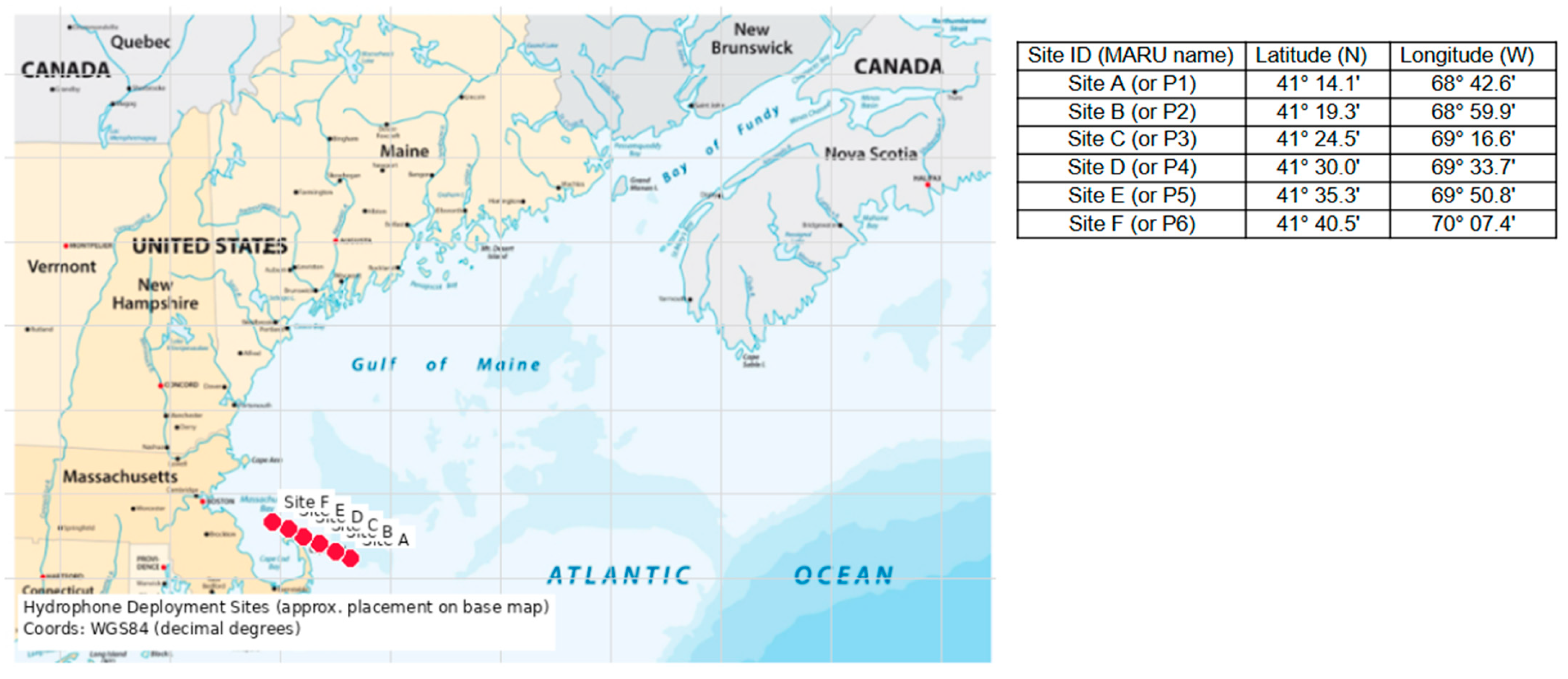
In this study, North Atlantic Right Whale (NARW) vocalization measurements were obtained from the Detection, Classification, Localization, and Density Estimation (DCLDE) 2013 workshop repository (data summary presented in Table 2) [33,34]. The audio recordings—each 15 min in duration and sampled at 2 kHz—were collected using Cornell Marine Autonomous Recording Units (MARUs) [33], with 6 to 10 hydrophones deployed in the Gulf of Maine off the coast of Massachusetts (Figure 2) and spanning the interval from 2000 to 2009. A 2 kHz sampling rate was selected because NARW upcalls occur primarily between 80 and 400 Hz, which is well below the Nyquist frequency of 1 kHz. Furthermore, since this study focuses on investigating NARW upcall detection under low-SNR conditions, prioritizing low-frequency components was appropriate, as these calls dominate the low-frequency band and are most relevant to the research objectives. This choice also reduces memory and computation overhead for long-term monitoring. All recordings (672 audio recordings) were organized into folders by date, and each recording’s filename included its start time. From this repository, 9063 NARW upcall vocalizations of approximately 3 s long were extracted from the audio recordings (and later processed) as per the accompanying annotated files. Additionally, background noise samples—15 min long—used in this study were also sourced from the DCLDE 2013 repository [33].
Given this data source overview, the pre-processing steps are discussed next.

3.2. Data Pre-Processing

The main objective of pre-processing the isolated NARW upcalls (based on known start and end times in the recording—signal and noise) is to improve their suitability for analysis and facilitate their conversion into feature vectors. Pre-processing begins with data partitioning and labeling. To simulate realistic low-SNR conditions, upcalls with specific SNR values are created by first estimating the inherent noise level of each vocalization using its preamble and postamble—segments of the recording that contain only background noise. Additional noise, sampled from ambient measurements at the same upcall location, is then added onto the upcall to achieve a specific SNR level. Following this, the Ideal Binary Mask (IBM) algorithm is applied to determine the SNR threshold at which the upcall can be reliably recovered. The performance of the IBM method is quantitatively evaluated to assess its effectiveness in separating upcalls from noise under varying acoustic conditions. Feature engineering is then performed to extract relevant acoustic characteristics across multiple domains (e.g., time, frequency, and cepstral). Finally, the extracted features are transformed into standardized representations suitable for analysis and model training.

3.2.1. Data Partitioning

Prior to the data pre-processing, the raw dataset (9063 samples) was divided into three distinct subsets—training, validation, and test—using a 70:15:15 ratio, as supported by empirical studies [35,36]. This widely adopted approach in machine learning ensures efficient model development and reliable performance evaluation. Allocating 70% of the data to the training set is important due to the size of the dataset and to ensure sufficient data for model training. The 15% portion allocated to the validation set provided sufficient data for hyperparameter tuning and performance evaluation during training. The last 15% of the data was assigned to the test set, and was used to assess the model’s generalization performance on unseen data.

3.2.2. Data Labeling

Data labeling is a crucial step in data preparation to build the proposed model. To label the SNR-varied data, each null or noise n r ( t ) and vocalization x r ( t ) were tagged as 0 s and 1 s, respectively. These labels enabled the proposed model to make accurate classifications by learning from the labeled SNR-varied data. Following this, the labeled SNR-varied data were created by merging the two with the Python 3.11.9 Pandas dataframe [37].

3.2.3. Upcall SNR Design via Noise Variation

To study the performance of the proposed method across challenging acoustic conditions, a diverse dataset was curated from the 9063 extracted NARW upcalls. This dataset simulates the underwater environment under desired SNR noise ( S N R d ) levels, as expressed in Equation (1):
S N R d [ 10 ,   8 ,   6 ,   3 ,   0 ,   + 3 ,   + 6 ,   + 8 ,   + 10 ]   dB
The generation of the low SNR dataset involves three critical steps: numerical SNR verification, noise generation, and signal superposition.
  • Numerical SNR verification: The SNR is mathematically defined by the ratio of signal power and noise power, which is equivalent to the ratio of their respective root mean square (RMS) amplitudes, as in Equation (2):
R M S n o i s e = R M S s i g n a l 10 S N R d / 20
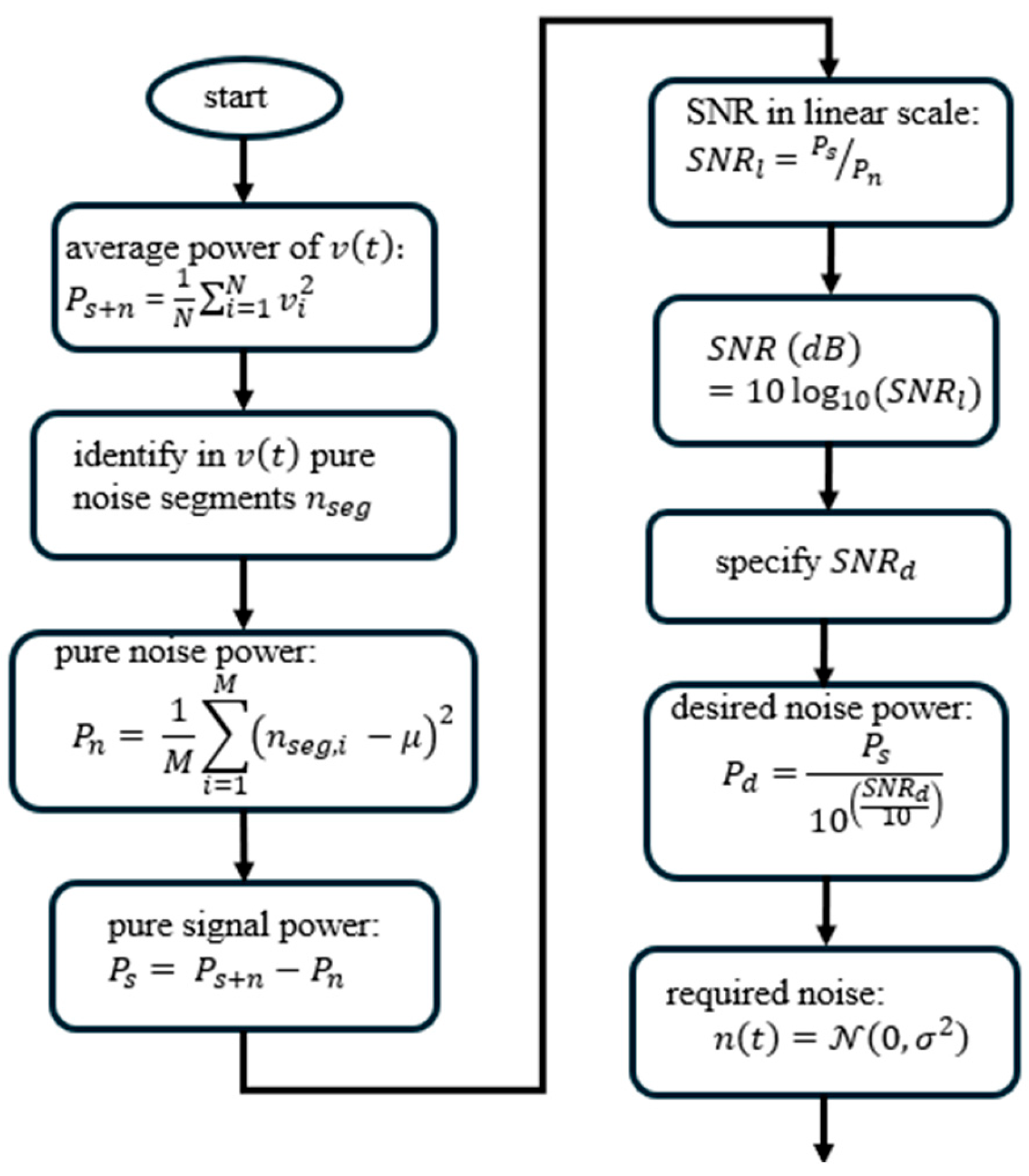
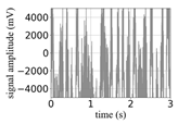
Based on the measured RMS amplitude of the 3 s upcalls R M S s i g n a l , which averaged 0.028011, the background noise component R M S n o i s e was scaled using Equation (2) to achieve the S N R d levels. Using the −10 dB dataset as an example, this calculation mandated that the R M S n o i s e be scaled to an average amplitude of 0.088574 to accurately place the signal 10 dB below the noise floor.
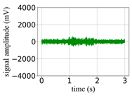
  • Noise generation: The overall process of generating noise is detailed in Figure 3.
  • Signal superposition: The mixed signal x ( t ) is created by superposing the upcall signal ( v t ) and the scaled background noise component ( n ( t ) ), as in Equation (3):
x ( t ) = v ( t ) + n ( t )
By introducing nine varied SNR levels to the NARW audio data, a diverse dataset of 81,567 superposed signals was created ( 9063 × 9   S N R   l e v e l s ). Furthermore, with the IBM method, the 81,567 superposed signals were separated into vocalizations and noise. This implies that 81,567 vocalizations and 81,567 noise were recovered resulting in a total dataset of 163,134 audio files.

3.2.4. Separate Low-SNR NARW Upcalls from Noise: Apply Ideal Binary Mask (IBM)

The IBM method was used to separate the superposed signals (Equation (2)) into their constituent vocalization and noise components [38]. The objective of this process is to evaluate the maximum possible recovery as a function of the controlled SNR. IBM offers a critical advantage over traditional filtering methods, such as Wiener filtering or spectral subtraction, by acting as a perfect time–frequency switch. Unlike those techniques, which apply attenuation factors (partial weights) to noisy frequency bins and often introduce residual noise artifacts, the IBM method is an ideal method for acoustic source separation. It assigns a weight of 1 to bins dominated by the desired signal and 0 to all others. This provides an upper bound on signal separation quality, representing the theoretical limit of source recovery. It applies weights to the frequency bins of the time–frequency representation of the mixed signal. The separation process begins by applying the STFT [39] to the signal Equation (3) to obtain Equation (4):
X t , f = V t , f + N ( t , f )
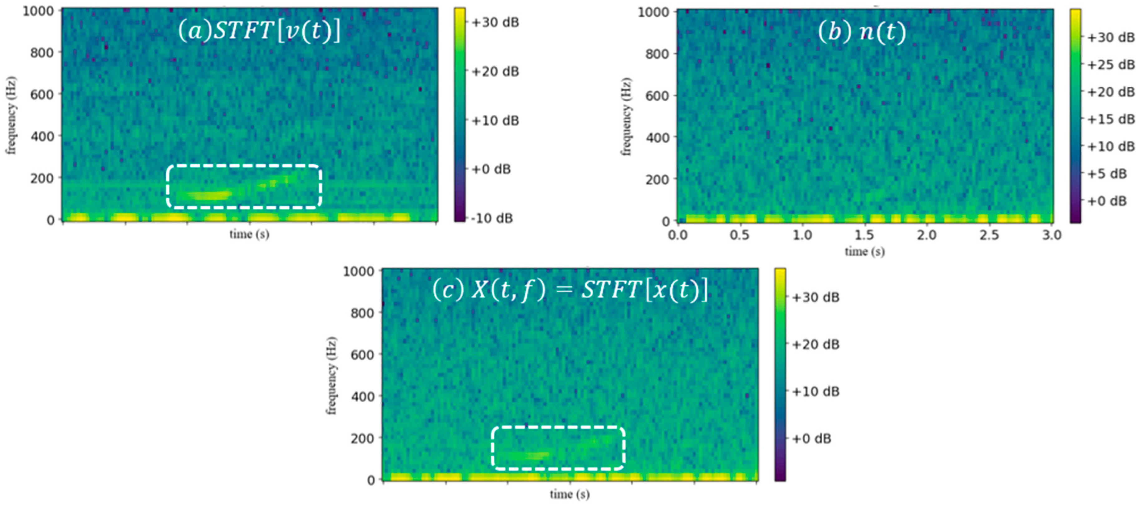
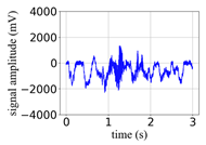
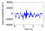
where X t , f ,   V ( t , f ) , and N ( t , f ) are the spectra of x t ,   v ( t ) , and n t , respectively, as shown in Figure 4. The IBM was applied on a per-call basis, it was applied individually to each superposed signal, (a mixture of 3 s upcall and 3 s noise) rather than to continuous audio segments. This approach ensures precise time–frequency alignment and minimizes boundary artifacts. The goal is to assign a weight, w t , f , of 0 to bins containing non-signal frequencies or noise, while assigning a weight of 1 to bins containing vocalizations with energy exceeding the specified threshold as expressed [39] in Equation (5). This matrix is the binary mask.
w t , f =       1                                                                   S N R > t h       0                                                                 o t h e r w i s e .
The binary mask was applied to isolate the desired vocalization signal ( V ^ t , f ) from the superposed signal ( X ( t , f ) ), as shown in Equation (6). The binary mask is a matrix of the same size as the STFT. The STFT of the superposed signals was multiplied element-wise (Hadamard product ( )) with the binary mask that identifies the frequency bins containing the pure signal and those containing pure noise. The binary mask weights (Equation (5)) are applied to X f , t from Equation (4), as expressed in Equation (6):
V ^ t , f = w t , f     X ( t , f )
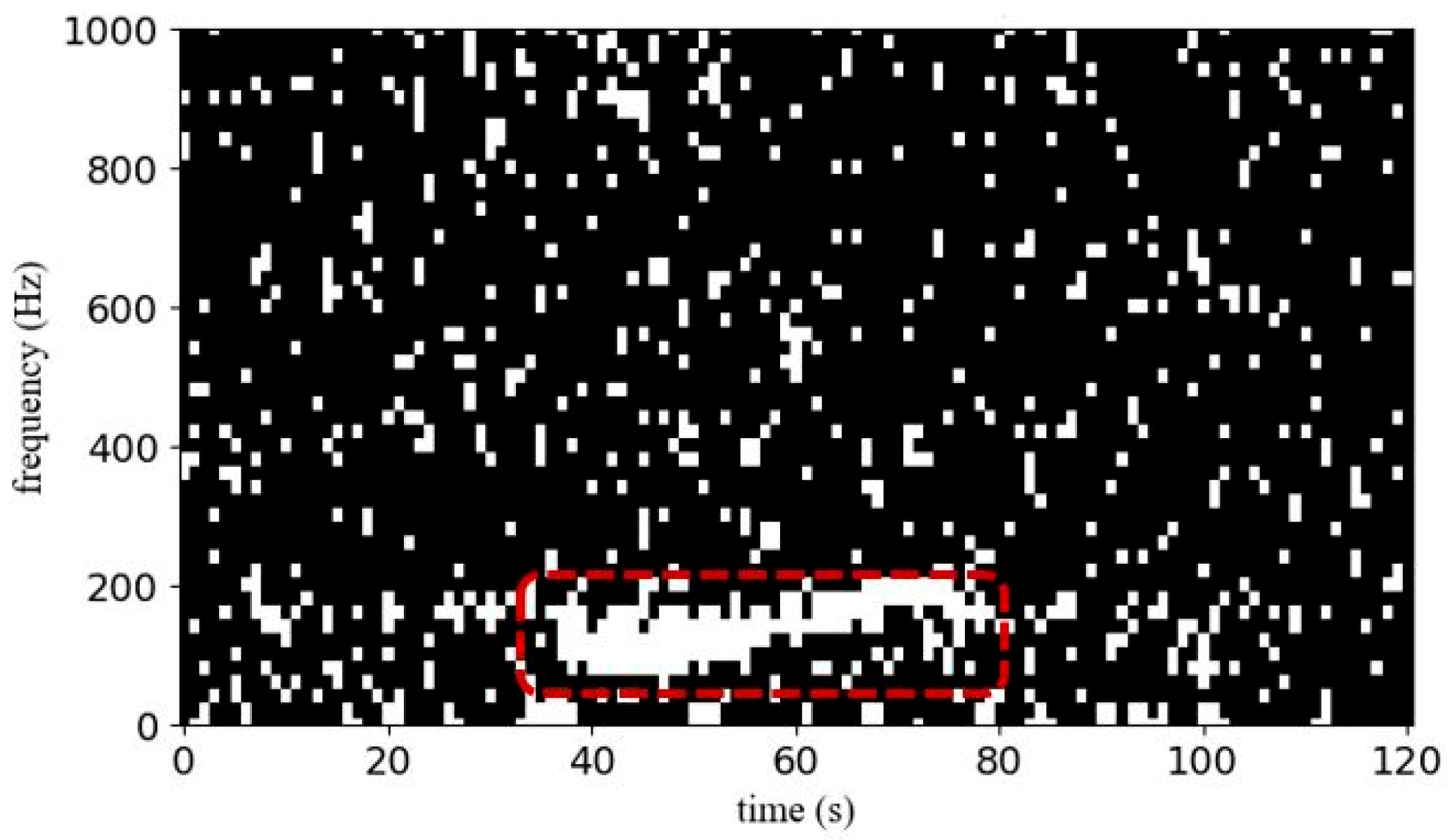
Following this, the vocalization V ^ t , f , as shown in Figure 5, was isilated from noise [40,41]. Afterwards, an inverse STFT (iSTFT) was applied to the resulting product. This process converts the signals ( v r t and n r ( t ) ) back to the time domain using the phase of the superposed signal. Table 3 presents the IBM algorithm.

3.2.5. Evaluating IBM Detection Performance

To measure the computation efficiency and detection quality of the IBM method, two performance metrics were considered: computational time and similarity coefficient ( σ ).
  • Computation Time (CT)
Computation time is a measure of the IBM method’ computationl effort to extract the NARW vocalization signal from noise. This was achieved with the time library in Python. The library uses the time before 1 January 1970 and was called before and after the execution of the IBM. Thereafter, the difference between the end time and the start time was computed using Equation (7):
C T =   t e n d   t s t a r t
where t e n d is the time at which the processing is completed and t s t a r t is the start time. The computation time of the IBM method is compared with the manual method, and the results of this experiment are presented in Table 4.
ii.
Similarity Coefficient ( σ )
Another metric used to evaluate the IBM performance is the similarity coefficient. It measures the degree of similarity between the original and recovered (from the IBM method) upcalls to assess how closely the recovered upcalls match the original ones (Table 5). It is a measure of effectiveness for the IBM recovery process. A high similarity coefficient indicates a well recovered signal. The similarity coefficient is calculated [42] in Equation (8):
σ ( v i ,     V j ) =   | t = 1 n v i ( t )   v r j ( t ) | t = 1 n ( v i ( t ) ) 2     t = 1 n ( v r i ( t ) ) 2  
where σ ( i ,   j )   =   1 indicates high correlation, i.e., i t h   ( V ( t ) ) is the same as the j t h   v ( t ) , and σ ( i ,   j )   =   0 indicates no correlation. The results of this analysis are presented in Table 5.
Table 4 highlights the stark contrast in efficiency between the manual and IBM methods. While the manual approach requires minutes to process even a small number of recordings, the IBM method completes the same task in fractions of a second. Moreover, the manual method does not scale linearly, as human performance declines over extended periods. This substantial reduction in computation time underscores the IBM method’s superior scalability and practical potential for vocalization signal detection.
To ensure the integrity of the results, a check for data leakage was subsequently performed.
iii.
Check for Data Leakage
To prevent data leakage, the raw dataset (9063 samples) was initially partitioned into three distinct subsets (as discussed in Section 3.2.1): training, validation, and test. Data pre-processing was performed independently on each subset to ensure no information from the test or validation sets influenced the training process.
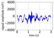
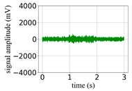
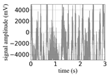
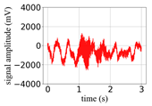
To check for leakage, the recovered upcalls v r t were visualized across SNRs in Table 5. The analysis revealed the patterns of the recovered upcalls varied across different SNRs (column (b)), especially below the noise floor. These variations were attributed to the addition of noise at 9 SNR levels to the original extracted upcalls (9063 audio recordings), resulting in 81,567 superposed signals. Additionally, the correlation between the v t and x t was calculated (column (c)). The low correlation observed between the original and superposed signals, both below and above the noise floor, indicates the absence of data leakage. The recovered upcalls and noise components were subsequently used to train a classifier, so it was essential to confirm that no leakage occurred between the original and processed signals.

3.2.6. Feature Engineering and Analysis of the NARW Upcalls

With data integrity ensured through leakage prevention, the next phase of the analysis focused on feature engineering and statistical evaluation of the SNR-varied acoustic dataset. This phase includes the extraction of relevant features, analysis of skewness, identification of outliers, and investigation of inter-feature correlations.
  • Feature Extraction
To characterize NARW upcalls, 20 acoustic features spanning time, frequency, and cepstral domains were extracted to capture critical vocalization characteristics under low-SNR conditions. A 50 ms frame size with 50% overlap and Hanning windowing was used to balance time resolution and quasi-stationarity assumptions. These features were selected for their relevance to NARW detection and classification. Detailed definitions of the extracted features are provided in Appendix A.
To develop a classification model for low-SNR NARW upcalls, these feature types’ distributions, across all curated upcalls (81,567), were analyzed. To start, these distributions were assessed for skew, to prevent bias. If present, skew must be corrected.
  • Skew Identification
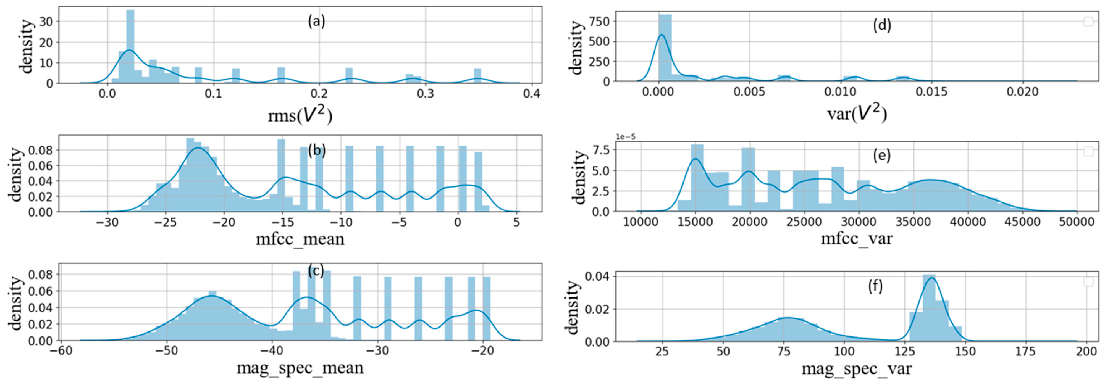
The feature distributions’ means (Figure 6a–c) and variances (Figure 6d–f) across all curated upcalls for the six illustrative features is shown in Figure 6. This analysis identifies patterns in the data to determine a suitable transformation method to rescale the data and reduce its skewness. The robust scaler normalization method will be used.
Additionally, outliers in the features also create bias and their impact must be evaluated.
ii.
Identifying Outliers
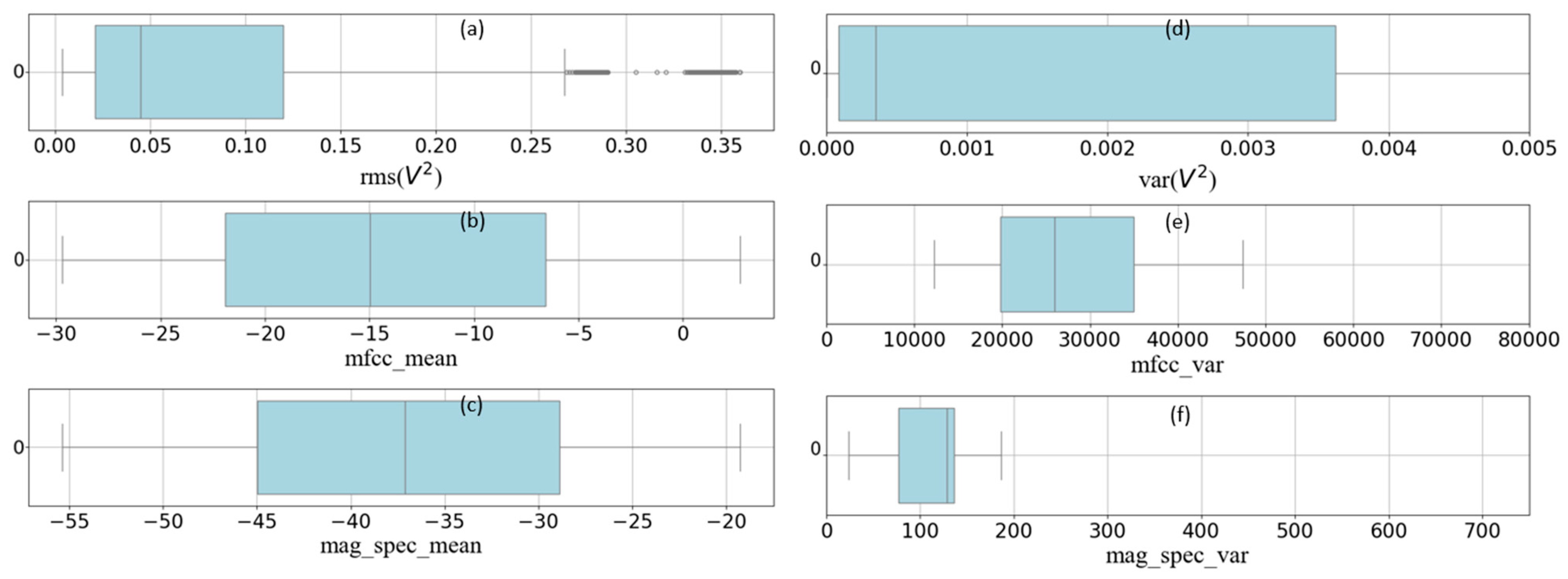
Normally, the presence of data outliers adversely impacts the training of the deep learning models. Typically, outliers are data points that significantly deviate from the features’ distribution. They can distort model performance by skewing the training and lead to inaccurate classification. Therefore, the dataset was examined for outliers. To identify outliers in the SNR-varied acoustic dataset, box plots visualized the features’ distributions, as shown in Figure 7. However, outliers within the feature were retained in this study because the vocalizations have rich spectra that span a wide range and are not considered as outliers.
Consequently, outlier removal is not performed. The Pearson correlation calculated towards this is described next.
2.
Feature Type Correlation Analysis
The inter-feature type correlations were computed using standard Pearson correlation, as shown in Equation (9), to provide insight into the relationships between the independent feature types of the SNR-varied acoustic dataset [43,44]. This analysis also provides a deeper understanding of the dataset, revealing underlying patterns and relationships that might not be obvious.
r   x , y = x i   x ¯ y i y ¯ x i x ¯ 2 y i y ¯ 2
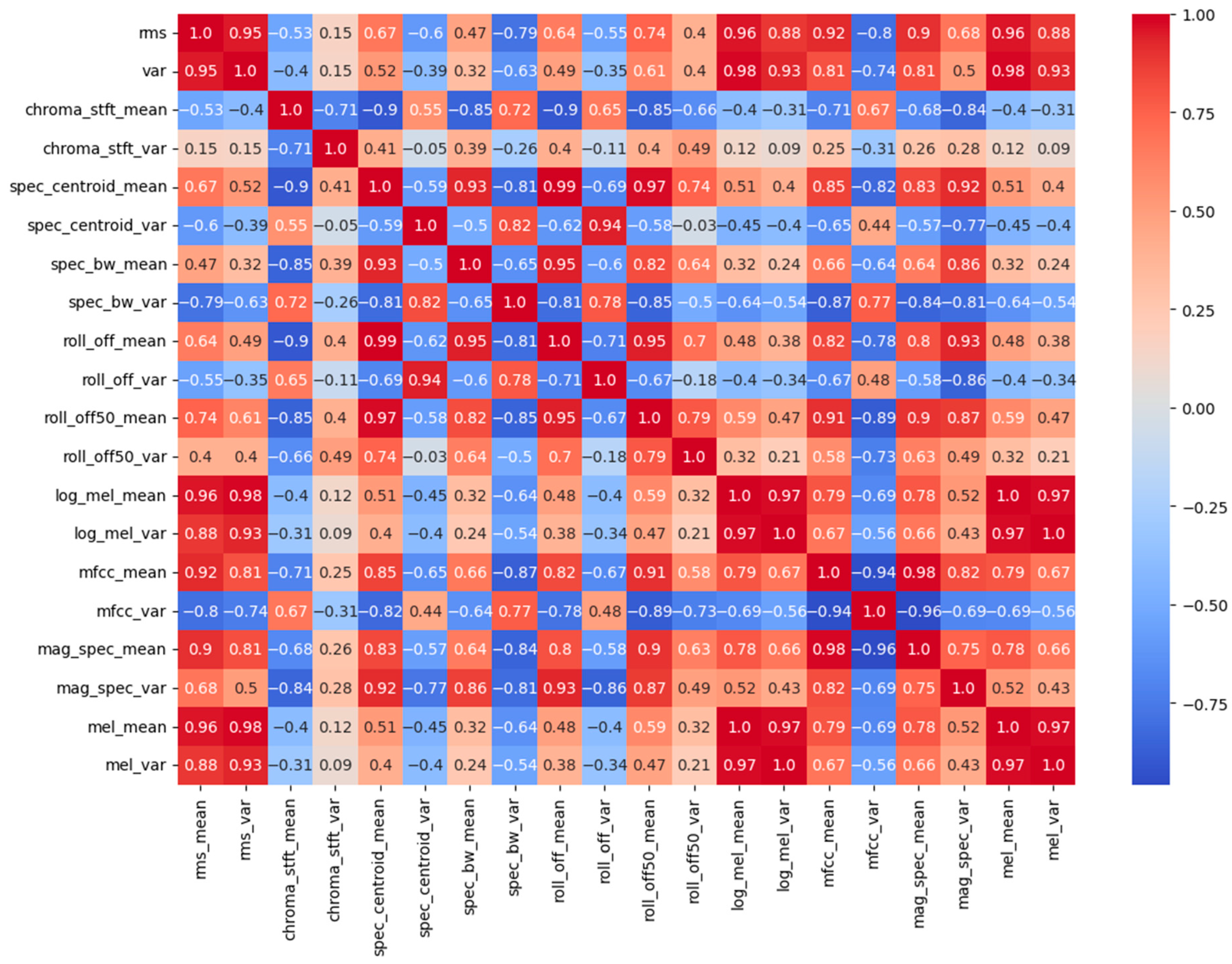
In Equation (9), r ( x , y ) is normalized so it ranges from −1 to 1. A value of 0 indicates no correlation, while −1 represents a negative correlation, and 1 signifies a positive correlation. A heatmap is used to visualize the correlation matrix of the SNR-varied acoustic features in Figure 8.
The correlation across feature types (Table A2) reveals the relationship between the features. While strong correlations can indicate redundancy, these features were preserved because they capture complementary aspects of the signal and may jointly contribute to classification performance under low-SNR conditions. Removing them could risk the loss of subtle but important acoustic cues relevant to NARW upcalls. The analysis of feature correlation (Table A2) primarily provided insights into the upcall features’ physics rather than for feature reduction.
Based on the insights gained from feature engineering and statistical analyses, the next section describes the transformation strategies applied to the SNR-varied dataset to enhance signal quality and analytical robustness.

3.2.7. SNR-Varied Data Transformation

Data skewness and outliers can bias the learning process, especially when feature distributions vary across SNR conditions. To address this, a robust scaler (Equation (10)), which is less sensitive to outliers compared to min-max or standard scaling methods, was used [45,46].
Each 3 s upcall clip is represented by a feature matrix of size (599 frames × 20 features). This dimension is derived from the 50 hop size, resulting in 599 sequential frames across the 3 s duration. The robust scaler normalizes each feature by subtracting its median and dividing by the interquartile range (IQR), computed as Q 3     Q 1 , where Q 1 , Q 2 , and Q 3 are the 25 th , 50 th , and 75 th percentiles, respectively [47,48]. This approach reduces outliers and ensures that features are scaled consistently across clips without enforcing a fixed range, improving robustness under low-SNR conditions [49].
R s   =       x f e a t u r e m e d i a n Q 3 Q 1  
where R s is the normalized correlation value and x is the original value of each feature.
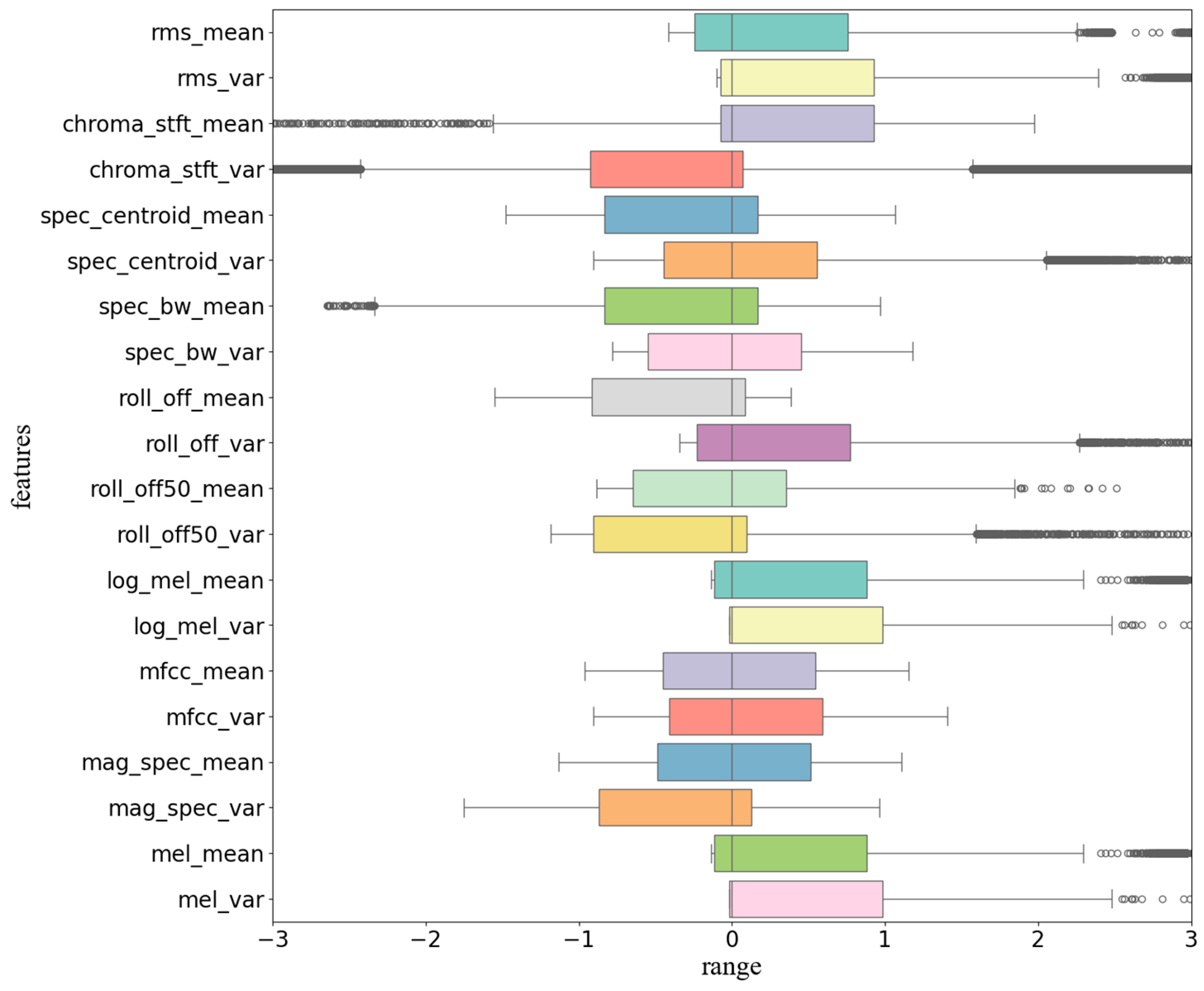
The distribution of the SNR-varied features after normalization is shown in Figure 9. The data transformation process helped to normalize the feature range and reduced their outliers.
This subsection concludes the data pre-processing procedure, such that the data is now able to be classified.

3.3. NARW Upcall Classification Task

The entire set of upcalls (total Q = 9063 ) is denoted Q = { q 1 ,   q 2 , q 3 , …, q Q } such that q i , for i 1 , ,   Q , enumerates the samples. In turn, each q i maps to a feature vector χ i = { x 1 , x 2 , x 3 , …, x M } such that, x m , for m 1 , , M , enumerates the feature types where M is the total number of feature types (20). The mean and variance of each of the following feature types is calculated.
  • root mean square energy (rms);
  • chroma short-time Fourier transform (chroma_stft);
  • spectral centroid (spec_centroid);
  • spectral bandwidth (spec_bw);
  • roll-off (roll_off);
  • 50% roll-off (roll_off50);
  • log mel-spectrogram (log_mel);
  • mel-frequency cepstral coefficients (MFCCs);
  • magnitude spectrogram (mag_spec); and
  • mel-frequency (mel).
The associated class label for each sample is denoted by y m , where y m ∈ {0, 1}. y = 1 denotes class 1 (upcalls); otherwise, it denotes class 0 (noise). The objective is to create a binary classification model using deep learning. This model yields probabilities to classify NARW upcalls, specifically distinguishing between vocalization and noise based on the training data and class labels provided.

3.4. Modeling

This section details the modeling process, including the baseline methods selected to be compared against the proposed IBM-BHN model. It also includes a comprehensive discussion of the proposed method.

3.4.1. Baseline Method

This section presents five state-of-the-art machine learning and deep learning models reported in the literature, which are used as baselines in this work. These methods serve as benchmarks to be compared against the performance of the proposed IBM-BHN approach. This is detailed in the following subsections.
  • Support Vector Machine (SVM)
The SVM finds an optimal hyperplane which separates data points (support vectors) into different classes. It maximizes the margin between support vectors by transforming data from a lower- to a higher-dimensional space. The SVM finds an optimal hyperplane that separates data points (support vectors) into different classes. The architecture of the SVM-based NARW vocalization classification model proposed by Ibrahim et al. [19] was modified in this study. This architecture was chosen based on its superior performance in NARW vocalization classification, which can be attributed to its effective use of MFCC and DWT feature representations. These features enhance the model’s ability to capture the complex patterns in marine mammal vocalizations, leading to improved classification accuracy.
2.
Artificial Neural Networks (ANNs)
The ANN consists of interconnected layers that enable unidirectional information flow from the input to the output layer. The densely connected layers process data through hidden units, allowing the model to comprehend the patterns in the input SNR-varied data. The study reported on here modified and used the ANN architecture proposed by Pourhomayoun et al. [20] due to its proven performance, which could be attributed to their effective use of the time and frequency domain feature extraction methods (such as duration, number of pulses, average bandwidth, and center frequency). The model’s ability to process complex patterns through densely connected layers makes it particularly suitable for classifying marine mammal vocalizations. Comparative studies in [20] revealed that the ANN model proposed by Pourhomayoun et al. performs better than other models in similar contexts (other studies that considered marine mammal vocalization detection and classification), making it a good reference in terms of performance for this study.
3.
Convolutional Neural Network (CNN)
CNNs are neural networks composed of multiple layers, including the input layer, convolutional layers, pooling layers, and fully connected layers. The input layer accepts the vector representation of the data; convolutional layers apply filters to classify local patterns; pooling layers down-sample feature maps; and fully connected layers perform classification based on the learned features. The proposed CNN architecture by Wang et al. [23] was selected and modified in this study because of its proven effectiveness in previous research. The model’s ability to classify local patterns through convolutional layers and reduce dimensionality through pooling layers makes it suitable for classifying marine mammal vocalizations. Additionally, the use of multi-scale waveforms and log-mel spectrograms with delta features (such as MFCC) enhances the model’s capability to capture the rich spectral and temporal patterns in whale calls. Comparative studies [23] demonstrated that the CNN model outperformed other models in similar applications, establishing it as a good reference for evaluating performance in this study.
4.
Long Short-Term Memory (LSTM)
The LSTM architecture includes an input layer that accepts vector representations of the data; an LSTM layer that processes data in one direction; a flatten layer that converts the LSTM output into a 1D vector; a dense layer that learns complex patterns; a dropout layer to prevent overfitting; and an output layer that generates the model’s classification probability. The LSTM architecture proposed by Duan [27] was selected and modified in this study because it allows adaptability, which is crucial for addressing the specific needs of this study. Duan’s method involves filtering the vocalizations to remove noise and enhance line-shaped clicks, followed by the use of line classification to extract their features. This method also involves the generation of spectrograms. This approach improves the performance of the model by ensuring that the features are clean and focused on the relevant signal characteristics, thereby enhancing the model’s ability to accurately classify vocalizations. Comparative studies [27] revealed that Duan’s LSTM model outperformed traditional marine mammal classification models, making it a good benchmark against performance for this study.
5.
Residual Neural Networks (ResNets)
ResNets are deep neural networks that address the vanishing gradient problem during training. They introduce skip connections (also known as identity mappings) that allow information to flow directly from one layer to another without being transformed. This helps prevent degradation of performance as the network deepens. The ResNets architecture is composed of an input layer, an initial layer, eight residual blocks, a global average pooling layer, and a fully connected layer. The ResNet architecture proposed by Kirsebom et al. [25] was modified and used in this study. This architecture was selected due to its flexibility and ability to be tailored towards the classification of marine mammal vocalizations. In addition, the model’s ability to maintain performance as the network deepens through skip connections makes it particularly suitable for classifying marine mammal vocalizations. Kirsebom et al.’s method involves training the ResNet on time–frequency representations of the NARW upcalls, specifically using spectrograms. This approach enhances the model’s ability to capture complex patterns in the vocalizations, leading to improved classification accuracy. Comparative studies [25] revealed that the ResNet model outperformed traditional classification methods, making it a good reference for evaluating the performance for this work.

3.4.2. Proposed IBM with the BiLSTM–Highway Network (IBM-BHN) Method

The IBM-BHN method is a novel NARW vocalization classifier that aims to address the limitations of existing models; it was specifically developed to classify NARW vocalizations in low-SNR scenarios. It combines the strengths of the BiLSTM and highway networks to better classify NARW vocalizations from noise, improve the accuracy performance over existing models, and optimize the flow of information in the network to achieve near real-time classification. The complete data flow for the IBM-BHN model, from the SNR-varied data to the final classifier, is summarized in Figure 10.
The architecture of the proposed IBM-BHN (the classification component is shown in the final stage of Figure 11) consists of the input layer, a BiLSTM layer, a highway layer, a flatten layer, a dense layer, a dropout layer, and the classification layer, as discussed in subsequent subsections.
1.
Input Layer
The input layer of the proposed IBM-BHN method takes the pre-processed SNR-varied acoustic data sequence as the input. The output of this layer was fed into the next layer.
2.
BiLSTM Layer
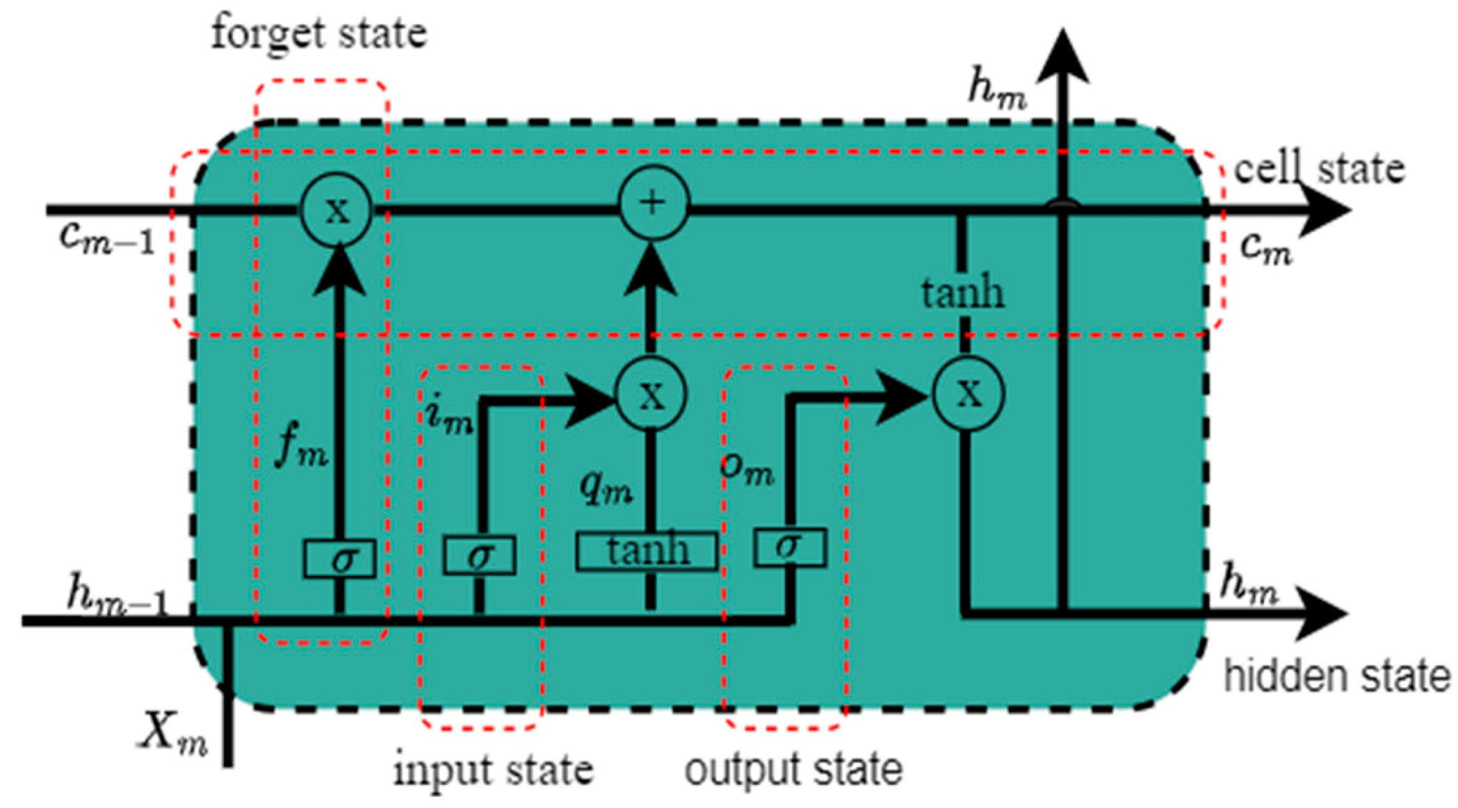
BiLSTM is a powerful variant of RNNs. It excels at capturing long-term dependencies between time steps in sequences especially time-series data [50]. It processes input sequences bidirectionally, capturing complex details and relationships from both past and future time steps [51]. This capability allows it to model complex, nonlinear patterns and temporal dependencies [52]. The BiLSTM layer employs two LSTMs: one reads the input sequence forward; the other reads it backward [53]. A standard LSTM cell manages information flow using three primary gates: input gate i (which controls new memory content); forget gate f (which regulates memory retention); and the output gate o (which modulates the information passed to the next layer). Other gates include the cell activation vector c and the hidden gate h , as discussed in [54] and [55]. The cell activation vector includes modulated new memory q , and partially forgotten previous memory ( c m 1 ) , while the hidden gate combines the cell activator vector and the output gate. The internal mechanics of the LSTM cell are conceptually shown in Figure 12.
Based on the standard LSTM equation in [56], the BiLSTM equation can be expressed by Equations (11)–(13) as follows:
h m   =   L S T M   ( h m 1 ,     X M ) ,                   m     [ 1 ,   , M ]    
h m = L S T M   ( h m 1 ,     X M ) ,                   m     [ 1 ,   , M ]    
g m = h m h m  
where h m 1 and h m 1 are the hidden layer state of the forward and backward LSTM for the time step m − 1.   X m is the input to the LSTM cell at time step m while g m is the contextual representation of the SNR-varied data   X m at time step m. The BiLSTM concatenates the outputs of the forward and backward LSTMs to form a comprehensive contextual representation of the SNR-varied data, which is then fed into the highway layer.
3.
Highway Network Layer
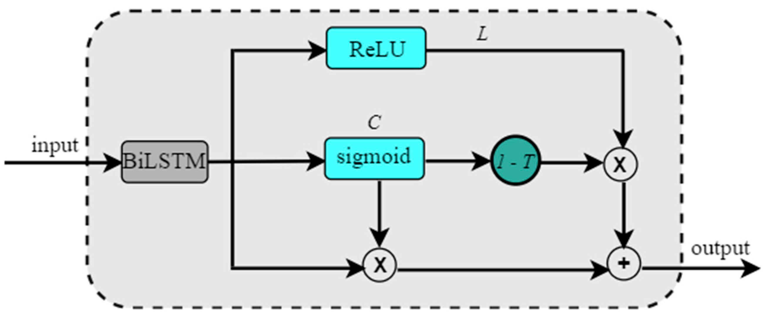
The highway layer optimizes information flow by refining features from the BiLSTM layer using two gates: the transformation gate ( T ) , which applies an ReLU function to the BiLSTM output to manage information transformation, and the carry gate ( C ) , which uses a sigmoid function to determine information retention. The outputs of these gates (denoted as L and 1 − T, respectively) are multiplied element-wise and summed with the BiLSTM output to produce the highway layer output as shown in Figure 13. This process enhances feature refinement and optimizes information flow [57]. Additionally, relevant input information is learned, and irrelevant details are suppressed. The resulting output is expressed in Equations (14) and (15) as follows:
T =   σ W T g   +   b T
U = T f W g g + b g + ( 1 T ) g
where W T , W g , b T ,   b g , and U represent the weight matrix, bias vectors, and the output of the highway network, respectively. This output is then passed to the flatten layer.
4.
Flatten Layer
The flatten layer transforms the three-dimensional (3D) tensor from the highway layer into a one-dimensional (1D) vector. This transformation prepares the data for processing by densely connected neurons. The resulting 1D vector is then passed to the subsequent dense layer.
5.
Dense Layer
The flatten layer output was input into the dense layer. The dense layer extracts more informative representations by introducing nonlinearity. Each cell in the dense layer computes a weighted sum of the input features using the hyperbolic tangent (tanh) activation function, mapping input values to a range between −1 and 1. This nonlinearity enhances the model’s ability to learn complex patterns, improving its performance in classifying NARW vocalizations. To control model complexity and reduce overfitting, an L2 regularization strategy was applied. This strategy adds a penalty term to the cost function proportional to the squared magnitude of the model’s weights, encouraging smaller weight values. The cost function measures how well the model’s classifications match the actual labels during training, with the goal of minimizing this function to improve model performance. The cost function with L2 regularization is expressed in Equation (16):
c o s t   f u n c t i o n   =   l o s s + λ 2 χ i   | | w | | 2
In Equation (16), the loss refers to the original loss function without regularization. The parameter λ determines the regularization strength, while χ i is the number of features or coefficients. The variable w denotes the weight of each feature, and | | w | | 2 signifies the sum of the squares of all feature weights (model weights) [58]. The output from this layer is subsequently passed to the dropout layer.
6.
Dropout Layer
To prevent overfitting and improve generalization on unseen data, the IBM-BHN method incorporates a dropout layer [58]. During training, the activations (features) of the selected BiLSTM cells are set to zero, and the remaining cells adapt to compensate for the missing ones, resulting in a more robust model. This randomness prevents the network from over-relying on specific connections and reduces overfitting [59]. The output of this layer is then fed into the classification layer.
7.
Classification Layer
The classification layer in the proposed method is a fully connected layer employing a sigmoid activation function to generate the final model output for SNR-varied acoustic data. Each neuron is activated using the tanh function. This layer’s output is the probability of classifying NARW vocalizations from noise. The pseudo-code for the IBM-BHN NARW algorithm for NARW upcall classification is summarized in Table 6.

3.5. Hyperparameter Settings

Hyperparameter tuning was conducted using random search optimization and a three-way holdout procedure. This procedure was also applied to the five baseline models to select the best model for comparison purposes. The tuning was performed on both training and validation datasets. During this process, a combination of hyperparameter settings was used to create a model in each iteration and fit on the training data with labels. The performance of these models was evaluated on the validation set. Then, the hyperparameter settings associated with the best performed model are chosen to train the proposed model, as shown in Table 7.

3.6. Model Training, Validation, and Testing

The best hyperparameter values selected through the hyperparameter tuning procedure were used for model training. The validation dataset helped to assess model performance during training. To evaluate the ability of the model to generalize to unseen data, the trained model was tested on the test dataset. Detailed discussions on training, validation, and testing are provided in the following subsections.

3.6.1. Model Training

The model was compiled with an Adam optimizer, a specified learning rate, binary cross-entropy loss, and an accuracy metric. The Adam optimizer adjusted the model’s parameters, while the learning rate controlled the adjustment speed at which the model’s internal parameters (weights and biases) are adjusted. Binary cross-entropy calculates the error rate between the classified and actual labels, guiding the model toward optimal parameter values. Accuracy evaluates the performance of the model. The model was trained on the training dataset over 50 epochs. Data was processed in batches of 96 until completion.

3.6.2. Model Validation

During training, the validation dataset was used to evaluate the performance of the model. This was achieved by comparing the classified labels with the actual labels and computing the loss rate and accuracy of the model. If the model performs poorly on the validation set, then it may not be able to generalize well to the test set, which could be an indication of overfitting.

3.6.3. Model Testing

To provide an unbiased evaluation of the proposed model, an unseen test dataset was used. This test dataset was not previously used in the training and validation. The model’s performance was examined on this unseen test dataset to evaluate its performance in real-word scenarios [60].

3.7. Model Evaluation

To assess the performance and generalizability of the proposed IBM-BHN model, a comprehensive evaluation was conducted using both standard classification metrics and statistical significance testing. This approach ensures that observed performance gains are not only quantitatively measurable but also statistically meaningful when compared to baseline models.

3.7.1. Metrics

The proposed IBM-BHN and baseline models were evaluated with standard metrics such as accuracy, precision, specificity, sensitivity, F1-score, false positive rate (FPR), and false negative rate (FNR).

3.7.2. Statistical Significance Testing

To evaluate whether the proposed model significantly differs from the baselines, the McNemar’s test was employed. This test is well-suited for comparing multiple classifiers on the same dataset with a single holdout set [61] and it provides insight into the generalizability of the models. McNemar’s test is based on a 2 × 2 contingency table that records the number of samples where the proposed model and the baseline model agreed or disagreed with the ground truth, as described in Table 8.
Under the null hypothesis, the two algorithms should have the same error rate, i.e., n 01 =   n 01 . McNemar’s chi-square statistic with continuity correction is calculated in Equation (17) as follows:
χ 2   =   n 01   n 10   1 2 n 01 +   n 10
where the subtraction of 1 in the numerator accounts for continuity correction, since the test statistic is discrete while the chi-square distribution is continuous. The resulting statistic follows a chi-square distribution with 1 degree of freedom. A p -value less than the significance threshold   = 0.05 indicates that the proposed model performs significantly differently from the baseline. To complement the statistical test, the effect size ψ was reported to quantify the magnitude of differences between the proposed model and the baseline models.

4. Results

This section presents the results from the experiments performed on the classification of NARW upcalls. The results are based on the unseen test dataset containing 12,303 upcalls and 12,303 underwater acoustic ambients (noise) totaling 24,606 audio recordings from the IBM-BHN method. The section is divided into two main parts: an analysis of the extracted feature characteristics, and the subsequent classification performance evaluation across varied SNR conditions.

4.1. Training and Learning Curves

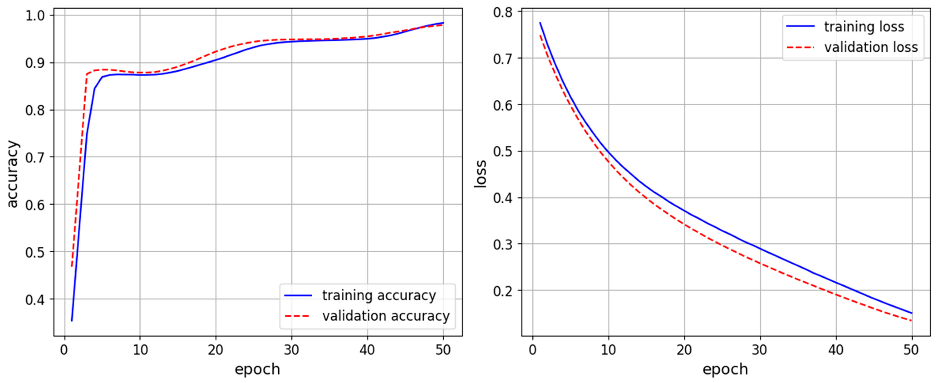
To evaluate the performance and generalization capability of the proposed IBM-BHN model, the training and learning curves across 50 epochs were analyzed. These curves provide insight into the model’s convergence behavior, overfitting control, and overall learning dynamics. As shown in Figure 14, the training curves plot the accuracy of the model on both the training and validation datasets over successive epochs. The training accuracy reflects the model’s ability to learn from labeled data, while the validation accuracy assesses its performance on unseen data. Both curves exhibit consistent improvement with no substantial divergence, indicating stable generalization. Notably, the validation loss remained lower than the training loss throughout, which is consistent with the application of regularization techniques such as dropout (rate = 0.5) and L2 regularization ( λ   = 0.001). This trend demonstrates that the model successfully mitigated overfitting [59] and maintained robust predictive performance on unseen validation data.

4.2. Performance of IBM-BHN for NARW Upcall Classification vs. Five Baseline Models

The IBM-BHN method was evaluated for NARW upcall classification and compared against the following baseline models: SVM, ANN, CNN, ResNet, and LSTM. Key performance metrics such as accuracy, precision, sensitivity, and F1-score are compared to highlight IBM-BHN’s effectiveness in distinguishing upcalls from underwater acoustic ambient noise. IBM-BHN consistently outperformed most of the five baselines, as shown in Table 9. The sensitivity metric of IBM-BHN is marginally lower than those of SVM, ANN, and ResNet, which means there may be misclassifications of upcalls as noise. However, IBM-BHN’s consistently high performance across accuracy, precision, and F1-score parameters underscores its overall efficiency in NARW upcall classification. McNemar’s test revealed statistically significant differences between the proposed IBM-BHN and all baseline models (Table 10). Across comparisons, p-values were consistently below 0.001, and the corresponding effect sizes ψ 0.75 indicated large practical differences in performance, underscoring the robustness of the IBM-BHN model.
The advantage of the proposed method over the baseline models stems from the architectural strengths of IBM-BHN: The BiLSTM component processes acoustic feature sequences bidirectionally, preserving temporal coherence in noisy spectra. This is particularly important for detecting subtle patterns in low-SNR conditions, where conventional models may lose contextual information. Additionally, the highway network layer facilitates deeper learning by allowing critical, less-noisy features to propagate through the network without degradation.

4.3. Receiver Operating Characteristic (ROC) Assessment: Proposed IBM-BHN Model vs. Baseline Models

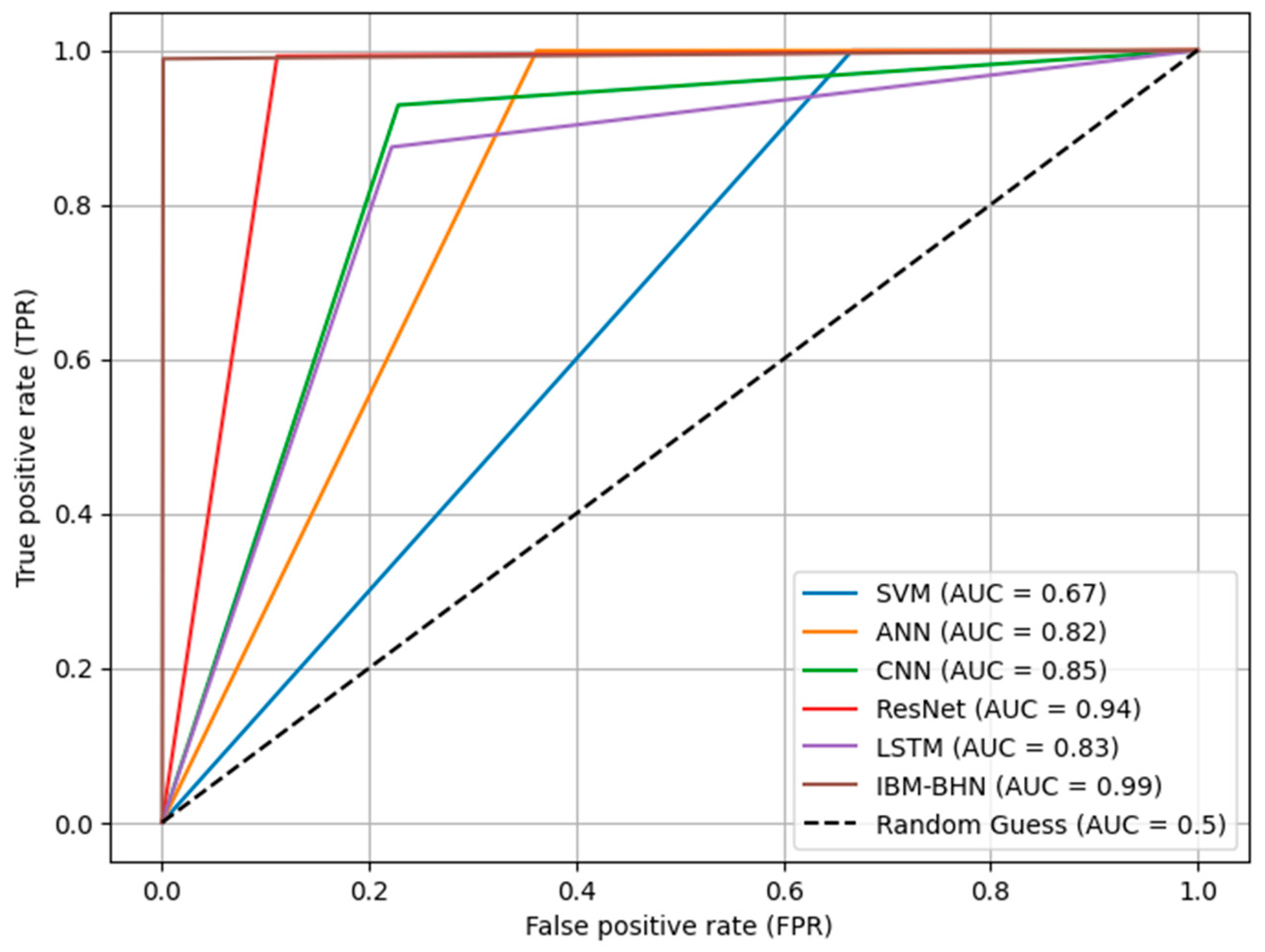
To further evaluate the IBM-BHN method, Figure 15 compares the receiver operating characteristic (ROC, i.e., TPR vs. FPR) curves for IBM-BHN and the baseline models considered (SVM, ANN, CNN, ResNet, and LSTM). Each ROC curve is associated with an area under the curve (AUC), reflecting the model’s ability to distinguish NARW upcalls from noise. The proposed IBM-BHN method (brown) achieved the highest AUC of 0.99 (legend). This means the IBM-BHN distinguishes NARW from underwater acoustic ambient (noise) with the lowest error. This superior performance is attributable to the architectural design of the IBM-BHN model. The BiLSTM layer captures temporal dependencies in both forward and backward directions, enabling the model to retain contextual continuity even when the input signal is degraded by noise. Complementing this, the highway network facilitates seamless transmission of salient features through deeper layers, preventing information bottlenecks and allowing the classifier to fully exploit the representations generated by the preceding IBM pre-processing stage.

4.4. Error Analysis Comparison of IBM-BHN and the Five Baseline Models Considered

Table 11 presents an error analysis comparing IBM-BHN with SVM, ANN, CNN, ResNet, and LSTM with the false positive rate (FPR) and false negative rate (FNR). SVM and ANN exhibit high FPRs (40% and 27%, respectively) but low FNR (0.1%), indicating frequent misclassification of background noise as upcalls, while rarely misclassifying true upcalls. CNN (20% FPR, 8% FNR) and LSTM (20% FPR, 14% FNR) exhibit the same FPR and low FNRs. The high FNRs for both models indicate they misclassify a substantial number of true upcalls. Meanwhile, the ResNet model stood out for its notable performance, achieving a low 10% FPR and a lower 0.1% FNR, indicating the ability to correctly classify true positives. Comparatively, IBM-BHN outperformed all considered baselines in terms of FPR, achieving the lowest rate at 0.09%. Its FNR (1%) was slightly higher than SVM, ANN, and ResNet, but still exhibits a robust classification capability, missing very few actual upcalls.
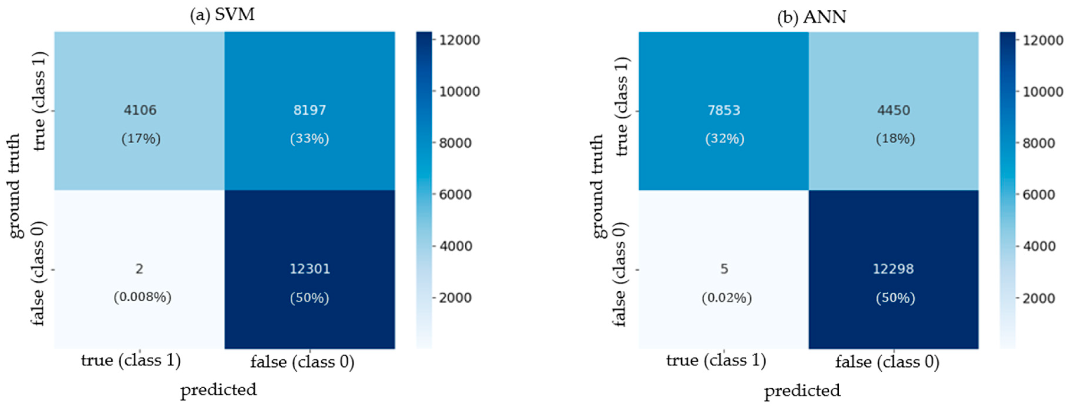
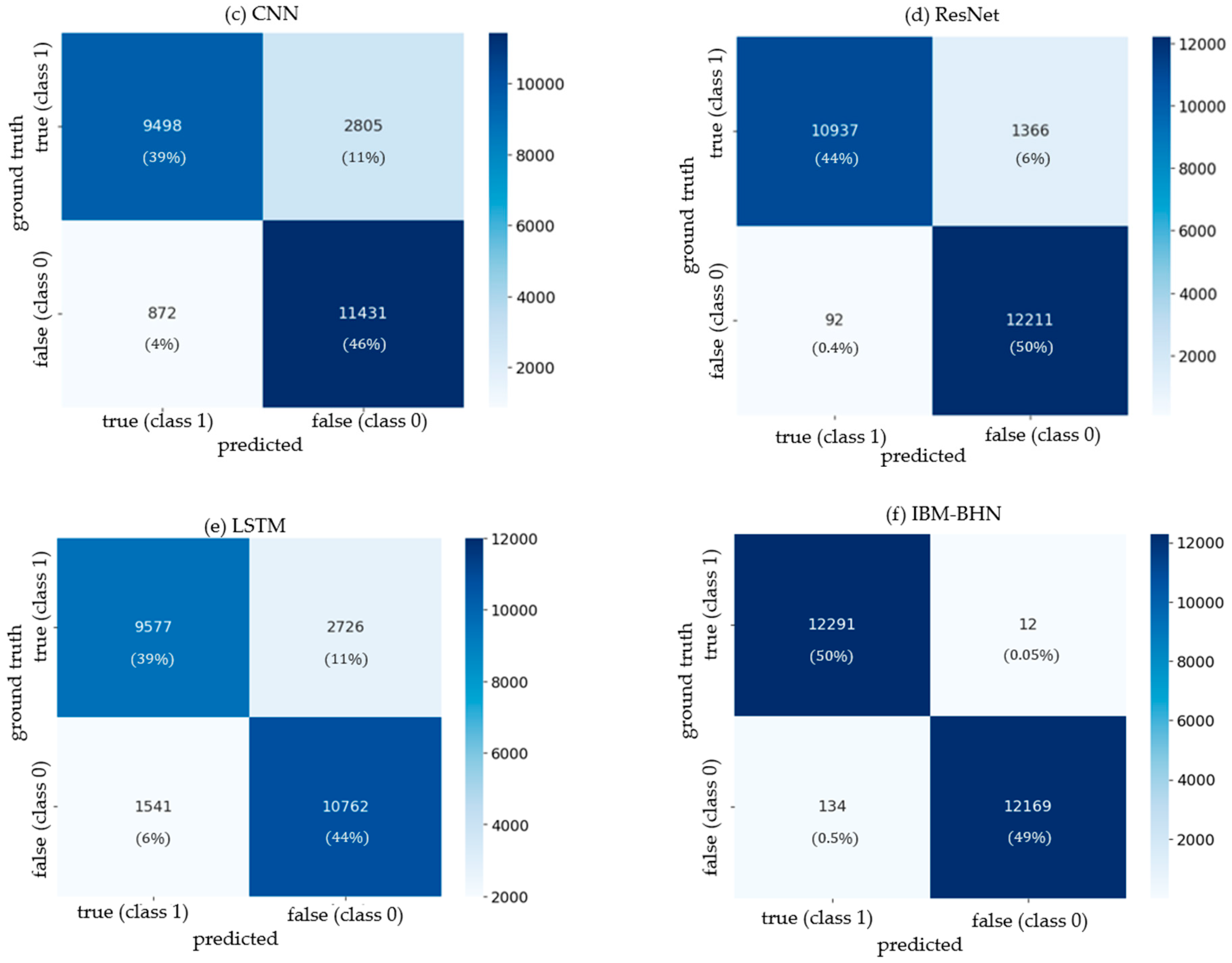
Confusion matrices for SVM, ANN, CNN, ResNet, LSTM, and IBM-BHN are compared in Figure 16. The diagonal elements represent correctly classified NARW upcalls and noise, while off-diagonal elements indicate misclassifications.
To begin, the SVM model shown in Figure 16a correctly classifies 4106 instances as upcalls (true positives (TPs)), with 8197 misclassifications as upcalls (false positives (FPs)). It also correctly classified 12,301 instances as noise (true negatives (TNs)), with only 2 misclassifications of upcalls as noise (false negatives (FNs)). While the ANN model in Figure 16b correctly classified 7853 TP, with 4450 FP, and 12,298 TN, with 5 FN.
The CNN model in Figure 16c achieved 9498 TP and 2805 FP, while correctly classifying 11,431 noise instances (TN) and misclassifying 872 upcalls (FN). In comparison, the ResNet model in Figure 16d reveals 10,937 correctly classified upcalls (TP), 1366 FP, 12,211 TN, and 92 FN.
Furthermore, the LSTM model in Figure 16e revealed 9577 TP and 2726 FP, along with 10,762 TN and 1541 FN. Lastly, the proposed IBM-BHN model in Figure 16f demonstrates a remarkable performance compared to all the considered baselines, correctly classifying 12,291 upcalls (TP) with only 12 FP, and 12,169 TN with 134 FN. The observed performance improvement stems from the model’s hybrid feature representation, which integrates temporal, spectral, and cepstral characteristics to capture complementary acoustic information. Moreover, the combined use of BiLSTM and highway network components strengthens the model’s learning capacity.

4.5. Comparison of Response Time: Proposed IBM-BHN vs. Baseline Models

The proposed IBM-BHN and baseline models were also evaluated for their computation efficiency specifically, response times. As shown in Table 12, IBM-BHN outperforms the baseline models, demonstrating greater efficiency. Notably, the proposed IBM-BHN model demonstrates a good response time in classifying NARW upcalls. This accomplishment is impressive given the computation constraints of BiLSTM algorithms. The IBM-BHN model classified the unseen (independent) test NARW upcalls within 1 s (with the computer described in Section Computation Time (CT)). This improvement in response time is attributed to the additional implementation of the highway network mechanism, which optimizes the information flow in the network.

4.6. Impact of BiLSTM Units on the IBM-BHN Classifier

To further understand the proposed method’s performance, an investigation into the impact of varying the number of BiLSTM units on the classification of NARW upcalls was conducted. The findings are summarized in Table 13. Across these experiments, varying the number of BiLSTM units from 16 to 96 had no substantial impact on the IBM-BHN’s classification capabilities. This stability may be attributed to the architectural robustness of the IBM-BHN model, which effectively leverages its hybrid feature representations and noise-aware pre-processing to maintain reliable performance across a range of BiLSTM units.

4.7. Impact of Imbalanced Evaluation Test Dataset on False Positive and Negative Rates Performance

The test dataset used was class-balanced (equal number of positive and negative samples), as most models will not perform optimally with an imbalanced test dataset. However, performance under an imbalanced dataset is common in real-world applications. Testing against an imbalanced dataset examines the model’s resilience to real-world conditions. Therefore, the models’ performances were evaluated using a skewed test dataset containing 5000 upcalls and 10,000 noise instances. This setup, biased toward noise, allowed analysis of false positive and false negative rates across both the proposed IBM_BHN and baseline models. The results of this analysis are presented in Table 14.
SVM exhibits the highest false positive rate (86%) and a zero false negative rate (0%), indicating frequent misclassification of noise as upcalls while successfully identifying all true upcalls. Similarly, ANN exhibits a high false positive rate (67%) and a zero false negative rate (0%), reflecting a strong tendency to misclassify noise but highly effective at identifying upcalls.
CNN showed a moderate false positive rate (23%) compared to SVM and ANN, but a much higher false negative rate (13%), suggesting fewer noise misclassifications along with a notable number of missed upcalls. ResNet demonstrates a relatively low false positive rate (7%) compared to CNN, and a low false negative rate (6%), offering a more balanced performance than SVM and ANN, though misclassifications remained present in both classes.
LSTM shows a false positive rate of 14% and the highest false negative rate (16%) among all models, indicating reduced reliability in classifying actual upcalls. In contrast, the proposed IBM-BHN model achieved superior performance, with a false positive rate of 6%, lower than all baselines, and a zero false negative rate (0%). These results highlight IBM-BHN’s effectiveness in minimizing false alarms while reliably classifying NARW upcalls under imbalanced conditions. The IBM-BHN is resilient to the considered imbalanced test dataset which is biased to noise—a real-world condition. This improvement can be attributed to the model’s complementary hybrid feature representations, which effectively capture rich temporal, spectral, and cepstral characteristics of the upcalls. Additionally, the BiLSTM architecture’s ability to model bidirectional temporal dependencies enables the network to maintain contextual continuity across time, allowing it to distinguish subtle upcall patterns even under class imbalance conditions.

4.8. IBM-BHN Performance Under Diverse Noise Conditions

To evaluate the resilience of the IBM-BHN model under varying noise conditions, its classification performance was assessed across a range of SNRs, as summarized in Table 15. This analysis quantifies the impact of noise levels on the model’s ability to accurately classify NARW upcall learned patterns.
At SNRs above the noise floor (10 dB, 8 dB, and 6 dB), the model achieves 0% false positive and false negative rates, suggesting a definitive classification when the upcall signal strength is greater than the background noise.
As the SNR decreases to 3 dB and 0 dB, the performance begins to degrade. At 3 dB, the false negative rate rises slightly to 0.1%. At 0 dB, it reached 0.4%, suggesting occasional misclassification of upcalls as noise. Notably, the false positive rate remained at 0% over this range, indicating no misclassification of noise as upcalls.
Below the noise floor (−3 dB to −10 dB), where noise levels exceed the signals, performance declined. At −3 dB, the false negative rate increased to 0.9%, reaching 4.3% at −10 dB. The false positive rate also increased, from 0.1% at −3 dB to 0.5% at −10 dB, indicating a growing tendency to misclassify noise as upcalls under extreme conditions.
Despite this degradation, the IBM-BHN model maintained reasonable sensitivity in high-noise environments. For instance, at −10 dB SNR, where the signal is ten times weaker than the noise, the model still achieved low false positive rates of 0.5% and false negative rates of 4.3%. These results demonstrate the model’s robustness and its ability to maintain reliable classification performance under adverse acoustic conditions. This resilience stems from its integrated use of temporal, spectral, and cepstral feature representations, which collectively capture complementary aspects of the upcall signal. Rather than relying on a single feature domain that may be susceptible to noise corruption, the model synthesizes information across multiple acoustic domains, enabling it to detect upcalls even when individual features are partially degraded.

5. Discussion

This section presents a performance assessment of the classifier developed for NARW upcall classification, including comparisons between the proposed IBM-BHN model and the five baseline methods. The ROC curve analysis and the role of BiLSTM units in capturing temporal dependencies and the contribution of the highway network to information flow and classification accuracy are examined. Classification errors are analyzed to highlight model limitations and strengths. The section concludes with a summary of potential directions for future research.

5.1. Training and Learning Curves

To ensure the robustness and generalizability of the proposed IBM-BHN model, the learning curves (Figure 14) were analyzed to assess overfitting control. These curves illustrate successful control of overfitting: the training and validation loss curves track closely throughout all 50 epochs, exhibiting a stable and narrow train-validation gap. Moreover, the continued decrease in validation loss without divergence confirms the effectiveness of the applied regularization techniques—specifically dropout and L2 regularization—in mitigating overfitting. Together, these trends indicate that the model maintained stable generalization and is well-suited for unseen data.

5.2. Performance of IBM-BHN for NARW Upcall Classification vs. Five Baseline Models

The performance of the proposed IBM-BHN method was evaluated against baseline models using unseen test datasets. As shown in Table 9, IBM-BHN outperformed most baselines across standard metrics, including accuracy, precision, sensitivity, F1-score, false positive rate, and false negative rate. This performance reflects stronger generalization to the SNR-varied NARW upcall dataset. To further validate these performance differences, McNemar’s test was conducted to compare IBM-BHN against all baseline classifiers. As presented in Table 10, the test revealed statistically significant differences across all pairwise comparisons, with p-values consistently below the 0.001 threshold. Corresponding effect sizes (ψ ≥ 0.75) indicated substantial practical differences, reinforcing the robustness of IBM-BHN’s predictions. These statistical findings corroborate the architectural advantages of the proposed model. Specifically, the BiLSTM component processes acoustic feature sequences bidirectionally, preserving temporal coherence even in noisy spectral environments. This capability is essential for detecting subtle patterns in low-SNR conditions, where conventional models often fail to retain contextual information. Additionally, the highway network enhances deep learning by enabling critical, less-degraded features to propagate through the network, thereby mitigating information loss and supporting stable convergence. Together, these innovations underpin IBM-BHN’s superior generalization and classification performance. These findings align with prior work by Kirsebom et al. [31], which reported performance gains using ResNet-based spectrogram image learning for NARW upcalls. Unlike Kirsebom et al., the IBM-BHN method leverages multi-faceted acoustic features and models complex, nonlinear relationships underlying NARW vocalization patterns. This robust performance indicates the potential for implementing real-time alerting capabilities, as the high F1-score ensures both a high detection rate and low false alarms, critical for time-sensitive conservation interventions.

5.3. Receiver Operating Characteristic (ROC) Assessment: Proposed IBM-BHN Model vs. Baseline Models

The ROC analysis in Figure 15 confirmed the superior discriminative power of the proposed IBM-BHN model. With the highest AUC of 99%, IBM-BHN outperformed all baseline models in distinguishing NARW upcalls from noise. Among the baselines, ResNet achieved a notable AUC of 94%, while ANN, LSTM, and CNN recorded lower AUCs of 82%, 83%, and 85%, respectively. These results underscore IBM-BHN’s strong generalization to unseen SNR-varied test data. The performance gain is attributed to its hybrid feature representation—temporal, spectral, and cepstral—which provides complementary acoustic information. Additionally, the integration of BiLSTM and highway networks enhances learning capacity: BiLSTM captures bidirectional temporal dependencies, while the highway network facilitates efficient information flow. This integration enables its strong discriminative power, which translates directly to greater reliability when integrated into an operational PAM system. This high certainty in distinguishing upcalls from noise is essential for generating accurate real-time alerts that minimize erroneous resource deployment in marine environments.

5.4. Error Analysis Comparison of IBM-BHN and the Five Baseline Models Considered

The comparative analysis of error patterns across the proposed IBM-BHN model and baseline methods, presented in Table 11, demonstrated IBM-BHN’s strong discriminative power. In comparison, SVM and ANN exhibited high false positive rates, potentially limiting their reliability in distinguishing NARW upcalls from noise, despite achieving the lowest false negative rates. CNN and LSTM also showed high false positive and false negative rates, which may hinder their performance in practical applications. ResNet demonstrated a moderate false positive rate and a low false negative rate, indicating a relatively balanced outcome. In contrast, IBM-BHN achieved low false positive and false negative rates, resulting in minimal misclassifications. The notable minimal misclassifications of the IBM-BHN model are a critical advantage for real-world PAM system deployment, ensuring that few actual NARW upcalls are missed while minimizing distracting false alarms. This robustness makes the IBM-BHN an ideal tool for integration. These findings contribute to a clearer understanding of error patterns across both the proposed and baseline methods.

5.5. Comparison of Response Time: Proposed IBM-BHN vs. Baseline Methods

The computation efficiency of the proposed IBM-BHN method was evaluated in comparison to baseline models in Table 12. The results indicated that IBM-BHN achieved superior efficiency relative to several baselines. Generally, deep learning architecture typically involves multiple layers and large parameter sets, which increase computation demands during both training and inference. As network depth increases, training time rises, and inference requires forward passes through increasingly complex structures, contributing to higher computation costs. Unlike conventional deep learning models, IBM-BHN’s improved efficiency is attributed to the integration of the highway network mechanism, which optimizes information flow and reduces unnecessary computation overhead. These findings emphasize the model’s practical advantages and contribute to a deeper understanding of the performance-enhancing role highway networks play in enhancing efficiency within deep learning architectures. Consequently, the IBM-BHN model’s superior computation efficiency makes it viable for integration into real PAM systems that often operate on resource-constrained platforms, overcoming a major bottleneck of many deep learning models. This reduced latency is crucial for delivering timely real-time alerts, supporting rapid decision-making in time-critical marine mammal protection efforts.

5.6. Impact of BiLSTM Units on the IBM-BHN Classifier

The number of BiLSTM units was varied between 16 and 96 to assess their influence on the performance of the IBM-BHN classifier in Table 13. This evaluation aimed to determine whether unit count affected the model’s ability to classify NARW upcalls. The results showed consistent classification performance across all configurations, indicating that the model’s accuracy was not sensitive to the number of BiLSTM units. These findings underscore the robustness of the IBM-BHN method, which maintains reliable performance regardless of BiLSTM unit count. This outcome contributes to a clearer understanding of the architectural flexibility in modeling NARW upcalls. Importantly, the IBM-BHN model’s consistent performance regardless of BiLSTM unit count implies architectural flexibility, which is an advantage for its integration into PAM systems by allowing system designers to optimize for computation cost without sacrificing accuracy.

5.7. Impact of Imbalanced Evaluation Test Dataset on False Positive and Negative Rates Performance

To address the gap in understanding how imbalanced evaluation sets affect the performance of a NARW classifier, the proposed IBM-BHN and baseline models were purposefully evaluated on a skewed evaluation dataset, biased towards noise (10,000 noise samples vs. 5000 NARW upcalls). The results, presented in Table 14, demonstrate the IBM-BHN model’s superior handling of such challenging scenarios. The IBM-BHN model outperformed all the considered baseline methods in minimizing false positives, achieving a remarkable 6% false positive rate. The IBM-BHN model’s ability to maintain an exceptionally low false positive rate while ensuring no false negatives in a noise-biased dataset is critical for practical applications. This performance indicates the model is effective in reducing irrelevant alerts (noise misclassified as upcalls), which is crucial for accurate data review and resource allocation in passive acoustic monitoring efforts. The IBM-BHN method’s effectiveness stems from a dual advantage: its robust characterization of upcalls through integrated hybrid feature representations and the strategic implementation of a highway network mechanism. This combined approach not only ensures optimal information flow within the network but also conclusively contributes to the model’s accuracy. The IBM-BHN model’s ability to maintain an exceptionally low false positive rate in a noise-biased dataset directly addresses a major challenge in real-world PAM systems, where background noise dominates. As a result, this performance is critical for delivering actionable real-time alerts by effectively reducing the incidence of irrelevant notifications that can lead to false alert and inefficient allocation of monitoring resources.

5.8. IBM-BHN Performance Under Diverse Noise Conditions

For this experiment, the IBM-BHN model demonstrates excellent classification performance in high-SNR environments (above the noise floor; 10 dB, 8 dB, 6 dB, and 3 dB), effectively distinguishing upcalls from noise. However, its performance degrades with a little increase in false negatives at the noise floor (0 dB), and then an increase in both false positives and false negatives at very low SNRs (below the noise floor; −3 dB, −6 dB, −8 dB, and −10 dB) (Table 15). The IBM-BHN model demonstrates noteworthy resilience even in conditions below the noise floor. Despite the increase in false positive and false negative rates, its performance is still considered reasonably effective when accounting for the extreme difficulty of the classification task under such challenging SNR conditions.
This performance could be attributed to the combination of the temporal, spectral, and cepstral feature representation used. The model is not solely reliant on one aspect of the signal that might be easily masked by noise. Instead, it leverages complementary information, allowing it to piece together evidence of an upcall even when individual features are degraded. This multi-faceted approach provides a more robust and insightful input to the classification layers, contributing to its resilience. Additionally, the integration of the highway mechanism, which helped information flow allowed the model to effectively learn from and adapt to varying noise levels, preventing important information from being lost or distorted as it propagates through the network. This mechanism helps the IBM-BHN model to extract and preserve crucial patterns from the upcall signal even when noise is prevalent, contributing significantly to its good performance at low SNRs. These findings not only underscore the notable efficiency of the proposed IBM-BHN model but critically advances the understanding of deep learning model resilience to varying noise conditions, a previously underexplored aspect in this domain. Specifically, the demonstrated resilience of IBM-BHN even at low SNRs suggests its robust functionality in adverse acoustic conditions typical to real PAM deployments, such as near heavy shipping lanes or in high-flow environments. This strong performance provides confidence that the system can reliably generate accurate real-time alerts even when the whale upcalls are heavily masked by ambient noise.

5.9. Comparison of the IBM-BHN to Transformer-Based Model

The proposed IBM-BHN model offers distinct advantages over transformer-based architectures for specific bioacoustic classification tasks in resource-constrained deployment scenarios. These advantages are outlined below:
  • Targeted feature representation: IBM-BHN excels through explicit feature engineering. By integrating the acoustic characteristics of NARW upcall via hybrid feature input, the model is tuned to the specific bioacoustic target. In contrast, transformer models (e.g., ViTs, animal2vec) [29,30,31,32] are often pre-trained on generic images/birdsongs datasets which could lead to poor representations of marine mammal vocalizations that may render them less effective for detecting NARW upcalls in low-SNR environments.
  • Computation efficiency: Unlike transformer models, which requires extensive computation resources due to their large size [62]—often making them impractical for low-resource, near-real-time PAM systems—IBM-BHN employs a lightweight architecture that combines a highway network mechanism with a BiLSTM to reduce computation burden. The highway network enhances the model’s performance and efficiency by optimizing information flow in the network.
Ultimately, while transformer models represent the cutting edge in general acoustic modeling, the IBM-BHN’s optimized combination of hybrid features and efficient deep learning architecture provides a pragmatic solution. It offers state-of-the-art classification performance in a low-resource setting, making it viable for integration into operational PAM systems for NARW conservation.

5.10. Limitations

While the IBM-BHN model demonstrates robust performance on data from a single source [33] to classify NARW upcalls and noise, its generalizability to broader NARW vocalizations and noise conditions from other geographic regions may be limited. To address this, future work will train and evaluate the IBM-BHN model on datasets from diverse geographic locations and varying environmental conditions (e.g., reverberation, echoes). Since acoustic landscapes can differ due to background noise sources (e.g., shipping traffic, seismic activity, biological noise from other species), propagation effects in different water depths or seafloor types, and unique soundscape characteristics [63], it is essential to account for this variability during model development. Training and validating the model on such heterogeneous data would provide a more comprehensive assessment of its robustness, ensuring its effectiveness across a wider range of marine environments. Additionally, the dataset used in this study comprises 9063 upcalls, which, although valuable, could be expanded to further improve model generalization and stability. Addressing these limitations will enhance the practical deployment of the IBM-BHN framework in real-world PAM systems.

6. Conclusions

This study addressed the challenge of classifying NARW upcalls under low-SNR conditions, a critical issue for PAM systems. The proposed approach contributes to the field in three key areas: data curation and pre-processing, hybrid feature extraction, and model architecture. Firstly, a novel dataset capturing NARW upcalls across varying low-SNR environments was curated, addressing a critical gap in publicly available acoustic data. The pre-processing pipeline employed the IBM method to effectively separate upcalls from high background noise, enhancing the quality of features used for classification. Secondly, a hybrid feature extraction strategy was introduced, combining time-, frequency-, and cepstral-domain characteristics. This feature fusion representation, demonstrated to be a robust approach for characterizing NARW vocalizations, enabling the model to capture diverse acoustic patterns that are often obscured in noisy marine environments. Lastly, the IBM-BHN classifier—a novel architecture that utilizes BiLSTM to capture bidirectional temporal context while integrating a highway network mechanism to optimize the flow of information across the network’s depth—was proposed.
The IBM-BHN model demonstrated superior classification performance across all evaluated metrics when compared to considered baselines—ANN, CNN, ResNet, and LSTM. Its consistent accuracy under low-SNR conditions validates the effectiveness of the integrated IBM pre-processing and BHN classification stages. The core performance metrics for the IBM-BHN model and its improvement over the best baseline are summarized below in Table 16.

Future Directions

To further expand the impact and applicability of this work, future research will explore two key directions. Firstly, transfer learning across species will be investigated by leveraging the pre-trained IBM-BHN network as a feature extractor to classify vocalizations from other endangered whale species, such as Bowhead or Humpback whales. This approach aims to minimize the need for large, species-specific labeled datasets, thereby improving deployment in data-scarce conservation contexts. Secondly, the model will be extended to handle multi-species classification, enabling it to detect and segment simultaneous, overlapping acoustic events, including multiple calls or a combinations of calls and background biological sounds. This enhancement would improve the model’s applicability in complex, real-world marine environments where vocalizations often co-occur.

Author Contributions

Conceptualization, D.D.O. and M.L.S.; data curation, D.D.O.; formal analysis, D.D.O. and M.L.S.; funding acquisition, M.L.S.; investigation, D.D.O. and M.L.S.; methodology, D.D.O.; project administration, M.L.S.; resources, M.L.S.; software, D.D.O.; supervision, M.L.S.; validation, D.D.O. and M.L.S.; visualization, D.D.O. and M.L.S.; writing—original draft, D.D.O.; writing—review and editing, D.D.O. and M.L.S. All authors have read and agreed to the published version of the manuscript.

Funding

This research received no external funding.

Data Availability Statement

The dataset used in this study is available at https://soi.st-andrews.ac.uk/dclde2013/ (accessed on 1 April 2025).

Conflicts of Interest

The authors declare no conflicts of interest and that the funders had no role in the design of the study; in the collection, analyses, or interpretation of data; in the writing of the manuscript, or in the decision to publish the results.

Appendix A

Table A1. SNR-varied extracted feature types for a given upcall recording where both its mean and variance were determined. This yields a total of 20 feature types.
NamePhysical DescriptionImplementation
root mean square energy (rms)
vocalization average energy
quantifies overall intensity
measures spread of energy levels across the signal
compute rms value for each frame by summing the squared samples and taking the square root
chroma short-time Fourier transform (chroma_stft)
average chroma feature captures pitch class distribution
compute the magnitude of the STFT coefficients and map them to chroma bins
spectral centroid (spec_centroid)
average frequency at which spectral energy centered
info about the brightness of the vocalization
multiply each frequency bin by its magnitude and compute the centroid.
spectral bandwidth (spec_bw)
average width of band with most spectral energy
compute weighted average deviation from the spectral centroid
roll-off (roll_off)
frequency below which a specified percentage (e.g., 85%) of the total spectral energy lies
finds frequency bin with the specified energy percentage
50% roll-off (roll_off50)
like roll-off but considers 50% energy point
find frequency bin with specified energy percentage
log mel-spectrogram (log_mel)
average log-transformed mel-spectrogram coefficients
mel-spectrogram emphasize perceptually relevant frequency bands
apply mel-filter banks to the magnitude of the STFT coefficients and take the logarithm
MFCC
average MFCCs represent the spectral envelope of the vocalization signal
compute the discrete cosine transform (DCT) of the log mel-spectrogram
magnitude spectrogram (mag_spec)
average magnitude of the spectrogram (without logarithmic scaling)
use magnitude of the STFT coefficients
mel-frequency (mel)
average mel-spectrogram coefficients (but without the logarithm)
apply mel-filter banks to the magnitude of the STFT coefficients
Table A2. Shows the strongly and weakly correlated features in Figure 12. Features 0.70 are classified as strongly correlated. For example, feature (a) is strongly correlated with features (b) and their correlation values are shown.
Feature (a)Feature (b)CorrelationDescription
rms
var
roll_off50_mean
log_mel_mean
log_mel_var
mfcc_mean
mag_spec_mean
mel_mean
mel_var
spec_bw_var
mfcc_var
0.95
0.74
0.96
0.88
0.92
0.90
0.96
0.88
−0.79
−0.80


strong positive
correlation


strong negative
correlation
var
rms
log_mel_mean
log_mel_var
mfcc_mean
mag_spec_mean
mel_mean
mel_var
0.95
0.98
0.93
0.81
0.81
0.98
0.93


strong positive
correlation
chroma_stft_mean
spec_bw_var
chroma_stft_var
spec_centroid_mean
spec_bw_mean
roll_off_mean
roll_off50_mean
mfcc_mean
mag_spec_var
0.72
−0.71
−0.99
−0.85
−0.90
−0.85
−0.71
−0.84
strong positive
correlation


strong negative
correlation
chroma_stft_var
chroma_stft_mean
−0.71
strong negative
correlation
spec_centroid_mean
spec_bw_mean
roll_off_mean
roll_off50_mean
roll_off50_mean
mfcc_mean
mag_spec_mean
mag_spec_var
chroma_stft_mean
spce_bw_var
0.93
0.99
0.97
0.74
0.85
0.83
0.92
−0.90
−0.81


strong positive
correlation


strong negative
correlation
spec_centroid_var
spec_bw_var
roll_off_var
0.82
0.94
strong positive
correlation
spec_bw_mean
spec_centroid_mean
roll_off_mean
roll_off50_mean
mag_spec_var
spec_bw_mean
0.93
0.95
0.82
0.86
−0.85
strong positive
correlation


strong negative
correlation
spec_bw_var
chroma_stft_mean
spec_centroid_var
roll_off_var
mfcc_var
rms
spec_centroid_mean
0.77
0.82
0.78
0.77
−0.79
−0.81
strong positive
correlation


strong negative
correlation
roll_off_mean
spec_centroid_mean
spec_bw_mean
roll_off50_mean
roll_off50_var
mfcc_mean
mag_spec_mean
mag_spec_var
chroma_stft_mean
spec_bw_var
roll_off_var
mfcc_var
0.99
0.95
0.95
0.70
0.82
0.80
0.93
−0.90
−0.81
−0.71
−0.78


strong positive
correlation


strong negative
correlation
roll_off_var
spec_centroid_var
spec_bw_var
roll_off_mean
mag_spec_var
0.94
0.78
−0.71
−0.86
strong positive
correlation

strong negative
correlation
roll_off50_mean
rms
spec_centroid_mean
spec_bw_mean
roll_off_mean
rollo_off50_var
mfcc_mean
mag_spec_mean
mag_spec_var
chroma_stft_mean
spec_bw_var
0.74
0.97
0.82
0.95
0.79
0.91
0.90
0.87
−0.85
−0.85


strong positive
correlation


strong negative
correlation
roll_off50_var
spec_centroid_mean
roll_off_mean
roll_off50_mean
0.74
0.70
0.79
strong positive
correlation
log_mel_mean
rms
var
log_mel_var
mfcc_mean
mag_spec_mean
mel_var
0.96
0.98
0.97
0.79
0.78
0.97


strong positive
correlation
log_mel_var
rms
var
log_mel_mean
mel_mean
mel_var
0.88
0.93
0.97
0.97
1.00
strong positive
correlation
mfcc_mean
rms_mean
mfcc_var
spec_centroid_mean
roll_off_mean
rolloff50_mean
log_mel_mean
mag_spec_mean
mag_spec_var
mel_mean
chroma_stft_mean
spec_bw_var
mfcc_var
0.92
0.81
0.85
0.82
0.91
0.79
0.98
0.82
0.79
−0.71
−0.87
−0.94


strong positive
correlation


strong negative
correlation
mfcc_var
spec_bw_var
rms
var
spec_centroid_mean
roll_off_mean
roll_0ff50_mean
mfcc_mean
mag_spec_mean
0.77
−0.80
−0.74
−0.84
−0.78
−0.89
−0.94
−0.96
strong positive
correlation


strong negative
correlation
mag_spec_mean
rms
var
spec_centroid_mean
roll_off_mean
roll_off50_mean
log_mel_mean
mfcc_mean
mfcc_var
mag_spec_var
mel_mean
spec_bw_mean
mfcc_var
0.90
0.81
0.83
0.80
0.90
0.78
0.98
−0.93
0.75
0.78
−0.84
−0.96
strong positive
correlation


strong negative
correlation


mag_spec_var
spec_centroid_mean
spec_bw_mean
roll_off_mean
roll_off50_mean
mfcc_mean
mag_spec_mean
chroma_stft_mean
spec_centroid_var
spec_bw_var
roll_off_var
0.92
0.86
0.93
0.87
0.82
0.75
−0.84
−0.77
−0.81
−0.86
strong positive
correlation


strong negative
correlation
mel_mean
rms
var
log_mel_mean
mfcc_mean
mag_spec_var
mel_var
0.96
0.98
0.97
0.79
0.78
0.97


strong positive
correlation
mel_var
rms
var
log_mel_mean
log_mel_var
mel_mean
mel_var
0.88
0.93
0.97
1.00
0.97
1.00


strong positive correlation

References

  1. Cook, D.; Malinauskaite, L.; Davíðsdóttir, B.; Ögmundardóttir, H.; Roman, J. Reflections on the ecosystem services of whales and valuing their contribution to human well-being. Ocean Coast. Manag. 2020, 186, 105100. [Google Scholar] [CrossRef]
  2. NOAA Fisheries. Laws Policies: Marine Mammal Protection Act. 2022. Available online: https://www.fisheries.noaa.gov/topic/laws-policies/marine-mammal-protection-act (accessed on 2 November 2023).
  3. Erceg, M.; Palamas, G. Towards Harmonious Coexistence: A Bioacoustic-Driven Animal-Computer. In Proceedings of the Interaction System for Preventing Ship Collisions with North Atlantic Right Whales, ACI, Raleigh, NC, USA, 4–8 December 2023; pp. 1–10. [Google Scholar]
  4. Roman, J.; Estes, J.A.; Morissette, L.; Smith, C.; Costa, D.M.; Nation, J.B.; Nicol, S.; Pershing, A.; Smetacek, V. Whales as marine ecosystem engineers. Front. Ecol. Environ. 2014, 12, 1201337. [Google Scholar] [CrossRef]
  5. Olatinwo, D.D.; Seto, M.L. Detection of Marine Mammal Vocalizations in Low SNR Environments with Ideal Binary Mask. In Proceedings of the IEEE OCEANS Conference, Halifax, NS, Canada, 23–26 September 2024; pp. 1–6. [Google Scholar]
  6. Chami, R.; Cosimano, T.C. Nature’s Solution to Climate Change. 2019. Available online: https://www.imf.org/en/publications/fandd/issues/2019/12/natures-solution-to-climate-change-chami (accessed on 23 September 2024).
  7. Brunoldi, M.; Bozzini, G.; Casale, A.; Corvisiero, P.; Grosso, D.; Magnoli, N.; Alessi, J.; Bianchi, C.N.; Mandich, A.; Morri, C.; et al. A permanent automated real-time passive acoustic monitoring system for bottlenose dolphin conservation in the mediterranean sea. PLoS ONE 2016, 11, e0145362. [Google Scholar] [CrossRef] [PubMed]
  8. Marques, T.A.; Thomas, L.; Martin, S.W.; Mellinger, D.K.; Ward, J.A.; Moretti, D.J.; Harris, D.; Peter, L.; Tyack, P.L. Estimating animal population density using passive acoustics. Biol. Rev. 2013, 88, 287–309. [Google Scholar] [CrossRef]
  9. Gavrilov, A.N.; McCauley, R.D.; Salgado-Kent, C.; Tripovich, J.; Burton, C. Vocal characteristics of pygmy blue whales and their change over time. J. Acoust. Soc. Am. 2011, 130, 3651–3660. [Google Scholar] [CrossRef]
  10. Gillespie, D.; Hastie, G.; Montabaranom, J.; Longden, E.; Rapson, K.; Holoborodko, A.; Sparling, C. Automated detection and tracking of marine mammals in the vicinity of tidal turbines using multibeam sonar. J. Mar. Sci. Eng. 2023, 11, 2095. [Google Scholar] [CrossRef]
  11. Dede, A.A. Long-term passive acoustic monitoring revealed seasonal and diel patterns of cetacean presence in the Istanbul strait. J. Mar. Biol. Assoc. United Kingd. 2014, 94, 1195–1202. [Google Scholar] [CrossRef]
  12. Sherin, B.M.; Supriya, M.H. Selection and Parameter Optimization of SVM Kernel Function for Underwater Target Classification. In Proceedings of the 2015 IEEE Underwater Technology (UT) 2015, Chennai, India, 23 February 2015; pp. 1–5. [Google Scholar]
  13. Scaradozzi, D.; De Marco, R.; Veli, D.L.; Lucchetti, A.; Screpanti, L.; Di Nardo, F. Convolutional Neural Networks for enhancing detection of Dolphin whistles in a dense acoustic environment. IEEE Access 2024, 12, 127141–127148. [Google Scholar] [CrossRef]
  14. Abou Baker, N.; Zengeler, N.; Handmann, U.A. Transfer learning evaluation of deep neural networks for image classification. Mach. Learn. Knowl. Extr. 2022, 4, 22–41. [Google Scholar] [CrossRef]
  15. Premus, V.E.; Abbot, P.A.; Illich, E.; Abbot, T.A.; Browning, J.; Kmelnitsky, V. North Atlantic right whale detection range performance quantification on a bottom-mounted linear hydrophone array using a calibrated acoustic source. J. Acoust. Soc. Am. 2025, 158, 3672–3686. [Google Scholar] [CrossRef]
  16. Hamard, Q.; Pham, M.T.; Cazau, D.; Heerah, K. A deep learning model for detecting and classifying multiple marine mammal species from passive acoustic data. Ecol. Inform. 2024, 84, 102906. [Google Scholar] [CrossRef]
  17. Sharma, G.; Umapathy, K.; Krishnan, S. Trends in audio signal feature extraction methods. Appl. Acoust. 2020, 158, 107020. [Google Scholar] [CrossRef]
  18. Serra, O.M.; Martins, F.P.; Padovese, L.R. Active contourbased detection of estuarine dolphin whistles in spectrogram images. Ecol. Inform. 2020, 55, 101036. [Google Scholar] [CrossRef]
  19. Ibrahim, A.K.; Zhuang, H.; Erdol, N.; Ali, A.M. A new approach for north atlantic right whale upcall detection. In Proceedings of the IEEE 2016 International Symposium on Computer, Consumer and Control (IS3C), Xi’an, China, 4–6 July 2016; pp. 260–263. [Google Scholar]
  20. Pourhomayoun, M.; Dugan, P.; Popescu, M.; Risch, D.; Lewis, H.; Clark, C. Classification for Big Dataset of Bioacoustic Signals Based on Human Scoring System and Artificial Neural Network. In Proceedings of the ICML 2013 Workshop on Machine Learning for Bioacoustic, Atlanta, GA, USA, 16–21 June 2013; pp. 1–5. [Google Scholar]
  21. Bahoura, M.; Simard, Y. Blue whale calls classification using short time fourier and wavelet packet transforms and artificial neural network. Digit. Signal Process. 2010, 20, 1256–1263. [Google Scholar] [CrossRef]
  22. Choi, R.Y.; Coyner, A.S.; Kalpathy-Cramer, J.; Chiang, M.F.; Campbell, J.P. Introduction to machine learning, neural networks, and deep learning. Transl. Vis. Sci. Technol. 2020, 9, 14. [Google Scholar] [PubMed]
  23. Wang, D.; Zhang, L.; Lu, Z.; Xu, K. Large-scale whale call classification using deep convolutional neural network architectures. In Proceedings of the 2018 IEEE International Conference on Signal Processing, Communications and Computing (ICSPCC), Qingdao, China, 14 September 2018; pp. 1–5. [Google Scholar]
  24. Thomas, M.; Martin, B.; Kowarski, K.; Gaudet, B.; Matwin, S. Marine Mammal Species Classification Using Convolutional Neural Networks and a Novel Acoustic Representation. In Machine Learning and Knowledge Discovery in Databases; ECML PKDD, 2019; Brefeld, U., Fromont, E., Hotho, A., Knobbe, A., Maathuis, M., Robardet, C., Eds.; Lecture Notes in Computer Science; Springer: Cham, Switzerland, 2020; Volume 11908. [Google Scholar] [CrossRef]
  25. Kirsebom, S.O.; Frazao, F.; Simard, Y.; Roy, N.; Matwin, S.; Giard, S. Performance of a deep neural network at detecting north atlantic right whale upcalls. J. Acoust. Soc. Am. 2020, 147, 2636–2646. [Google Scholar] [CrossRef] [PubMed]
  26. Buchanan, C.; Bi, Y.; Xue, B.; Vennell, R.; Childe, S.H.; Pine, M.K.; Zhang, M. Deep convolutional neural networks for detecting dolphin echolocation clicks. In Proceedings of the 2021 36th International Conference on Image and Vision Computing New Zealand (IVCNZ), Tauranga, New Zealand, 9 December 2021; pp. 1–6. [Google Scholar]
  27. Duan, D. Detection method for echolocation clicks based on LSTM networks. Mob. Inf. Syst. 2022, 2022, 4466037. [Google Scholar] [CrossRef]
  28. Alizadegan, H.; Rashidi, M.B.; Radmehr, A.; Karimi, H.; Ilani, M.A. Comparative study of long short-term memory (LSTM), bidirectional LSTM, and traditional machine learning approaches for energy consumption prediction. Energy Explor. Exploit. 2025, 43, 281–301. [Google Scholar] [CrossRef]
  29. Makropoulos, D.N.; Filntisis, P.P.; Prospathopoulos, A.; Kassis, D.; Tsiami, A.; Maragos, P. Improving classification of marine mammal vocalizations using vision transformers and phase-related features. In Proceedings of the 2025 25th International Conference on Digital Signal Processing (DSP), Costa Navarino, Greece, 25 June 2025; pp. 1–5. [Google Scholar]
  30. Gong, Y.; Lai, C.K.; Chung, Y.A. Audio Spectrogram Transformer: General Audio Classification with Image Transformers. IEEE/ACM Trans. Audio Speech Lang. Process. 2022, 30, 2049–2063. [Google Scholar]
  31. You, S.H.; Coyotl, E.P.; Gunturu, S.; Van Segbroeck, M. Transformer-Based Bioacoustic Sound Event Detection on Few-Shot Learning Tasks. In Proceedings of the ICASSP 2023—2023 IEEE International Conference on Acoustics, Speech and Signal Processing (ICASSP), Rhodes Island, Greece, 4–10 June 2023. [Google Scholar]
  32. Ahmed, S.A.; Awais, M.; Wang, W.; Plumbley, M.D.; Kittler, J. Asit: Local-global audio spectrogram vision transformer for event classification. IEEE/ACM Trans. Audio Speech Lang. Process. 2024, 32, 3684–3693. [Google Scholar] [CrossRef]
  33. DCLDE. DCLDE 2013 Workshop Dataset. 2013. Available online: https://research-portal.st-andrews.ac.uk/en/datasets/dclde-2013-workshop-dataset (accessed on 7 April 2025).
  34. Clark, C.W.; Brown, M.W.; Corkeron, P. Visual and acoustic surveys for North Atlantic right whales, Eubalaena glacialis, in Cape Cod Bay, Massachusetts, 2001–2005: Management implications. Mar. Mammal Sci. 2010, 26, 837–854. [Google Scholar] [CrossRef]
  35. Thomas, M.; Martin, B.; Kowarski, K.; Gaudet, B.; Matwin, S. Detecting Endangered Baleen Whales within Acoustic Recordings using R-CNNs. In Proceedings of the AI for Social Good Workshop at NeurIPS, Vancouver, VA, Canada, 14 December 2019; pp. 1–5. [Google Scholar]
  36. Gholamy, A.; Kreinovich, V.; Kosheleva, O. Why 70/30 or 80/20 relation between training and testing sets: A pedagogical explanation. Int. J. Intell. Technol. Appl. Stat. 2018, 11, 105–111. [Google Scholar]
  37. Pandas. DataFrame—Pandas 2.3.1 Documentation. Available online: https://pandas.pydata.org/docs/reference/api/pandas.DataFrame.html (accessed on 8 August 2025).
  38. Zhang, W.; Li, X.; Zhou, A.; Ren, K.; Song, J. Underwater acoustic source separation with deep Bi-LSTM networks. In Proceedings of the IEEE 4th International Conference on Information Communication and Signal Processing (ICICSP), Shanghai, China, 24–26 September 2021; pp. 254–258. [Google Scholar]
  39. Wang, D. On ideal binary mask as the computational goal of auditory scene analysis. In Speech Separation by Humans and Machines; Divenyi, P., Ed.; Springer: Boston, MA, USA, 2005; pp. 181–197. [Google Scholar]
  40. Wang, D.; Chen, J. Supervised speech separation based on deep learning: An overview. IEEE/ACM Trans. Audio Speech Lang. Process. 2018, 26, 1702–1726. [Google Scholar] [CrossRef] [PubMed]
  41. Hu, G.; Wang, D.L. Speech segregation based on pitch tracking and amplitude modulation. In Proceeding of the IEEE Workshop on Applications of Signal Processing to Audio and Acoustics, New Platz, NY, USA, 24 October 2001; pp. 1–4. [Google Scholar]
  42. Hu, G.; Wang, D.L. Monaural speech segregation based on pitch tracking and amplitude modulation. IEEE Trans. Neural Netw. 2004, 15, 1135–1150. [Google Scholar] [CrossRef] [PubMed]
  43. Chen, J.; Liu, C.; Xie, J.; An, J.; Huang, N. Time–frequency mask-aware bidirectional lstm: A deep learning approach for underwater acoustic signal separation. Sensors 2022, 15, 5598. [Google Scholar] [CrossRef] [PubMed]
  44. Ravid, R. Practical Statistics for Educators; Rowman & Littlefield Publishers: Lanham, MD, USA, 2019. [Google Scholar]
  45. Katthi, J.; Ganapathy, S. Deep correlation analysis for audio-EEG decoding. IEEE Trans. Neural Syst. Rehabil. Eng. 2001, 29, 2742–2753. [Google Scholar] [CrossRef] [PubMed]
  46. Mushtaq, Z.; Su, S.F.; Tran, Q.V. Spectral images based environmental sound classification using CNN with meaningful data augmentation. Appl. Acoust. 2001, 172, 107581. [Google Scholar] [CrossRef]
  47. Goldwater, M.; Zitterbart, D.P.; Wright, D.; Bonnel, J. Machine-learning-based simultaneous detection and ranging of impulsive baleen whale vocalizations using a single hydrophone. J. Acoust. Soc. Am. 2023, 153, 1094–1107. [Google Scholar] [CrossRef]
  48. Raju, V.G.; Lakshmi, K.P.; Jain, V.M.; Kalidindi, A.; Padma, V. Study the influence of normalization/transformation process on the accuracy of supervised classification. In Proceedings of the IEEE Third International Conference on Smart Systems and Inventive Technology (ICSSIT), Tirunelveli, India, 20 August 2020; pp. 729–735. [Google Scholar]
  49. Ahsan, M.M.; Mahmud, M.P.; Saha, P.K.; Gupta, K.D.; Siddique, Z. Effect of data scaling methods on machine learning algorithms and model performance. Technologies 2021, 9, 52. [Google Scholar] [CrossRef]
  50. Wilkinson, N.; Niesler, T. A hybrid CNN-BiLSTM voice activity detector. In Proceedings of the IEEE International Conference on Acoustics, Speech and Signal Processing (ICASSP), Toronto, ON, Canada, 6 June 2021; pp. 6803–6807. [Google Scholar]
  51. Hendricks, B.; Keen, E.M.; Wray, J.L.; Alidina, H.M.; McWhinnie, L.; Meuter, H.; Picard, C.R.; Gulliver, T.A. Automated monitoring and analysis of marine mammal vocalizations in coastal habitats. In Proceedings of the IEEE OCEANS-MTS/IEEE Kobe Techno-Oceans (OTO), Kobe, Japan, 28 May 2018; pp. 1–10. [Google Scholar]
  52. Zhu, C.; Seri, S.G.; Mohebbi-Kalkhoran, H.; Ratilal, P. Long-range automatic detection, acoustic signature characterization and bearing-time estimation of multiple ships with coherent hydrophone array. Remote Sens. 2020, 12, 3731. [Google Scholar] [CrossRef]
  53. Graves, A.; Fernández, S.; Schmidhuber, J. Bidirectional LSTM networks for improved phoneme classification and recognition. In Proceedings of the International Conference on Artificial Neural Networks, Warsaw, Poland, 11–15 June 2005; pp. 799–804. [Google Scholar]
  54. Li, W.; Qi, F.; Tang, M.; Yu, Z. Bidirectional lstm with self-attention mechanism and multi-channel features for sentiment classification. Neurocomputing 2020, 387, 63–77. [Google Scholar] [CrossRef]
  55. Liu, G.; Guo, J. Bidirectional lstm with attention mechanism and convolutional layer for text classification. Neurocomputing 2019, 337, 325–338. [Google Scholar] [CrossRef]
  56. Yu, Y.; Si, X.; Hu, C.; Zhang, J. A review of recurrent neural networks: LSTM cells and network architectures. Neural Comput. 2019, 31, 1235–1270. [Google Scholar] [CrossRef]
  57. Zilly, J.G. Recurrent highway networks. In Proceedings of the 34th International Conference on Machine Learning, PMLR, Sydney, Australia, 17 July 2017; pp. 4189–4198. [Google Scholar]
  58. Sabiri, B.; El Asri, B.; Rhanoui, M. Mechanism of Overfitting Avoidance Techniques for Training Deep Neural Networks. ICEIS 2022, 2022, 418–427. [Google Scholar]
  59. Brownlee, J. Better Deep Learning: Train Faster, Reduce Overfitting, And Make Better Predictions; Machine Learning Mastery: San Juan, Puerto Rico, 2018. [Google Scholar]
  60. Chollet, F. Deep Learning with Python; Simon and Schuster: New York, NY, USA, 2021; pp. 1–504. [Google Scholar]
  61. Raschka, S. Stat 451: Machine Learning Lecture Notes. 2020. Available online: https://sebastianraschka.com/pdf/lecture-notes/stat451fs20/07-ensembles__notes.pdf (accessed on 9 November 2025).
  62. Han, K.; Wang, Y.; Chen, H.; Chen, X.; Guo, J.; Liu, Z.; Tang, Y.; Xiao, A.; Xu, C.; Xu, Y.; et al. A survey on vision transformer. IEEE Trans. Pattern Anal. Mach. Intelligence 2022, 45, 87–110. [Google Scholar] [CrossRef]
  63. Song, G.; Guo, X.; Zhang, Q.; Li, J.; Ma, L. Underwater Noise Modeling and its Application in Noise Classification with Small-Sized Samples. J. Electron. 2023, 12, 2669. [Google Scholar] [CrossRef]
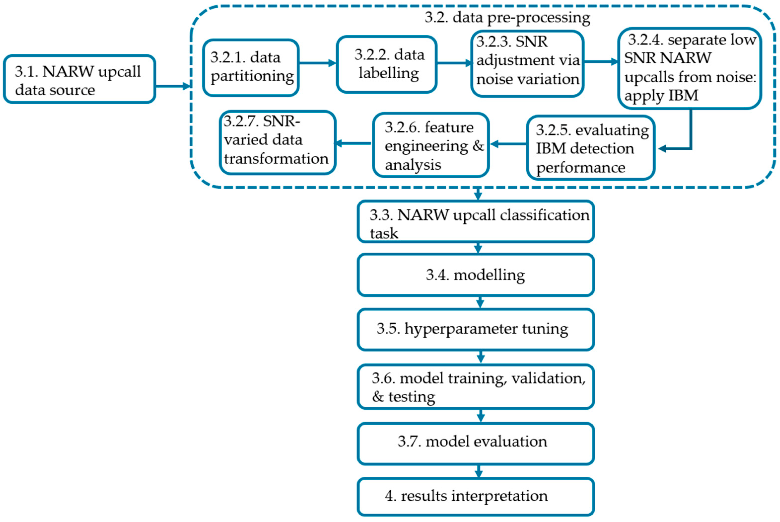
Figure 1. Methodological pipeline including data pre-processing (Section 3.2); NARW upcall classification task (Section 3.3); modeling (Section 3.4); hyperparameter tuning (Section 3.5); model training, validation, and testing (Section 3.6); model evaluation (Section 3.7); and results interpretation (Section 4). The workflow starts in the upper left corner (Section 3.1). The numbers in each box indicate the section of the paper where that topic is discussed.
Make 07 00154 g001
Figure 2. Geographic location of recording sites for the DCLDE NARW upcalls in the Gulf of Maine, off the coast of Massachusetts. The red circles indicate the precise locations of the Cornell University MARU hydrophone deployment sites (A–F). These recorders formed a fixed array used for data collection from 2000 to 2009. The precise coordinates (World Geodetic System of 1984 (WGS84)) for each site are listed in the adjacent table.
Make 07 00154 g002
Figure 3. Workflow process to generate the designed noise n ( t ) to achieve the S N R d (Equation (1)) for each v t . P S + n is the power of the noise reduced from v ( t ) , discretized in time as v i , and μ is the mean of the noise segment, n s e g ,   for a particular v t . P d is the desired noise power to achieve a specific S N R d and n t is the background noise. Note that the length of the noise array is equal to the length of the upcall v t .
Make 07 00154 g003
Figure 4. Time–frequency (spectrogram) representations of (a) v(t) as in the dashed white box; (b) noise n(t) as in Equation (3); and (c) X ( t , f ) as in the dashed white box (Equation (4)).
Make 07 00154 g004
Figure 5. IBM applied to a superposed signal containing an upcall vocalization and background noise. The mask is created by comparing the energy of the target upcall signal to the energy of the noise in each time–frequency bin by assigning 0 to pixels below the signal threshold and 1 to those above the threshold. White pixels represent time–frequency bins where the upcall energy is higher than the noise is assigned, and black pixels represent bins where the noise energy is higher than the upcall.
Make 07 00154 g005
Figure 6. Example distributions (solid blue line) for 6 of the 20 extracted features (Table 4) across all curated upcalls (81,567): (a) energy_rms ( V 2   ); (b) mfcc_mean; (c) mag_spec_mean; (d) energy_var ( V 2 ); (e) mfcc_var; and (f) mag_spec_var. Features (ae) exhibit right skew, while (f) shows a normal left-skewed distribution. Understanding these patterns allows for appropriate re-scaling to minimize skew and potential bias. Robust scaler normalization will be used.
Make 07 00154 g006
Figure 7. Example checks for outliers in 6 of the 20 extracted feature types (blue boxes represent feature IQR and small circles indicate the outliers): (a) energy_rms ( V ); (b) mfcc_mean; (c) mag_spec_mean; (d) energy_var ( V 2 ); (e) mfcc_var; and (f) mag_spec_var. The energy_rms feature (a) has outliers, while (be) does not. Although outliers within features are typically removed, they were retained as the upcalls have rich spectra that span a large range and thus may not be true outliers.
Make 07 00154 g007
Figure 8. Correlation analysis to show the strength of the relationships between the feature types of the SNR-varied acoustic dataset. Values   0.70   or     0.70   are classified as strong negative and positive correlations, respectively, as analyzed in Table A2. Some of the features have weak correlations but are retained because they contain important inferred information about other random variables, and therefore they are jointly associated with it.
Make 07 00154 g008
Figure 9. SNR-varied data distribution after applying the robust scaler method. Robust scaler normalization helps mitigate slower convergence by ensuring that features are on a similar scale, to handle outliers. This stability during the training iterations reduces the adverse impact on classification results by enabling the IBM-BHN method to learn more effectively.
Make 07 00154 g009
Figure 10. A workflow diagram of the proposed IBM-BHN pipeline.
Make 07 00154 g010
Figure 11. The architecture of the proposed IBM-BHN method, illustrating how the SNR-varied acoustic data are processed. IBM-BHN has proven sensitive to low-SNR NARW upcalls.
Make 07 00154 g011
Figure 12. Information flow in an LSTM cell through input i m , forget f m , output ( o m ) , and hidden ( h m ) gates.
Make 07 00154 g012
Figure 13. Highway network architecture showing information flow across the layers of the BiLSTM method.
Make 07 00154 g013
Figure 14. Learning curves depicting training and validation loss trajectories over time. The training loss curve shows a consistent downward trend, demonstrating that the model progressively minimized its error on the training set. The narrow and stable gap between the two curves throughout all 50 epochs confirms that the implemented regularization techniques—dropout (rate = 0.5) and L2 regularization ( λ   = 0.001)—were effective in mitigating overfitting. This behavior underscores the robustness of the proposed model and its suitability for deployment.
Make 07 00154 g014
Figure 15. ROC curves showing the proposed IBM-BHN model effectively learned the SNR-varied upcalls, despite the upcall’s complex time, frequency, and cepstral properties. The AUC quantifies the model’s ability to distinguish between upcall vocalization (class 1) and noise (class 0), where higher AUC is better. The proposed highway–BiLSTM achieved an AUC of 0.99, which is superior to all baseline methods considered.
Make 07 00154 g015
Figure 16. IBM-BHN and baseline models performance comparison based on all classes (12,303 positive and 12,303 negative test samples): (a) SVM demonstrates high sensitivity in correctly classifying noise (near-50%). However, its correct upcall classification is relatively low (17%). In contrast, ANN (b) and CNN (c) exhibit good upcall classification (32% and 39%, respectively) with also high noise classification (near-50% and 46%, respectively). ResNet (d) offers moderate correct classification, with 44% for upcall and 50% for noise. LSTM (e) shows high upcall sensitivity (39%), but its noise classification drops to 44%. Lastly, IBM-BHN (f) demonstrates high sensitivity in correctly classifying noise (49%, similar to SVM) and upcalls (50%). IBM_BHN is a robust model to distinguish upcalls and noise.
Make 07 00154 g016aMake 07 00154 g016b
Table 1. Summary of existing detection and classification studies, highlighting methodological diversity and the absence of quantitative performance evaluations in low-SNR conditions or network optimization strategies.
Ref.ClassifierDatasetFeature Extraction AccuracyNetwork OptimizationSNR Ranges (dB)
[19]SVMDCLDEMFCC & DWT92%NoNot specified
[20]ANNPAM deployed at Stellwagen Bank National Marine Sanctuary.Spectrogram and human perception features.86%NoSNR > 0 dB
[21]MLPPAM deployed at St. Lawrence River Estuary.Short-time Fourier transform (STFT) and wavelet packet transform (WPT).86%NoNot specified
[23]CNNKaggleMel-filter bank (mel-spectrograms)84%NoNot specified
[24]CNNPAM deployed at Bay of Fundy.Spectrogram95%NoNot specified
[25]ResNetDCLDESpectrogramRecall of 80% and precision of 90%.NoSNR > 0 dB
[26]LeNetPAM deployed in New Zealand waters.Spectrogram96%NoSNR > 0 dB
[27]LSTMSelf-collected dataset.Spectrogram98%NoNot specified
[29]Swin TransformerWatkins Marine Mammal Sound DatabaseSpectrogram and phase-related features.95%NoNot specified
[30]Self-supervised learning and ASTAudioSet and ESC-50SpectrogramAn average improvement
of 60.9%.
NoNot specified
[31]Transformer-Based Few-ShotDCASE 2022 task-5Spectrogram73%NoNot specified
Proposed IBM-BHNDCLDE20 acoustic features across time, frequency, and cepstral domains Yes−10 dB to 10 dB
Table 2. Summary of NARW vocalization data extracted from the DCLDE 2013 repository.
CategoryValueDescription
Total audio files67215 min long files
Total recording duration168 h672 files ×   15   60   ( m i n )
Total NARW upcalls9063Extracted from annotated files, approximately 3 s each.
Background noise samples67215 min long files
SNR range 0.10   dB to 5   dB Before noise addition
Table 3. Pseudo-code for ideal binary mask separation. This was used to investigate the lowest SNR where NARW upcall detection is possible. Additionally, it was used to separate the desired signal (e.g., upcall) and noise. The outputs of this separation are the recovered time domain upcall ( v r ( t ) ) and the noise ( n r ( t ) ). Separate low-SNR NARW upcalls from noise using IBM.
Algorithm 1: Separate Low SNR NARW Upcalls from Noise using IBM
1: initialize: prepare signal x ( t )
2: apply STFT to x ( t ) to obtain its t f representation
3: for each t f bin do Equation (5)
4:   if  X i j t , f > t h then w = 1
5:     else
6:         w = 0
7:   end if
8:  end
9:  apply binary mask w ( t , f ) to X ( t , f ) Equation (6)
10: apply inverse STFT to Equation (6)
11: output:  v r ( t ) and noise n r ( t )
Table 4. Comparison of the computation time for NARW upcall separation using the IBM versus the manual method. The manual method is based on linear scaling. The IBM method computation time is calculated using Equation (7). Lower computation time indicates higher efficiency. This comparison highlights the IBM method’s superior efficiency.
No. of Audio Recording
(3 s Duration)
Manual Method (s)Proposed IBM Method (s)
10 ~   6000.05
20 ~   12000.08
30 ~   18000.13
40 ~   24000.17
50 ~   30000.18
Table 5. Proposed IBM method’s performance on vocalization detection over a range of S N R : (a) original or raw upcall v t ; (b) IBM recovered upcall v r t ; (c) correlation between the original or raw (a) and IBM recovered upcalls (b); (d) difference between raw and recovered upcalls; (e) superposed signal; and (f) correlation between the original and superposed signals. The relatively high correlations (c) even for S N R < 0 suggest that the IBM is a good method to extract acoustic signals from low S N R environments.
S N R dB
(Equation (1))
(a) Original Signal
v t
(b) IBM Recovered
Signal   v r t
(Table 1)
(c) Correlate
r a , b
(Equation (8))
(d) Difference of
(a)–(b)
v t v r t
( e )   Superposed   Signal   x t (Equation (3))(f) Correlate
r ( a , ( e ) )
(Equation (8))
10Make 07 00154 i001Make 07 00154 i0020.95Make 07 00154 i003Make 07 00154 i0040.58
8Make 07 00154 i005Make 07 00154 i0060.94Make 07 00154 i007Make 07 00154 i0080.50
6Make 07 00154 i009Make 07 00154 i0100.93Make 07 00154 i011Make 07 00154 i0120.43
3Make 07 00154 i013Make 07 00154 i0140.91Make 07 00154 i015Make 07 00154 i0160.34
0Make 07 00154 i017Make 07 00154 i0180.90Make 07 00154 i019Make 07 00154 i0200.26
−3Make 07 00154 i021Make 07 00154 i0220.87Make 07 00154 i023Make 07 00154 i0240.21
−6Make 07 00154 i025Make 07 00154 i0260.85Make 07 00154 i027Make 07 00154 i0280.17
−8Make 07 00154 i029Make 07 00154 i0300.83Make 07 00154 i031Make 07 00154 i0320.15
−10Make 07 00154 i033Make 07 00154 i0340.13Make 07 00154 i035Make 07 00154 i0360.13
Table 6. Proposed IBM-BHN algorithm for the NARW upcall classification. Operation of the proposed IBM-BHN classifier.
Algorithm 2: Operation of the Proposed IBM-BHN Classifier
Require: Given the input sequence as X m = { x 1 , x 2 , x 3 , …, x N }, y m   ∈ {0, 1}
1:  use BiLSTM to capture contextual information
2:  use Equations (11)–(14) to obtain the feature representation
3:  feed the output of step 2 into a highway layer
4:  flatten the output of step 3
5:  input flattened features into the dense layer with L2
   regularization rate
6:  pass the output of step 5 into a dropout layer
7:  specify p
8:  pass step 7 into the fully connected layer
9:  perform classification using a sigmoid activation function
10: apply binary cross-entropy loss
11: use Adam optimization 
12: update the weights and biases of the proposed method
Table 7. Hyperparameter values used to tune the proposed IBM-BHN and five baseline methods.
ModelHyperparameterValueOptimal
SVM
regularization parameter (C)
0.1, 1, 10, 100
0.1
kernel
linear, polynomial, and radial basis function, sigmoid
polynomial
ANN
unit
16, 32, 64, and 96
32
learning rate
10 3 ,   10 4 ,   10 5 ,   10 6 ,   2 × 10 5
10 6
optimizer
Adam and SGD
Adam
dropout
0.1, 0.2, 0.3, 0.4, and 0.5
0.5
epoch
50, 100 and 150
50
batch size
16, 32, 64, and 96
96
number of layer
   __2 (1 hidden dense,
1 output dense)
activation function
ReLU, Tanh
hidden: ReLU
output: Sigmoid
CNN
filter
16, 32, 64, and 96
16
kernel size
1, 2, 3, 4
1
learning rate
10 3 ,   10 4 ,   10 5 ,   10 6 ,   2 × 10 5
10 6
optimizer
Adam and SGD
Adam
dropout
0.1, 0.2, 0.3, 0.4, and 0.5
0.1
epoch
50, 100, 150
50
batch size
16, 32, 64, and 96
96
number of layer
   __2 (1 Conv1D, 1 output dense)
activation function
ReLU, Tanh
hidden: ReLU
output: Sigmoid
ResNet
filter
16, 32, 64, and 96
16
kernel size
1, 2, 3, 4
1
learning rate
10 3 ,   10 4 ,   10 5 ,   10 6 ,   10 7 ,   2 × 10 5
10 7
optimizer
Adam and SGD
Adam
dropout
0.1, 0.2, 0.3, 0.4, and 0.5
0.1
epoch
50, 100, 150
50
batch size
16, 32, 64, and 96
96
number of layer
   __8 (7 Conv1D,
1 output dense)
activation function
ReLU, Tanh
hidden: ReLU
output: Sigmoid
LSTM
unit
16, 32, 64, and 96,
32
learning rate
10 3 ,   10 4 ,   10 5 ,   10 6 ,   2 × 10 5
10 5
optimizer
Adam and SGD
Adam
dropout
0.1, 0.2, 0.3, 0.4, and 0.5
0.5
epoch
50, 100, 150
50
batch size
16, 32, 64, and 96
64
number of layer
   __3 (1 LSTM, 1 dense, 1 output dense)
activation function
ReLU, Tanh
hidden: Tanh
output: Sigmoid
IBM-BHN
unit
16, 32, 64, and 96,
16
learning rate
10 3 ,   10 4 ,   10 5 ,   10 6 ,   2 × 10 5
10 6
optimizer
Adam and SGD
Adam
dropout
L2 regularization
0.1, 0.2, 0.3, 0.4, and 0.5
  10 2 ,   10 3 ,   10 4 ,   10 5 ,  
0.5
10 3 ,
epoch
50, 100, 150
50
batch size
16, 32, 64, and 96
96
number of layer
   __3 (1 BiLSTM, 1 highway, 1 output dense)
activation function
ReLU, Tanh
hidden: Tanh
output: Sigmoid
Table 8. 2 × 2 contingency table for McNemar’s test.
Misclassified by Both Models
(Proposed and Baseline): n 00
Misclassified by Proposed IBM-BHN Model Only: n 01
misclassified by baseline only: n 10 correctly classified by both models (proposed baseline): n 11
Table 9. Performance comparison of the proposed IBM-BHN and baseline models on the test dataset of sample size 24,606 audio recordings (12,303 positive and 12,303 negative instances). Evaluating the IBM-BHN model on a separate dataset ensures its performance is not confined to the training data and thus generalizes well to unseen data. IBM-BHM outperforms most baseline models across most metrics, and the Δ columns show the IBM-BHN’s improvement over the baseline models considered.
ModelAccuracyPrecisionSensitivity F1-Score
Actual (%) Δ Actual (%) Δ Actual (%) Δ Actual (%) Δ
SVM6731603999−37523
ANN8216732699−38513
CNN851380199338612
ResNet94490999−3944
LSTM831580198798315
IBM-BHN980990960980
Table 10. Results of McNemar’s chi-square test comparing the proposed IBM-BHN model against baseline classifiers (SVM, ANN, CNN, ResNet, and LSTM) on the test set N = 24,606 . Reported values include the chi-square statistic with 1 degree of freedom, p-value, and   ψ .
Comparison χ 2 ( 1 , N = 24,606 ) p-Value ψ
BiLSTM vs. SVM 2.70 × 10 8 < 0.001 0.94
BiLSTM vs. ANN 6.44 × 10 3 < 0.001 0.85
BiLSTM vs. CNN 2.84 × 10 3 < 0.001 0.75
BiLSTM vs. ResNet 2.70 × 10 8 < 0.001 0.94
BiLSTM vs. LSTM 2.69 × 10 8 < 0.001 0.94
Table 11. Comparison of false positive and negative rates for IBM-BHN and the baseline models considered. SVM, ANN, CNN, ResNet, and LSTM have a higher false positive than false negative rate, while the IBM-BHN method shows no false positives and a low false negative rate. This suggests IBM-BHN is effective, making it a strong candidate for classifying NARW upcalls.
ModelFalse Positive Rate (%) False Negative Rate (%)
SVM400.1
ANN270.1
CNN208
ResNet101
LSTM2014
IBM-BHN0.11
Table 12. Computation performance comparison of the proposed IBM-BHN model and baseline models. The IBM-BHN model demonstrates a faster response time than the ResNet. Faster response time implies that the IBM-BHN model can quickly classify the NARW upcall from noise, making it more efficient and suitable for real-time applications.
ModelTraining Time (s)Response Time (s)
ANN30.16
CNN40.19
ResNet670.48
LSTM110.20
IBM-BHN130.12
Table 13. Impact of BiLSTM units on the proposed IBM-BHN classifier. The number of units does not have a substantial effect on model performance.
BiLSTM CellsPrecisionSensitivity
969996
649996
329996
169996
Table 14. Comparison of false positive and false negative rates to assess the impact of imbalanced evaluation test dataset on the performance of the proposed IBM-BHN and baseline models. Despite the imbalanced test dataset, IBM-BHN still has reduced false alarms and reliably classifies upcalls.
ModelFalse Positive Rate (%) False Negative Rate (%)
SVM860
ANN670
CNN2313
ResNet76
LSTM1416
IBM-BHN60
Table 15. Comparison of false positive and false negative rates to assess the impact of different SNR evaluation test datasets on the models’ performance.
SNR (dB)False Positive Rate (%) False Negative Rate
(%)
1000
800
600
300.1
000.4
−30.10.9
−60.21.6
−80.22.6
−100.54.3
Table 16. Comparison of the IBM-BHN classifier’s core metrics (accuracy and F1-score) against the best-performing baseline model for NARW upcall classification.
MetricIBM-BHN Score
(%)
Best Baseline Score
(ResNet) (%)
Improvement Over Baseline (%)
accuracy98.094.04.3
F1-score98.094.04.3
Disclaimer/Publisher’s Note: The statements, opinions and data contained in all publications are solely those of the individual author(s) and contributor(s) and not of MDPI and/or the editor(s). MDPI and/or the editor(s) disclaim responsibility for any injury to people or property resulting from any ideas, methods, instructions or products referred to in the content.