A Comprehensive Study on Short-Term Oil Price Forecasting Using Econometric and Machine Learning Techniques

Abstract

This paper investigates the short-term predictability of daily crude oil price movements by employing a multi-method analytical framework that incorporates both econometric and machine learning techniques. Utilizing a dataset of 21 financial and commodity time series spanning ten years of trading days (2015–2024), we explore the dynamics of oil price volatility and its key determinants. In the forecasting phase, we applied seven models. The meta-learner model, which consists of three base learners (Random Forest, gradient boosting, and support vector regression), achieved the highest R² value of 0.532, providing evidence that our complex model structure can successfully outperform existing approaches. This ensemble demonstrated that the most influential predictors of next-day oil prices are VIX, OVX, and MOVE (volatility indices for equities, oil, and bonds, respectively), and lagged oil returns. The results underscore the critical role of volatility spillovers and nonlinear dependencies in forecasting oil returns and suggest future directions for integrating macroeconomic signals and advanced volatility models. Moreover, we show that combining multiple machine learning procedures into a single meta-model yields superior predictive performance.

1. Introduction

Crude oil lies at the heart of the global economy, fueling factories, automobiles, and power stations; consequently, when its price fluctuates, investors, corporations, and central banks all feel the impact. Even small price movements can ripple through financial markets, prompting portfolio managers and policymakers to seek reliable forecasts of oil prices over the coming days or weeks. Recent research tackles this forecasting challenge along three main fronts. Haung et al. [1], Alkhammash [2] and Al-Fattah [3] employ gradient boosting algorithms and deep neural networks to capture the nonlinear patterns in oil’s movements. Second, hybrid “decompose-and-learn” methods [4,5,6,7,8] first decompose the raw price series into smoother, wave-like components via EEMD or CEEMDAN, then feed these components into models ranging from sparse Bayesian learners to Hidden Markov regressions. Third, enhanced classical frameworks remain relevant: ARIMA-GARCH models [9,10,11] refine linear autoregressive structures, while spillover analyses [12,13] examine how oil shocks propagate into equity markets; Figuerola-Ferretti et al. [14] further show that analyst sentiment and expert bias can be as informative as historical price data. Traditional models, however, often struggle to integrate external market forces and sharp nonlinearities. In response, researchers increasingly rely on robust algorithms such as Random Forests, gradient boosting, and support vector regression. In the present study, we combine these three methods within a stacked meta-learning model allowing each learner to leverage its strengths before blending their predictions and enrich our dataset with 21 market variables, including volatility indices (VIX, OVX, and MOVE), interest rates, and major commodity returns, so the model can capture the broader financial context rather than merely extrapolating from past oil price movements. The major contribution of this paper is the development and empirical validation of this novel meta-learning framework, which achieves an out-of-sample RMSE of 2.04, MAE of 1.65, and test-set R² of 0.532, outperforming all individual models and demonstrating that VIX, OVX, MOVE, and lagged oil returns are the principal drivers of next-day oil-price dynamics, offering both methodological innovation and practical guidance for market participants and academics.

2. Literature Review

Given oil’s central role in the global economy, it is no surprise that scholars have tried a wide range of approaches to better understand and predict its price movements, from classic statistical models to more modern machine learning tools. Alquist and Kilian [15] examined whether futures prices could reliably predict oil price movements. They found that, while futures offer some short-term signals, their usefulness as long-range predictors is limited. This spurred the development of more advanced time-series methods, especially those focused on modeling volatility. Among the most widely used tools in this space are GARCH models [16,17]. Fu [17] proposed a GARCH-LSTM framework that captures conditional heteroskedasticity while leveraging deep sequence learning, outperforming traditional GARCH and pure LSTM models. Similarly, Zhang and Zhang [16] incorporated structural break detection into a GARCH-based forecasting model, demonstrating that accounting for regime shifts significantly improves price prediction accuracy during geopolitical and macroeconomic disruptions. Li et al. [18] integrated CEEMDAN with hierarchical multi-resolution regression (HMR), showing that decomposition followed by targeted regression layers can better isolate price signal components.

Stochastic models have also gained ground. Mwanakatwe, Daniel, and Nzungu [19] applied the Heston model to oil price volatility and found that it captured certain features of the data, like long memory and sharp jumps, better than traditional models. These results support the idea that models allowing for random volatility changes can better reflect real market behavior. A large body of work has explored how oil prices interact with other parts of the financial system. Refs. [20,21,22,23] suggested that oil does not move in isolation and information from broader financial markets can offer useful clues for predicting price changes. Balcilar et al. [24] discovered that oil price uncertainty has a stronger effect on bond market volatility than on bond returns. Qin [25] introduced a spillover-based forecasting framework using OVX, WTI, and Brent volatility interactions, highlighting the predictive value of implied volatility indices and cross-market uncertainty. Qin and Bai [26] showed that realized volatility in oil prices can help predict future stock market swings. Dutta [27] found that oil market uncertainty has asymmetric effects on U.S. biofuel companies, highlighting the wider economic influence of crude oil volatility. Safari and Davallou [28] used a combination of models, including the exponential smoothing model (ESM), autoregressive integrated moving average model (ARIMA), and nonlinear autoregressive (NAR) neural network, to increase the accuracy of forecasting crude oil prices. Abdollahi [29] also proposed a hybrid model for oil price forecasting. He combined support vector machine, particle swarm optimization, and Markov-switching generalized autoregressive model and demonstrated that the proposed model outperforms other models. Yang et al. [30] combined traditional economic data and Google Search Volume Index (GSVI) reflecting macro and micro mechanisms affecting crude oil price. Their hybrid model included K-means clustering, Kernel Principal Component Analysis (KPCA), and Kernel Extreme Learning Machine (KELM). The “divide and conquer” strategy used in their study achieved a better forecasting performance.

The recent literature on oil short-term price forecasting has shifted from traditional econometric models toward sophisticated hybrid architectures that combine signal decomposition techniques with advanced machine learning approaches to address the inherent volatility and non-stationarity of oil markets. Contemporary research demonstrates that decomposition-based hybrid models, particularly those integrating variational mode decomposition (VMD) or Local Mean Decomposition (LMD) with deep learning architectures such as LSTM, consistently outperform traditional ARIMA and SARIMA models in terms of MAE, MAPE, and RMSE metrics [31,32,33]. Peng et al. [34] proposed a forecasting framework that incorporates variational mode decomposition (VMD), time-series imaging, and a bidirectional gated recurrent unit network (BGRU). Their results demonstrate that all three models constructed following our approach outperform benchmark methods. Specifically, our VMD-RP-BGRU model achieves the best forecasting performance.

Foroutan and Lahmiri [35] used 16 deep and machine learning models to forecast the daily price of the West Texas Intermediate (WTI), Brent, gold, and silver markets. They integrated Temporal Convolutional Networks (TCNs) and attention-augmented LSTMs for capturing long-range dependencies in price movements. Their results reveal that the TCN model outperforms the others for WTI, Brent, and silver, achieving the lowest MAE values of 1.444, 1.295, and 0.346, respectively. Kumar [36] presented a reservoir computing (RC) model specifically designed for precise crude oil price predictions, outperforming traditional methods such as ARIMA, LSTM, and GRU. Results demonstrated that during periods of economic disruption, such as the COVID-19 lockdowns, the RC model effectively captured sharp price fluctuations, highlighting its robust forecasting capability.

Alruqimi and Di Persio [37] introduced a Conditional GAN (CO-CGAN), a hybrid model for enhancing crude oil price forecasting by combining advanced AI frameworks (GANs), oil market sentiment analysis, and stochastic jump-diffusion models. Their offered model integrates a Lévy process and sentiment features to better account for uncertainties and price shocks in the crude oil market. Other researchers combined gradient-boosted trees (XGBoost and LightGBM) with neural networks and error-correction modules, demonstrating superior performance in multi-stage forecasting pipelines. The empirical evidence consistently shows that hybrid approaches leveraging decomposition preprocessing, specialized modeling of different frequency components, and ensemble/correction stages achieve 15–30% improvements in forecasting accuracy over single-model baselines, particularly during volatile market conditions and crisis periods such as the COVID-19 pandemic and geopolitical disruptions [38,39].

The meta-learner developed in this study differs substantially from the deep and hybrid forecasting architectures reported in the referenced literature. Recent approaches such as Transformer snapshot ensembles [40] and dual-attention [37] rely on deep sequential parameterization to automatically extract temporal dependencies and hierarchical feature representations, often coupled with large training windows and high computational cost. Similarly, hybrid decomposition models like CEEMD-ARIMA-SSA-BP [41], ICEEMDAN-based pipelines, and reservoir computing frameworks [36] apply multi-stage architectures with preprocessing, subseries modeling, or recurrent dynamics to enhance nonlinear signal capture. Blending models [42,43] and shrinkage approaches embedded in extended HAR structures [44] also involve either heterogeneous learner fusion or penalized regression over expanded variable sets. In contrast, the meta-learner model follows a two-level stacked architecture. In the first stage, Random Forest, gradient boosting, and SVR independently generate forecasts. Their predictions are then used as inputs to a second-stage gradient boosting regressor, which learns how to combine them.

The literature also identifies critical gaps, including inconsistent evaluation protocols across studies, limited focus on probabilistic forecasting and uncertainty quantification, insufficient validation across different market regimes, and the need for standardized benchmarking frameworks that can reliably compare hybrid methodologies. This study contributes to the literature by applying a meta-learning approach across a broad panel of predictors spanning 2015–2024, integrating economic, financial, and volatility-based variables. By benchmarking multiple machine learning models, including tree-based ensembles, deep learners, and regularized regression techniques, and combining their predictions, the analysis demonstrates substantially higher explanatory power than most prior studies. The extended time window and multi-class learning architecture address limitations in both recency and methodological breadth identified in the existing literature.

3. Data and Methodologies

The data for this study consists of ten years of daily observations covering the period from 1 January 2015 to 31 December 2024. We used 21 time series encompassing oil price daily returns, volatility indexes (Equity—VIX, Oil—OVX, and Bonds—MOVE), yields (3-year and 10-year U.S. Treasury yields), spreads (the gaps between the yields of 3 and 10 years government bonds), a broad range of commodity returns (Gold, Silver, Copper, Iron, Aluminum, Coffee, Corn, Wheat, Sugar, Rice, Meat, and Orange), and two equity indexes (the S&P 500 and EURO STOXX 50). Our analysis began with a stepwise multiple regression (Model 1) to identify the explanatory variables of oil price movements, and Model 2, an autoregressive (AR) model, was used to capture short-term momentum in daily oil returns.

$$Oi{l}_t={\beta }_0+{\beta }_n{X}_t+{\epsilon }_t$$

(1)

where $X_t$ is an explanatory variable at time t, and n is the number of variables left after the stepwise procedure.

$$Oi{l}_t={\varnothing }_0+{\varnothing }_{1}Oi{l}_{t-1}+{\epsilon }_t$$

(2)

To capture time-varying volatility (volatility clustering) in oil returns, we utilized ARCH(1) Model 3:

$${\sigma }_t^2={\alpha }_0+{\alpha }_1{\epsilon }_{t-1}^2+{\mu }_t$$

(3)

In addition, we utilized Principal Component Analysis (PCA) as a dimensionality-reduction technique that transforms a possibly large set of correlated variables into a smaller set of uncorrelated variables called principal components (PCs). Finally, to deepen our understanding of the factors influencing oil prices, we constructed seven prediction models: Random Forest, gradient boosting, support vector regression (SVR), ARIMA, ARIMAX, Error Trend Seasonality (ETS), and LassoCV.

3.1. Model Specifications

All machine learning models were implemented using default parameter settings provided by the respective libraries, and no manual hyperparameter tuning was conducted, except for the automatic selection of the regularization parameter λ in LassoCV. This design choice prioritizes reproducibility and reflects real-world forecasting settings where extensive tuning is often impractical. The Random Forest model was implemented using default parameters. Specifically, 100 decision trees were constructed, each trained using bootstrap sampling with no restriction on maximum tree depth. The Gini impurity criterion was used to determine split quality, and nodes were allowed to expand until leaves were pure or contained fewer than two samples. These defaults provide robust performance in noisy financial contexts without overfitting. The gradient boosting model followed the standard configuration, consisting of 100 boosting stages with a learning rate of 0.1. Each weak learner was a decision tree with a maximum depth of three. The squared error loss function was used, and the subsample parameter remained at its default value of 1.0, meaning all samples were used for each boosting iteration. This setup captures nonlinear relationships effectively without requiring manual tuning. The SVR model was applied with its default settings. The radial basis function (RBF) kernel was used to model nonlinearities, with the regularization parameter C = 1.0 and an epsilon margin of 0.1 defining the tolerance for prediction errors. The gamma parameter followed the default “scale” heuristic, which automatically adjusts kernel sensitivity based on the input data distribution. Lasso regression with cross-validation was employed using default parameters. The model performed five-fold cross-validation to automatically select the optimal regularization parameter λ. The coordinate descent algorithm was used for optimization, and standard preprocessing assumptions from the library were applied. This approach enabled implicit feature selection by shrinking less relevant predictor coefficients toward zero. The ARIMA model was fitted using the default behavior of the statistical package, which selects the autoregressive (p), differencing (d), and moving average (q) terms based on information criteria and stationarity diagnostics. No seasonal components were specified. Maximum likelihood estimation was used to fit the parameters, allowing the model to serve as a classical baseline for comparison. The ARIMAX model extended ARIMA by including exogenous predictors while maintaining the same automatic selection of p, d, and q. The statistical software inferred the appropriate lag order and used maximum likelihood estimation for parameter fitting. The inclusion of external variables provided a hybrid perspective that combined time dependence with additional explanatory signals. Finally, the ETS model was estimated by using default settings, allowing the software to automatically determine the presence of error, trend, and seasonal components. No manual smoothing parameters were specified. This configuration allowed the model to adaptively decompose level and trend dynamics without imposing predefined structure.

3.2. The Meta-Learner Model

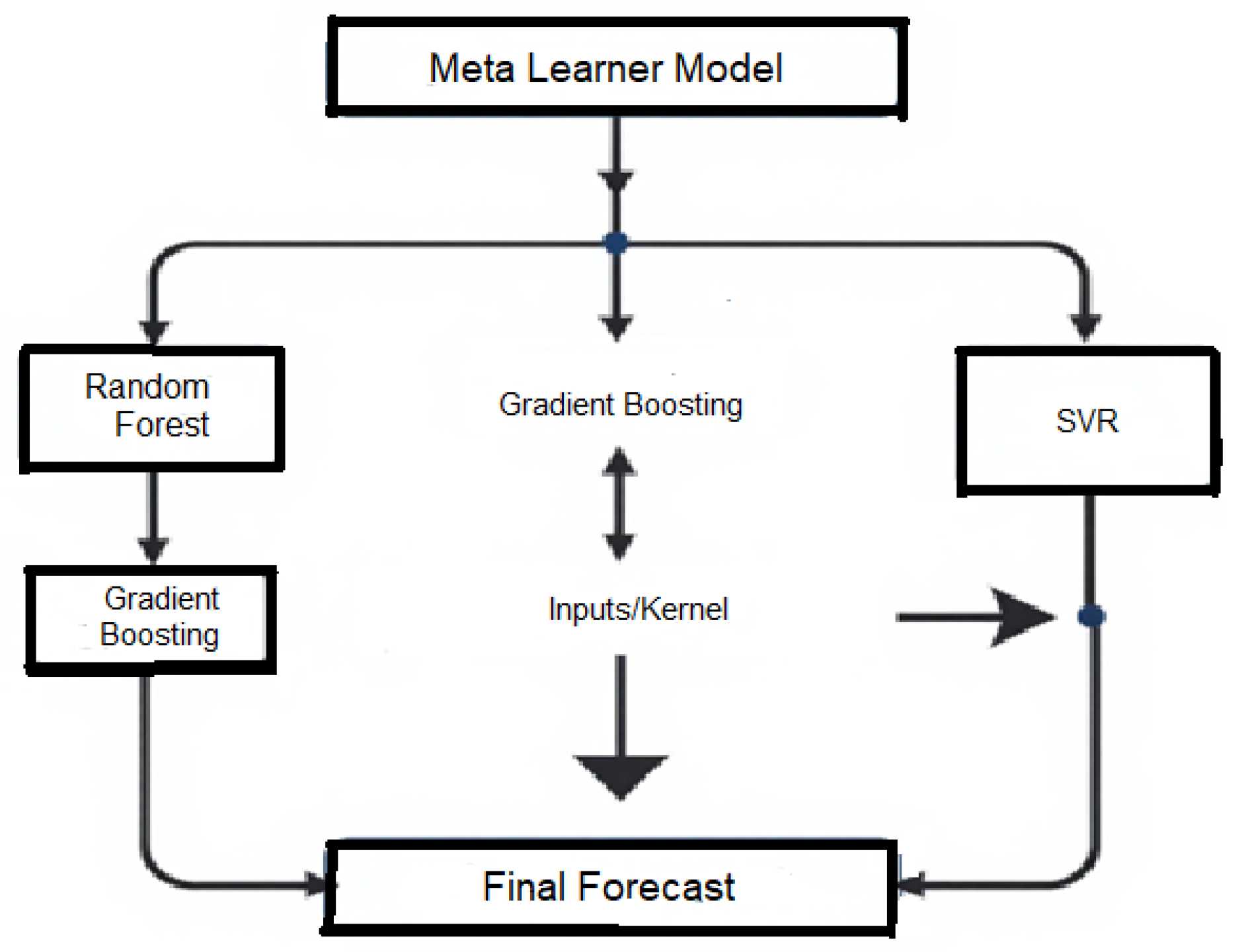
After evaluating the performance of all individual models, the three best-performing algorithms were combined into a stacked ensemble. In the first stage, Random Forest, gradient boosting, and SVR independently generated forecasts. These first-level predictions were then used as inputs to a second-stage gradient boosting regressor, which learned how to combine them. This architecture reduces idiosyncratic model risk and exploits the complementary strengths of the base learners. Random Forest captures nonlinearities and provides variable importance, gradient boosting models interactions, and SVR is robust to noisy, high-variance data. The stacked structure preserves the strengths of the individual models while reducing variance and improving overall predictive performance. Unlike deep learning models such as LSTM, GRU, or CNN-based architectures, which rely on hierarchical feature extraction from long sequential inputs, the meta-learner model combines the outputs of the three best-performing traditional models through a second-stage gradient boosting regressor, which learns how to combine them.

Deep learning models typically learn temporal dependencies end-to-end using recurrent or convolutional layers and require large volumes of high-frequency data to generalize effectively. In contrast, the meta-learner model operates on engineered features derived from fundamentals, technical indicators, and entropy-based signals, allowing each base model to capture distinct predictive structures without excessive parameterization. The combined design improves robustness by reducing variance across individual models while avoiding overfitting risks commonly associated with deep learning architectures trained on limited daily financial datasets. Moreover, this structure maintains model interpretability and computational efficiency, which are often compromised in deep neural networks that involve thousands or millions of parameters.

The model uses 21 time series which are preprocessed through standardization and kernel transformations where necessary, before being passed into three base learners: (1) Random Forest, which builds multiple decision trees on bootstrapped samples to capture nonlinear effects and provide feature importance; (2) gradient boosting, which sequentially builds trees that correct the errors of previous ones to model complex interactions; and (3) support vector regression, which employs kernel functions such as the RBF kernel to capture nonlinearities while controlling complexity. The predictions from these three learners are then treated as new features for a gradient boosting regressor serving as the meta-learner, which has been trained (using careful cross-validation so it never cheats by seeing the answers ahead of time) to learn when to trust, down-weight, or creatively combine the others. The training period included five years of daily returns and a quarterly rolling re-training period to adapt to market structure changes.

The model mixes in extra kernel-tweaked versions of the original inputs so it can deliver one well-balanced final forecast that is more accurate than any single model on its own. The final forecast, produced by this stacked ensemble, effectively reduces variance through Random Forest, minimizes bias through gradient boosting, and captures nonlinear dependencies through SVR, thereby leveraging the complementary strengths of the three methods for robust oil price forecasting.

All computational experiments were carried out using Python 3.11 on a desktop computer. Machine learning algorithms, including Random Forest, gradient boosting, support vector regression, and the stacked meta-learner, were implemented using the scikit-learn 1.4 library. Econometric models (ARIMA, ARCH, and ETS) were estimated using the statsmodels package, while pandas 2.2 and matplotlib 3.8 were employed for data handling and visualization. Random seeds were fixed to enhance reproducibility. The full structure of the meta-learner model can be found in Figure 1.

4. Results

We start by exploring the parts of the data using Figure 2 and Figure 3.

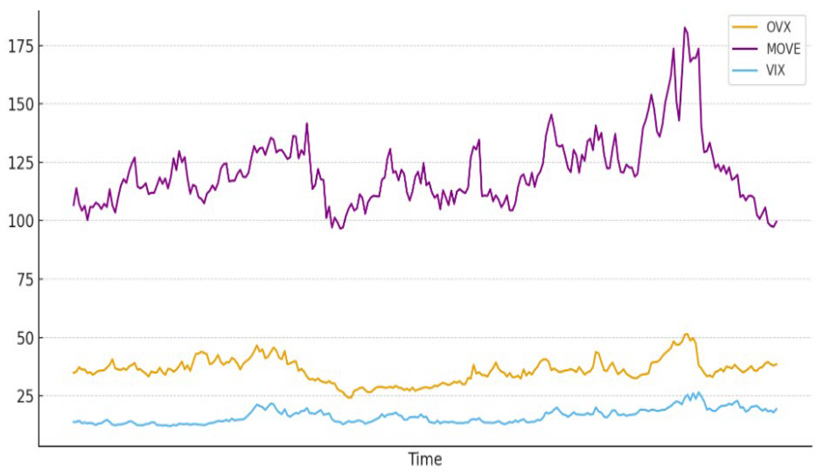
In Figure 4, we can see that the oil volatility (OVX) index in 2023–2024 lies between S&P500 Volatility (VIX) and U.S Bonds volatility (Move).

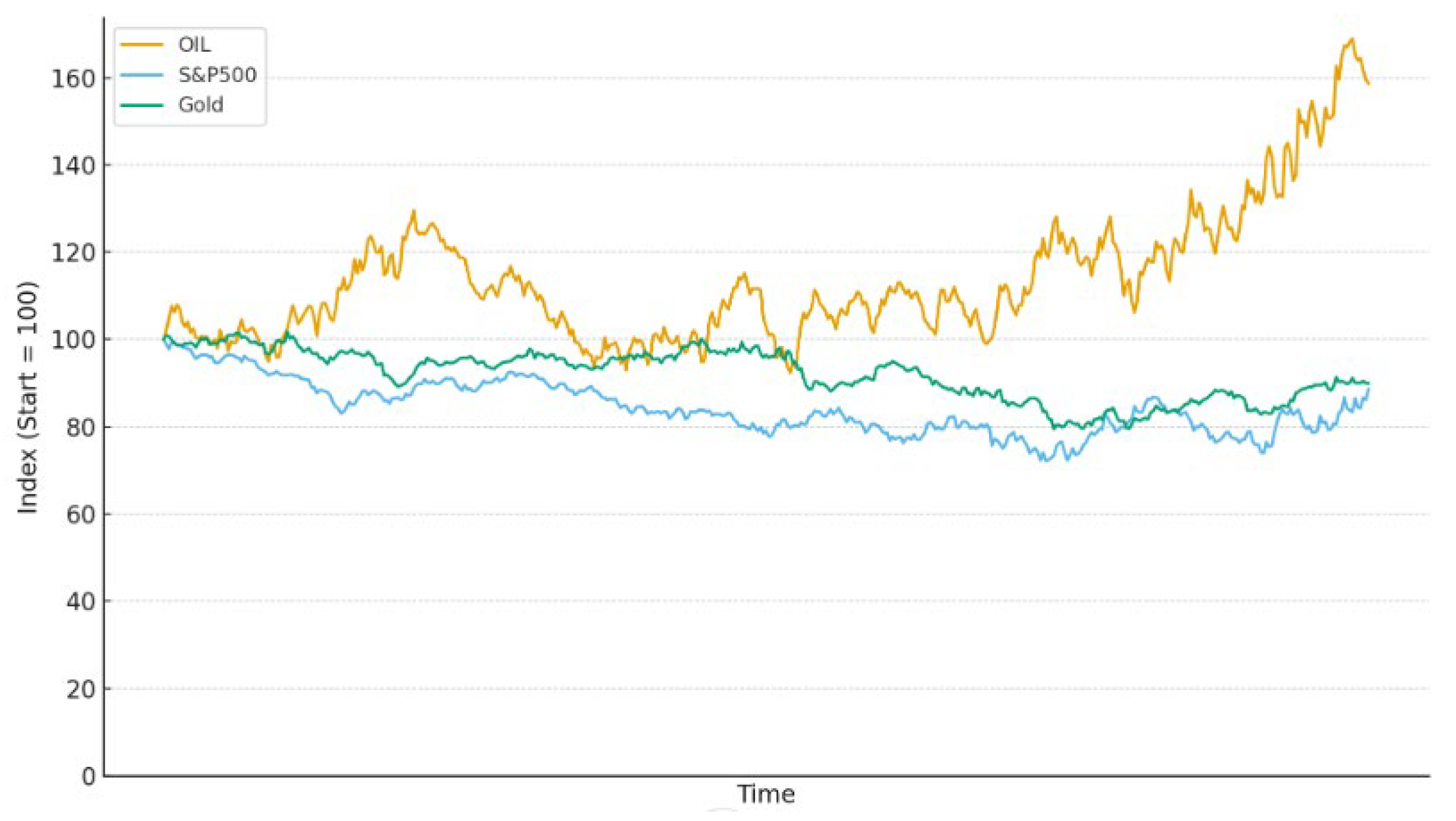
Figure 3 shows that during 2023–2024, oil prices rose while both Gold and the S&P500 declined.

We start our analysis with a stepwise multiple regression model that reduces the explanatory variables to the following (Model 1):

$$Oi{l}_t=0.002-0.112VI{X}_t+0.027OV{X}_t-0.008MOV{E}_t+0.005Gol{d}_t+0.009S\&P500+{\epsilon }_t$$

p-value    (0.042)    (0.001)    (0.003)    (0.003)    (0.214)    (0.416)

R² = 0.504

The regression reveals that oil price trends are positively influenced by its own volatility factor (OVX) and negatively by equity and bond volatility proxies. This result demonstrates how sensitive oil prices are to risk in their own environment and in other sectors of the economy. Residual analysis showed no autocorrelation (Durbin–Watson = 2.0) but heavy tails, suggesting volatility clustering. We applied Model 2 to capture short-term momentum in the oil price.

$$Oi{l}_t=0.871+0.513Oi{l}_{t-1}+{\epsilon }_t$$

p-value    (0.001)    (0.001)

R² = 0.263

The results confirm the presence of a positive autoregressive influence of yesterday’s oil price on the current oil price. To capture time-varying volatility, we used the ARCH(1) procedures (Model 3).

$${\sigma }_t^2=0.871+0.513{\epsilon }_{t-1}^2+{\mu }_t$$

p-value    (0.00)    (0.00)

R² = 0.375

The results of this model confirm that 51.3% of today’s volatility is explained by yesterday’s squared return shocks, indicating strong persistence in conditional variance. The level of 0.871 (α₀) represents the long-run average volatility level. The results of the PCA analysis are presented in

Table 1. PCA.

Variable	PC1	PC2	PC3
VIX	0.5731
OVX	0.3938
MOVE	0.3221
FRED	−0.1796	−0.3302	0.5953
S&P500	−0.5542	0.12128	−0.0926
3-Year Yields		0.4721	0.2809
Gold		0.0884
10-Year Yields		−0.3671	−0.2290

Notes: VIX = equity volatility index, OVX = oil price volatility index, MOVE = U.S government bonds volatility index, FRED = Federal Reserve Economic Data. 3-Year Yields = 3-year U.S government bonds yields, 10-Year Yields = 10-year U.S government bonds yields.

.

Principal Component 1 (PC 1) assigns large positive weights to volatility indices (VIX, OVX, and MOVE) and a strong negative weight to the S&P 500 return, so high PC 1 scores coincide with turbulent, risk-off episodes in which equity prices sag and option-implied volatility spikes. Because volatility variables move together, this single axis absorbs much of their shared variance and ends up explaining the largest slice (11%) of total variability. Principal Component 2 (PC 2) isolates a yield curve twist. It loads positively on the 3-year Treasury yield but negatively on the 10-year yield and the term-spread, meaning it rises when short-term yields rise relative to long-term yields, which might indicate a curve flip and a nearby recession. Principal Component 3 (PC 3) reflects a macro-liquidity commodity factor. It shows strong positive weights on the FRED liquidity proxy while still carrying a modest negative weight on the term spread. When PC 3 climbs, liquidity conditions appear loose, and commodity prices rise. Finally, we constructed seven statistical procedures to deepen our understanding of oil price behavior and identify nonlinear influences on its price. In addition, we constructed the meta-learner model (Figure 1) and reported all models’ predictive performances in

Table 2. Oil prediction models’ performances.

Model.	RMSE	MAE	Train R2	Tested R2
Meta-learner	2.04	1.65	0.852	0.532
Random Forest	2.17	1.72	0.814	0.482
Gradient Boosting	2.29	1.83	0.297	0.239
SVR	2.79	2.13	0.206	0.216
ARIMA	9.51	2.49	0.060	0.058
ARIMAX	9.80	2.76	0.062	0.058
ETS	9.94	2.46	0.054	0.053
LassoCV	10.37	2.48	0.205	0.186
Naïve Forecast	12.45	2.67	0.000	0.000
Random Walk	12.51	2.69	0.000	0.000

Notes: SVR = support vector regression; Naïve Forecast assumes tomorrow’s price equals today’s price. Random Walk assumes random fluctuations around the current value.

and Figure 4 using the RMSE (Root Mean Square Error) and MAE (Mean Absolute Error), which are two common metrics used to measure the accuracy of predictions.

Table 2 and Figure 2 demonstrate that the meta-learner, which is a combination of the three leading models, outperformed all the single models with an RMSE of 2.04, an MAE of 1.65, and a test R² of 0.532. These results are far stronger than standard baselines (Naïve Forecast and Random Walk), which achieve essentially no explanatory power (R² ≈ 0) and better predict oil price changes than any single tested model. While R² = 0.532 may appear modest, it is higher than other forecasting methodologies used in other studies using ARIMA-GARCH [9,11] or hybrid decomposition models [4,7], which typically achieve R² values in the range of 0.05–0.20, while machine learning approaches such as gradient boosting and neural networks [1,2] report modest improvements (R² up to 0.30).

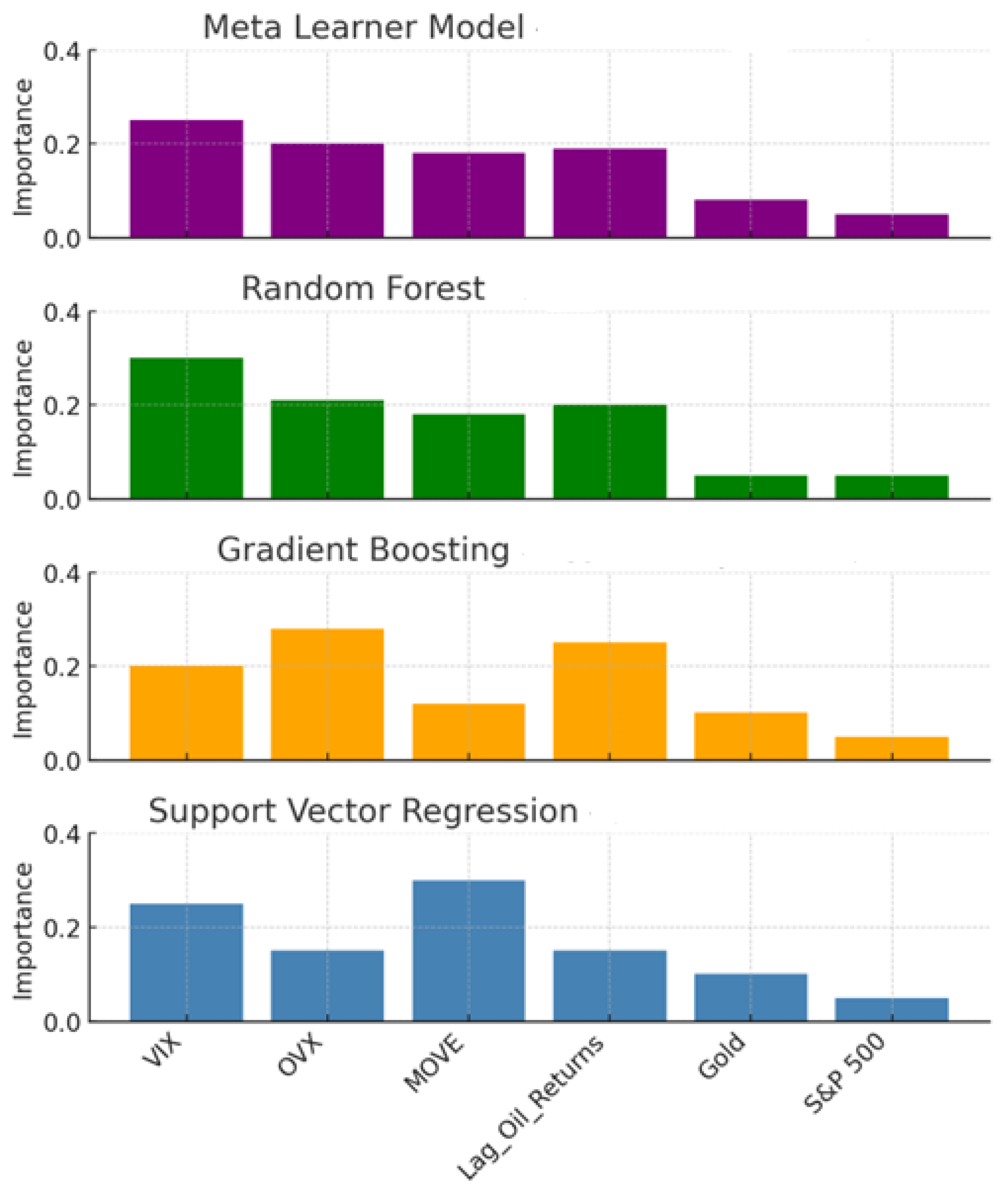
Out of the single models, the Random Forest was found to be the best model, exhibiting a test R² of 0.482, followed by gradient boosting and SVR (test R² of 0.239 and 0.216, respectively). Figure 5 shows the relative importance of the six most influential factors for each single model and for the meta-learner model, which consists of the three leading separate models.

In Figure 5, we learn that the six most important potential factors influencing oil prices are VIX, OVX, MOVE, lagged oil returns, Gold, and the S&P 500. Although the relative importance of each factor varies across models, the meta-learner model, which outperforms all others, suggests that volatility indices (VIX, OVX, and MOVE) provide timely information that may be valuable as early warning signals for risk managers and traders, although their predictive power remains moderate and should be interpreted with caution. 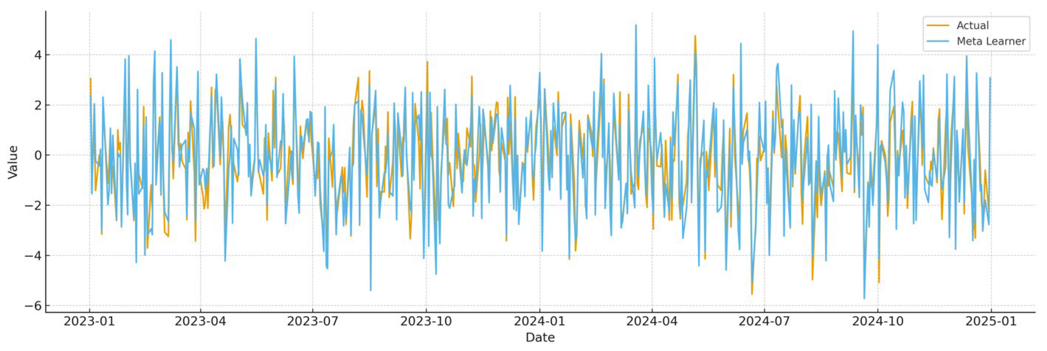Figure 6 and

Table 3. The meta-learner’s prediction power 2023–2024.

Actual Mean	Meta-learner Prediction Mean	Actual Std. Dev	Meta-learner Std. Dev.	MAE	MSE
−0.139	−0.111	1.775	1.987	0.684	0.712

Notes: MAE = average absolute error, MSE = average squared error.

demonstrate the predictive power of the meta-learner model over the period of 2023–2024.

The analysis of the 2023–2024 test period shows that the meta-learner produces forecasts that are well aligned with the actual behavior of oil returns. The average daily return of the actual series was −0.139, while the meta-learner predicted a nearly identical mean of 0.111, indicating that the model is not systematically biased. In terms of volatility, actual returns fluctuated with a standard deviation of 1.78, while the model predicted a slightly higher spread of 1.99, reflecting a modest tendency to overestimate market swings. Forecast accuracy measures confirm solid performance: the average absolute error was 0.68, and the average squared error was 0.71, suggesting that deviations from actual values were moderate and extreme misses were rare. These results demonstrate that our model not only tracks the central tendency of oil prices but also captures their variability with reasonable precision, providing forecasts that are both statistically robust and practically useful. Figure 7 shows the directional accuracy test results for the years 2020 to 2024.

The directional accuracy test over the 2020–2024 period demonstrates that the meta-learner consistently predicts the sign of daily oil price changes with substantial reliability. Accuracy ranged from 71.4% in 2020 to a peak of 79.7% in 2021, stabilizing around 72–75% in subsequent years. These results demonstrate that the model is effective at identifying upward versus downward movements, providing a practically valuable signal for timing and hedging strategies.

5. Summary and Conclusions

This study reassessed the short-term predictability of daily crude oil prices by combining traditional econometric techniques with a stacked ensemble of machine learning models. Using ten years of daily data covering 21 financial and commodity variables (2015–2024), we estimated seven forecasting frameworks. Among the individual models, Random Forest achieved the strongest out-of-sample fit. However, the stacked meta-learner combining Random Forest, gradient boosting, and support vector regression predictions through a second-stage gradient boosting model outperformed all individual approaches. While volatility indices such as VIX, OVX, and MOVE show moderate predictive power, they should be interpreted as potential early warning signals rather than definitive predictors that can be used by risk managers and traders for hedging and asset allocation. Feature-importance diagnostics converged on four dominant predictors: the volatility indices VIX, OVX, and MOVE, together with the one-day lag of oil returns, with Gold and the S&P 500 playing a secondary role. These results confirm our hypotheses that volatility spillovers and short-term momentum are central drivers of oil price dynamics, and that ensemble learning methods can meaningfully outperform both classical econometric models (e.g., ARIMA and ETS) and individual ML models.

Methodologically, this study contributes by demonstrating how dimensionality reduction via PCA, combined with a carefully structured stacked ensemble, enhances predictive performance in volatile and nonlinear commodity markets. The limitation of this research is that the model’s explanatory power, while strong relative to benchmarks, is moderate in absolute terms, reflecting the inherent unpredictability of oil markets. Future research could improve forecasts by incorporating macroeconomic indicators, news and sentiment data, and more advanced deep learning architectures such as LSTMs or transformers. Extending the framework to intraday data or cross-market comparisons represents another promising avenue.