Article

Exploratory Proof-of-Concept: Predicting the Outcome of Tennis Serves Using Motion Capture and Deep Learning

by
Gustav Durlind
1,
Uriel Martinez-Hernandez
1,2 and
Tareq Assaf
1,*
1
Department of Electronic and Electrical Engineering, University of Bath, Bath BA2 7AY, UK
2
Multimodal Interaction and Robot Active Perception (Inte-R-Action), University of Bath, Bath BA2 7AY, UK
*
Author to whom correspondence should be addressed.
Mach. Learn. Knowl. Extr. 2025, 7(4), 118; https://doi.org/10.3390/make7040118
Submission received: 22 July 2025 / Revised: 2 October 2025 / Accepted: 11 October 2025 / Published: 14 October 2025

Abstract

Tennis serves heavily impact match outcomes, yet analysis by coaches is limited by human vision. The design of an automated tennis serve analysis system could facilitate enhanced performance analysis. As serve location and serve success are directly correlated, predicting the outcome of a serve could provide vital information for performance analysis. This article proposes a tennis serve analysis system powered by Machine Learning, which classifies the outcome of serves as “in”, “out” or “net”, and predicts the coordinate outcome of successful serves. Additionally, this work details the collection of three-dimensional spatio-temporal data on tennis serves, using marker-based optoelectronic motion capture. The classification uses a Stacked Bidirectional Long Short-Term Memory architecture, whilst a 3D Convolutional Neural Network architecture is harnessed for serve coordinate prediction. The proposed method achieves 89% accuracy for tennis serve classification, outperforming the current state-of-the-art whilst performing finer-grain classification. The results achieve an accuracy of 63% in predicting the serve coordinates, with a mean absolute error of 0.59 and a root mean squared error of 0.68, exceeding the current state-of-the-art with a new method. The system contributes towards the long-term goal of designing a non-invasive tennis serve analysis system that functions in training and match conditions.

1. Introduction

Since its creation in the early 1800s [1], tennis has grown to become one of the largest sports in the world, with the International Tennis Federation reporting 87 million players globally [2]. Additionally, tennis has a rich history of technological development, including continued research into materials for rackets and ball aerodynamics [3,4]. However, with advances in camera technologies in the early 2000s and advances in AI and ML, research has shifted towards computer vision-based articles.
The serve is one of the most crucial elements of tennis and can heavily determine the outcome of a match. Therefore, for effective sports performance analysis in tennis, it is critical to have robust systems to analyse tennis serves. Whilst tennis coaches can leverage years of experience to highlight faults in a player’s technique, they are limited by biases and the human vision system. An automated tennis serve analysis system could provide objective information and data at precisions impossible to the human eye. Creating a system to analyse tennis serves has historically been seen as a sports video classification problem due to the large quantities of available video data for tennis. However, this requires computationally intense and complex pose estimation algorithms to extract three-dimensional data. Recent advances within marker-based and markerless motion capture systems suggest that three-dimensional datasets could be produced and harnessed to analyse tennis serves.
This work details the collection of three-dimensional marker-based motion capture data along with a proof-of-concept for the design of a novel two-part ML powered system, that can accurately classify serves into three categories: “in”, “out”, or “net” and then proceed to predict the serve coordinate location, using solely marker-based motion capture data and ML models.
The initial implementation of electronic technology within tennis started with the “Cyclops” machine for line calling in the 1980s [5], which was superseded by Hawk-Eye’s ground-breaking 2006 line calling system [6]. The Hawk-Eye system has continued to provide the current state-of-the-art ball trajectory tracking within tennis, as well as cricket, badminton, snooker and association football [6]. Following this, IBM created iterations of real-time dashboards in 2008 and 2012 that provided information on matches and players on a point-by-point basis [7]. As Hawk-Eye continue to pioneer technology for umpiring systems, and IBM focus on enhancing the fan experience, the future of innovation for tennis lies within its players. This includes wearable technology, smart rackets and smartphone applications that feed information to the player on their performance.
Bartlett introduced the concept of sports performance analysis in 2001 [8] by combining biomechanics and notational analysis. This involved the study of bodily movements as well as contextual information. The serve is a closed skill where the player has total control of the outcome through the kinetic chain produced within their body [9], therefore biomechanical analysis provides the most impactful information for performance analysis.
The methods of data collection for performance analysis in tennis have evolved significantly as technology has progressed. The four major forms of primary data collection are tracking technologies, video images, data mining, and observations of coaches [10]. This work uses motion capture tracking technology for data collection. Whilst markerless motion capture could provide an accessible and non-invasive tool for the analysis of tennis serves, improved results for these systems would require richer datasets to achieve computational parsimony [11]; therefore, the gold standard for motion capture is still marker-based optoelectronic motion capture. Markerless motion capture systems could also further benefit in the future from using pre-trained ML models that harness marker-based data. The ML models used within this work were chosen based on proven functionality within similar classification and prediction tasks.
The system was validated against the current state-of-the-art for tennis serve classification and prediction. The validation metrics include: accuracy, mean absolute error and root mean squared error. The rest of this paper is organised as follows: The related work is presented in Section 2. The materials and methods are detailed in Section 3. The results, discussion and conclusion are presented in Section 4, Section 5 and Section 6, respectively.

2. Related Works

2.1. Video Analysis with Computer Vision

The first category of tennis serve analysis systems encompasses processes that use computer vision techniques to extract biomechanical and notational data from videos. The principle of operation for these systems involves multiple cameras and advanced computational algorithms to triangulate points in 3D space. As Hawk-Eye and the Grand Slam Board have exclusive access to the spatio-temporal data collected within professional matches [12], researchers have been compelled to derive this data from publicly available video data or manually created datasets.
Despite being a heavily televised sport, there is a fractured data landscape [13], leading to the Match Charting Project (MCP) in 2015, a crowd-sourcing effort to collect detailed records of all professional tennis matches on a shot-by-shot basis. This has facilitated research for articles on players’ serial dependencies on serve directions [14] and the probability of winning service games for various serve directions [15]. More recently, the MCP was used by Zhu and Naikar in 2023 to predict tennis serve directions using ML [16]. Zhu and Naikar split the service box into three parts, commonly denoted in tennis as “wide”, “body”, and “T” (centre of the court). Through feature engineering and a series of ML models, they managed to predict serve directions at 49% accuracy for male players and 44% for female players.
Whilst publicly available videos have enabled notational analysis of serves and serve predictions, spatio-temporal data at skeletal precision has not been achieved. Therefore, in 2013 Gourgari et al. produced the THETIS database, a comprehensive set of 8374 videos depicting 24 experienced players and 31 amateurs performing 12 different tennis actions [17]. THETIS was used in 2020 by Xia and Lee to classify the serves into three categories: Flat, Kick and Slice [18]. Their model reached 54.9% accuracy using a combined InceptionV3 and Long Short-Term Memory (LSTM) model architecture. Following this, Sen et al. harnessed the Xception pre-trained model and a Convolutional Neural Network (CNN) and LSTM architecture to achieve 75% accuracy in classifying all twelve shots from the THETIS dataset [19]. Despite being the most complete and robust use of the THETIS dataset, the article noted that the model struggled disproportionally with classifying the different serves, achieving 62.6% accuracy in classifying the serves into Flat, Kick and Slice categories. Similar trends were seen in other publications classifying all 12 shots from the THETIS dataset [20,21,22,23]. Additional publications have analysed tennis serves by creating new datasets. Jabaren produced a dataset of videos from two camera angles, filming professional players and players with no experience completing the three serve types [24]. Using a Stacked Bidirectional LSTM architecture and the Resnet-50 pre-trained model, an accuracy of 85.7% was achieved in classifying between amateur and professional serves. Whilst this method produced the highest accuracy, it is discussed within the research that more data would be required to expand the system beyond its binary classification.

2.2. Motion Tracking Technology

The second category of tennis serve analysis systems involve using multi-camera setups to provide 3D trajectories for ball and player tracking. The principle of operation for these systems includes the use of multiple high-speed cameras which process video feeds in a synchronised manner to provide 3D triangulation for points of interest. Hawk-Eye operates at the current state-of-the-art for ball trajectory tracking within tennis and has allowed access to their data for various studies analysing tennis serves. Player tracking for the biomechanical analysis of tennis serves can be completed through marker-based or markerless motion capture systems.
Despite the private nature of Hawk-Eye’s spatio-temporal data, various publications have been granted access for research purposes. Notably, in 2015, Wei et al. used the 3D data from 7050 serves to create a system to predict serve direction [25]. Using contextual information as well as analysis of the ball trajectories, Wei et al. achieved an accuracy of 27.8% when classifying the direction of the serve into seven categories. Whiteside and Reid then used data from 25,680 serves to determine the features of an ideal serve [26]. They achieved an accuracy of 87% for classifying if a serve would be an ace or not. Moreover, they found that directionality and ball placement are more critical for serve success than speed. An additional study from Tea and Swartz utilised ball trajectory data from Infosys’s CourtVision [27]. Using Bayesian Multinomial Logistic Regression, a predictive model was built for serve direction; however, accuracies for individual players were not reported. The only accuracy reported included a 64% accuracy for predicting Roger Federer’s serve direction.
Motion capture technology has existed through various iterations for decades for entertainment, sport and medical purposes. Marker-based motion capture relies on high-contrast video imaging of reflective markers attached to the body. This technology has been used effectively for analysis within other sports, including judo [28] and golf [29]. Whilst there are many publications using marker-based motion caption for tennis serve analysis [30,31,32,33], and there are multiple articles using marker-based motion capture for tennis stroke classification [34,35,36], there are no publications for tennis serve classification using marker-based motion capture for data collection. Similarly, whilst markerless motion capture systems have been used for tennis serve analysis [37,38,39], the systems cannot achieve the measurement accuracies of marker-based motion capture systems in an accessible manner. This was reinforced in a recent 2023 study where Emmerson et al. designed a novel state-of-the-art markerless motion capture system and compared it with the current gold standard for marker-based motion capture for analysing tennis serves [40]. The research achieved similar performance for the markerless system as seen with the gold standard provided through marker-based motion capture and further confirmed the potential for markerless systems as a non-invasive monitoring tool. However, it is discussed that further work is required within the field to validate the system for additional tennis-specific movements. Moreover, the method requires expensive equipment and highly qualified staff for data collection and analysis, reducing accessibility to the technology. Therefore, whilst markerless motion capture for tennis serve analysis shows promise from laboratory results, marker-based motion capture is still currently the gold standard.
Whilst it is proven serve location affects the success of the serve [26,41], only recently has there been a proof-of-concept for a system that can predict the serve location from biomechanical data. This research was published by Ye et al. in 2024 [42] and detailed a system that uses data from inertial sensors on a participant’s body to predict the serve location and serve speed, as well as identify faulty actions. Despite using an alternative form of data collection, this literature’s significance lies in providing the current state-of-the-art for serve prediction as a regression task instead of a classification task. Using an attention-based CNN model, the system’s predictions achieved 0.72 mean absolute error (MAE) and 0.98 root mean squared error (RMSE).

3. Materials and Methods

3.1. Experimental Setup

Two right-handed male participants (181 cm and 178 cm) were recruited and provided written informed consent. The participants performed 175 flat serves each from the deuce side of an indoor tennis court, positioned 50 cm to the right of the centre mark. The participants were fitted with a full-body marker set each, as designed by Emmerson et al. in accordance with the gold standard of measurements for three-dimensional kinematics [40]. This consisted of 31 individual markers and a series of clusters made up of 44 additional markers, shown in Figure 1C.
The clusters allowed for bilateral tracking of thighs, shanks, feet, upper arms, forearms and hands, as well as tracking the participant’s pelvis, thorax and head. Additionally, the participant’s rackets were fitted with three markers, one at either side of the outermost point on the racket rim and one at the base of the racket head. Motion data was captured with an eight-camera marker-based motion capture system consisting of Qualisys Miqus M5 motion capture cameras (Qualisys, Gothenburg, Sweden) operating at 180 frames per second with 4 MP (2048 × 2048) resolution, the highest sampling frequency available at this resolution. These cameras are shown in Figure 1A, with stills shown in Figure 2. The cameras were positioned 3.5 m from the participants to allow for a 48 m3 capture volume (4 m × 4 m × 3 m), in controlled lighting. As shown in Figure 1B, the opposing deuce service box was fitted with 62 marking lines positioned 50 cm apart, starting from the intersection of the service line and the centre service line. To record the position of the serve outcome, a high-speed Miqus video camera was fitted to a 3 m tripod and positioned 8.5 m from the service box at a 45-degree angle. The motion capture system and video camera were spatially aligned and time-synchronised with a frame-locked sampling frequency of 180 Hz for simultaneous collection of data. Figure 1 shows an illustration of the entire on-court experimental setup used for the collection of the data. The hardware requirements to train models include a Linux Ubuntu 20.04.1 OS, Python 3.8.10, 11th Gen Intel© Core™ i9-11900 @ 2.50 GHz processor and NVIDIA GeForce RTX 3080 graphics with 62 GB 1600 MHz DDR3 of memory (University of Bath AI Laboratory, Bath, United Kingdom).

3.2. Data Pre-Processing

3.2.1. Motion Data

All marker trajectories were labelled and gap-filled using Qualisys Track Manager (Qualisys, Gothenburg, Sweden). An Automatic Identification of Markers (AIM) model was developed from a static recording of the participants, and continually improved for each serve completed. In the case of occluded markers, the gaps in the trajectories were filled through a polynomial or virtual technique. The polynomial method involves using an algorithm and the X, Y and Z coordinates on either side of the gap to interpolate the missing trajectories. This method was used for any gaps that were smaller than 10 frames, as the algorithm becomes increasingly erroneous for larger gaps. The virtual method for gap filling is based on the movement of surrounding markers. Up to three contextual markers can be selected and an offset can be applied to produce an accurate trajectory for the gap. Due to the high number of markers and clusters used, sufficient contextual information was available to fill all gaps for all 75 markers. A moving average filter was then used to smooth any spikes in the data caused by discontinuities between consecutive frames. Each serve was then trimmed to 301 frames from the original 1080 frames to ensure the ML model was only trained on relevant information. The serves were then exported from QTM as MATLAB files (.mat) where each file was a 3D array of information representing frames, markers and the X, Y and Z coordinates (301 × 75 × 3). MATLAB (R2024a) scripts were then written to automate reformatting the data into 3D and 5D tensors for the various ML models.

3.2.2. Serve Outcome Data

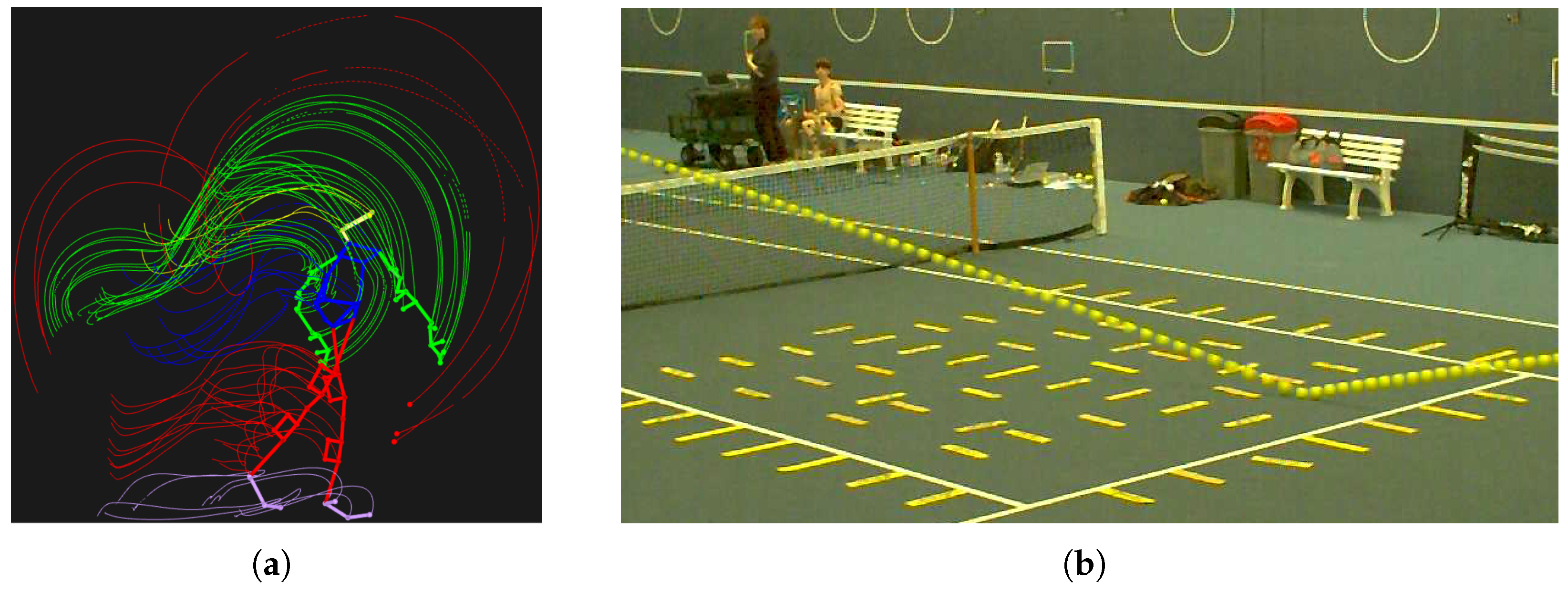
Along with the motion capture data for each serve, an accompanying 6 s video showed the position of where the ball landed within the service box. As these videos were recorded at 180 fps and the marking lines were placed 50 cm apart, the coordinates of the serve could be calculated to the precision of 0.1 m from the frame in which the ball is bouncing. Each of the 350 videos was manually processed with the coordinates stored in Excel. Figure 3 shows the trajectory of the serve seen within each video, as well as the distinct frame in which the ball bounced. The videos also concluded if the serve hit the net or went out, with these serves being given a binary label of “net” and “out”, respectively, for the classification model. Any serve that hit the net and bounced in/out (let), was categorised as an anomaly and excluded from the dataset as the trajectory of this serve would not accurately be represented by its outcome. The data was then imported into MATLAB from Excel and MATLAB scripts were written to reformat all the labels for the classification and regression task. The labels for the classification task required a one-dimensional array of integers between 1 and 3, representing “in”, “out” and “net”, respectively. The regression task required a two-dimensional array of coordinates with the two columns representing the X and Y values, and each row representing a serve. Table 1 shows the distribution of serve outcomes between the four categories.
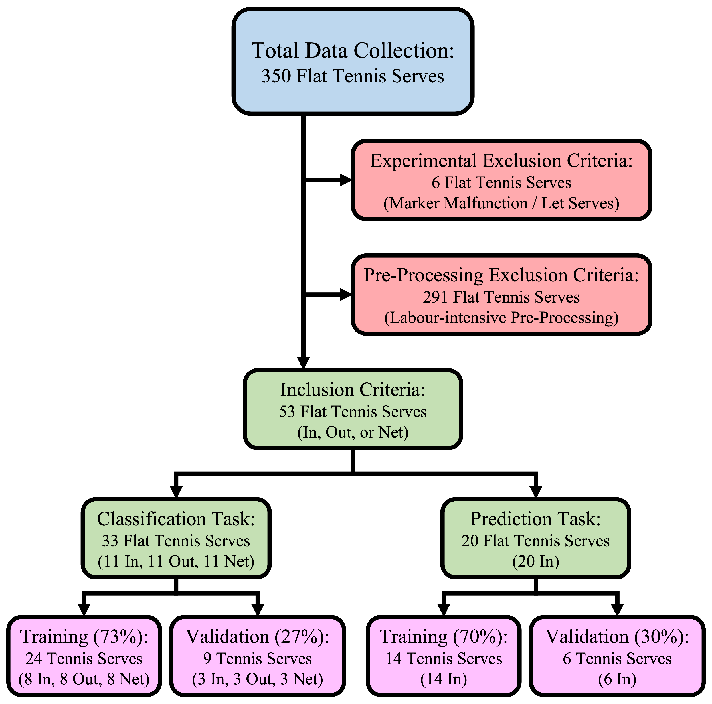
A complete data inclusion/exclusion flow chart is shown in Figure 4. In total, data from 350 flat tennis serves was collected, with 6 serves immediately excluded due to faulty markers and “let serves”. Following this, due to the labour-intensive nature of the data pre-processing, only 53 serves were fully processed for the models. For the classification task, a subset of 33 serves was randomly selected maintaining even distributions of serve outcomes from both participants (17 serves from Participant 1 and 16 serves from Participant 2). For the prediction task, 20 serves were selected (10 from each participant), prioritising coverage of the feature space through a wide spread of serve coordinates. This allows the regression to generalize across different trajectories.

3.3. Machine Learning Models

3.3.1. Stacked Bidirectional LSTM

A Stacked Bidirectional LSTM model was used for the classification of the tennis serves. This model was chosen due to its proven capabilities within the handling of sequential data for classification [18,19,21,22,24,43]. Out of the 33 serves chosen for the model, 24 serves were used for training (8 in, 8 out and 8 net) and 9 were used for validation (3 in, 3 out and 3 net). This ratio fits within the industry standard of having 20–30% of data used for testing and the remaining 70–80% of data used for training [44].
The 2D arrays from MATLAB were concatenated into two 3D tensors, one for training the model and one for validating the model. These 3D tensors were structured so that the first element represented the number of serves within the 3D tensor (24 or 9), the second element determined the number of frames per serve (301), and the final element represented the number of features per serve (225). In order to fit the data into the 3D tensor framework, the data for each frame of each serve was flattened into a 1 × 225 array, where each of the 75 markers had an X, Y and Z coordinate, resulting in 225 features. These 1 × 225 arrays were concatenated into a 301 × 225 array which represented each serve. Finally, these 301 × 225 2D arrays were stacked into a 3D tensor for all the serves. Creating a 24 × 301 × 225 3D tensor for training the model, and a 9 × 301 × 225 3D tensor for validating the model.
The LSTM network is an advanced Recurrent Neural Network (RNN) capable of capturing historical information within time series data [45]. Whilst RNNs can only store short-term information, LSTMs function through sets of gates (forget gate, input gate and output gate) that facilitate long-term and short-term memory along time steps [46]. This is due to its ability to recall long-term time-series data with an automatic control for retaining or discarding features in a cell state, whilst preventing vanishing gradient problems [47]. Therefore, LSTM networks are effective for pre-processing, classification, and prediction tasks based on time-series data. Figure 5 shows the LSTM architecture, with weights “W” and biases “B”.
Bidirectional processing allows for sequences in both directions within the network to be processed simultaneously, each with two separate LSTM hidden layers [48]. Therefore, Bidirectional LSTMs extract more features from the original input data and have been proven to outperform Unidirectional LSTM models in many fields.
Existing publications have shown a correlation between architectures with several hidden layers and increased performance for the model [49,50]. This is achieved through a higher level of representations of sequence data, leading to the model working more effectively.
Utilising both bidirectional processing and a stacked architecture with the LSTM will allow for the complex spatio-temporal information of the serves to be optimally analysed. This will include capturing the spatial correlation between markers, as well as the temporal dependencies between frames during the feature learning process [48].
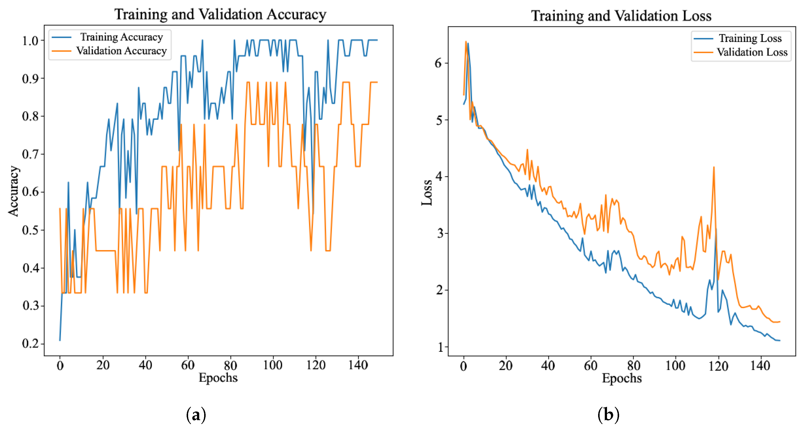
During the development of the Stacked Bidirectional LSTM, a series of optimisations were completed to increase accuracy and reduce loss. Initially, a grid search was completed for hyper parameter tuning of the additional stacked layers (2, 3, 4, 5 and 6) and hidden units (32, 64, 128 and 256). From this, four additional stacked layers and 256 hidden units performed best over 60 epochs. However, the system showed signs of overfitting so further optimisations were implemented, these include a grid search for Dropout Layers (0.1, 0.2, 0.3, 0.4 and 0.5) and L2 Regularization ( λ ) (0.1, 0.2, 0.3, 0.4, 0.5, 0.6 and 0.7). A Dropout Rate of 0.1 consistently produced the highest accuracies with lowest loss. Introducing the large weight decay of λ = 0.7 within the final layer reduced overfitting, at the cost of slower convergence. Therefore, the number of epochs was increased incrementally to 100, 150 and 200. Ultimately, 150 epochs allowed for the strong L2 regularization to reduce overfitting whilst allowing the model to capture the spatio-temporal dependencies, as displayed in Figure 6.
The Stacked Bidirectional LSTM model was created using TensorFlow’s Sequential Model and the Keras layers: LSTM, Bidirectional, Dropout and Dense, along with Keras’ Adamax Optimiser. Random seeds and model weights were achieved through TensorFlow’s default randomized settings. The final design includes:
  • Five Bidirectional Layers: Using 256 hidden units within each layer;
  • Five Dropout Layers: Set with a Dropout of 0.1;
  • Two Dense Layers: With 128 and 3 units, respectively. L2 Regularization ( λ = 0.7) was applied only to the final Dense Layer, which also used “softmax” activation;
  • Total parameters: 7,352,835.
Whilst the parameter count is high relative to the dataset size, which increases the risk of subject-specific overfitting, the application of strong regularization techniques, combined with an increased number of training epochs, allowed the model to converge while reducing the likelihood of memorising subject-specific idiosyncrasies.

3.3.2. The 3D Convolutional Neural Network

A 3D Convolutional Neural Network was used for the prediction of the tennis serves. This was implemented due to its proven capabilities within regression tasks for 4D data [51]. Out of the 20 serves chosen for the model, 14 were used for training and 6 were used for validation. As with the classification task, this split lies within the 70/30 and 80/20 ratios seen as the industry standard [44].
The 3D MATLAB arrays representing the serves were stacked into two 5D tensors, one for training and one for validation. These 5D tensors were structured so that the first element represented the number of serves (14 for training and 6 for validation), the second element includes the number of frames per serve (301), the third element gives the height of each frame (the 75 separate markers), the fourth element is the width of each frame (the X, Y and Z coordinates for each marker), and the final element represents the channels (1). This fifth element was added as the Conv3D and Maxpooling3D layers require a 5D tensor input, however, as this is set to ‘1’, the 5D tensor acts as a 4D array. Therefore, the 5D tensors were 14 × 301 × 75 × 3 × 1 for the training data and 6 × 301 × 75 × 3 × 1 for the validation data.
CNNs are artificial neural networks that have become dominant within the field of computer vision by adaptively learning spatial hierarchies of features between connected layers [52]. CNN architecture is based on three principles: local receptive fields completing feature extraction in local neighbourhoods, shared weights extracting features in a consistent manner, and subsampling reducing the size of the feature maps [53].
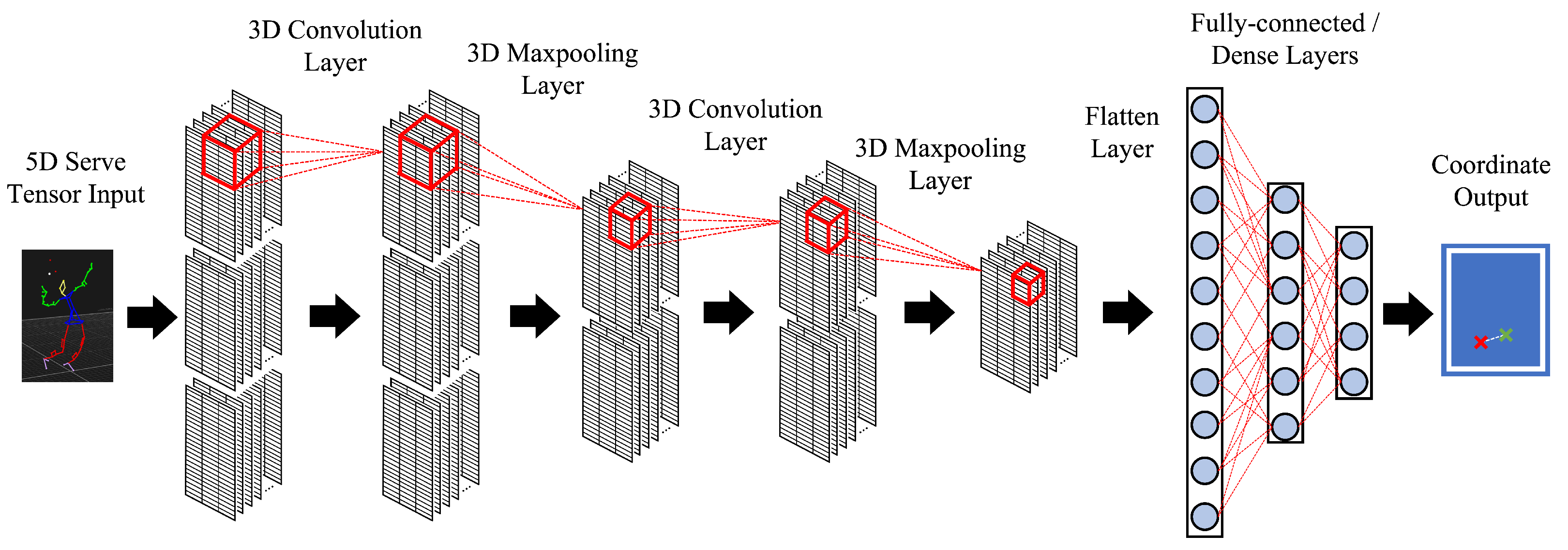
Leveraging these principles, Convolutional Layers perform dot product calculations between the kernel and the selected portion of the receptive field. Pooling layers subsequently reduce the size of the data, with the most common pooling operation being Maxpooling, which outputs the maximum output from the kernel. The data is then flattened and fully-connected layers (Dense Layers) map each neuron output from one layer to the input of the next. This reduces the size of the data towards the output required from the ML model. Whilst CNNs usually work with 2D data, they can be adapted to work with 3D data to form 3D CNNs. These function in an identical fashion, but use a 3D kernel to perform 3D Convolutions and 3D Maxpooling. Figure 7 depicts the operation of a 3D CNN for the purposes of predicting the outcome of a serve.
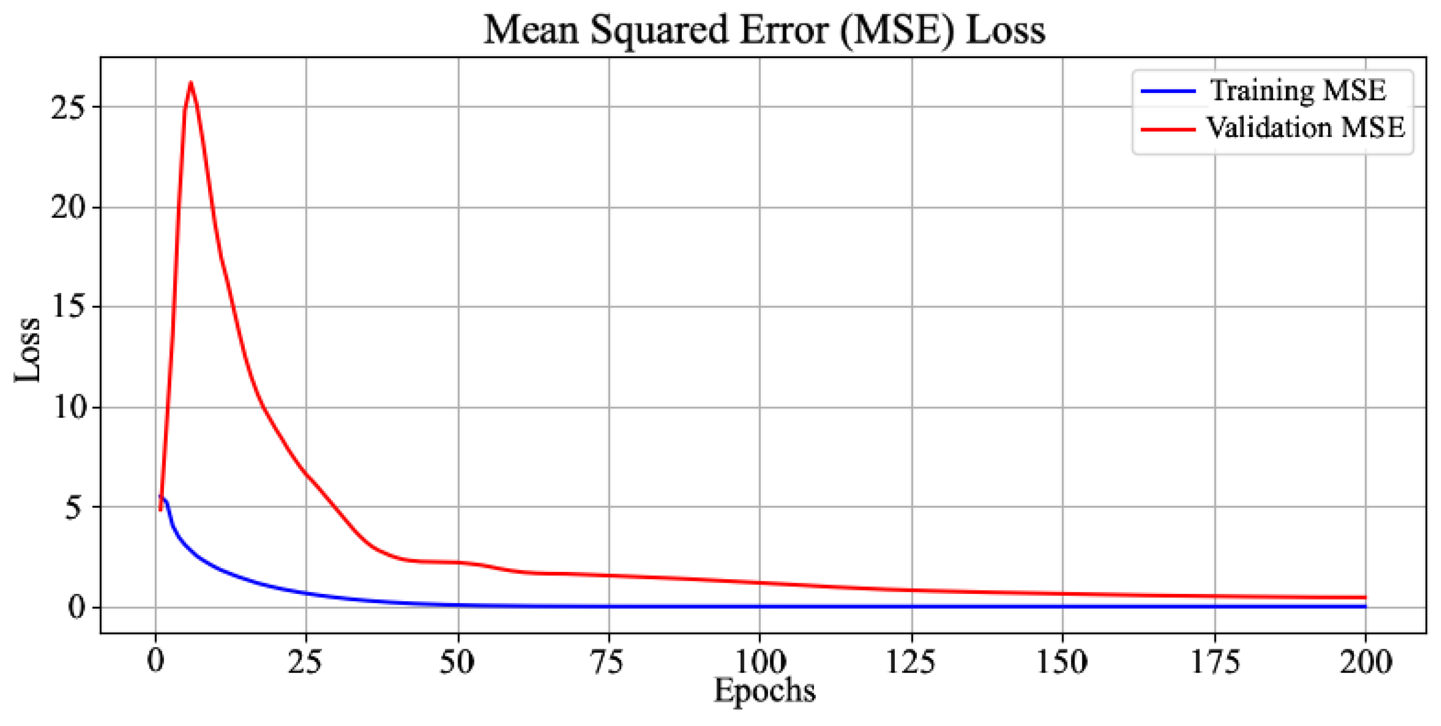
Throughout the development of the 3D CNN model, as with the Stacked Bidirectional LSTM model, a series of optimisations were completed. Due to the size and complexity of the input data, an architecture with an equal number of 3D Convolutional and 3D Maxpooling Layers was chosen to continually both learn features and reduce dimensionality. Initially, the grid search for hyper parameter tuning focused on ranges of Convolutional/Maxpooling Layers (1, 2, 3 and 4) with a variety of Dense Layers (1, 2, 3 and 4). As prediction accuracy is defined through disparity of coordinate distances, these optimisations were evaluated through Mean Squared Error (MSE) loss. This grid search showed the optimal combination includes three Convolutional/Maxpooling Layers and one Dense Layer, over 100 epochs. Following this, to further investigate convergence, the model was run over 100, 200 and 300 epochs. With clear overfitting being seen towards 300 epochs, 200 epochs provided the lowest loss for the 3D CNN model, as shown in Figure 8.
The 3D CNN model was designed using TensorFlow’s Sequential Model and the Keras layers: Conv3D, MaxPooling3D, Activation, Flatten and Dense, along with Keras’ Adam optimiser. Random seeds and model weights were achieved through TensorFlow’s default randomized settings. The model requires one input argument representing the input shape of each serve. Therefore, the input shape is set to (None, 301, 75, 3, 1) to account for the varied number of samples, as well as all three spatial dimensions and the channel. The final design includes:
  • Three 3D Convolutional Layers: Using 32, 64, and 128 filters, respectively;
  • Three 3D Maxpooling Layers: Maxpooling sizes of (2, 2, 2) and padding set as “same”;
  • Three Activation Layers: Each activation layer set as “relu”;
  • One Dense Layer: With 2 units and “linear” activation;
  • One Flatten Layer: Placed between the Convolutional and Dense layers;
  • Total parameters: 180,290.

4. Results

4.1. Tennis Serve Classification

The Stacked Bidirectional LSTM designed with four additional LSTM layers, 256 hidden units, a 0.1 Dropout Rate and L2 Regularization (weight decay factor of 0.7) run over 150 epochs, consistently achieved validation accuracies up to 89% across multiple runs, with a validation Categorical Cross-Entropy loss of 1.43. The accuracy represents the number of true positives out of the number of total predictions while Categorical Cross-Entropy is the industry standard for loss within classification tasks as it calculates the dissimilarity between predicted and true labels. Figure 9a depicts the Normalised Confusion matrix for the classification.

4.2. Tennis Serve Prediction

The 3D CNN designed with three 3D Convolutional and Maxpooling layers, and one Dense Layer run over 200 epochs, achieved predictions that were within a 1 m radius of the actual coordinate at an average of 63% accuracy for the entire system over twenty runs. Furthermore, 98% of predictions were within a 2 m radius of the actual coordinate. Additionally, the average MAE was 0.59 and the average RMSE was 0.68. The accuracy of the coordinate predictions was measured in standard units (metres) to enable future work to compare in a more consistent manner than the arbitrary units designed by Ye et al. [42]. However, as with Ye et al.’s article, MAE and RMSE were used to measure error within the system due to their interpretability and sensitivity to outliers. Figure 9b plots the actual and predicted coordinates for all six validation serves over twenty runs.

5. Discussion

This work aims to propose a system for performance analysis of tennis serves by leveraging Machine Learning and marker-based motion capture to predict the outcome of the serve. Additionally, this work aims to act as a proof-of-concept for the compatibility of marker-based motion capture data on tennis serves for classification and regression tasks.
Whilst various publications exist within the field of tennis serve classification, the reported accuracies are not directly comparable with our system’s performance. This is due to the literature utilising video datasets and classifying serve actions (Flat, Slice and Kick) instead of classifying serve outcomes. However, with our system’s classification achieving 89% accuracy, whilst performing finer-grained classification within a single serve action, the performance provides a promising proof-of-concept for serve outcome classification. Existing publications propose that the future of tennis serve action classification lies within harnessing the vast amounts of video data that exists online, with assumptions that computer vision algorithms will continue to improve. However, our system proves that the future of tennis serve outcome classification could lie within motion capture and spatio-temporal data.
Ye et al. produced the highest accuracy within the field of prediction of tennis serves, achieving 92% of the predictions landing within three ’units’ of the actual coordinate, equating to a landing area of 2.40 m × 1.53 m. Additionally, their system achieved 75% accuracy for predictions within two ’units’ of the actual coordinate, equating to a landing area of 1.60 m × 1.02 m [42]. Our system achieved 63% accuracy for predictions within a 1 m radius of the actual coordinate, and 98% of predictions within a 2 m radius. As the definition of accuracy within this report involves a smaller radius, the lower accuracy relative to Ye et al.’s 75% could still be seen as performing in line with the current state-of-the-art. This point is further proven by the results in this report being disproportionately skewed by instability within the system, with 79% of the top twelve predictions out of the twenty runs being within a 1 m radius. Therefore, with access to more training and validation data, it could be assumed that system stability and accuracy would increase. This is seen from Ye et al.’s system, which was trained on 312 sets of data, in contrast to the 38 sets of data used in this report. This point is further proven as Ye et al. achieved a MAE of 0.72 and an RMSE of 0.98, whereas the system designed in this report accomplished a MAE of 0.59 and RMSE of 0.68.Therefore, the system designed in this report achieved lower average errors than, and accuracies in line with, the current state-of-the-art for tennis serve prediction from biomechanical data, using a novel method. The implications of these results for the field of tennis serve predictions include providing a novel method for the prediction of tennis serve outcomes.
The results further solidify that collecting biomechanical data is crucial for the design of a tennis serve analysis system, with all publications using notational data achieving lower accuracies with less precision. The underlying long-term goal for many of the publications within this field involves creating a non-invasive tool to analyse tennis serves at a precision that is unattainable for tennis coaches as they are limited by the human vision system and biases. This non-invasive tool could then be developed into an end-to-end system where users receive feedback on their technique during training, or being implemented in match settings. Whilst Ye et al. argue that inertial sensors have the most potential for cost-effective and accessible motion capture [42], our research proves marker-based motion capture continues to be the gold standard of movement recognition, and has the potential to facilitate applications with higher accuracy and better precision. Additionally, with the constant development of markerless motion capture systems, inertial sensors will continue to be the most cost-effective solution but have no potential to become a non-invasive tool. In contrast, the methodology from this report has the potential to be repeated with a markerless motion capture system when the gold standard of movement recognition becomes markerless. Moreover, the use of full marker trajectories, as opposed to predefined biomechanical features, results in our system being well positioned for future transfer learning to markerless motion capture, where similar spatio-temporal dependencies can be leveraged.
Alternatively, a complementary approach to our trajectory-based study could involve creating feature vectors from the serves, and developing models to map these feature vectors onto ball coordinates. Such an approach would facilitate feature ranking, providing interpretable insights into the most influential aspects of tennis serves. It could also incorporate biomechanical quantities, such as instantaneous velocity and acceleration, which are not directly represented in marker trajectories. Together, these allow for inherent probing of serve mechanics, in contrast to retrospectively probing the “black-box” architecture implemented in the present study.
Although the study demonstrates effectiveness in classifying and predicting tennis serves, various limitations should be considered. First, due to the dataset only being collected from two right-handed male participants serving on an indoor hard court, this limits demographic and environmental diversity. Therefore, the system would not be generalized to female players, left-handed players, or athletes with various ages and skill-levels. Additionally, the system performance could suffer when implemented on an outdoor court where wind and light become more difficult control variables to manage. Second, due to the time-intensive data pre-processing, only 53 serves were used for training and validation from the original 350 collected. This restricts overall system stability and robustness, with an increased risk of overfitting. Third, the system is yet to be validated on publicly available datasets or against classical models and sequence baselines, meaning external generalizability remains untested. Finally, despite marker-based motion capture being the gold standard for biomechanical data collection, this equipment is not widely accessible outside of laboratory and research settings for future studies. These limitations indicate that the current study should be viewed as a “proof-of-concept” rather than a definitive benchmark. Future works should focus on collecting a more diverse dataset, validating the models on existing datasets, benchmarking against classical models and introducing transfer learning to enhance data collected from markerless systems.

6. Conclusions

In this work, a system is proposed for tennis serve performance analysis through the prediction of the outcome of the serve. This is achieved by leveraging marker-based motion capture and Machine Learning. The classification task used 3D tensors and a Stacked Bidirectional LSTM to achieve 89% accuracy, whilst the prediction task used 5D tensors and a 3D CNN to achieve 63% accuracy with a MAE of 0.59 and an RMSE of 0.68. These results show promise within the field of tennis serve analysis systems, representing a proof-of-concept for the use of biomechanical data for finer-grain tennis serve classification, and for the compatibility of marker-based motion data with Machine Learning algorithms for precise coordinate predictions. Additionally, the results achieved accuracies exceeding the current state-of-the-art for both classification and predictions of tennis serves. Therefore, the findings from this work suggest the system designed can effectively be used as a tennis serve analysis system.
The findings from this report will also continue to be relevant as markerless motion capture systems are further developed, with the potential to be integrated into a completely non-invasive tool for analysis of tennis serves through transfer learning. However, improvements can be made in future works, most notably, the use of more serves and participants to increase system stability and generalization to unseen data. This includes a more diverse set of data collection, expanding on demographic and environmental diversity. Furthermore, feature vectors could be leveraged or the Machine Learning models could be probed to determine the most influential elements of a tennis serve, feeding back information to a player on specific points of interest for the player to focus on.

Author Contributions

Conceptualization, G.D. and T.A.; methodology, G.D., U.M.-H. and T.A.; software, G.D.; validation, G.D., U.M.-H. and T.A.; formal analysis, G.D., U.M.-H. and T.A.; investigation, G.D.; resources, U.M.-H. and T.A.; data curation, G.D., U.M.-H. and T.A.; writing—original draft preparation, G.D.; writing—review and editing, G.D., U.M.-H. and T.A.; visualization, G.D., U.M.-H. and T.A.; supervision, U.M.-H. and T.A.; project administration, T.A. All authors have read and agreed to the published version of the manuscript.

Funding

This research was funded by The University of Bath. IOAP Participant: University of Bath.

Informed Consent Statement

Informed consent was obtained from all subjects involved in the study.

Data Availability Statement

Data created during this research work is openly available from the University of Bath Research Data Archive at https://doi.org/10.15125/BATH-01454.

Acknowledgments

G.D. thanks Andreas Wallbaum and Julie Emmerson from the Applied Biomechanics Suite for their continued support, expertise and facilities. Additionally, G.D. thanks Fraser Barclay, David Kral, Shyam Prasad Shah, Rinki Goyal and Charles Nichols for their contributions to the completion of this research.

Conflicts of Interest

The authors declare no conflicts of interest.

References

  1. Crego, R. Sports and Games of the 18th and 19th Centuries; Bloomsbury Academic: New York, NY, USA, 2003. [Google Scholar]
  2. ITF. ITF Global Tennis Report; International Tennis Federation: London, UK, 2021. [Google Scholar]
  3. Lammer, H.; Kotze, J. Materials and tennis rackets. Mater. Sports Equip. 2003, 1, 222–248. [Google Scholar]
  4. Mehta, R.; Alam, F.; Subic, A. Review of tennis ball aerodynamics. Sports Technol. 2008, 1, 7–16. [Google Scholar] [CrossRef]
  5. Bal, B.; Dureja, G. Hawk Eye: A logical innovative technology use in sports for effective decision making. Sport Sci. Rev. 2012, 21, 107–119. [Google Scholar] [CrossRef]
  6. Chauhan, Y.S.; Pal, U.S. Innovative evolution of technology used among racket sports: An overview. J. Sports Sci. Nutr. 2022, 3, 175–179. [Google Scholar] [CrossRef]
  7. Larson, A.; Smith, A. Sensors and data retention in Grand Slam tennis. IEEE Sens. Appl. Symp. 2018, 1, 1–6. [Google Scholar] [CrossRef]
  8. Bartlett, R. Performance analysis: Can bringing together biomechanics and notational analysis benefit coaches? Int. J. Perform. Anal. Sport 2001, 1, 122–126. [Google Scholar] [CrossRef]
  9. Elliott, B.; Marsh, T.; Blanksby, B. A three-dimensional cinematographic analysis of the tennis serve. Int. J. Sport Biomech. 1986, 2, 260–271. [Google Scholar] [CrossRef]
  10. Takahashi, H.; Okamura, S.; Murakami, S. Performance analysis in tennis since 2000: A systematic review focused on the methods of data collection. Int. J. Racket Sport. Sci. 2022, 4, 40–55. [Google Scholar] [CrossRef]
  11. Desmarais, Y.; Mottet, D.; Slangen, P.; Montesinos, P. A review of 3D human pose estimation algorithms for markerless motion capture. Comput. Vis. Image Underst. 2021, 212, 103275. [Google Scholar] [CrossRef]
  12. Sorrentini, A.; Pianese, T. The relationships among stakeholders in the organization of men’s professional tennis events. Glob. Bus. Manag. Res. 2011, 3, 141–156. [Google Scholar]
  13. Kovalchik, S. Why Tennis Is Still Not Ready to Play Moneyball. Harv. Data Sci. Rev. 2021, 3. [Google Scholar] [CrossRef]
  14. Spiliopoulos, L. Randomization and serial dependence in professional tennis matches: Do strategic considerations, player rankings and match characteristics matter? Judgm. Decis. Mak. 2018, 13, 413–427. [Google Scholar] [CrossRef]
  15. Anderson, A.; Rosen, J.; Rust, J.; Wong, K.-P. Disequilibrium play in tennis. J. Polit. Econ. 2025, 133, 190–251. [Google Scholar] [CrossRef]
  16. Zhu, Y.; Naikar, R. Predicting tennis serve directions with machine learning. In Machine Learning and Data Mining for Sports Analytics; Brefeld, U., Davis, J., Van Haaren, J., Zimmermann, A., Eds.; Springer Nature: Cham, Switzerland, 2023. [Google Scholar]
  17. Gourgari, S.; Goudelis, G.; Karpouzis, K.; Kollias, S. THETIS: Three dimensional tennis shots, a human action dataset. In Proceedings of the 2013 IEEE Conference on Computer Vision and Pattern Recognition Workshops, Portland, OR, USA, 23–28 June 2013; pp. 676–681. [Google Scholar] [CrossRef]
  18. Ni, J.; Wang, J. Tennis serve recognition based on bidirectional long- and short-term memory neural networks. Mol. Cell. Biomech. 2025, 22, 1546. [Google Scholar] [CrossRef]
  19. Sen, A.; Hossain, S.M.M.; Uddin, R.M.A.; Deb, K.; Jo, K.-H. Sequence recognition of indoor tennis actions using transfer learning and long short-term memory. In Frontiers of Computer Vision; Sumi, K., Na, I.S., Kaneko, N., Eds.; Springer International Publishing: Cham, Switzerland, 2022; pp. 312–324. [Google Scholar]
  20. Vainstein, J.; Manera, J.F.; Negri, P.; Delrieux, C.; Maguitman, A. Modeling video activity with dynamic phrases and its application to action recognition in tennis videos. In Proceedings of the Progress in Pattern Recognition, Image Analysis, Computer Vision, and Applications, Puerto Vallarta, Mexico, 2–5 November 2014; Bayro-Corrochano, E., Hancock, E., Eds.; Springer International Publishing: Cham, Switzerland, 2014; pp. 909–916. [Google Scholar]
  21. Mora, S.V.; Knottenbelt, W.J. Deep learning for domain-specific action recognition in tennis. In Proceedings of the IEEE Conference on Computer Vision and Pattern Recognition (CVPR) Workshops, Honolulu, HI, USA, 21–26 July 2017; pp. 170–178. [Google Scholar] [CrossRef]
  22. Cai, J.; Hu, J.; Tang, X.; Hung, T.-Y.; Tan, Y.-P. Deep historical long short-term memory network for action recognition. Neurocomputing 2020, 407, 428–438. [Google Scholar] [CrossRef]
  23. Sun, X.; Wang, Y.; Khan, J. Hybrid LSTM and GAN model for action recognition and prediction of lawn tennis sport activities. Soft Comput. 2023, 27, 18093–18112. [Google Scholar] [CrossRef]
  24. Jabaren, A. Tennis Serve Classification Using Machine Learning. Ph.D. Thesis, University of California, San Diego, CA, USA, 2020. [Google Scholar]
  25. Wei, X.; Lucey, P.; Morgan, S.; Carr, P.; Reid, M.; Sridharan, S. Predicting serves in tennis using style priors. In Proceedings of the 21th ACM SIGKDD International Conference on Knowledge Discovery and Data Mining, Sydney, NSW, Australia, 10–13 August 2015; pp. 2207–2215. [Google Scholar] [CrossRef]
  26. Whiteside, D.; Reid, M. Spatial characteristics of professional tennis serves with implications for serving aces: A machine learning approach. J. Sports Sci. 2017, 35, 648–654. [Google Scholar] [CrossRef]
  27. Tea, P.; Swartz, T. The analysis of serve decisions in tennis using Bayesian hierarchical models. Ann. Oper. Res. 2022, 325, 633–648. [Google Scholar] [CrossRef]
  28. Thanaporn, S.; Kanongchaiyos, P.; Tangmanee, C. Using motion capture for analysis struggle of judo. In Proceedings of the IEEE CVPR Workshops, San Francisco, CA, USA, 13–18 June 2010. [Google Scholar]
  29. Noiumkar, S.; Tirakoat, S. Use of optical motion capture in sports science: A case study of golf swing. In Proceedings of the 2013 International Conference on Informatics and Creative Multimedia, Kuala Lumpur, Malaysia, 4–6 September 2013; pp. 310–313. [Google Scholar] [CrossRef]
  30. Reid, M.; Whiteside, D.; Elliott, B. Effect of skill decomposition on racket and ball kinematics of the elite junior tennis serve. Sports Biomech. 2010, 9, 296–303. [Google Scholar] [CrossRef] [PubMed]
  31. Cheze, L. Biomécanique du mouvement et modélisation musculo-squelettique. Technol. Bioméd. 2015. [Google Scholar] [CrossRef]
  32. Campbell, A.; O’Sullivan, P.; Straker, L.; Elliott, B.; Reid, M. Back pain in tennis players: A link with lumbar serve kinematics and range of motion. Med. Sci. Sports Exerc. 2014, 46, 351–357. [Google Scholar] [CrossRef]
  33. Elliott, B.; Fleisig, G.; Nicholls, R.; Escamilia, R. Technique effects on upper limb loading in the tennis serve. J. Sci. Med. Sport 2003, 6, 76–87. [Google Scholar] [CrossRef] [PubMed]
  34. Skublewska-Paszkowska, M.; Powroznik, P.; Lukasik, E. Learning three-dimensional tennis shots using graph convolutional networks. Sensors 2020, 20, 6094. [Google Scholar] [CrossRef] [PubMed]
  35. Skublewska-Paszkowska, M.; Powroznik, P.; Lukasik, E. Attention temporal graph convolutional network for tennis groundstrokes phases classification. In Proceedings of the 2022 IEEE International Conference on Fuzzy Systems (FUZZ-IEEE), Padua, Italy, 18–23 July 2022; pp. 1–8. [Google Scholar] [CrossRef]
  36. Skublewska-Paszkowska, M.; Powroznik, P. Temporal pattern attention for multivariate time series of tennis strokes classification. Sensors 2023, 23, 2422. [Google Scholar] [CrossRef]
  37. Abrams, G.D.; Harris, A.H.; Andriacchi, T.P.; Safran, M.R. Biomechanical analysis of three tennis serve types using a markerless system. Br. J. Sports Med. 2014, 48, 339–342. [Google Scholar] [CrossRef]
  38. Abrams, G.D.; Sheets, A.L.; Andriacchi, T.P. Review of tennis serve motion analysis and the biomechanics of three serve types with implications for injury. Sports Biomech. 2011, 10, 378–390. [Google Scholar] [CrossRef]
  39. Elliott, N.; Choppin, S.; Goodwill, S.R.; Allen, T. Markerless Tracking of Tennis Racket Motion Using a Camera. Procedia Eng. 2014, 72, 344–349. [Google Scholar] [CrossRef]
  40. Emmerson, J.; Needham, L.; Evans, M.; Williams, S.; Colyer, S. Comparison of markerless and marker-based motion capture for estimating external mechanical work in tennis: A pilot study. ISBS Proc. Arch. 2023, 41, 27. [Google Scholar]
  41. Vives, F.; Lázaro, J.; Guzmán, J.F.; Martínez-Gallego, R.; Crespo, M. Optimizing Sporting Actions Effectiveness: A Machine Learning Approach to Uncover Key Variables in the Men’s Professional Doubles Tennis Serve. Appl. Sci. 2023, 13, 13213. [Google Scholar] [CrossRef]
  42. Ye, C.; Zhu, R.; Ma, J.; Huang, H.; Li, X.; Wen, J. Comprehensive Tennis Serve Training System Based on Local Attention-Based CNN Model. IEEE Sens. J. 2024, 24, 11917–11926. [Google Scholar] [CrossRef]
  43. Chen, Z.; Xie, Q.; Jiang, W. Hybrid deep learning models for tennis action recognition: Enhancing professional training through CNN-BiLSTM integration. Concurr. Comput. Pract. Exp. 2025, 37, e70029. [Google Scholar] [CrossRef]
  44. Gholamy, A.; Kreinovich, V.; Kosheleva, O. Why 70/30 or 80/20 Relation Between Training and Testing Sets: A Pedagogical Explanation. 2018. Available online: https://scholarworks.utep.edu/cs_techrep/1209/ (accessed on 7 May 2024).
  45. Ma, J.; Li, Y.; Ma, F.; Wang, J.; Sun, W. A Comparative Study on the Influence of Different Prediction Models on the Performance of Residual-based Monitoring Methods. Comput. Aided Chem. Eng. 2022, 51, 1063–1068. [Google Scholar]
  46. Liu, K.; Zhang, J. A Dual-Layer Attention-Based LSTM Network for Fed-batch Fermentation Process Modelling. Comput. Aided Chem. Eng. 2021, 50, 541–547. [Google Scholar]
  47. Hung, C.-L. Chapter 11—Deep learning in biomedical informatics. In Intelligent Nanotechnology; Merging Nanoscience and Artificial Intelligence Materials Today; Elsevier: Amsterdam, The Netherlands, 2023; pp. 307–329. [Google Scholar]
  48. Cui, Z.; Ke, R.; Pu, Z.; Wang, Y. Stacked Bidirectional and Unidirectional LSTM Recurrent Neural Network for Forecasting Network-Wide Traffic State with Missing Values. Transp. Res. Part C Emerg. Technol. 2020, 118, 102674. [Google Scholar] [CrossRef]
  49. Graves, A.; Jaitly, N.; Mohamed, A. Hybrid Speech Recognition with Deep Bidirectional LSTM. Proc. IEEE ASRU 2013, 273–278. [Google Scholar]
  50. Lecun, Y.; Bengio, Y.; Hinton, G. Deep Learning. Nature 2015, 521, 436–444. [Google Scholar] [CrossRef]
  51. Gessert, N.; Bengs, M.; Schlüter, M.; Schlaefer, A. Deep learning with 4D spatio-temporal data representations for OCT-based force estimation. Med. Image Anal. 2020, 64, 101730. [Google Scholar] [CrossRef] [PubMed]
  52. Yamashita, R.; Nishio, M.; Do, R.; Togashi, K. Convolutional neural networks: An overview and application in radiology. Insights Imaging 2018, 9, 611–629. [Google Scholar] [CrossRef]
  53. LeCun, Y.; Haffner, P.; Bottou, L.; Bengio, Y. Object recognition with gradient-based learning. Lect. Notes Comput. Sci. 1999, 1681, 319–345. [Google Scholar]
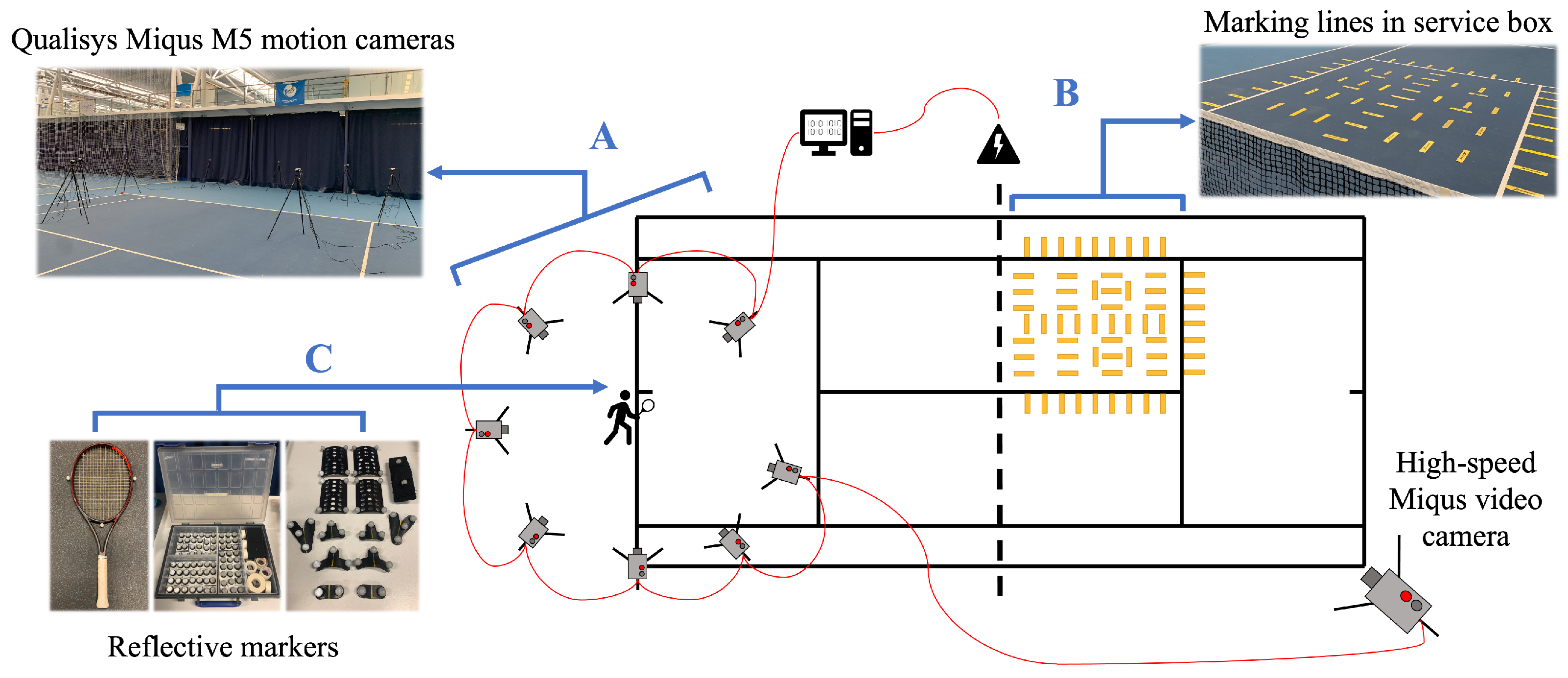
Figure 1. (A). Full indoor on-court experimental setup with Qualisys Miqus M5 motion cameras and a high-speed Miqus video camera. (B). 62 marking lines. (C). 75 individual markers.
Make 07 00118 g001
Figure 2. (a) A 45 degree motion capture camera still of player including computer setup. (b) Motion capture camera still from directly behind player including high-speed Miqus video camera (Qualisys, Gothenburg, Sweden).
Make 07 00118 g002
Figure 3. (a) Qualisys track manager trajectories for all 75 markers. (b) Long exposure from high-speed Miqus video camera showing ball trajectory from individual frames.
Make 07 00118 g003
Figure 4. Data inclusion/exclusion flow chart.
Make 07 00118 g004
Figure 5. Diagram of operation for Long Short-Term Memory models for classification of tennis serves.
Make 07 00118 g005
Figure 6. (a) Training and validation accuracy plots over 150 epochs for Stacked Bidirectional LSTM model. (b) Training and validation loss plots over 150 epochs for Stacked Bidirectional LSTM model.
Make 07 00118 g006
Figure 7. Diagram of operation for 3D Convolutional Neural Network for prediction of tennis serves.
Make 07 00118 g007
Figure 8. Training and validation mean squared error loss for 3D CNN model.
Make 07 00118 g008
Figure 9. (a) Normalised confusion matrix for classification of serves as “In”, “Out” and “Net”. (b) Actual and predicted coordinates for validation serves within a 4.1 m by 6.4 m service box over 20 runs.
Make 07 00118 g009
Table 1. Individual and total serve outcomes collected from participants during the experimental setup.
ParticipantInOutNetExcluded
111542153
211244163
Total22786316
Disclaimer/Publisher’s Note: The statements, opinions and data contained in all publications are solely those of the individual author(s) and contributor(s) and not of MDPI and/or the editor(s). MDPI and/or the editor(s) disclaim responsibility for any injury to people or property resulting from any ideas, methods, instructions or products referred to in the content.