Article

Enhancing Cancer Classification from RNA Sequencing Data Using Deep Learning and Explainable AI

Department of Computer Science, University College Cork, T12 XF62 Cork, Ireland
*
Authors to whom correspondence should be addressed.
Mach. Learn. Knowl. Extr. 2025, 7(4), 114; https://doi.org/10.3390/make7040114
Submission received: 18 July 2025 / Revised: 10 September 2025 / Accepted: 23 September 2025 / Published: 1 October 2025

Abstract

Cancer is one of the most deadly diseases, costing millions of lives and billions of USD every year. There are different ways to identify the biomarkers that can be used to detect cancer types and subtypes. RNA sequencing is steadily taking the lead as the method of choice due to its ability to access global gene expression in biological samples and facilitate more flexible methods and robust analyses. Numerous studies have employed artificial intelligence (AI) and specifically machine learning techniques to detect cancer in its early stages. However, most of the models provided are very specific to particular cancer types and do not generalize. This paper proposes a deep learning and explainable AI (XAI) combined approach to classifying cancer subtypes and a deep learning-based approach for the classification of cancer types using BARRA:CuRDa, an RNA-seq database with 17 datasets for seven cancer types. One architecture is designed to classify cancer subtypes with around 100% accuracy, precision, recall, F1 score, and G-Mean. This architecture outperforms the previous methodologies for all individual datasets. The second architecture is designed to classify multiple cancer types; it classifies eight types within the neighborhood of 87% of validation accuracy, precision, recall, F1 score, and G-Mean. Within the same process, we employ XAI, which identifies 99 genes out of 58,735 input genes that could be potential biomarkers for different cancer types. We also perform Pathway Enrichment Analysis and Visual Analysis to establish the significance and robustness of our methodology. The proposed methodology can classify cancer types and subtypes with robust results and can be extended to other cancer types.

1. Introduction

Cancer caused 10 million deaths in 2020, including 2.26 million breast cancer cases, 2.21 million lung cancer cases, 1.93 million rectum and colon cancer cases, 1.14 million prostate cancer cases, 1.09 million stomach cancer cases, and 1.20 million skin cancer cases [1,2]. Effective treatment and individualised therapy for cancer patients depend on early detection and correct diagnosis. Cancer detection and diagnosis rely heavily on morphological descriptors [3,4,5,6]. For instance, a pathologist uses a microscope for specific morphological features that are linked to breast cancer when a sample of breast tissue is obtained through a biopsy or surgical procedure [7,8]. These features include abnormal cell growth, changes in cell size or shape, and the presence of cancerous cells. These morphological traits can reveal crucial details regarding cancer’s type, stage, and aggressiveness, influencing therapy choices [9,10].
Despite its continued importance as a diagnostic and screening tool for cancer, morphological examinations have certain drawbacks [11,12,13,14]. Physicians may experience difficulties in identifying cases due to the limitations of morphological characteristics such as variability, overlapping, and low sensitivity in diagnosing and detecting cancer [15]. The emergence of Next-Generation Sequencing (NGS) and improvements in microarray technology have made patient gene expression profiling (GEP) more accessible. This has led to the creation of gene expression datasets related to different diseases. Personalized medicine has seen a dramatic change due to this move away from descriptive “morphological” classification methods toward a more all-encompassing approach that takes immunohistochemistry biomarkers and clinical features into account. GEP is already widely used in standard clinical practice [16,17]. Cancer researchers have thoroughly studied GEP, and clinical oncologists are beginning to incorporate the results of these investigations into their routine operations. Additionally, mining gene expression-level data has been beneficial for the early diagnosis and treatment of various cancer types [18]. Numerous techniques are developed based on information on gene expression to precisely forecast cancer [19,20,21]. As computer technology is developing quickly, computational methods are becoming increasingly important in detecting cancer. Using gene expression data, several machine learning, deep learning, and metaheuristic approaches have been developed and used to identify and categorize cancer.
Single- and dual-channel microarrays are being increasingly replaced by RNA-sequencing (RNA-seq) as the primary method used to assess gene expression profiles in biological investigations [22]. Depending on the chosen NGS technology and the RNA to be examined, RNAs of interest are isolated from a biological sample and an RNA fragment library is assembled. According to Hardlickova et al. [23] and Berge et al. [24], this stage typically entails the isolation of the RNA molecule, complementary DNA (cDNA) production by reverse transcriptase reaction, random amplification by polymerase chain reaction, and inclusion of sequencing adapters. There are several sequencing platforms, and their choice must consider the analysis procedure and the experiment aims since they exhibit varying performance [25,26,27]. Currently, Illumina is state-of-the-art, with its synthesis sequencing-based technology [28]. This method uses unique fluorescently tagged reversible terminator deoxyribonucleotide triphosphates (dNTPs), which are identifiable by the fluorescence color they generate [29]. Each cycle of dNTPs contains one nucleotide. While messenger RNA is the most researched type of RNA, other functional varieties are just as important to comprehend the cell’s regulatory apparatus, even if they do not code for proteins. RNA-seq stands out because it can select different RNAs, such as microRNA, long noncoding (lncRNA), and circular RNA, by varying RNA extraction and isolation protocols [30]. This enables the creation of unique protocols that extend beyond simply formulating probes to identify individual RNA types [31].
Due to this flexibility, businesses have invested in developing the technology, and as a result, RNA-seq investigations may now be carried out at prices that are competitive with microarray tests [32,33]. Consequently, it is anticipated that RNA-seq would present additional data-handling issues due to its completely distinct character from microarray results [34,35]. The first difficulty is the rigorous preprocessing necessary for precise analysis of RNA-seq. RNA-seq addresses read abundance as opposed to microarrays, which quantify the expression of a specific RNA in a biological sample through the appropriate hybridisation of cDNA with its probe [36,37,38]. It would be completely incorrect only to use the raw gene expression data as a result. In general, sample quality analysis, background correction, and normalization must be properly applied to a machine learning approach when working with microarray datasets [39]. However, in order to use RNA-seq, one must analyze the quality of the sample, eliminate low-quality bases, eliminate experimental artefacts, remove any remaining ribosomal RNA, estimate transcript-level abundance, and normalize RNA-seq read counts. Therefore, before implementing any AI methods, rigorous data processing must be performed. The second challenge lies in developing an algorithm capable of precisely examining such data.
With respect to the file input, RNA-seq raw data are given as non-negative elements and integer-valued counts rather than log-intensities like in the case of microarrays [34]. Therefore, it becomes essential to provide an input matrix that has undergone all preprocessing stages before the analysis stage provided by machine learning. Furthermore, the “curse of dimensionality”, which is linked to datasets with a large number of features but few samples, is very common in biological datasets [40]. This results in overfitting of the model, which impairs its generalization and increases computation times. Therefore, the development of more accurate algorithms is closely tied to the availability of high-quality data.
A detailed overview of recent cancer research efforts that use gene expression data from different cancer kinds was provided by Khalsan et al. [41]. The paper covers a number of applications of machine learning in cancer research, including the use of RNA-Seq and microarray data, cancer prediction and classification. Yuan et al. [42] used gene expression data to use several machine learning techniques for the identification of lung cancer. Wang et al. [43] presented a unique computational approach to diagnose breast cancer by combining Support Vector Machine (SVM) [44], dagging [45], rough set-based rule learning, Random Forest [46], and Monte Carlo Feature Selection [47]. Danaee et al. [48] introduced a deep learning technique that employs a Stacked Denoising Autoencoder (SDAE) to find genes that may successfully distinguish between tumor and healthy cases of breast cancer. Jia et al. [49] examined BRCA gene expression data from the Gene Expression Omnibus (GEO) [50] and The Cancer Genome Atlas (TCGA) [51]. They employed weighted gene co-expression network analysis (WGCNA) and differentially expressed genes to choose the most important genes. Alshareef et al. [52] suggested a deep learning model for prostate cancer detection in conjunction with an artificial intelligence-based feature selection approach (AIFSDL-PCD) utilizing gene expression data.
In recent years, notable advancements in cancer prediction have been witnessed using deep learning and machine learning techniques based on gene expression data. The performance of the current models is not without severe challenges. Selecting the ideal feature representation and architecture, which includes the number of layers and nodes, appropriate model parameters, and proper weight and bias values, is crucial in enhancing performance [53,54,55]. Furthermore, deciding on the best regularization parameters and learning rates can impact the model’s capacity to generalize to new data. To address these problems, this work seeks to develop the state-of-the-art use of a Convolutional Neural Network (CNN) for classifying gene expression data by identifying an accurate prediction model and employing metaheuristic techniques to optimize the CNN model. Optimization algorithms that repeatedly explore a vast search space and refine potential solutions are known as metaheuristic algorithms [56]. They can provide near-optimal solutions in a reasonable period of time for NP-hard problems, which are computationally intractable issues that cannot be solved with exact methods [57,58,59]. Meanwhile, large-scale bioinformatics optimization problems have been found to be effectively solved by metaheuristic optimization techniques. Since many of these issues fall under the NP-hard category, academics have mostly relied on metaheuristic approaches to solve them. Large-scale sample problems can be solved effectively with the use of metaheuristic techniques, which also minimize the need for computer resources. Although there are a variety of optimization techniques available, metaheuristic optimization algorithms are useful for resolving optimization issues because of their adaptability in producing superior optimization solutions in a very short processing time [60]. The challenges of high dimensionality, complicated variable correlations, and noisy data specific to gene expression data can all be solved with the use of metaheuristic models. Additionally, by utilizing strategies like randomization and simulated annealing to break out from local optima, metaheuristic models can manage noisy and non-linear data [61].
An artificial neural network-based metaheuristic approach for classifying skin diseases was presented by Chakraborty et al. [62]. In MotieGhader et al. [63], messenger RNA (mRNA) and micro-RNA expression data were utilized to identify breast cancer using a combination of SVM classifier and metaheuristic techniques such as genetic algorithm [64], world competitive contest [65], particle swarm optimization [66], cuckoo optimization [67], imperialist competitive algorithm [68], learning automata [69], heat transfer optimization algorithm [70], ant colony optimization [71], forest optimization algorithm [72], discrete symbiotic organisms search [73], and league championship algorithm [74]. As a result, the suggested algorithm chose 186 mRNAs out of 9692 and 116 miRNAs out of 489, which produced results with accuracy levels above 90% for the miRNAs dataset and 100% for the mRNA dataset. A generative adversarial (GANs) model on cancer genomic data was proposed by Wei et al. [75]. They employed twelve distinct gene expression datasets from the TCGA. Additionally, they employed a reconstruction loss to improve stability when training the model. Their suggested model obtained a 92.6% accuracy rate.
A two-stage gene selection model was presented by Deng et al. [76] for the categorization of cancer in microarray datasets. Their method coupled gradient boosting (XGBoost) with a multi-objective optimization genetic algorithm (XGBoost-MOGA). In the first step, a set of genes most pertinent to the class is left behind after irrelevant genes are efficiently ranked using XGBoost-based feature selection. In the second step, multi-objective optimisation with XGBoost-MOGA is used to identify a subset of optimal genes from the collection of the most relevant genes. A comparative study was conducted between the suggested method and other cutting-edge feature selection techniques, utilizing two commonly used learning classifiers on 14 publicly available microarray datasets. The outcomes showed that XGBoost-MOGA performed better than earlier techniques in terms of recall, accuracy, F-score, and precision.
Various other studies have focused on skin cancer classification using images employing deep learning and transfer learning [77,78,79,80] and XAI with breast and lung cancer data [81,82,83]. XAI refers to a set of tools and approaches meant to make the judgments and predictions of complex machine learning models more intelligible and interpretable to humans. Traditional AI models, especially deep learning models, typically function as “black boxes”, producing very accurate predictions without providing insight into how those predictions were formed. XAI seeks to overcome this gap by tracing the input that most influenced the outcome [84]. Local Interpretable Model Agnostic Explanation (LIME) [85] is a method in XAI to deliver human-understandable explanations for predictions made by deep learning models. In gene-based cancer classification, that equates to finding the most relevant genes that impact the classification.
By integrating the Barnacles Mating Optimizer (BMO) [86] algorithm with SVM, also known as BMO-SVM, Houssein et al. [87] were able to select genes that contribute to the prediction of cancer from gene expression datasets with the best accuracy based on microarray data. They assessed the suggested model using four benchmark microarray datasets: leukemia1, lymphoma, a small-round-blue-cell tumor (SRBCT), and leukemia2. According to their findings, the suggested BMO-SVM technique outperformed other well-known techniques, including genetic algorithm, Artificial Bee Colony [88], particle swarm optimization, and Tunicate Swarm Algorithm [89]. An approach for gene selection called the Improved Whale Optimization approach (IWOA) [90] was proposed by Devi et al. [91]. A multi-objective fitness function that strikes a balance between feature selection and error rate minimization was employed in the suggested approach. The findings demonstrate that the proposed method, which used the Gradient Boost Classifier to obtain a limited selection of genes needed for the BRCA classification, accomplished 97.7% accuracy. Similarly, Mohamed et al. [92] proposed a CNN architecture combined with EOSA to classify BRCA data from TCGA. They outperformed all the techniques mentioned above. Additionally, Jagadeeswararao et al. [93] used the SVM, KNN, and Logistic Regression to classify the pancreatic adenocarcinoma (PAAD) data from TCGA and achieved 96% accuracy. Wang et al. [94] used cfRNA data for the biomarker identification and cancer classification and, using RF and LR, achieved 90.5% Area Under the Curve (AUC).
One very important issue in RNA-seq data analysis is reliability and uniformity, as previously mentioned. In order to tackle that, Feltes et al. [95] proposed a dataset “BARRA:CuRDa”, which is made up of 17 carefully selected RNA-seq datasets for humans taken from the GEO and subjected to stringent filtering standards. Each dataset was subjected separately to analyses of sample quality, low-quality base removal, ribosomal RNA removal, experimental process artefacts, and transcript level abundance. The result is a curated RNA-seq dataset that works as a benchmark for human cancer classification experiments. The same work also used multiple machine learning algorithms, including Decision Tree [96], RF, k-nearest neighbors [97], multi-layer perceptron [98], and SVM to classify the cancer profiles. The comparison of all the above-mentioned studies is given in Table 1.
As summarized in Table 1, the criteria are defined as follows: sufficient data (SD) indicates that each cancer type or subtype has enough samples to allow reliable training and evaluation; single algorithm (SA) refers to the use of one consistent algorithm for a classification problem, as opposed to prior work that tested multiple algorithms such as SVM and Random Forest on the same dataset; domain-specific algorithms (DSAs) represent models customized or tuned for a specific cancer type; and multiple cancer types (MCTs) refers to models that simultaneously classify across different cancer types rather than focusing on a single cancer dataset. The main limitations of these studies include: most of them use TCGA Data, and in that, the comparison between conditions may be impacted by the fact that raw “fastq” normal samples are not publicly available for all institutions; the lack of public availability of raw “fastq” at TCGA hinders the ability to perform high-quality custom analysis and statistical treatments. Of critical importance, most studies use distinct algorithms, which perform differently for different datasets, suggesting that the results are hard to reproduce for new datasets of the same kind. Additionally, studies that use deep learning algorithms, although highly precise, do not usually output gene information, losing important biomarker information. A method that can handle different types of cancers without changing the methodology and parameters every time is much needed. Last but not least, they are focused on cancer subtype classification, not cancer type classification.
In this paper, we deal with these limitations by proposing a unified RNA-seq methodology for different cancer subtypes and a second deep learning-based algorithm for different cancer type classification, additionally producing an identification of relevant genes. First, we design a deep learning- and XAI-based lightweight model to classify cancer subtypes for multiple tissues and cancer types. This single model can be used for single- or multiple-class classification. Second, with the use of XAI, we could identify the gene information that impacted the classification result. These genes are potential biomarker candidates for cancer. For the cancer type classification, we develop another deep learning-based algorithm to classify the seven primary cancer types against one normal type. The major motivation behind developing a cancer type classifier is to identify the primary as well as metastatic cancer. While the cancer subtype classifier can help analyze the identified cancer types. We also analyze the 99 identified genes using the Kyoto Encyclopedia of Genes and Genomes (KEGG), Gene Ontology (GO), and visual analysis techniques to validate and demonstrate the robustness of our methodology. The visual analysis of the selected features also shows how well our methodology can handle the genes with high variance abundance values. The technical details of our methodology are given in the Methodology Section, while detailed results, our findings, results comparisons, and visual analyses are shown in the Results and Discussion Section.

2. Materials and Methods

This section describes the technical details of our methodology, including methods, equations, and illustrations. The summarized flow of our approach is shown in Figure 1.
The diagram shows the elements of the overall approach. Cancer subtype classification represents the classification within tissue type, e.g., normal or tumor profile classification; cancer type classification represents the overall classification, which is the classification of tissue types such as breast cancer or lung cancer. Each of the elements of the diagram is individually explained below.

2.1. Data Preprocessing

In our experiments, we employed the aforementioned RNA-seq database named BARRA:CuRDa [95]. We describe here the processes performed by the authors for completeness. They curated the dataset using the GEO query tool [101] for the R platform Version 4.3.1. Data for several cancer subtypes were obtained from the GEO database [50] to create numerous RNA-seq datasets named Geo Series (GSEs). Following data collection, a quality analysis was performed on the raw data for the selected datasets using the FastQC software [102]. Utilizing the Trimmomatic 0.35 tool [103], trimming was performed to eliminate low-quality bases, poly-N sequences, residual ribosomal RNA, and the sequences of adapters. The slidingwindow option was applied, in which each read was scanned with a window of four bases and trimming was performed once the average Phred quality score within that window dropped below 15. After trimming, the minlen option was applied to discard any read shorter than 65 bp. All datasets were processed using this procedure, except GSE6511, whose original read length was 40 bp. The data generated were aligned against the Homo sapiens reference sequence (Ensembl version GRCh38.94). Using the default parameters of the program, transcript-level abundance quantification was performed via aligning spliced transcripts to a reference (STAR) v2.6.0a [104] and RNA-Seq using expectation-maximization (RSEM) v1.3.1 [105]. The count data were converted utilizing variance stabilizing procedures from DESeq2 [106], and the outcomes were imported and summarized as matrices utilizing the tximport package [107].
The dataset has unbalanced and low numbers of profiles, discussed in Section 3.2. For the evaluation, data needed to be split into train and test sets, which further lowers the number of profiles for each set. To deal with this problem, we used the Synthetic Minority Over-sampling Technique (SMOTE) [108] (details in Section 2.2.1) on the training dataset to make sure the model can learn adequately and does not suffer from underfitting. While dealing with the cancer type classification, data were merged and reduced using Principal Component Analysis (PCA) [109] to reduce the number of parameters and make the model lightweight.

2.2. Cancer Classification

2.2.1. SMOTE for Synthetic Data Generation

SMOTE tackles class imbalance by generating synthetic samples for the minority class. Synthetic data points are generated by interpolating between a minority class instance and one of its k-nearest neighbors.
Minority Class Sampling
We let x i be a sample from the minority class. The set of its k-nearest neighbors, denoted as N k ( x i ) , is obtained by selecting the k points closest to x i in terms of Euclidean distance. This formula is represented mathematically as in Equation (1).
N k ( x i ) = { x j X { x i } x j is among the k closest samples to x i under x j x i }
where x j x i denotes the Euclidean distance between samples x i and x j .
Synthetic Point Generation
Once the nearest neighbors are determined, a synthetic sample x new is generated by linearly interpolating between x i and one of its neighbors x j . The generation formula is given as in Equation (2).
x new = x i + α ( x j x i ) , α ( 0 , 1 )
where α is a random number drawn from a uniform distribution.
Random State Control
To ensure reproducibility in the generation of synthetic samples, the value of α is drawn from a uniform distribution controlled by a random seed. This is defined as in Equation (3).
α U ( 0 , 1 )
where U ( 0 , 1 ) denotes the uniform distribution over the interval [ 0 , 1 ] .

2.2.2. Model for Cancer Subtype Classification

The model architecture is designed for both binary and multiclass classification using a one-dimensional CNN (Conv1D) [110]. The architecture can be divided into two parts: binary classification and multiclass classification. The key difference lies in the output layer, where sigmoid activation is used for binary classification and softmax activation is used for multiclass classification.
Convolution Operation
The model begins with a Conv1D layer, which applies a 1D convolution operation to the input data. Given an input sequence X R T × d , where T is the sequence length and d is the feature dimension, the convolution operation is defined as in Equation (4).
h t = f i = 1 d W i X t + i 1 + b i
where
  • h t is the output of the convolution at time step t,
  • W i is the kernel (filter) of the convolution for the ith feature,
  • X t + i 1 is the input at time step t + i 1 ,
  • b i is the bias term,
  • f ( · ) is the activation function, in this case, ReLU (Rectified Linear Unit).
Max-Pooling Operation
After the convolution, a max-pooling operation is performed to reduce the dimensionality and retain the most important features. The max-pooling operation can be written as in Equation (5),
p t = max ( h t : t + M 1 )
where M is the size of the pooling window and h represents the feature map from the previous layer.
Dropout
Dropout is performed to prevent overfitting by randomly changing a fraction p d r o p of input units to 0 at every update throughout training. Mathematically, dropout can be described as in Equation (6),
h drop = h r
where ⊙ denotes element-wise multiplication and  r Bernoulli ( p d r o p ) is a mask generated from a Bernoulli distribution with probability p d r o p .
Fully Connected Layers
After flattening the output of the max-pooling layer, the flattened vector is passed through one or more fully connected dense layers. The output of a dense layer is given by Equation (7),
z = f ( W h + b )
where
  • W is the weight matrix of the dense layer,
  • h is the input to the dense layer,
  • b is the bias vector,
  • f ( · ) is the activation function (ReLU for hidden layers).
Output Layer for Binary Classification
For binary classification, the output layer (given as dense_3 in Figure 2) contains a single unit with a sigmoid activation function, representing the probability of the positive class. The output is given by Equation (8),
y ^ = σ ( W h + b ) = 1 1 + e ( W h + b )
where σ ( · ) is the sigmoid activation function and b is the scalar bias associated with the output unit.
The binary cross-entropy loss function is used to optimize the model as in Equation (9),
L binary = y log ( y ^ ) + ( 1 y ) log ( 1 y ^ )
where y is the true label and y ^ is the predicted probability.
Output Layer for Multiclass Classification
For multiclass classification, the output layer (given as dense_3 in Figure 2) consists of C units (one for each class) with a softmax activation function as in Equation (10),
y ^ i = e z i j = 1 C e z j
where y ^ i is the predicted probability for class i, and  z i is the input to the softmax layer for class i.
The categorical cross-entropy loss function is used to optimize the model as in Equation (11),
L categorical = i = 1 C y i log ( y ^ i )
where y i is the true label (one-hot encoded) and y ^ i is the predicted probability for class i. The final model architecture for cancer-subtype classification is shown in Figure 2.

2.2.3. Early Stopping Criteria

An early stopping criterion is implemented to halt training once the validation accuracy reaches a target value. The stopping criterion can be described as in Equation (12),
Stop training if val _ accuracy target _ accuracy
A patience parameter P a t is used to determine how many epochs to wait after reaching the target accuracy before stopping. If the validation accuracy does not improve after P a t epochs, training is stopped.

2.3. Cancer Type Classification

As all our datasets are combined into one, the resulting dimensions are very large. We reduce the dimensions by employing PCA.

2.3.1. PCA on RNA Dataset

PCA is a dimensionality reduction technique that projects data from a high-dimensional space into a lower-dimensional subspace while preserving as much variance as possible. In the context of RNA sequencing data, which typically has tens of thousands of features (genes), applying PCA helps to reduce the dimensionality and capture the key patterns in the data.
For an RNA dataset with p features (genes), we let the input data matrix be X R n × p , where n is the number of samples and p is the number of genes. In our case, p = 58 , 735 , and n corresponds to the number of RNA samples. With  n _ c o m p o n e n t s = 640 , the dataset is projected into a 640-dimensional subspace. The mathematical details are outlined below.
Centring the Data
First, each feature (gene expression value) is centred by subtracting the mean of the feature across all samples as in Equation (13),
X centered = X μ
where μ R p is the vector of the mean values of each feature.
Covariance Matrix
The covariance matrix C R p × p is computed from the centered data matrix as in Equation (14),
C = 1 n 1 X centered X centered
The covariance matrix C captures the pairwise covariance between different genes.
Eigenvalue Decomposition
PCA involves computing the eigenvectors and eigenvalues of the covariance matrix C. The eigenvalue decomposition is as in Equation (15),
C = V Λ V
where
  • V R p × p is the matrix of eigenvectors (principal components),
  • Λ R p × p is the diagonal matrix of eigenvalues, where each eigenvalue represents the variance captured by its corresponding principal component.
Dimensionality Reduction
To reduce the dimensionality of the RNA-seq data to 640 components, the top 640 eigenvectors corresponding to the largest eigenvalues are selected. This forms the projection matrix V 640 R p × 640 , which is used to project the original data into the lower-dimensional space as in Equation (16),
X PCA = X centered V 640
where X PCA R n × 640 is the transformed data in the 640-dimensional subspace.
Variance Retained
The amount of variance retained by the top 640 principal components is proportional to the sum of the top 640 eigenvalues relative to the total sum of all eigenvalues, as in Equation (17),
Variance Retained = i = 1 640 λ i i = 1 p λ i
where λ i represents the eigenvalues in descending order.
Application in RNA Data
By applying PCA to the RNA-seq dataset with n _ c o m p o n e n t s = 640 , we reduce the original dataset from 58,735 dimensions (genes) to 640 dimensions while retaining most of the dataset’s variance. This procedure reduces the complexity of the model and helps prevent overfitting when used for classification tasks [112].
In our deep learning models, the PCA-transformed data can be used as input to improve the model’s performance by focusing on the most significant components of the gene expression data. Additionally, PCA facilitates visualizations and downstream analyses by simplifying the data to a more manageable number of dimensions.

2.3.2. Model for Cancer Type Classification

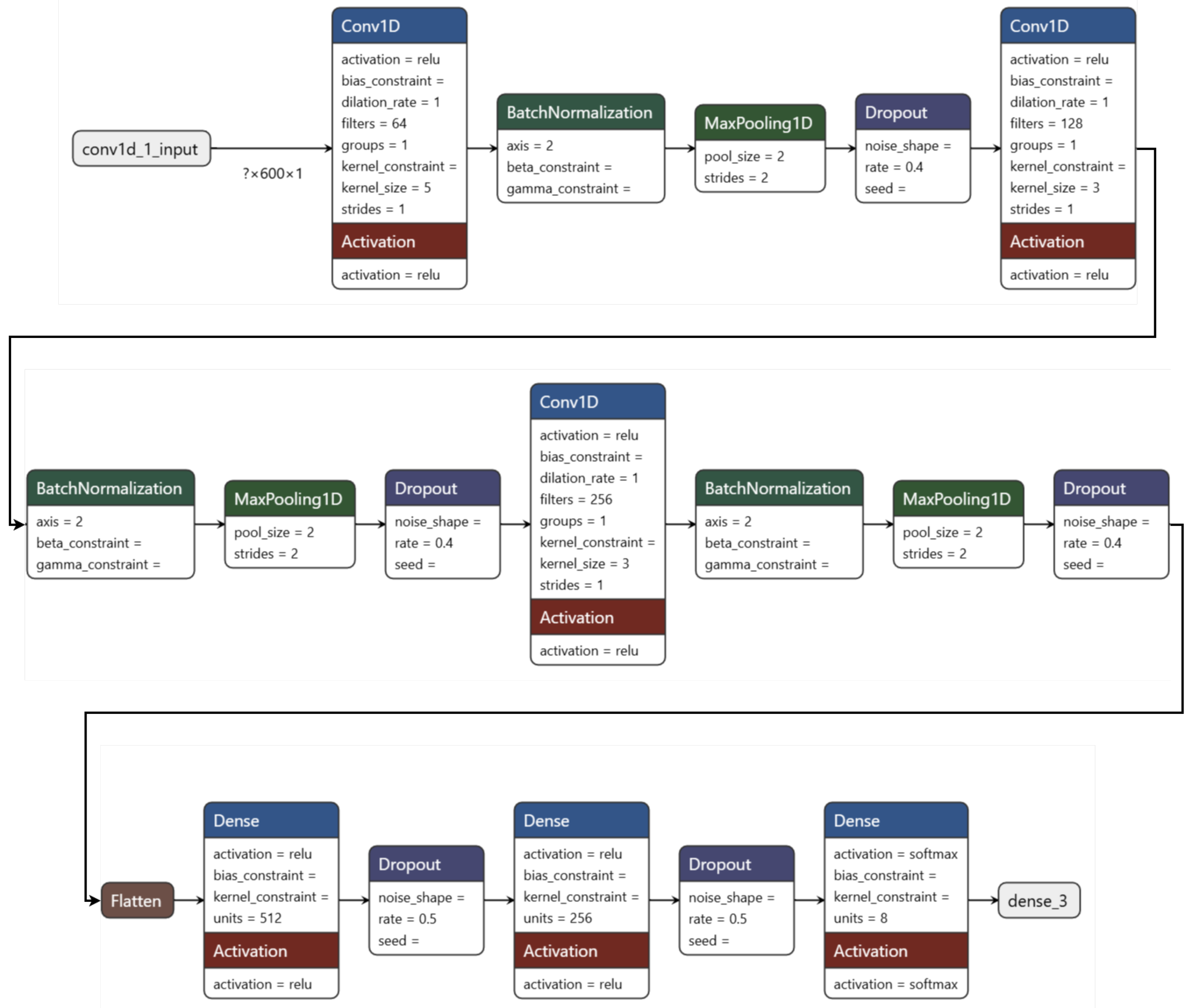
This subsection describes the architecture and mathematical formulation for the CNN used for multiclass cancer type classification of RNA sequencing data. The architecture consists of three convolutional layers, followed by batch normalization, max pooling, dropout layers, and dense layers. The AdamW optimizer is used to minimize the categorical cross-entropy loss. The model leverages regularization techniques such as L2 weight regularization, dropout, and learning rate adjustments to improve generalization. The visual representation of the model architecture for the cancer-type classification is shown in Figure 3.
The model is trained on input data X R n × p f e a t _ a f t e r × 1 , where n is the number of samples, p f e a t _ a f t e r is the number of features after dimensionality reduction, and the input has a single channel since the data are univariate.
First Convolutional Layer
-
The first layer applies a 1D convolution to the input as in Equation (18),
Z 1 = ReLU ( X W 1 + b 1 )
where ∗ represents the convolution operation, W 1 R 5 × 1 × 64 are the filters (64 filters of size 5), and  b 1 R 64 is the bias term. A regularization term is added using L2 regularization as in Equation (19),
L reg ( W 1 ) = λ 2 W 1 2
where λ = 0.01 is the L2 regularization parameter.
Batch Normalization
-
Batch normalization is applied to normalize the activations as in Equation (20),
Z 1 norm = Z 1 μ B σ B 2 + ϵ γ + β
where μ B and σ B 2 are the batch mean and variance, ϵ is a small constant to prevent division by zero, and  γ and β are learnable parameters.
Max Pooling
-
Max pooling is used to reduce the spatial dimensions of the output as in Equation (21),
Z 1 pool = max ( Z 1 norm , pool _ size = 2 )
Dropout
-
Dropout is applied to prevent overfitting by randomly setting 50% of the activations to zero as in Equation (22),
Z 1 drop = Z 1 pool r 1
where ⊙ represents element-wise multiplication and r 1 Bernoulli ( 0.5 ) .
Second and Third Convolutional Layers
-
The second and third convolutional layers are applied similarly to the first layer, with the following transformations as in Equation (23),
Z 2 = ReLU ( Z 1 drop W 2 + b 2 ) , Z 3 = ReLU ( Z 2 drop W 3 + b 3 )
where W 2 R 3 × 64 × 128 and W 3 R 3 × 128 × 256 , and batch normalization, max pooling, and dropout are applied after each layer.
Flattening Layer
-
After the last convolutional layer, the output is flattened into a 1D vector as in Equation (24),
Z flat = Flatten ( Z 3 drop )
This transformation prepares the data for fully connected layers.
Fully Connected Layers
-
Two fully connected layers are applied, each with ReLU activation and L2 regularization as in Equation (25),
Z dense 1 = ReLU ( Z flat W 4 + b 4 ) , Z dense 2 = ReLU ( Z dense 1 W 5 + b 5 )
where W 4 R d flat × 512 and W 5 R 512 × 256 , and dropout is applied after each layer as in Equation (26),
Z dense 1 drop = Z dense 1 r 4 , Z dense 2 drop = Z dense 2 r 5
Output Layer
-
The final dense layer (given as dense_3 in Figure 3) produces the class scores with softmax activation as in Equation (27),
y ^ = softmax ( Z dense 2 drop W 6 + b 6 )
where W 6 R 256 × c and c is the number of classes. The softmax function ensures that the output is a valid probability distribution as in Equation (28),
y ^ i = exp ( Z i ) j = 1 c exp ( Z j ) , i { 1 , , c }
The final model architecture for cancer-type classification is shown in Figure 3.

2.3.3. Optimization and Class Balancing

To address class imbalance during training, class weights are computed and used to adjust the loss function. These weights ensure the model gives appropriate importance to each class, especially the minority classes.
Computation of Class Weights
We let C = { c 1 , c 2 , , c k } be the set of k classes, where n i denotes the number of samples in class c i , and N is the total number of samples in the training set as in Equation (29),
N = i = 1 k n i
The frequency f i of each class c i is calculated as in Equation (30),
f i = n i N
The class weight w i for each class c i is computed as in Equation (31),
w i = 1 f i j = 1 k 1 f j · k
The computed class weights are used to adjust the loss function during training.
Loss Function with Class Weights
The categorical cross-entropy loss function with class weights is defined as in Equation (32),
L weighted = i = 1 k w i · y i · log ( y ^ i )
where
  • w i is the weight for class c i ,
  • y i is the true label for class c i (one-hot encoded),
  • y ^ i is the predicted probability for class c i .
Optimization
The model is optimized using the AdamW optimizer, which is an Adam optimizer with decoupled weight decay as in Equation (33),
W t + 1 = W t η m ^ t v ^ t + ϵ + λ W t
where m ^ t and v ^ t are the biased-corrected first and second moment estimates, η is the learning rate, and  λ is the weight decay parameter.
Regularization
L2 regularization is applied to the weights in the convolutional and dense layers to prevent overfitting. The regularization term is added to the loss function as in Equation (34),
L reg = λ 2 W 2
Callbacks
The early stopping criteria are designed to stop the training when the validation loss does not improve for 20 epochs. The model’s weights are saved when the validation loss improves in the model checkpoints. The learning rate is reduced by a factor of 0.5 if the validation loss does not improve for five consecutive epochs, with a minimum learning rate of 10 6 .
Training
An 80:20 ratio was used to divide the dataset into training and testing sets; the testing portion was further split using a 50:50 ratio to create distinct validation and test sets, which were stratified by class labels. The model is trained for 500 epochs with a batch size of 32 using class weights to handle class imbalance in the RNA data. The history of the training and validation metrics is stored for analysis.

2.4. Explainability and Visual Analysis

2.4.1. XAI Using LIME

LIME is a method that explains the predictions of a complex, black-box model by approximating it with an interpretable model in the local neighborhood of the instance being explained. In our case, LIME is used to interpret the predictions of the RNA-seq deep learning model.
The core idea of LIME is to fit a local surrogate model g around the prediction of the complex model f for a specific instance x. The surrogate model is trained on perturbations of the original instance, weighted by their proximity to x.
We let f : R d R K represent the complex model, where d is the number of features (genes) and K is the number of classes. The model outputs the predicted probabilities f ( x ) for a given input x.
For a given instance x, LIME generates perturbed samples { x 1 , x 2 , , x N } from the original instance by altering some of its feature values. The corresponding predictions f ( x i ) are recorded, and the proximity π x ( x i ) of each perturbed sample to the original instance x is computed using a kernel function, such as the exponential kernel as in Equation (35),
π x ( x i ) = exp d ( x , x i ) 2 σ 2
where
  • d ( x , x i ) is the distance between the original instance x and the perturbed instance x i (e.g., using Euclidean distance),
  • σ controls the width of the kernel and the locality of the explanation.
Next, a simply interpretable model g ( x ) , such as a linear model, is trained on the perturbed data weighted by their proximity to x. The objective is to minimize the following weighted loss function as in Equation (36),
L ( f , g , π x ) = i = 1 N π x ( x i ) f ( x i ) g ( x i ) 2 + λ · Ω ( g )
where
  • f ( x i ) is the prediction of the original complex model on the perturbed instance x i ,
  • g ( x i ) is the prediction of the surrogate model on x i ,
  • π x ( x i ) is the proximity weighting,
  • Ω ( g ) is a regularization term that controls the complexity of the surrogate model g,
  • λ is a hyperparameter that controls the regularization strength.
Feature Importance
The LIME explanation provides a list of feature importance values w i , where each feature i contributes to the local decision. These weights represent the contribution of each gene i to the prediction for the instance x as in Equation (37),
g ( x ) = w 0 + i = 1 d w i · x i
where w i is the weight assigned to gene i and x i is the feature value of gene i for the instance x.
Application to RNA Data
By applying LIME to our deep learning model trained on RNA-seq data, we can extract the most important genes contributing to the prediction for a given sample. This extraction enables us to identify which genes drive the classification decisions, adding interpretability to the model.
The extracted feature importance values were subsequently used to generate plots, demonstrating the robustness of the model. The heatmaps, cluster maps, and violin plots were generated based on the genes identified as important by LIME, allowing for further validation of the model’s behavior. Visualizations can then be used to gain insight into the main features (genes) that led to the results.

2.4.2. Heatmap

A heatmap is a data visualization technique that represents the values of a matrix as colors. In the context of RNA data, the rows can represent genes, and the columns can represent different samples or conditions. Each cell H i j in the heatmap corresponds to the expression value of gene i in sample j, where colors represent the magnitude of the expression values.
Mathematically, the heatmap is based on a matrix H R m × n , where m is the number of genes and n is the number of samples. Each element H i j represents the value of GE, and it can be normalized using methods such as z-score normalization as in Equation (38),
Z i j = H i j μ i σ i
where
  • H i j is the expression value of gene i in sample j,
  • μ i is the mean expression value of gene i across all samples,
  • σ i is the standard deviation of gene i across all samples.
The heatmap provides an immediate visual insight into the patterns of gene expression across samples, which can be used to observe clusters or correlations within the RNA data.

2.4.3. Cluster Map

A cluster map extends the heatmap by incorporating hierarchical clustering. It clusters both rows (genes) and columns (samples) based on similarity, allowing for better pattern detection in RNA data. The clustering is often performed using the Euclidean distance d ( x , y ) between two vectors x and y , where each vector represents either a gene’s expression profile or a sample’s expression across genes as in Equation (39).
d ( x , y ) = i = 1 n ( x i y i ) 2
To create the hierarchical tree, a linkage method such as “average” linkage or “complete” linkage is applied. The linkage function L can be written as in Equation (40),
L ( A , B ) = 1 | A | | B | x A y B d ( x , y )
where A and B are clusters and  d ( x , y ) is the distance between elements x and y.
The cluster map helps reveal patterns such as co-expressed gene clusters or sample similarity, demonstrating the robustness of the model’s classification on RNA data.

2.4.4. UMAP (Uniform Manifold Approximation and Projection)

UMAP is a dimensionality reduction technique used to project high-dimensional RNA data into a lower-dimensional space while preserving its global and local structure. We let X R m × d represent the RNA data, where m is the number of samples, and d is the number of features (genes). UMAP projects X into a lower-dimensional space Y R m × 2 or Y R m × 3 .
UMAP relies on a weighted k-nearest neighbor (k-NN) graph. The weight w i j between two points x i and x j is computed using the probability distribution based on local distances as in Equation (41),
w i j = exp d ( x i , x j ) ρ i σ i
where
  • d ( x i , x j ) is the distance between points x i and x j ,
  • ρ i is the distance to the nearest neighbor of x i ,
  • σ i is a normalization factor.
The low-dimensional projection is then optimized to preserve both local and global structures by minimizing the cross-entropy between the original high-dimensional graph and the low-dimensional embedding.
UMAP is particularly useful in showing how well a dataset clusters by class, providing insights into the model’s performance in segregating biological samples.

2.4.5. Violin Plot

A violin plot is a method of plotting numeric data and comparing distributions. It is similar to a box plot, but it includes a kernel density estimate (KDE) of the data’s probability density. For RNA data, a violin plot is useful to visualize the distribution of gene expression levels across different conditions or classes.
Given a set of expression values X = { x 1 , x 2 , , x n } , the KDE is defined as in Equation (42),
f ( x ) = 1 n h i = 1 n K x x i h
where
  • K ( · ) is the kernel function (often Gaussian),
  • h is the bandwidth parameter,
  • n is the number of data points.
The violin plot shows the KDE on both sides of the central line, making it easier to see the density and distribution of RNA expression levels. It helps demonstrate the robustness of the model by visually comparing the spread of gene expression data across different classification results or labeled conditions.

2.5. KEGG Pathway Enrichment Analysis

To complete our analysis and find physiologically relevant pathways, we performed a KEGG pathway enrichment analysis using the clusterProfiler [113] package in R. Finding over-represented pathways based on differentially expressed genes in the dataset was the aim of the investigation. The following measures were implemented.
Gene Selection:
Differentially expressed genes were extracted using the RNA-seq dataset. The AnnotationDbi and org.Hs.eg.db packages were utilized to map Entrez IDs [114] to gene identifiers. In order to preserve alignment with the KEGG database, only genes with a valid Entrez ID were used for further analysis.
Pathway Enrichment:
The KEGG pathway enrichment was performed using the enrichKEGG function of the clusterProfiler package. The gene list, which contained the Entrez IDs of the differentially expressed genes, served as the input to the process. The parameters selected for the enrichment analysis were as follows:
  • Organism: Homo sapiens, symbolized by “hsa” in KEGG.
  • p-value Adjustment Method: Multiple comparisons were accounted for by applying the Benjamini–Hochberg (BH) method. This method is recommended for high-throughput analyses, such as RNA-seq, because it controls the false discovery rate (FDR).
  • q-value Cut-off: A strict q-value threshold of 0.05 was applied to ensure that only highly enriched pathways were retained. Pathways with a q-value greater than 0.05 were considered non-significant and excluded from further analysis.

2.6. GO Enrichment Analysis

The enrichGO function from the clusterProfiler package was used for GO enrichment analysis. The gene list was used as input, and the following settings were applied:
  • Organism: Homo sapiens (symbolized as ’hsa’).
  • p-value adjustment method: Benjamini–Hochberg (BH) to control the false discovery rate (FDR).
  • Threshold: Significant GO keywords were found with a p-adjusted value ( p . a d j u s t ) below 0.05.

Equations for p-Value Adjustment

The p-values were modified using the Benjamini–Hochberg (BH) approach to control the FDR. The adjusted p-values ( p a d j ) were computed using Equation (43),
p a d j = p · N r a n k ( p )
where
  • p is the original p-value,
  • N is the total number of tests,
  • r a n k ( p ) is the rank of the p-value among all tests.

3. Results and Discussion

In this section, we present the setup of our experiments and analyze the results.

3.1. Experimental Setup

These experiments were performed using the 13th-generation Intel Core i9-13900k (32 CPUs) (Santa Clara, CA, USA), 64 GB RAM, and NVIDIA A100-PCIE Graphical Processing Unit (Santa Clara, CA, USA). Due to the high dimension of data, the number of parameters in the model was high and required high computational power to train the model. The model architectures are shown in Figure 2 and Figure 3. We used Python 3.9.18 and TensorFlow 2.10.1 to perform these experiments.

3.2. Dataset Description

The dataset [95] contains seven types of cancers that include Breast, Colon, Head/Neck, Kidney, Liver, Prostate, and Lung. There are 17 tissues included in the dataset, and for each tissue, there are 58735 genes besides Colon_SRR2089755 and Colon_GSE50760, as these have 58,148 genes. The Colon_GSE50760 has three types of profiles, including Primary, Normal, and Metastasis, and Colon_SR2089755 has four types of profiles, including NormalColon, NormalLiver, Primary, and Metastasis. All other 15 cases have two types of profiles, including Normal and Tumor. Detailed information about the dataset is given in Table 2.
We did not need to merge datasets for the cancer subtype classification task, as each dataset was used individually. For the cancer type classification task, however, we merged the 17 RNA-seq datasets into a single dataset. Since the subtype and merged type datasets have different numbers of features, we applied padding to align them for model training. As a result of merging, our final dataset shape was transformed to 640 instances with 58,735 features.

3.3. Evaluation Measures

We used the following measures to evaluate the performance of our methodology for cancer classification using RNA data.
Accuracy: The proportion of correctly classified cancer and healthy samples out of the total number of RNA samples, as in Equation (44):
Accuracy = TP + TN TP + TN + FP + FN
Precision: The proportion of correctly identified cancer samples among all samples classified as cancer, as in Equation (45):
Precision = TP TP + FP
Recall: The proportion of actual cancer samples that were correctly identified by the model, as in Equation (46):
Recall = TP TP + FN
F1 Score: The harmonic mean of precision and recall, as in Equation (47):
F 1 Score = 2 · Precision · Recall Precision + Recall
Geometric Mean (G-Mean): Evaluates the balance between sensitivity and specificity, as in Equation (48):
G - Mean = Sensitivity · Specificity
where
Sensitivity = TP TP + FN
and
Specificity = TN TN + FP
where
  • TP = Number of correctly classified cancer samples,
  • TN = Number of correctly classified healthy samples,
  • FP = Number of misclassified cancer samples as healthy,
  • FN = Number of misclassified healthy samples as cancer.

3.4. Robustness of Our Methodology

The architecture that we employed for classifying RNA-seq data is based on a 1D CNN (Conv1D) specifically built to handle the sequential nature of gene expression data. Conv1D layers are ideal for RNA-seq data, where the gene expression levels matter because they are especially good at extracting localized patterns from data. The model detects subtle but substantial gene expression connections by applying convolutional filters throughout the input. These dependencies may be correlated with biological aspects like co-expressed genes or pathways implicated in disease processes. By adding a MaxPooling1D layer, the dimensionality of the data is reduced while the most important features are retained. This controls overfitting, which is a common problem when working with high-dimensional RNA-seq datasets and increases the computational efficiency of the model.
Dropout layers, which randomly deactivate a percentage of the neurons during training and force the model to generalize rather than rely on specific neurons, are essential to the robustness of the model. Considering that most RNA-seq research has limited sample sizes, this regularization technique is crucial. Furthermore, the AdamW optimizer was selected because, in contrast to conventional gradient descent, it enables the model to converge more rapidly and consistently. This is because of its adjustable learning rates. With slight changes, the model’s architecture can handle problems involving both binary and multiclass categorization. The output layer uses a softmax activation function for multiclass classification and a sigmoid activation function for binary classification. Because of its versatility, we show that the same base model may be applied to a larger variety of RNA-seq datasets and effectively handle different categorization tasks.
In summary, our CNN-based model design successfully balances efficiency and complexity. Convolutional layers, max pooling, dropout, and fully connected layers work together to minimize overfitting and guarantee that the model extracts both high- and low-level characteristics from the RNA-seq data. When dealing with RNA-seq data, which frequently has a small sample size but a high number of features (genes), this method works especially well. Furthermore, the architecture is a very solid option for applications like cancer classification, where it is crucial to identify minute differences in gene expression. This is because it can extract biologically significant patterns from the data, employing regularization techniques and a robust optimizer.
However, for the cancer-type classification, by adding more convolutional layers, more regularization methods, and deeper learning layers to the basic Conv1D architecture, the model improves further, making it suitable to handle complex multiclass classification tasks with RNA-seq data. The network can gradually capture more complex and high-level characteristics thanks to the model’s incorporation of three Conv1D layers with progressively larger filter sizes (64, 128, and 256). Batch normalization is used in conjunction with each convolutional layer to standardize activations and hasten convergence while stabilizing training. Large weight values are penalized by L2 regularization, which is performed on both convolutional and dense layers to prevent overfitting. In order to further reduce dimensionality, MaxPooling1D layers trail each convolutional block, and Dropout layers, which randomly remove neurons during training, guarantee additional regularization.
The model uses two dense layers (512 and 256 units) with ReLU activations to analyze high-level features learned by the convolutional layers. The last dense layer has a softmax activation function, making it perfect for multiclass classification, where it outputs the probability of each cancer kind. Weight decay is incorporated into the AdamW optimizer, which speeds up learning and enhances the model’s generalization. In order to prevent overfitting, early stopping and ReduceLROnPlateau are used to ensure training ends when validation performance stagnates.
Class weights are also applied during training to account for any possible class imbalance in the dataset and make sure the model did not miss any less common kinds of cancer. To better balance the distribution of classes, resampling the training data was added. With these improvements, the model becomes more resilient and can handle the intricacies of classifying cancer types by utilising the capabilities of deep CNN, sophisticated regularisation, and reliable optimisation methods. The reason behind using two different architectures is to keep the methodology lightweight. The first model for cancer subtype classification is quite light and can handle data with binary and multiple classes. The second model has more parameters and is used to classify the multiple types of cancers.
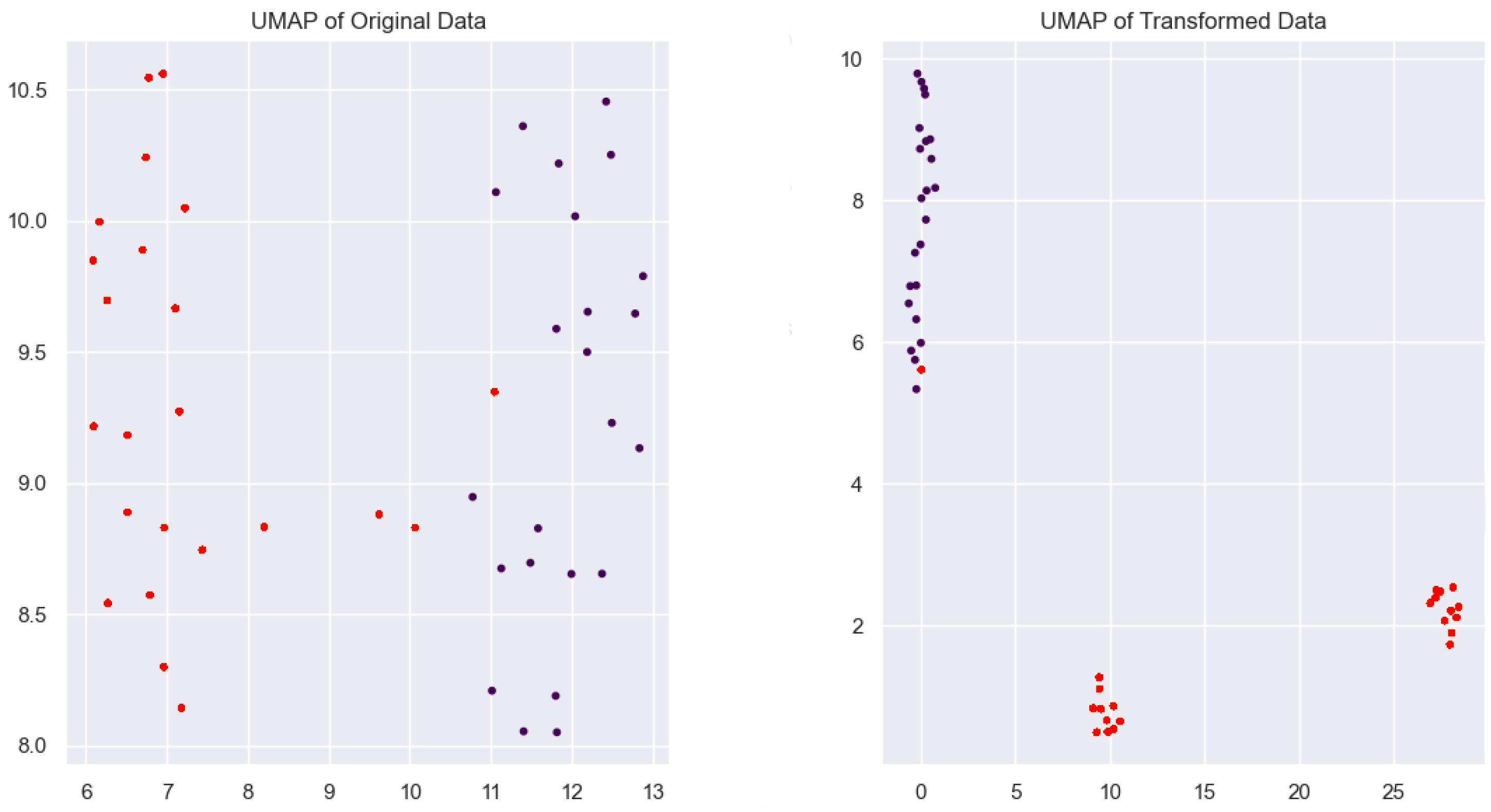
Due to space limitations, it was not feasible to present all datasets in detail. We therefore randomly selected the lung tissue dataset GSE87340 as a binary class and colon tissue SRR2089755 as a multiclass representative example to illustrate the workflow and results. Furthermore, the selection of these tissues shows the robustness of our methodology on linear and non-linear distributed data. For example, Figure 4 shows clear separation between two classes (tumor vs. normal), while additional figures, including Figure 9 for cancer subtypes and Figure 13 for cancer type classification, illustrate cases involving more complex, multi-class and non-linear distributions. The results of our model for the binary class for tissue GSE87340 are shown in Figure 5. The curves shown represent the accuracy and loss over epochs. The number of epochs was fixed at 200, but due to early stopping criteria, training stops automatically at different numbers of epochs. The best weights are saved to ensure the top accuracy achieved by our model, which is 100% for all datasets in the cancer classification task.
The separation of data points performed by our model for the tissue GSE87340 is shown in Figure 4. In these images, the normal profiles are represented in red, while other colors represent tumor profiles. These graphs show the capability of our methodology to separate the profiles regardless of the number and random distribution. These images show that our methodology is robust enough to handle linear and non-linear distributions of data.
The abundance values of top genes for the tissue GSE87340 are shown in Figure 6. These figures show the power of our methodology to handle high variance, outliers, and uneven distribution of data, all common in the identification and quantification of genes.
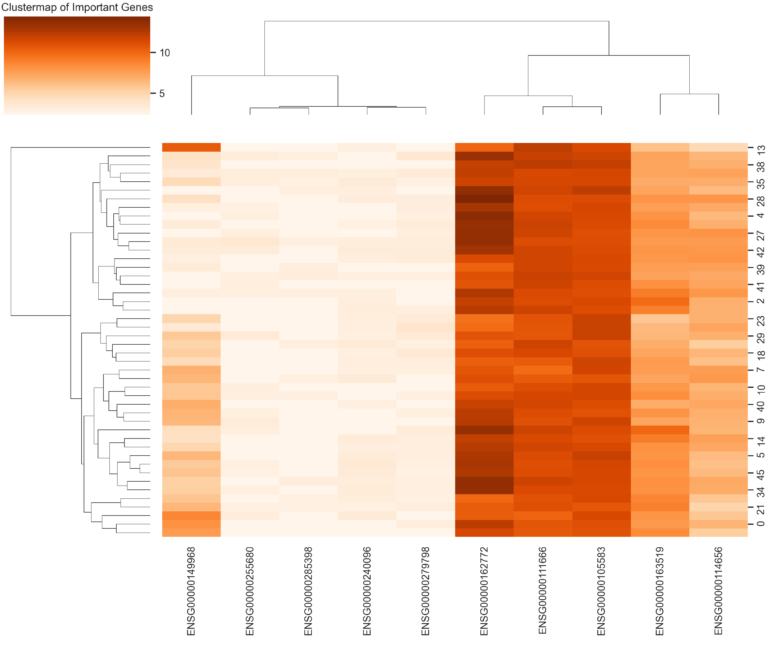
The cluster map of top genes for the tissue GSE87340 is shown in Figure 7. These images show the classification robustness of our model with mixed kinds of correlation. Genes clustered together exhibit similar expression patterns (positive correlation), while separation into distinct branches reflects weak or negative correlations. Our methodology highlights the genes with high correlation and those with low correlation; our model classifies based on mixed features, which makes it more reliable.
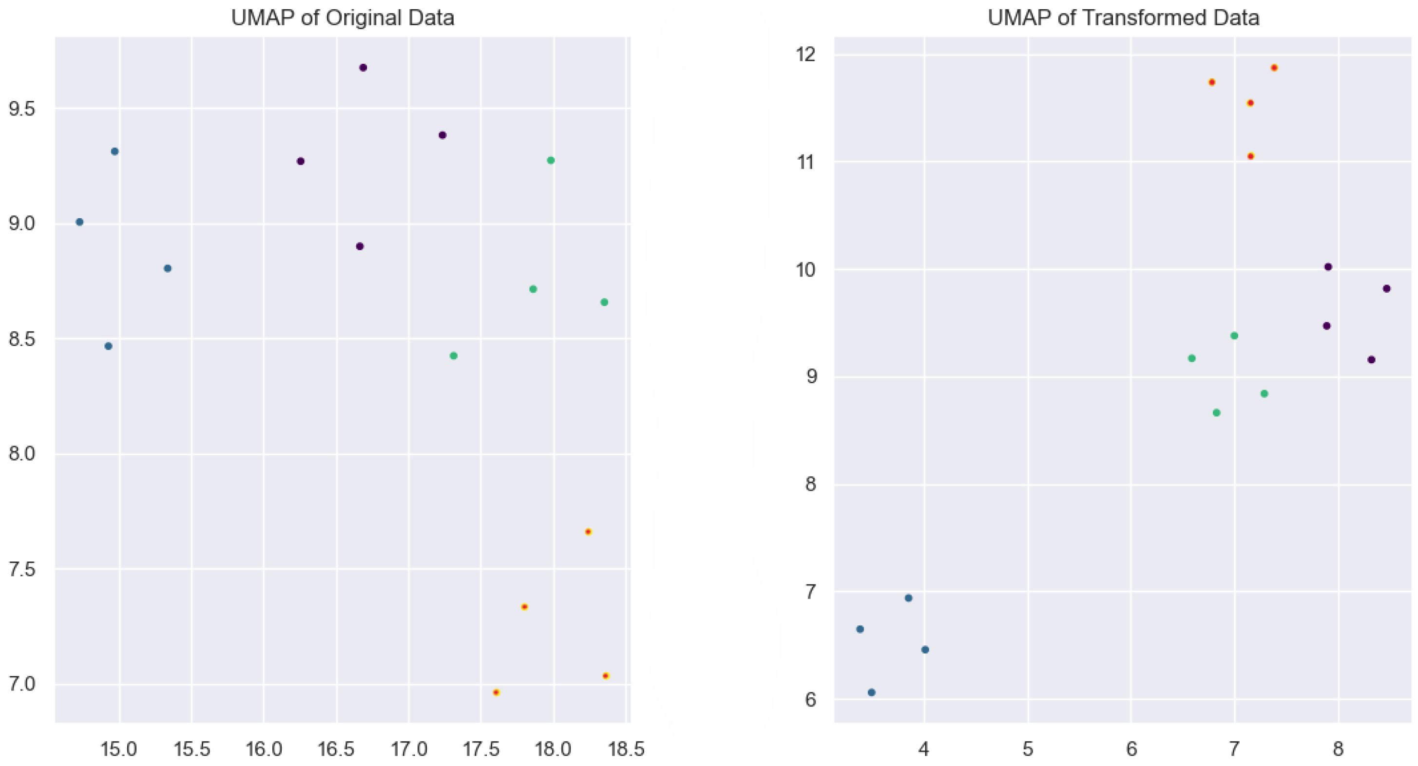
The results of our model for the four classes of tissue SRR2089755 are shown in Figure 8. The separation of data points performed by our model for the tissue SRR2089755 is shown in Figure 9. The abundance values of top genes for tissue SRR2089755 are shown in Figure 10. The cluster map of top genes for tissue SRR2089755 is shown in Figure 11.
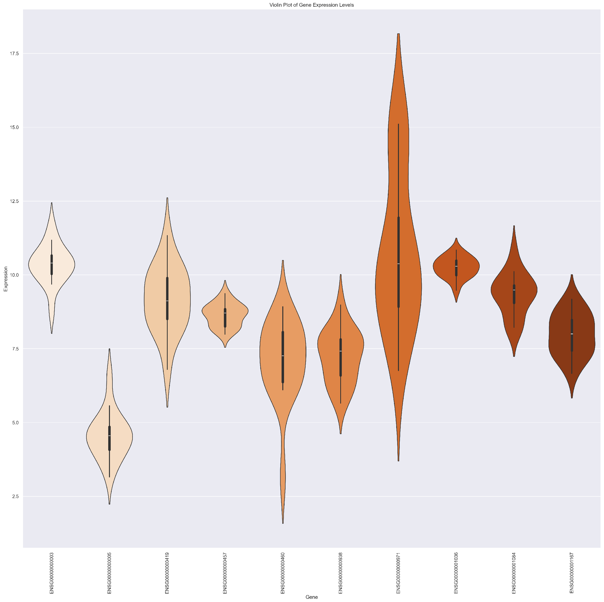
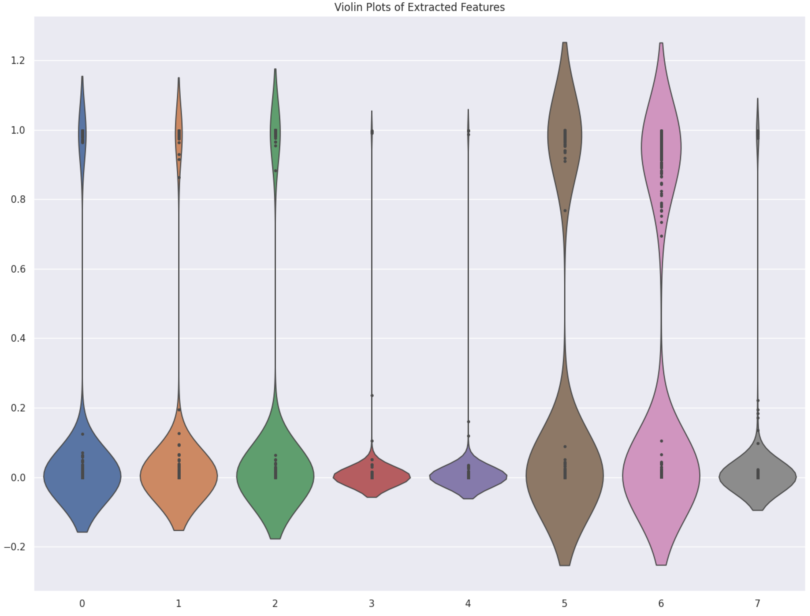
The violin plot for gene expression levels provides a good representation of the distribution of expression values across a range of genes. The ample range in the shapes of the violins implies that the model is excellent at capturing both highly variable and smoother gene expression patterns. The various violin shapes across different genes, as well as the spread of expression values, support the model’s capacity to discriminate across gene expression levels, which is critical for discovering cancer-specific biomarkers. The robust performance of the model in this image indicates its capacity to generalize across varied gene expression patterns while maintaining sensitivity to essential features, supporting its success in cancer classification tasks.
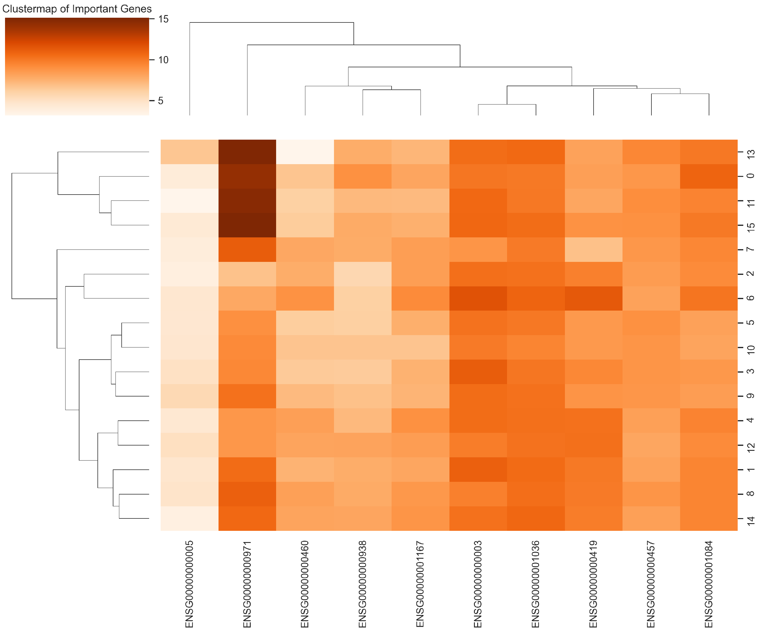
The shown cluster map gives a strong representation of the hierarchical clustering of genes based on their expression patterns, demonstrating key links between gene clusters. The obvious clusters of related genes illustrate the model’s robustness in finding patterns of gene co-expression. This robustness is especially relevant for cancer classification, as co-expressed genes generally lead to shared biological processes or pathways. The hierarchical structure in the dendrogram further highlights the model’s ability to recognize complex interactions between genes. This level of deep clustering verifies the model’s capacity to not only classify cancer kinds but also provide biological insights, particularly in the discovery of genes or gene sets that may operate as cancer biomarkers.
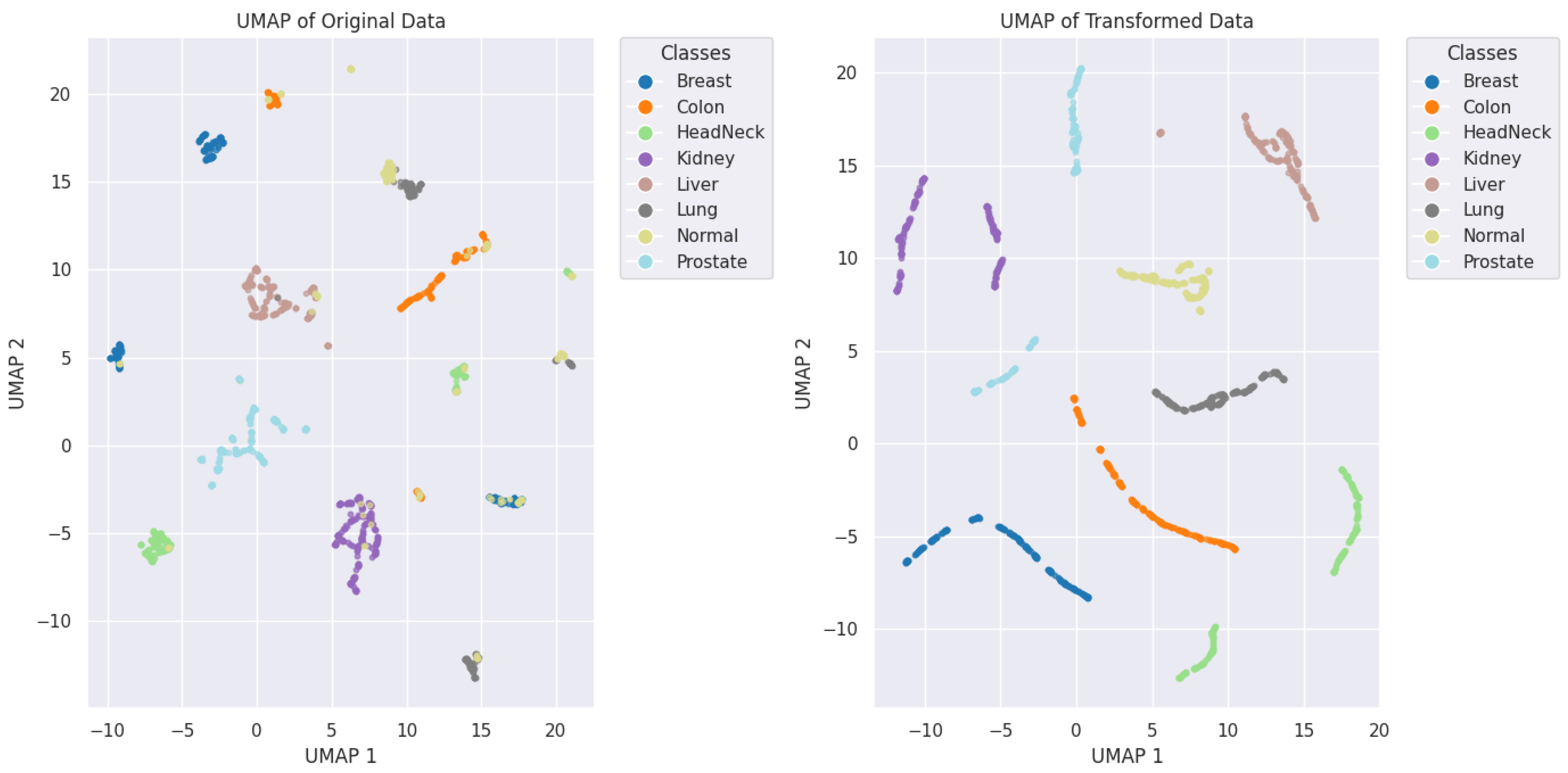
The results of our model for cancer type classification (eight classes) are shown in Figure 12. The separation of data points performed by our model for eight classes is shown in Figure 13.
The violin plot for cancer-type classification shows the distribution of extracted characteristics, illustrating how effectively the model captures essential properties from the RNA-seq data. The variety in the shape and size of the violins for different extracted data illustrates the model’s capacity to catch distinct patterns across various cancer types. Some violins are significantly wider, showing a vast range of feature values that may correspond to diverse biological properties within cancer types. This diversity further confirms the model’s robustness in retrieving and learning from the data, ensuring that it does not miss details that could be important for successful categorisation. The evident separations between the different extracted characteristics further underscore the model’s capacity to generalize across numerous classes while maintaining performance across varied inputs.
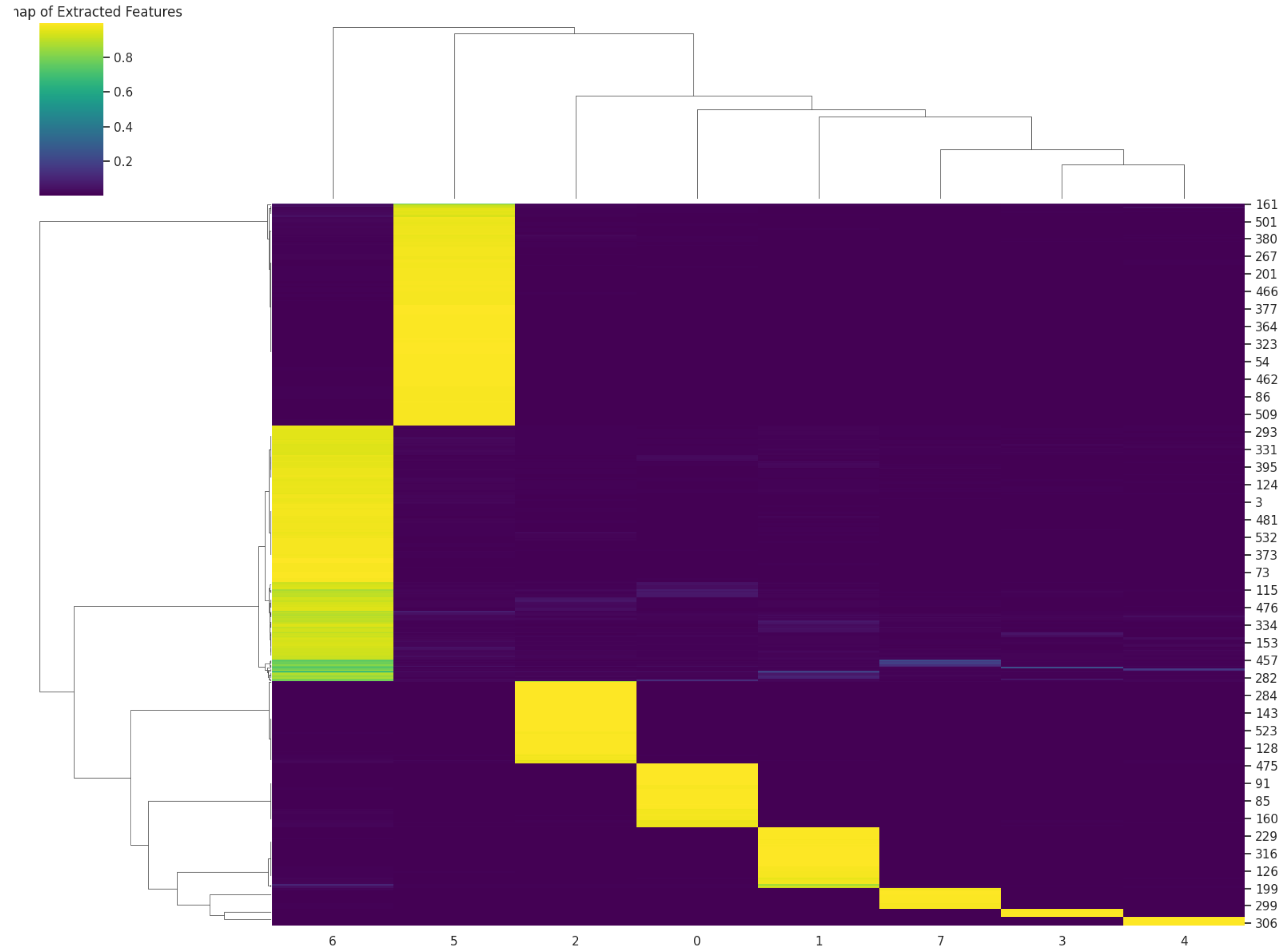
The heatmap visualization highlights the retrieved features and demonstrates a clear clustering of features that are strongly connected. The color variations that extend from purple to yellow show the significance of these extracted features, with yellow signifying greater relevance. The distinct blocks of color, notably the clusters of brilliant yellow, suggest that the model effectively isolates crucial elements, further demonstrating its robustness. The results of the hierarchical cluster at both the row and column levels imply that the model identifies links between characteristics and data points. The clear clustering of these extracted characteristics illustrates the model’s ability to group comparable patterns, which is crucial in difficult cancer-type classification tasks.
Overall, these visualizations collectively highlight the model’s robustness in processing complicated, high-dimensional RNA-seq data and provide a detailed analysis of the categorization and identification processes. The unique gene expression patterns and feature extraction results underline its ability to learn both high-level and nuanced patterns, ultimately increasing its classification performance.
The cluster map of top genes for the eight classes is shown in Figure 14.
The abundance values of top genes for the eight classes are shown in Figure 15.
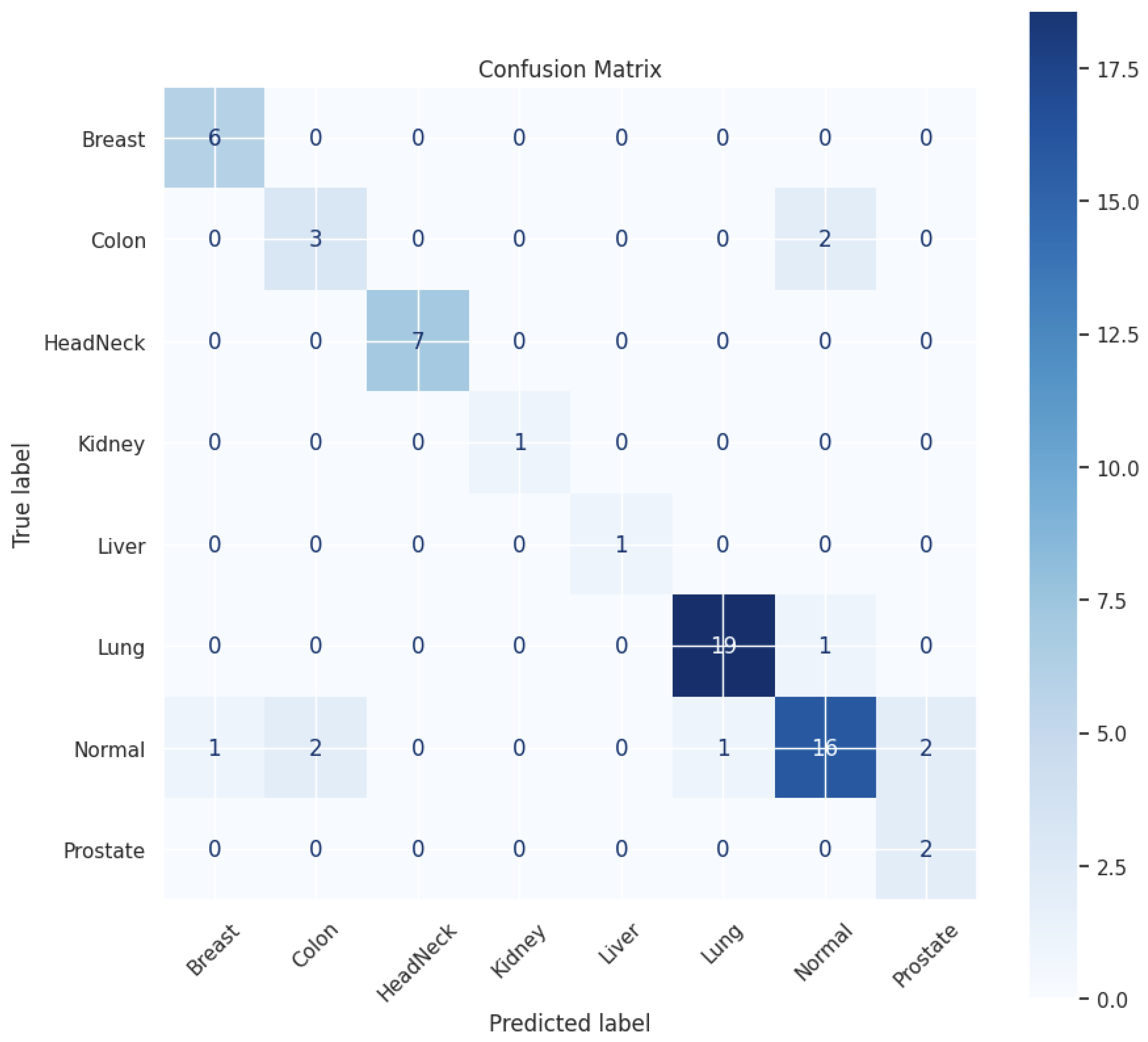
The confusion matrix for the eight classes is shown in Figure 16.
For the cancer type classification, the weighted average accuracy, precision, recall, F1 score, and G-Mean on validation data are, respectively, 91%, 87%, 86%, 86%, and 84%, achieved on eight classes. The distribution is given in Table 3.
We also compared the results of our methodology with the baseline study [95] shown in Figure 17. The results clearly show the improvements in the classification results and how our methodology outperformed the comparative study.
Our KEGG pathway enrichment analysis revealed a spectrum of cancer-associated genes, confirming our technology’s efficiency in discovering crucial cancer biomarkers [115]. Remarkably, genes associated with the “Transcriptional Misregulation in Cancer” [116,117] and “Acute Myeloid Leukemia” [118,119] pathways were enriched, showing the critical role of these genes in cancer development [120]. These pathways comprise well-established tumor suppressors like TP53 [121,122] and RB1 [123], frequently altered in different malignancies. Their identification confirms our technique, indicating that it can reliably reveal vital genetic causes of cancer [124]. Furthermore, genes related to “Choline Metabolism in Cancer” [125], a route gaining notoriety for its participation in cancer cell proliferation and metabolism, were also discovered [125]. These findings emphasize our model’s capabilities, not simply to uncover well-known pathways but also to highlight the expanding areas of cancer research, such as cancer metabolism.
The bar plot in Figure 18 shows the significant biological processes enriched in our dataset, which were identified by GO enrichment analysis. The processes shown, such as the ether lipid biosynthetic process [126], TRAIL-activated apoptotic signalling pathway [127], and glycerol ether metabolic process [128], are crucial in comprehending the underlying molecular mechanisms in cancer. Lipid biosynthesis and metabolism, which are strongly featured in this analysis, are known to play critical roles in cancer cell survival and proliferation, as cancer cells often reorganize their metabolic pathways to favor rapid growth [129,130]. Similarly, apoptotic mechanisms, such as the TRAIL-activated apoptotic signaling pathway, are crucial in regulating cell death, and their dysregulation is a hallmark of cancer [131]. The continuous relevance of these processes, as evidenced by the low adjusted p-values (p.adjust), ranges between 0.044 and 0.0045, demonstrating the robustness of our approach to identifying physiologically meaningful pathways. This underlines the efficacy of our technology in discovering possible biomarkers and uncovering essential cancer-related cellular processes. By employing XAI, our technique further provides insights into the crucial molecular mechanisms driving these classifications, thereby revealing potential novel therapeutic targets.
The XAI adds transparency and interpretability to the deep learning model’s predictions. Using LIME, we managed to examine the contribution of individual genes to the categorization decision. This allowed us to understand the role of specific genes in driving the enrichment of cancer-related pathways and how they contribute to the model’s decision-making process. For instance, genes found in “MicroRNAs in Cancer” and “Nicotinate and Nicotinamide Metabolism”, although not typically associated with well-established cancer pathways [132,133], were highlighted by XAI as significant contributors to classification. This indicates that these genes may have under-explored roles in cancer, making them possible new biomarkers for further research. The XAI framework thus not only increases our model’s prediction capacity but also helps validate the biological relevance of the genes identified, guaranteeing that the model’s output is biologically interpretable. By offering insights into how these genes influence classification outcomes, XAI offers a deeper understanding of our model’s predictions, helping to prioritize genes for experimental validation.

4. Conclusions

Deep learning advances have turned the technique into a valuable partner in the analysis of cancer causes, biomarkers, and prognosis in earlier stages of the disease.
In this paper, we applied deep learning, explainable AI, KEGG pathway enrichment analysis and data visualization to offer a robust, efficient and more reproducible pipeline to both classify different cancers with the same model and to trace relevant genes to the high performance of the models. In the process, we provided deep learning-based solutions to deal with data with highly imbalanced classes, large dimensions, and low instance numbers, all persistent issues when dealing with biological data.
Our approach utilizes a CNN architecture optimized for both binary and multiclass classification. The architecture, which incorporates numerous Conv1D layers, was designed to capture complex patterns in high-dimensional gene expression data, successfully discriminating between various cancer types with a single model.
Regularization techniques such as dropout and L2 regularization, paired with powerful optimizers like AdamW, guaranteed that the model remained robust and generalized well, even with a relatively limited dataset. Through KEGG pathway enrichment analysis, we effectively identified genes and pathways that are significantly related to cancer, including well-established genes involved in transcriptional misregulation and cancer metabolism. Additionally, our research identified lesser-known genes as relevant, suggesting their potential as novel cancer biomarkers.
The integration of XAI gave transparency into the model’s decision-making process, allowing us to understand which genes were central to the categorization outputs and thus biologically relevant. This use of XAI validated the model’s predictions but also created new paths for the discovery of previous biomarkers.
Overall, our study highlights the power of integrating deep learning with enrichment analysis and explainable AI to uncover both established and new biomarkers in cancer research. The methodology offers a scalable and interpretable framework for cancer classification and biomarker identification, paving the way for future applications in the development of personalized medicine and treatment. Furthermore, this architecture can be used to classify other kinds of cancer, and trained models can be used for transfer learning to learn better on the new dataset instead of learning from scratch. In the future, our goal is to improve our work by including larger and more diverse datasets, exploring the biological significance of novel genes and further refining the application of XAI in biomedical research.

Author Contributions

Conceptualization, H.Y. and R.M.; methodology, H.Y.; software, H.Y.; validation, H.Y. and R.M.; formal analysis, H.Y.; investigation, H.Y. and R.M.; resources, H.Y. and R.M.; data curation, H.Y.; writing—original draft preparation, H.Y.; writing—review and editing, R.M. and H.Y.; visualization, H.Y.; supervision, R.M.; project administration, R.M.; funding acquisition, R.M. All authors have read and agreed to the published version of the manuscript.

Funding

This publication emanated from research conducted with the financial support of Taighde Éireann—Research Ireland under grant number 18/CRT/6222. For the purpose of open access, the author applied a CC BY public copyright license to any Author Accepted Manuscript version arising from this submission.

Data Availability Statement

Data used in this research are available at https://sbcb.inf.ufrgs.br/research/barracurda (accessed on 15 May 2025).

Conflicts of Interest

The authors declare no conflicts of interest.

References

  1. World Health Organization. Cancer WHO Facts-Sheet. 2025. Available online: https://www.who.int/news-room/fact-sheets/detail/cancer (accessed on 1 July 2025).
  2. World Cancer Research Fund International. Worldwide Cancer Data | World Cancer Research Fund. 2025. Available online: https://www.wcrf.org/preventing-cancer/cancer-statistics/worldwide-cancer-data/ (accessed on 1 July 2025).
  3. Verma, G.; Luciani, M.L.; Palombo, A.; Metaxa, L.; Panzironi, G.; Pediconi, F.; Giuliani, A.; Bizzarri, M.; Todde, V. Microcalcification morphological descriptors and parenchyma fractal dimension hierarchically interact in breast cancer: A diagnostic perspective. Comput. Biol. Med. 2018, 93, 1–6. [Google Scholar] [CrossRef] [PubMed]
  4. Alizadeh, E.; Castle, J.; Quirk, A.; Taylor, C.D.; Xu, W.; Prasad, A. Cellular morphological features are predictive markers of cancer cell state. Comput. Biol. Med. 2020, 126, 104044. [Google Scholar] [CrossRef] [PubMed]
  5. Sakamoto, S.; Kikuchi, K. Expanding the cytological and architectural spectrum of mucoepidermoid carcinoma: The key to solving diagnostic problems in morphological variants. Semin. Diagn. Pathol. 2024, 41, 182–189. [Google Scholar] [CrossRef] [PubMed]
  6. Guerroudji, M.A.; Hadjadj, Z.; Lichouri, M.; Amara, K.; Zenati, N. Efficient machine learning-based approach for brain tumor detection using the CAD system. IETE J. Res. 2024, 70, 3664–3678. [Google Scholar] [CrossRef]
  7. Mallon, E.; Osin, P.; Nasiri, N.; Blain, I.; Howard, B.; Gusterson, B. The basic pathology of human breast cancer. J. Mammary Gland. Biol. Neoplasia 2000, 5, 139–163. [Google Scholar] [CrossRef]
  8. Allison, K.H. Molecular pathology of breast cancer: What a pathologist needs to know. Am. J. Clin. Pathol. 2012, 138, 770–780. [Google Scholar] [CrossRef]
  9. Kurman, R.J.; Shih, I.M. Pathogenesis of ovarian cancer: Lessons from morphology and molecular biology and their clinical implications. Int. J. Gynecol. Pathol. 2008, 27, 151–160. [Google Scholar] [CrossRef]
  10. Beck, A.H.; Sangoi, A.R.; Leung, S.; Marinelli, R.J.; Nielsen, T.O.; Van De Vijver, M.J.; West, R.B.; Van De Rijn, M.; Koller, D. Systematic analysis of breast cancer morphology uncovers stromal features associated with survival. Sci. Transl. Med. 2011, 3, 108ra113. [Google Scholar] [CrossRef]
  11. Meirovitz, A.; Nisman, B.; Allweis, T.M.; Carmon, E.; Kadouri, L.; Maly, B.; Maimon, O.; Peretz, T. Thyroid hormones and morphological features of primary breast cancer. Anticancer. Res. 2022, 42, 253–261. [Google Scholar] [CrossRef]
  12. do Nascimento, R.G.; Otoni, K.M. Histological and molecular classification of breast cancer: What do we know? Mastology 2020, 30, 1–8. [Google Scholar] [CrossRef]
  13. Gamble, P.; Jaroensri, R.; Wang, H.; Tan, F.; Moran, M.; Brown, T.; Flament-Auvigne, I.; Rakha, E.A.; Toss, M.; Dabbs, D.J.; et al. Determining breast cancer biomarker status and associated morphological features using deep learning. Commun. Med. 2021, 1, 14. [Google Scholar] [CrossRef] [PubMed]
  14. Oyelade, O.N.; Ezugwu, A.E. A novel wavelet decomposition and transformation convolutional neural network with data augmentation for breast cancer detection using digital mammogram. Sci. Rep. 2022, 12, 5913. [Google Scholar] [CrossRef] [PubMed]
  15. Mohammed, M.; Mwambi, H.; Mboya, I.B.; Elbashir, M.K.; Omolo, B. A stacking ensemble deep learning approach to cancer type classification based on TCGA data. Sci. Rep. 2021, 11, 15626. [Google Scholar] [CrossRef] [PubMed]
  16. Triantafyllou, A.; Dovrolis, N.; Zografos, E.; Theodoropoulos, C.; Zografos, G.C.; Michalopoulos, N.V.; Gazouli, M. Circulating miRNA expression profiling in breast cancer molecular subtypes: Applying machine learning analysis in bioinformatics. Cancer Diagn. Progn. 2022, 2, 739. [Google Scholar] [CrossRef]
  17. Almarzouki, H.Z. Deep-learning-based cancer profiles classification using gene expression data profile. J. Healthc. Eng. 2022, 2022, 4715998. [Google Scholar] [CrossRef]
  18. Aziz, R.M. Nature-inspired metaheuristics model for gene selection and classification of biomedical microarray data. Med. Biol. Eng. Comput. 2022, 60, 1627–1646. [Google Scholar] [CrossRef]
  19. Ogundokun, R.O.; Misra, S.; Douglas, M.; Damaševičius, R.; Maskeliūnas, R. Medical internet-of-things based breast cancer diagnosis using hyperparameter-optimized neural networks. Future Internet 2022, 14, 153. [Google Scholar] [CrossRef]
  20. Chowdhary, C.L.; Khare, N.; Patel, H.; Koppu, S.; Kaluri, R.; Rajput, D.S. Past, present and future of gene feature selection for breast cancer classification—A survey. Int. J. Eng. Syst. Model. Simul. 2022, 13, 140–153. [Google Scholar] [CrossRef]
  21. Amethiya, Y.; Pipariya, P.; Patel, S.; Shah, M. Comparative analysis of breast cancer detection using machine learning and biosensors. Intell. Med. 2022, 2, 69–81. [Google Scholar] [CrossRef]
  22. Geraci, F.; Saha, I.; Bianchini, M. RNA-Seq analysis: Methods, applications and challenges. Front. Genet. 2020, 11, 220. [Google Scholar] [CrossRef]
  23. Hrdlickova, R.; Toloue, M.; Tian, B. RNA-Seq methods for transcriptome analysis. Wiley Interdiscip. Rev. RNA 2017, 8, e1364. [Google Scholar] [CrossRef]
  24. Van den Berge, K.; Hembach, K.M.; Soneson, C.; Tiberi, S.; Clement, L.; Love, M.I.; Patro, R.; Robinson, M.D. RNA sequencing data: Hitchhiker’s guide to expression analysis. Annu. Rev. Biomed. Data Sci. 2019, 2, 139–173. [Google Scholar] [CrossRef]
  25. Lam, H.Y.; Clark, M.J.; Chen, R.; Chen, R.; Natsoulis, G.; O’huallachain, M.; Dewey, F.E.; Habegger, L.; Ashley, E.A.; Gerstein, M.B.; et al. Performance comparison of whole-genome sequencing platforms. Nat. Biotechnol. 2012, 30, 78–82. [Google Scholar] [CrossRef] [PubMed]
  26. Jeon, S.A.; Park, J.L.; Park, S.J.; Kim, J.H.; Goh, S.H.; Han, J.Y.; Kim, S.Y. Comparison between MGI and Illumina sequencing platforms for whole genome sequencing. Genes Genom. 2021, 43, 713–724. [Google Scholar] [CrossRef] [PubMed]
  27. Fouhy, F.; Clooney, A.G.; Stanton, C.; Claesson, M.J.; Cotter, P.D. 16S rRNA gene sequencing of mock microbial populations-impact of DNA extraction method, primer choice and sequencing platform. BMC Microbiol. 2016, 16, 1–13. [Google Scholar] [CrossRef]
  28. Hu, T.; Chitnis, N.; Monos, D.; Dinh, A. Next-generation sequencing technologies: An overview. Hum. Immunol. 2021, 82, 801–811. [Google Scholar] [CrossRef]
  29. Gandhi, V.V.; Samuels, D.C. A review comparing deoxyribonucleoside triphosphate (dNTP) concentrations in the mitochondrial and cytoplasmic compartments of normal and transformed cells. Nucleosides Nucleotides Nucleic Acids 2011, 30, 317–339. [Google Scholar] [CrossRef]
  30. Rai, M.F.; Tycksen, E.D.; Sandell, L.J.; Brophy, R.H. Advantages of RNA-seq compared to RNA microarrays for transcriptome profiling of anterior cruciate ligament tears. J. Orthop. Res. 2018, 36, 484–497. [Google Scholar] [CrossRef]
  31. Li, W.V.; Li, J.J. Modeling and analysis of RNA-seq data: A review from a statistical perspective. Quant. Biol. 2018, 6, 195–209. [Google Scholar] [CrossRef]
  32. National Academies of Sciences, Engineering, and Medicine and Mapping of RNA Modifications Committee. Driving Innovation to Study RNA Modifications. In Charting a Future for Sequencing RNA and Its Modifications: A New Era for Biology and Medicine; National Academies Press (US): Washington, DC, USA, 2024. [Google Scholar]
  33. Zhao, S.; Fung-Leung, W.P.; Bittner, A.; Ngo, K.; Liu, X. Comparison of RNA-Seq and microarray in transcriptome profiling of activated T cells. PLoS ONE 2014, 9, e78644. [Google Scholar] [CrossRef]
  34. Zararsız, G. Development and application of novel machine learning approaches for RNA-seq data classification. Int. J. Comput. Trends Tech. 2015, 2017, 62–64. [Google Scholar]
  35. Gondane, A.; Itkonen, H.M. Revealing the history and mystery of RNA-Seq. Curr. Issues Mol. Biol. 2023, 45, 1860–1874. [Google Scholar] [CrossRef] [PubMed]
  36. Epstein, C.B.; Butow, R.A. Microarray technology—Enhanced versatility, persistent challenge. Curr. Opin. Biotechnol. 2000, 11, 36–41. [Google Scholar] [CrossRef] [PubMed]
  37. Blohm, D.H.; Guiseppi-Elie, A. New developments in microarray technology. Curr. Opin. Biotechnol. 2001, 12, 41–47. [Google Scholar] [CrossRef]
  38. Blalock, E.M. A Beginner’s Guide to Microarrays; Springer Science & Business Media: Berlin/Heidelberg, Germany, 2003. [Google Scholar]
  39. Feltes, B.C.; Chandelier, E.B.; Grisci, B.I.; Dorn, M. Cumida: An extensively curated microarray database for benchmarking and testing of machine learning approaches in cancer research. J. Comput. Biol. 2019, 26, 376–386. [Google Scholar] [CrossRef]
  40. Verleysen, M.; François, D. The curse of dimensionality in data mining and time series prediction. In Proceedings of the International Work-Conference on Artificial Neural Networks, Barcelona, Spain, 8–10 June 2005; Springer: Berlin/Heidelberg, Germany, 2005; pp. 758–770. [Google Scholar]
  41. Khalsan, M.; Machado, L.R.; Al-Shamery, E.S.; Ajit, S.; Anthony, K.; Mu, M.; Agyeman, M.O. A survey of machine learning approaches applied to gene expression analysis for cancer prediction. IEEE Access 2022, 10, 27522–27534. [Google Scholar] [CrossRef]
  42. Yuan, F.; Lu, L.; Zou, Q. Analysis of gene expression profiles of lung cancer subtypes with machine learning algorithms. Biochim. Biophys. Acta (BBA) Mol. Basis Dis. 2020, 1866, 165822. [Google Scholar] [CrossRef]
  43. Wang, D.; Li, J.R.; Zhang, Y.H.; Chen, L.; Huang, T.; Cai, Y.D. Identification of differentially expressed genes between original breast cancer and xenograft using machine learning algorithms. Genes 2018, 9, 155. [Google Scholar] [CrossRef]
  44. Pisner, D.A.; Schnyer, D.M. Support vector machine. In Machine Learning; Elsevier: Amsterdam, The Netherlands, 2020; pp. 101–121. [Google Scholar]
  45. Meddouri, N.; Khoufi, H.; Maddouri, M. DFC: A Performant Dagging Approach of Classification Based on Formal Concept. Int. J. Artif. Intell. Mach. Learn. (IJAIML) 2021, 11, 38–62. [Google Scholar] [CrossRef]
  46. Liu, Y.; Wang, Y.; Zhang, J. New machine learning algorithm: Random forest. In Proceedings of the Information Computing and Applications: Third International Conference, ICICA 2012, Chengde, China, 14–16 September 2012; Springer: Berlin/Heidelberg, Germany, 2012; pp. 246–252. [Google Scholar]
  47. Dramiński, M.; Rada-Iglesias, A.; Enroth, S.; Wadelius, C.; Koronacki, J.; Komorowski, J. Monte Carlo feature selection for supervised classification. Bioinformatics 2008, 24, 110–117. [Google Scholar] [CrossRef]
  48. Danaee, P.; Ghaeini, R.; Hendrix, D.A. A deep learning approach for cancer detection and relevant gene identification. In Proceedings of the Pacific Symposium on Biocomputing 2017, Waimea, HI, USA, 3–7 January 2017; World Scientific: Singapore, 2017; pp. 219–229. [Google Scholar]
  49. Jia, D.; Chen, C.; Chen, C.; Chen, F.; Zhang, N.; Yan, Z.; Lv, X. Breast cancer case identification based on deep learning and bioinformatics analysis. Front. Genet. 2021, 12, 628136. [Google Scholar] [CrossRef]
  50. Clough, E.; Barrett, T. The gene expression omnibus database. In Statistical Genomics: Methods and Protocols; Springer: New York, NY, USA, 2016; pp. 93–110. [Google Scholar]
  51. Deng, M.; Brägelmann, J.; Schultze, J.L.; Perner, S. Web-TCGA: An online platform for integrated analysis of molecular cancer data sets. BMC Bioinform. 2016, 17, 72. [Google Scholar] [CrossRef]
  52. Alshareef, A.M.; Alsini, R.; Alsieni, M.; Alrowais, F.; Marzouk, R.; Abunadi, I.; Nemri, N. Optimal deep learning enabled prostate cancer detection using microarray gene expression. J. Healthc. Eng. 2022, 2022, 7364704. [Google Scholar] [CrossRef] [PubMed]
  53. Ma, Q.; Xu, D. Deep learning shapes single-cell data analysis. Nat. Rev. Mol. Cell Biol. 2022, 23, 303–304. [Google Scholar] [CrossRef] [PubMed]
  54. Kaveh, M.; Mesgari, M.S. Application of meta-heuristic algorithms for training neural networks and deep learning architectures: A comprehensive review. Neural Process. Lett. 2023, 55, 4519–4622. [Google Scholar] [CrossRef] [PubMed]
  55. Zhang, W.; Gu, X.; Tang, L.; Yin, Y.; Liu, D.; Zhang, Y. Application of machine learning, deep learning and optimization algorithms in geoengineering and geoscience: Comprehensive review and future challenge. Gondwana Res. 2022, 109, 1–17. [Google Scholar] [CrossRef]
  56. Abdel-Basset, M.; Abdel-Fatah, L.; Sangaiah, A.K. Metaheuristic algorithms: A comprehensive review. In Computational Intelligence for Multimedia Big Data on the Cloud with Engineering Applications; Elsevier: Amsterdam, The Netherlands, 2018; pp. 185–231. [Google Scholar]
  57. Rahman, M.A.; Sokkalingam, R.; Othman, M.; Biswas, K.; Abdullah, L.; Abdul Kadir, E. Nature-inspired metaheuristic techniques for combinatorial optimization problems: Overview and recent advances. Mathematics 2021, 9, 2633. [Google Scholar] [CrossRef]
  58. Tkatek, S.; Bahti, O.; Lmzouari, Y.; Abouchabaka, J. Artificial intelligence for improving the optimization of NP-hard problems: A review. Int. J. Adv. Trends Comput. Sci. Appl. 2020, 9, 7411–7420. [Google Scholar]
  59. Mandal, A.K.; Dehuri, S. A survey on ant colony optimization for solving some of the selected np-hard problem. In Proceedings of the Biologically Inspired Techniques in Many-Criteria Decision Making: International Conference on Biologically Inspired Techniques in Many-Criteria Decision Making (BITMDM-2019), Balasore, India, 19–20 December 2019; Springer: Berlin/Heidelberg, Germany, 2020; pp. 85–100. [Google Scholar]
  60. Calvet, L.; Benito, S.; Juan, A.A.; Prados, F. On the role of metaheuristic optimization in bioinformatics. Int. Trans. Oper. Res. 2023, 30, 2909–2944. [Google Scholar] [CrossRef]
  61. Shukla, A.K.; Tripathi, D.; Reddy, B.R.; Chandramohan, D. A study on metaheuristics approaches for gene selection in microarray data: Algorithms, applications and open challenges. Evol. Intell. 2020, 13, 309–329. [Google Scholar] [CrossRef]
  62. Chakraborty, S.; Mali, K.; Chatterjee, S.; Banerjee, S.; Mazumdar, K.G.; Debnath, M.; Basu, P.; Bose, S.; Roy, K. Detection of skin disease using metaheuristic supported artificial neural networks. In Proceedings of the 2017 8th Annual Industrial Automation and Electromechanical Engineering Conference (IEMECON), Bangkok, Thailand, 16–18 August 2017; pp. 224–229. [Google Scholar] [CrossRef]
  63. MotieGhader, H.; Masoudi-Sobhanzadeh, Y.; Ashtiani, S.H.; Masoudi-Nejad, A. mRNA and microRNA selection for breast cancer molecular subtype stratification using meta-heuristic based algorithms. Genomics 2020, 112, 3207–3217. [Google Scholar] [CrossRef] [PubMed]
  64. Onwubolu, G.C.; Mutingi, M. A genetic algorithm approach to cellular manufacturing systems. Comput. Ind. Eng. 2001, 39, 125–144. [Google Scholar] [CrossRef]
  65. Masoudi-Sobhanzadeh, Y.; Motieghader, H. World Competitive Contests (WCC) algorithm: A novel intelligent optimization algorithm for biological and non-biological problems. Inform. Med. Unlocked 2016, 3, 15–28. [Google Scholar] [CrossRef]
  66. Zhu, H.; Wang, Y.; Wang, K.; Chen, Y. Particle Swarm Optimization (PSO) for the constrained portfolio optimization problem. Expert Syst. Appl. 2011, 38, 10161–10169. [Google Scholar] [CrossRef]
  67. Gandomi, A.H.; Yang, X.S.; Alavi, A.H. Cuckoo search algorithm: A metaheuristic approach to solve structural optimization problems. Eng. Comput. 2013, 29, 17–35. [Google Scholar] [CrossRef]
  68. Kaveh, A.; Kaveh, A. Imperialist competitive algorithm. In Advances in Metaheuristic Algorithms for Optimal Design of Structures; Springer: Berlin/Heidelberg, Germany, 2017; pp. 353–373. [Google Scholar]
  69. Li, W.; Özcan, E.; John, R. A learning automata-based multiobjective hyper-heuristic. IEEE Trans. Evol. Comput. 2017, 23, 59–73. [Google Scholar] [CrossRef]
  70. Patel, V.K.; Savsani, V.J. Heat transfer search (HTS): A novel optimization algorithm. Inf. Sci. 2015, 324, 217–246. [Google Scholar] [CrossRef]
  71. Dorigo, M.; Birattari, M.; Stutzle, T. Ant colony optimization. IEEE Comput. Intell. Mag. 2006, 1, 28–39. [Google Scholar] [CrossRef]
  72. Ghaemi, M.; Feizi-Derakhshi, M.R. Forest optimization algorithm. Expert Syst. Appl. 2014, 41, 6676–6687. [Google Scholar] [CrossRef]
  73. Ezugwu, A.E.; Prayogo, D. Symbiotic organisms search algorithm: Theory, recent advances and applications. Expert Syst. Appl. 2019, 119, 184–209. [Google Scholar] [CrossRef]
  74. Kashan, A.H. League Championship Algorithm (LCA): An algorithm for global optimization inspired by sport championships. Appl. Soft Comput. 2014, 16, 171–200. [Google Scholar] [CrossRef]
  75. Wei, K.; Li, T.; Huang, F.; Chen, J.; He, Z. Cancer classification with data augmentation based on generative adversarial networks. Front. Comput. Sci. 2022, 16, 162601. [Google Scholar] [CrossRef]
  76. Deng, X.; Li, M.; Deng, S.; Wang, L. Hybrid gene selection approach using XGBoost and multi-objective genetic algorithm for cancer classification. Med. Biol. Eng. Comput. 2022, 60, 663–681. [Google Scholar] [CrossRef] [PubMed]
  77. Younis, H.; Bhatti, M.H.; Azeem, M. Classification of Skin Cancer Dermoscopy Images using Transfer Learning. In Proceedings of the 2019 15th International Conference on Emerging Technologies (ICET), Peshawar, Pakistan, 2–3 December 2019; pp. 1–4. [Google Scholar] [CrossRef]
  78. Xie, X.; Wang, X.; Liang, Y.; Yang, J.; Wu, Y.; Li, L.; Sun, X.; Bing, P.; He, B.; Tian, G.; et al. Evaluating cancer-related biomarkers based on pathological images: A systematic review. Front. Oncol. 2021, 11, 763527. [Google Scholar] [CrossRef]
  79. Yadav, S.S.; Jadhav, S.M. Thermal infrared imaging based breast cancer diagnosis using machine learning techniques. Multimed. Tools Appl. 2022, 81, 13139–13157. [Google Scholar] [CrossRef]
  80. Aljuaid, H.; Alturki, N.; Alsubaie, N.; Cavallaro, L.; Liotta, A. Computer-aided diagnosis for breast cancer classification using deep neural networks and transfer learning. Comput. Methods Programs Biomed. 2022, 223, 106951. [Google Scholar] [CrossRef]
  81. Karamti, H.; Alharthi, R.; Umer, M.; Shaiba, H.; Ishaq, A.; Abuzinadah, N.; Alsubai, S.; Ashraf, I. Breast cancer detection employing stacked ensemble model with convolutional features. Cancer Biomarkers 2023, 40, 155–170. [Google Scholar] [CrossRef]
  82. Munshi, R.M.; Cascone, L.; Alturki, N.; Saidani, O.; Alshardan, A.; Umer, M. A novel approach for breast cancer detection using optimized ensemble learning framework and XAI. Image Vis. Comput. 2024, 142, 104910. [Google Scholar] [CrossRef]
  83. Wani, N.A.; Kumar, R.; Bedi, J. DeepXplainer: An interpretable deep learning based approach for lung cancer detection using explainable artificial intelligence. Comput. Methods Programs Biomed. 2024, 243, 107879. [Google Scholar] [CrossRef]
  84. Dwivedi, R.; Dave, D.; Naik, H.; Singhal, S.; Omer, R.; Patel, P.; Qian, B.; Wen, Z.; Shah, T.; Morgan, G.; et al. Explainable AI (XAI): Core ideas, techniques, and solutions. ACM Comput. Surv. 2023, 55, 1–33. [Google Scholar] [CrossRef]
  85. Salih, A.M.; Raisi-Estabragh, Z.; Galazzo, I.B.; Radeva, P.; Petersen, S.E.; Lekadir, K.; Menegaz, G. A Perspective on Explainable Artificial Intelligence Methods: SHAP and LIME. Adv. Intell. Syst. 2024, 7, 2400304. [Google Scholar] [CrossRef]
  86. Sulaiman, M.H.; Mustaffa, Z.; Saari, M.M.; Daniyal, H.; Musirin, I.; Daud, M.R. Barnacles mating optimizer: An evolutionary algorithm for solving optimization. In Proceedings of the 2018 IEEE International Conference on Automatic Control and Intelligent Systems (I2CACIS), Shah Alam, Malaysia, 20 October 2018; pp. 99–104. [Google Scholar]
  87. Houssein, E.H.; Abdelminaam, D.S.; Hassan, H.N.; Al-Sayed, M.M.; Nabil, E. A hybrid barnacles mating optimizer algorithm with support vector machines for gene selection of microarray cancer classification. IEEE Access 2021, 9, 64895–64905. [Google Scholar] [CrossRef]
  88. Karaboga, D. Artificial bee colony algorithm. scholarpedia 2010, 5, 6915. [Google Scholar] [CrossRef]
  89. Kaur, S.; Awasthi, L.K.; Sangal, A.L.; Dhiman, G. Tunicate Swarm Algorithm: A new bio-inspired based metaheuristic paradigm for global optimization. Eng. Appl. Artif. Intell. 2020, 90, 103541. [Google Scholar] [CrossRef]
  90. Chakraborty, S.; Sharma, S.; Saha, A.K.; Saha, A. A novel improved whale optimization algorithm to solve numerical optimization and real-world applications. Artif. Intell. Rev. 2022, 55, 4605–4716. [Google Scholar] [CrossRef]
  91. Devi, S.S.; Prithiviraj, K. Breast cancer classification with microarray gene expression data based on improved whale optimization algorithm. Int. J. Swarm Intell. Res. (IJSIR) 2023, 14, 1–21. [Google Scholar] [CrossRef]
  92. Mohamed, T.I.; Ezugwu, A.E.; Fonou-Dombeu, J.V.; Ikotun, A.M.; Mohammed, M. A bio-inspired convolution neural network architecture for automatic breast cancer detection and classification using RNA-Seq gene expression data. Sci. Rep. 2023, 13, 14644. [Google Scholar] [CrossRef]
  93. JagadeeswaraRao, G.; Sivaprasad, A. An integrated ensemble learning technique for gene expression classification and biomarker identification from RNA-seq data for pancreatic cancer prognosis. Int. J. Inf. Technol. 2024, 16, 1505–1516. [Google Scholar] [CrossRef]
  94. Wang, J.; Huang, J.; Hu, Y.; Guo, Q.; Zhang, S.; Tian, J.; Niu, Y.; Ji, L.; Xu, Y.; Tang, P.; et al. Terminal modifications independent cell-free RNA sequencing enables sensitive early cancer detection and classification. Nat. Commun. 2024, 15, 156. [Google Scholar] [CrossRef]
  95. Feltes, B.C.; Poloni, J.D.F.; Dorn, M. Benchmarking and testing machine learning approaches with BARRA: CuRDa, a curated RNA-seq database for cancer research. J. Comput. Biol. 2021, 28, 931–944. [Google Scholar] [CrossRef]
  96. Quinlan, J.R. Learning decision tree classifiers. ACM Computing Surveys (CSUR) 1996, 28, 71–72. [Google Scholar] [CrossRef]
  97. Larose, D.T.; Larose, C.D. k-nearest neighbor algorithm. In Discovering Knowledge in Data: An Introduction to Data Mining; IEEE: New York, NY, USA, 2014. [Google Scholar]
  98. Taud, H.; Mas, J.F. Multilayer perceptron (MLP). Geomatic Approaches for Modeling Land Change Scenarios; Springer: Cham, Switzerland, 2018; pp. 451–455. [Google Scholar]
  99. Elbashir, M.K.; Ezz, M.; Mohammed, M.; Saloum, S.S. Lightweight convolutional neural network for breast cancer classification using RNA-seq gene expression data. IEEE Access 2019, 7, 185338–185348. [Google Scholar] [CrossRef]
  100. Alharbi, F.; Vakanski, A.; Zhang, B.; Elbashir, M.K.; Mohammed, M. Comparative Analysis of Multi-Omics Integration Using Graph Neural Networks for Cancer Classification. IEEE Access 2025, 13, 37724–37736. [Google Scholar] [CrossRef]
  101. Davis, S.; Meltzer, P.S. GEOquery: A bridge between the Gene Expression Omnibus (GEO) and BioConductor. Bioinformatics 2007, 23, 1846–1847. [Google Scholar] [CrossRef]
  102. Wingett, S.W.; Andrews, S. FastQ Screen: A tool for multi-genome mapping and quality control. F1000Research 2018, 7, 1338. [Google Scholar] [CrossRef]
  103. Bolger, A.M.; Lohse, M.; Usadel, B. Trimmomatic: A flexible trimmer for Illumina sequence data. Bioinformatics 2014, 30, 2114–2120. [Google Scholar] [CrossRef]
  104. Dobin, A.; Davis, C.A.; Schlesinger, F.; Drenkow, J.; Zaleski, C.; Jha, S.; Batut, P.; Chaisson, M.; Gingeras, T.R. STAR: Ultrafast universal RNA-seq aligner. Bioinformatics 2013, 29, 15–21. [Google Scholar] [CrossRef]
  105. Li, B.; Dewey, C.N. RSEM: Accurate transcript quantification from RNA-Seq data with or without a reference genome. BMC Bioinform. 2011, 12, 323. [Google Scholar] [CrossRef] [PubMed]
  106. Love, M.I.; Huber, W.; Anders, S. Moderated estimation of fold change and dispersion for RNA-seq data with DESeq2. Genome Biol. 2014, 15, 550. [Google Scholar] [CrossRef] [PubMed]
  107. Soneson, C.; Love, M.I.; Robinson, M.D. Differential analyses for RNA-seq: Transcript-level estimates improve gene-level inferences. F1000Research 2015, 4, 1521. [Google Scholar] [CrossRef] [PubMed]
  108. Chawla, N.V.; Bowyer, K.W.; Hall, L.O.; Kegelmeyer, W.P. SMOTE: Synthetic minority over-sampling technique. J. Artif. Intell. Res. 2002, 16, 321–357. [Google Scholar] [CrossRef]
  109. Maćkiewicz, A.; Ratajczak, W. Principal components analysis (PCA). Comput. Geosci. 1993, 19, 303–342. [Google Scholar] [CrossRef]
  110. Ige, A.O.; Sibiya, M. State-of-the-art in 1D Convolutional Neural Networks: A survey. IEEE Access 2024, 12, 144082–144105. [Google Scholar] [CrossRef]
  111. Roeder, L. Netron: Visualizer for Neural Network, Deep Learning and Machine Learning Models. 2025. Available online: https://github.com/lutzroeder/netron (accessed on 22 July 2025).
  112. Gygi, J.P.; Kleinstein, S.H.; Guan, L. Predictive overfitting in immunological applications: Pitfalls and solutions. Hum. Vaccines Immunother. 2023, 19, 2251830. [Google Scholar] [CrossRef] [PubMed]
  113. Yu, G.; Wang, L.G.; Han, Y.; He, Q.Y. clusterProfiler: An R package for comparing biological themes among gene clusters. Omics J. Integr. Biol. 2012, 16, 284–287. [Google Scholar] [CrossRef] [PubMed]
  114. Ostell, J.M. Entrez: The NCBI search and discovery engine. In Proceedings of the Data Integration in the Life Sciences: 8th International Conference, DILS 2012, College Park, MD, USA, 28–29 June 2012; Springer: Berlin/Heidelberg, Germany, 2012; pp. 1–4. [Google Scholar]
  115. Chen, L.; Zhang, Y.H.; Lu, G.; Huang, T.; Cai, Y.D. Analysis of cancer-related lncRNAs using gene ontology and KEGG pathways. Artif. Intell. Med. 2017, 76, 27–36. [Google Scholar] [CrossRef]
  116. Yuan, Y.; Cao, W.; Zhou, H.; Qian, H.; Wang, H. H2A. Z acetylation by lincZNF337-AS1 via KAT5 implicated in the transcriptional misregulation in cancer signaling pathway in hepatocellular carcinoma. Cell Death Dis. 2021, 12, 609. [Google Scholar] [CrossRef]
  117. Casamassimi, A.; Ciccodicola, A.; Rienzo, M. Transcriptional regulation and its misregulation in human diseases. Int. J. Mol. Sci. 2023, 24, 8640. [Google Scholar] [CrossRef]
  118. Lowenberg, B.; Downing, J.R.; Burnett, A. Acute myeloid leukemia. N. Engl. J. Med. 1999, 341, 1051–1062. [Google Scholar] [CrossRef]
  119. DiNardo, C.D.; Erba, H.P.; Freeman, S.D.; Wei, A.H. Acute myeloid leukaemia. Lancet 2023, 401, 2073–2086. [Google Scholar] [CrossRef]
  120. Kayser, S.; Levis, M.J. The clinical impact of the molecular landscape of acute myeloid leukemia. Haematologica 2023, 108, 308. [Google Scholar] [CrossRef]
  121. Sánchez-Heras, A.B.; Ramon y Cajal, T.; Pineda, M.; Aguirre, E.; Graña, B.; Chirivella, I.; Balmaña, J.; Brunet, J.; SEOM Hereditary Cancer Working Group; AEGH Hereditary Cancer Committee. SEOM clinical guideline on heritable TP53-related cancer syndrome (2022). Clin. Transl. Oncol. 2023, 25, 2627–2633. [Google Scholar] [CrossRef]
  122. Mansur, M.B.; Greaves, M. Convergent TP53 loss and evolvability in cancer. BMC Ecol. Evol. 2023, 23, 54. [Google Scholar] [CrossRef]
  123. Yuzhalin, A.E.; Lowery, F.J.; Saito, Y.; Yuan, X.; Yao, J.; Duan, Y.; Ding, J.; Acharya, S.; Zhang, C.; Fajardo, A.; et al. Astrocyte-induced Cdk5 expedites breast cancer brain metastasis by suppressing MHC-I expression to evade immune recognition. Nat. Cell Biol. 2024, 26, 1773–1789. [Google Scholar] [CrossRef]
  124. Jäger, D.; Berger, A.; Tuch, A.; Luckner-Minden, C.; Eurich, R.; Hlevnjak, M.; Schneeweiss, A.; Lichter, P.; Aulmann, S.; Heussel, C.P.; et al. Novel chimeric antigen receptors for the effective and safe treatment of NY-BR-1 positive breast cancer. Clin. Transl. Med. 2024, 14, e1776. [Google Scholar] [CrossRef]
  125. Li, X.; Hu, Z.; Shi, Q.; Qiu, W.; Liu, Y.; Liu, Y.; Huang, S.; Liang, L.; Chen, Z.; He, X. Elevated choline drives KLF5-dominated transcriptional reprogramming to facilitate liver cancer progression. Oncogene 2024, 43, 3121–3136. [Google Scholar] [CrossRef] [PubMed]
  126. Papin, M.; Bouchet, A.M.; Chantôme, A.; Vandier, C. Ether-lipids and cellular signaling: A differential role of alkyl-and alkenyl-ether-lipids? Biochimie 2023, 215, 50–59. [Google Scholar] [CrossRef] [PubMed]
  127. Geismann, C.; Hauser, C.; Grohmann, F.; Schneeweis, C.; Bölter, N.; Gundlach, J.P.; Schneider, G.; Röcken, C.; Meinhardt, C.; Schäfer, H.; et al. NF-κB/RelA controlled A20 limits TRAIL-induced apoptosis in pancreatic cancer. Cell Death Dis. 2023, 14, 3. [Google Scholar] [CrossRef] [PubMed]
  128. Solanki, R.; Bhatia, D. Stimulus-responsive hydrogels for targeted cancer therapy. Gels 2024, 10, 440. [Google Scholar] [CrossRef]
  129. Han, H.; Santos, H.A. Nano-and Micro-Platforms in Therapeutic Proteins Delivery for Cancer Therapy: Materials and Strategies. Adv. Mater. 2024, 36, 2409522. [Google Scholar] [CrossRef]
  130. Feng, T.Y.; Melchor, S.J.; Zhao, X.Y.; Ghumman, H.; Kester, M.; Fox, T.E.; Ewald, S.E. Tricarboxylic acid (TCA) cycle, sphingolipid, and phosphatidylcholine metabolism are dysregulated in T. gondii infection-induced cachexia. Heliyon 2023, 9, e17411. [Google Scholar] [CrossRef]
  131. Guerrache, A.; Micheau, O. TNF-Related Apoptosis-Inducing Ligand: Non-Apoptotic Signalling. Cells 2024, 13, 521. [Google Scholar] [CrossRef]
  132. Benjamin, C.; Crews, R. Nicotinamide Mononucleotide Supplementation: Understanding Metabolic Variability and Clinical Implications. Metabolites 2024, 14, 341. [Google Scholar] [CrossRef]
  133. Migaud, M.E.; Ziegler, M.; Baur, J.A. Regulation of and challenges in targeting NAD+ metabolism. Nat. Rev. Mol. Cell Biol. 2024, 25, 822–840. [Google Scholar] [CrossRef]
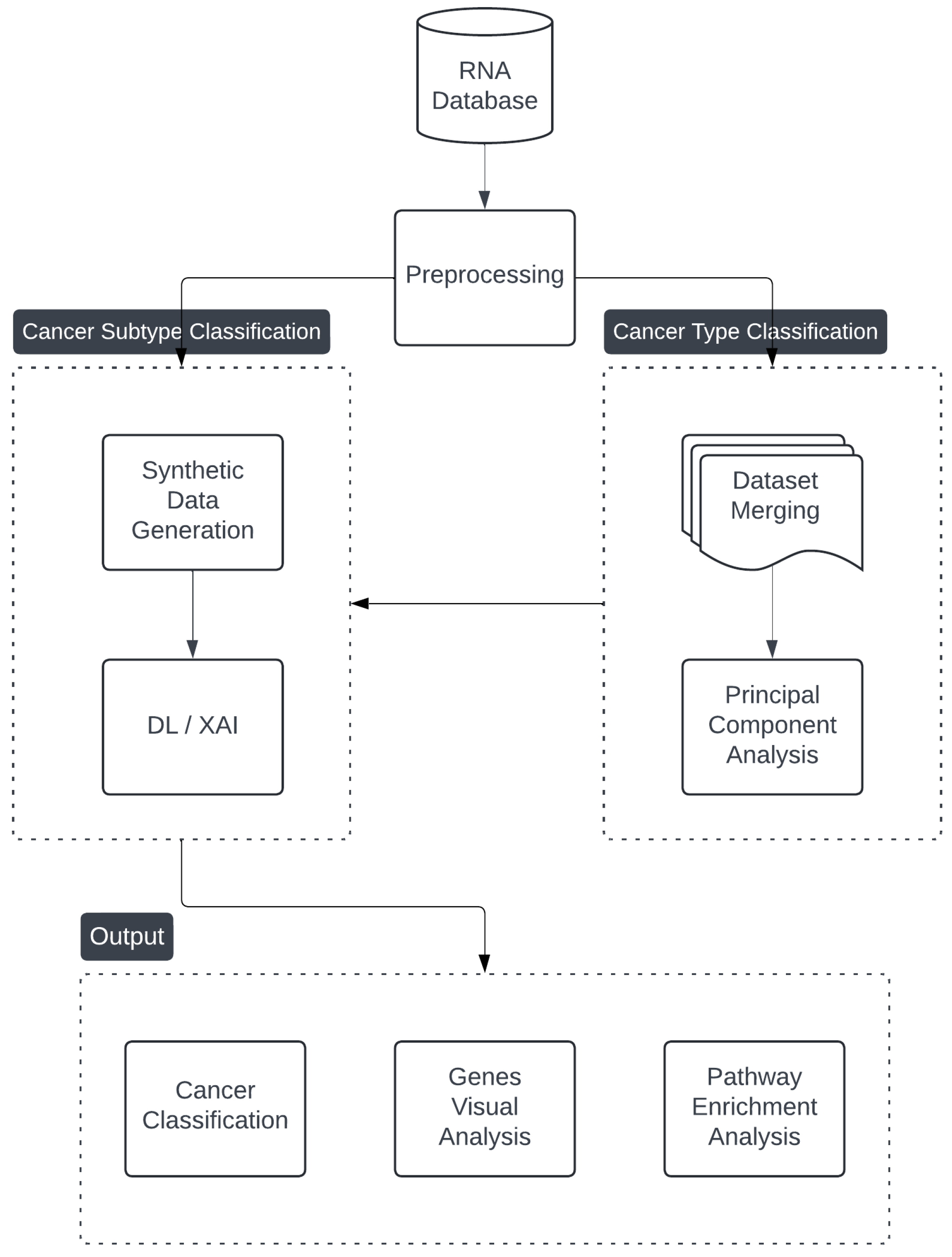
Figure 1. Overview of our methodology.
Make 07 00114 g001
Figure 2. Model architecture for cancer subtype classification (figure generated using Netron [111]).
Make 07 00114 g002
Figure 3. Model architecture for cancer type classification (figure generated using Netron [111]).
Make 07 00114 g003
Figure 4. Data point distribution of tumor (purple) and normal (red) profiles.
Make 07 00114 g004
Figure 5. Results of cancer classification model for binary class.
Make 07 00114 g005
Figure 6. Abundance value distribution of top genes for tissue GSE87340.
Make 07 00114 g006
Figure 7. Cluster map of top genes for tissue GSE87340. Columns correspond to genes, and rows correspond to samples. The color bar indicates normalized expression values.
Make 07 00114 g007
Figure 8. Results of cancer classification model for multi-class tasks.
Make 07 00114 g008
Figure 9. Data point distribution of Primary tumor (orange), Normal (green), Normal Liver (purple), Metastasis (blue).
Make 07 00114 g009
Figure 10. Abundance value distribution of top genes for tissue SRR2089755.
Make 07 00114 g010
Figure 11. Cluster map of top genes for tissue SRR2089755. Columns correspond to genes, and rows correspond to samples. The color bar indicates normalised expression values.
Make 07 00114 g011
Figure 12. Results of cancer type classification model (8 classes).
Make 07 00114 g012
Figure 13. Data point distribution of cancer types and Normal.
Make 07 00114 g013
Figure 14. Cluster map of top genes for 8 classes. Columns correspond to genes, and rows correspond to samples. The color bar indicates normalized expression values.
Make 07 00114 g014
Figure 15. Abundance value distribution of top genes for 8 classes.
Make 07 00114 g015
Figure 16. Confusion matrix for cancer type classification.
Make 07 00114 g016
Figure 17. Comparison between proposed method and base method.
Make 07 00114 g017
Figure 18. Gene ontology (GO) enrichment analysis.
Make 07 00114 g018
Table 1. Comparative Analysis of Relevant Studies.
YearStudyMethodResultOptimizedDSASDMCTSA
2017Danaee et al. [48]SDAE98.29% Acc
2018Wang et al. [43]PDXMCC (0.777) 92.9% Acc
2019Elbashir et al. [99]CNN98.76% Acc
2020Yuan et al. [42]SVM, RF100% Acc
2020MotieGhader et al. [63]Metaheuristic with SVM90% Acc
2021Jia et al. [49]WGCNA97.36% Acc
2021Houssein et al. [87]BMO-SVM99.36% Acc
2021Feltes et al. [95]RF, SVM, KNN, DT, MLP100% Acc
2022Alshareef et al. [52]IFSDL-PCD97.19% Acc
2022Wei et al. [75]GANs92.6% Acc
2022Deng et al. [76]XGBoost-MOGA56.67% Acc
2023Devi et al. [91]IWOA97.7% Acc
2023Mohamed et al. [92]CNN98.3% Acc
2024Jagadeeswararao et al. [93]RF, SVM, KNN, LR96% Acc
2024Wang et al. [94]SVM, LR90.5% AUC
2025Alharbi et al. [100]LASSO-MOGAT95.9% Acc
2025Our MethodologyDL and XAI100% Acc
The table compares various cancer classification models, their results, and whether they incorporate specific criteria such as optimisation, domain-specific algorithms (DSA), sufficient data (SD), multiple cancer types (MCT), or single algorithms (SA).
Table 2. Overview of RNA-seq datasets used for cancer classification.
DatasetSamples [Class Distribution]GenesClasses
Kidney_GSE8912213 [7 tumor, 6 normal]58,7352
Liver_GSE5575816 [8 tumor, 8 normal]58,7352
Prostate_GSE2226028 [19 tumor, 9 normal]58,7352
Breast_GSE5219420 [17 tumor, 3 normal]58,7352
Breast_GSE6924035 [25 tumor, 10 normal]58,7352
Breast_GSE7165133 [15 tumor, 18 normal]58,7352
Colon_GSE5076054 [18 primary, 18 metastasis, 18 normal]58,1483
Colon_GSE7282014 [7 tumor, 7 normal]58,7352
Colon_SRR208975520 [5 primary, 5 metastasis, 5 normalliver, 5 normal]58,1484
HeadNeck_GSE4885011 [6 tumor, 5 normal]58,7352
HeadNeck_GSE6351116 [8 tumor, 8 normal]58,7352
HeadNeck_GSE6491222 [18 tumor, 4 normal]58,7352
HeadNeck_GSE6879945 [41 tumor, 4 normal]58,7352
Lung_GSE3776412 [6 tumor, 6 normal]58,7352
Lung_GSE40419164 [87 tumor, 77 normal]58,7352
Lung_GSE6005286 [79 tumor, 7 normal]58,7352
Lung_GSE8734051 [25 tumor, 26 normal]58,7352
Table 3. Precision, recall, F1 Score, and accuracy for various classes.
ClassPrecisionRecallF1 ScoreAccuracy
Breast0.861.000.921.00
Colon0.600.600.600.60
HeadNeck1.001.001.001.00
Kidney1.001.001.001.00
Liver1.001.001.001.00
Lung0.950.950.950.95
Normal0.840.730.780.73
Prostate0.501.000.671.00
Disclaimer/Publisher’s Note: The statements, opinions and data contained in all publications are solely those of the individual author(s) and contributor(s) and not of MDPI and/or the editor(s). MDPI and/or the editor(s) disclaim responsibility for any injury to people or property resulting from any ideas, methods, instructions or products referred to in the content.