Abstract
This work deals with the investigation and optimization of the MINDWALC node classification algorithm with a focus on its ability to learn human-interpretable decision trees from knowledge graph databases. For this, we introduce methods to optimize MINDWALC for a specific use case, in which the processed knowledge graph is strictly divided into its inner background knowledge (knowledge about a given domain) and instance knowledge (knowledge about given instances). We present the following improvement approaches, whereby the basic idea of MINDWALC—namely, to use discriminative walks through the knowledge graph as features—remains untouched. First, we apply relation-tail merging to give MINDWALC the ability to take relation-modified nodes into account. Second, we introduce walks with flexible walking depths, which can be used together with MINDWALC’s original walking strategy and can help to detect more similarities between node instances. In some cases, especially with hierarchical, incomplete tree-like structured graphs, our presented flexible walk can improve the classification performance of MINDWALC significantly. However, on mixed knowledge graph structures, the results are mixed. In summary, we were able to show that our proposed methods significantly optimize MINDWALC on tree-like structured graphs, and that MINDWALC is able to utilize background knowledge to replace missing instance knowledge in a human-comprehensible way. Our test results on our medical toy datasets indicate that our MINDWALC optimizations have the potential to enhance decision-making in medical diagnostics, particularly in domains requiring interpretable AI solutions.
1. Background
1.1. Introduction
Keeping the level of education up to date in a particular medical context is increasingly challenging, especially considering the constantly increasing knowledge in all medical domains. For example, new entities and subentities are constantly being defined in the medical field, specifically in surgical pathology, which is the authors’ background. Furthermore, nomenclatures and systems are continually developing, such as, for instance, the World Health Organization (WHO) blue book series, which has had constant updates over several years. This means that people working in a medical discipline or a diagnostic setting, such as surgical pathology, are supposed to be continuously trained in a professional setting to stay informed. Since pathologists play a crucial role in cancer therapy by providing a definite diagnosis, being up to date is highly relevant for patients. Based on this diagnosis and cancer staging, further therapy decisions are planned. Given the quasi-actual increase in knowledge mentioned above, combined with the huge impact on patient outcomes, this confronts the individual pathologist with immense challenges. In this light, a pathologist is expected to use reference books in combination with current scientific knowledge (e.g., Pubmed) to solve her/his cases in a standardized and explainable way. This requires a set of rules that weigh individual decisions and aspects against each other. Typically, books (and other sources of knowledge) are either written in prose or as a tabular list of pro- and contra-arguments favoring a particular decision or respective diagnosis. For example, for the WHO blue book series title “Classification of Tumors of Hematopoietic and Lymphoid Tissues”, great effort has been made to prepare each new edition that integrates the new knowledge [1]. This integration of new findings leads to an increase in book size and an increasing number of differential diagnoses or subdiagnoses to consider. In addition, in this book series, essential and additional diagnostic features are mentioned for each diagnosis. However, faced with diagnostic challenges, a pathologist has to invent individual diagnostic algorithms to, for example, differentiate a follicular lymphoma with aberrant CD5-expression versus a mantel cell lymphoma [1]. Typically, for such concrete questions, the current scientific literature needs to be considered, for example, by searching the Pubmed database. Against this background, diagnostic algorithms in the form of mind maps or decision trees in analogy to aviation, where these are widely used, might be very helpful. There are many expert-based algorithms available, for example, for medical students in books such as “Mind Maps for Medical Students Clinical Specialties” [2]. However, such algorithms rarely exist for more advanced experts, such as board-certified pathologists facing special diagnostic challenges. The unavailability of diagnostic checklists for routine cases, especially related rare and complex differential diagnoses, presumably has several structural or content-related reasons. On the one hand, such diagnostic algorithms need to be designed by experts reviewing the current state of knowledge. However, such experts are scarce and do not have much time. On the other hand, even if there are diagnostic checklists, keeping them up-to-date means considerable and continuous efforts. This is comparable to the WHO blue books series regarding the demands and complexity.
In summary, this seems to be a good and well-needed use case for automation. In this paper, we show how the MINDWALC algorithm developed by Vandewiele et al. [3], together with a well-maintained, domain-specific Knowledge Graph (KG), can be used to learn human-interpretable decision trees from an expert-defined knowledge graph. Since suitable and complete knowledge graphs are not easy to create and rarely available, we use freely available toy datasets, which, on the one hand, provide all necessary information to solve the given classification problem and, on the other hand, can be interpreted well, regardless of the reader’s technical background.
In this work, we first use an example from nerd or geek culture, as it fulfills the above-mentioned requirements for quality and comprehensibility thanks to countless hours spent by fans. More specifically, we use the Pokemon franchise and the associated Pokemon graphs as a toy data example. Pokemon are fictional, animal-like creatures, each associated with a specific element type, such as fire, water, or electricity. These types determine the abilities and strengths of each Pokemon, which usually results in intuitively understandable rules (e.g., water beats fire). We use the insights we gained from our experiments with Pokemon datasets to identify weaknesses in MINDWALC and partially eliminate them by introducing relation-tail merging and flexible walking depths. After that, we test our two new optimizations on a small synthetic medical toy dataset that simulates a scenario with the objective of diagnosing clinical cases of prostate adenocarcinoma. Lastly, we compare how different configured MINDWALC classifiers perform against other deep learning based node classification methods on real-world graph datasets.
The following provides an overview of the structure of this manuscript: The next Section 1.2 provides an overview of related work, followed by Section 2—Materials and Methods—which not only provides a detailed description of the examined datasets (Section 2.2) and developed methods (Section 2.4 and Section 2.5), but also introduces the exact use case of our work (Section 2.1), defines important terms (Section 2.1), and introduces the most important properties and mechanics of the underlying MINDWALC algorithm (Section 2.3). In Section 3—Results—we explain and present the results of several tests that we carried out to examine the properties of MINDWALC and our introduced methods. In Section 3.1, the focus is on exploring when and how MINDWALC makes use of the background knowledge stored in a KG to solve classification problems. Section 3.2 examines the performance of our introduced MINDWALC walking strategies. The analysis is conducted on knowledge graphs with differing topological structures, allowing us to evaluate how the graph’s topology influences the effectiveness of these strategies. In Section 3.3, we test the methods in a simulated clinical setting. For this, we use a small example knowledge graph about prostate carcinomas to see how well the algorithm works in a medical context. Finally, Section 3.4 evaluates the classification performance of our MINDWALC optimizations on real-world datasets. This section also compares our new MINDWALC version with other existing node classification methods, highlighting the strengths and limitations of the proposed approaches. In Section 4—Discussion—we discuss the impact of our optimizations on medical and non-medical datasets. We also elaborate on how the combination of different walking strategies and relation-tail merging enables MINDWALC to compensate for non-relational knowledge graphs and limited instance knowledge. Finally in Section 5—Conclusions and Outlook—we provide an overview of the potential applications of our findings and their possible impact in the medical domain.
1.2. Related Work
The main idea behind knowledge graphs, which store coherent concepts instead of strings, is old. It dates back to the late 1970s and was reincarnated by tech firms, starting with Google, in the 2010s [4,5]. Although it is an old idea, knowledge graphs are still not completely standardized and there are different definitions and ideas behind knowledge graphs [4,6].
One advantage of well-maintained knowledge graphs is that they can describe knowledge and facts in an unambiguous way, which can be read not only by humans but also by machines. Of course, modern transformer-based language models are able to extract and interpret knowledge from texts impressively well; however, compared to the lingual modality, graph-based knowledge offers significantly fewer opportunities for misinterpretation. Due to these properties, attempts are made more and more frequently to add KGs as a second supportive modality to existing Artificial Intelligence (AI) models to further improve the output of the models. As an example, Agrawal et al. [7] introduce several examples in which knowledge graphs are used to counteract the problem of chatbot hallucination. In the K-PathVQA project [8], the addition of a KG improved the accuracy of a pathological Vision Question Answering (VQA) model. However, they could show that the quality of the given KG is important and that an out-of-domain KG can even worsen the results, compared to not using a supportive KG.
There are several state-of-the-art deep learning approaches to process relational graph data, such as the Relational Graph Convolutional Network (R-GCN) [9] or RDF2Vec [10]. However, deep learning-based approaches are black boxes, since the user cannot directly see why a certain conclusion has been drawn. To make such models explainable, additional steps are usually needed, where it is analyzed which parts of the graph lead to a particular decision, and these nodes or parts can then be visualized in a human-readable way. In contrast, this work uses the MINDWALC algorithm [3], which directly takes knowledge graphs as input without embedding them. This approach has the advantage of making the entire decision-making process and the resulting decision tree humanly comprehensible.
MINDWALC is an interpretable node classification model based on mining discriminative walks in a given KG. Each walk starts from the nodes to classify (instances) and searches for possible paths into the KG. Each walk is a human-interpretable feature and can be used to train a decision tree classifier. Each decision node in a trained decision tree represents one specific walk, which makes the whole decision tree interpretable. Although this method does not use powerful deep learning techniques, Vandewiele et al. were able to achieve comparable classification performance measures while ensuring the results were interpretable [3].
According to the definition in [11], the MINDWALC algorithm can be assigned to the Interpretable Machine Learning (IML) category because it not only produces an explainable output but is also an interpretable model (white box) by default.
Rule mining-based methods are also good examples of IML on knowledge graphs, which are comparable to the MINDWALC algorithm. Path Ranking Algorithm (PRA) [12] and modern modifications/improvements of it (e.g., RDF2rules [13], AIME+ [14], Ontology Pathfinding (OP) [15], or SAFRAN [16]) have been designed primarily for the application of knowledge graph completion, i.e., link prediction. This involves mining paths through the knowledge graph to learn which relations are typically given when certain paths exist. For example, if (person)-works_for->(company)-resident_in->(city), then relation (person)-works_in->(city) exists. However, PRA can also be used as a node feature extraction method by using path-type frequency vectors as node features [11]. In MINDWALC, this is done similarly, with the difference that it uses different walking/path-searching strategies, which can have a significant influence on the length of the node feature vectors. In addition, PRA uses logistic regression to learn rule clauses, whereas MINDWALC uses decision tree classification to find the most informative and discriminatory paths. Moreover, the semantic decision tree, as proposed in [17] by Jeon et al., is also a promising solution for learning interpretable decision trees from knowledge graphs. However, compared to MINDWALC, it is designed to solve binary node classification problems and inducts decision trees in the form of so-called rule expressions, which are sequences of conditions that must all be fulfilled to predict the value true. However, to generate decision trees to solve k-class classification tasks, k semantic decision trees could be trained and merged together (e.g., as done in [18]).
Another important fact about MINDWALC is that it cannot operate directly on relational graphs, but indirectly by converting a given relational graph into a non-relational graph. This conversion has certain disadvantages in specific situations, which are discussed and partially solved in Section 2.5 of this work.
2. Materials and Methods
2.1. Use Case and Setting of This Work
It is essential to note that our investigations aim to optimize MINDWALC for a very specific use case setting. This setting is visualized in Figure 1.
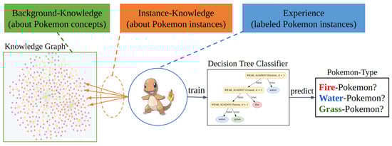
Figure 1.
The three main components of the investigated system. This work aims to use and optimize the MINDWALC node classifier for the following specific use-case system. The most important idea is to divide the given graph on which MINDWALC operates into three components: first, the inner background knowledge (green), which describes how domain-specific concepts are related to each other; second, the experience (blue), which is represented by labeled instance nodes (nodes to classify). third, the instance knowledge (orange), which is represented by specific relations which connect each node instance with multiple concept nodes from the background knowledge graph. The idea is to classify the node instances of such a system using a MINDWALC decision tree classification in order to generate human-interpretable decision trees during training.
The most important point of our use case setting is that the processed graph is always divided into three specific components. Each component has a very specific meaning and represents one essential subprocess of decision-making:
- Background Knowledge:The background knowledge is the inner part of the KG and describes how different domain-specific concepts are related to each other. As exemplified in the Pokemon domain, it describes how different Pokemon concepts (properties, abilities, movesets, teams, etc.) are related to each other. In the medical domain, background knowledge could be a medical ontology, which describes how different medical terms are related to each other. Since the background knowledge graph defines the fundamental knowledge and rules of the present domain, it is important that the content of this graph is free of false statements to avoid wrong conclusions during classification tasks.
- Experience:The amount of our labeled instance nodes represents the experience of our classification system. Therefore, in our case, the more labeled Pokemon nodes (instances) are known, the more experience our classification model obtains, which usually has a positive impact on its classification accuracy.
- Instance Knowledge:Instance knowledge represents the knowledge about each instance, e.g., which Pokemon instances have which abilities, belong to which groups, or have which weaknesses and strength. Instance knowledge is represented by the first relations that connect each Pokemon node to the actual background knowledge graph. In practice, the instance knowledge might not always be perfectly complete and correct, since the knowledge about each instance usually has to be retrieved in some way and this might not always work perfectly. As an example in medicine, patient cases are instances due to unique information (instance knowledge) about the patient. Instance knowledge about a case might not always be detailed enough to be able to make a reliable diagnosis.
If we think about how we humans make decisions, it is entirely possible to make purely intuitive decisions, without using any background knowledge and only based on experience and sufficient instance knowledge. However, our reliability in decision-making usually benefits from utilizing background knowledge that has been acquired during education or looked up in reference articles.
After we clarified the structure and meaning of the three knowledge graph components, we can now explain how we use them together with machine learning to classify certain node instances and generate decision trees. As shown in Figure 1 from left to right, we first need a background knowledge graph; then, we collect labeled instances and instance knowledge in order to connect them with our background knowledge using meaningful relations. We then train a decision tree-based node classifier that uses the instance knowledge together with the deeper hidden background knowledge to predict the labels of the instances. After that, we are especially interested in examining the trained decision trees to obtain an impression of how human-comprehensible they are.
For our use case setting, the MINDWALC node classification approach does perfectly fit, due to its ability to walk through the first instance knowledge layer into the deeper background knowledge in an interpretable way. It is particularly interesting how deep the classifier walks into the KG to make decisions. Decisions that are based on walks larger than one step walk into the area of the background knowledge. Such decisions are no longer made purely intuitively, based on experience. They also use logical thinking and combined conclusions. The deeper the walk, the longer and more complex the combined conclusion. Our key motivation to use this system is the clear division into background knowledge, instance knowledge, and experience, as well as the fact that the decision-making is interpretable and human-comprehensible.
2.2. Examined Knowledge Graphs
To investigate how different approaches perform on different knowledge graphs and node classification tasks, three different Pokemon-related knowledge graphs—one synthetically generated medical knowledge graph, and three real-world datasets—were used for testing. Table 1 provides an initial overview of the properties of the respective graphs. More detailed information on each graph can be found in Section 2.2.1, Section 2.2.2, Section 2.2.3, Section 2.2.4 and Section 2.2.5.

Table 1.
Properties of examined knowledge graphs. Node and relation count of all seven multi-relational graphs which have been examined in this work. Train-test entities indicates how many labeled nodes are available in the graph, which are used to train and test different MINDWALC node classifiers.
2.2.1. GottaGraphEmAll Pokemon Graph
As an example of a property-based graph structure, the GottaGraphEmAll graph was used. It was provided as a Neo4J graph database by [19]. As we can see in the schema of the graph (Figure 2), this graph describes the characteristics the Pokemon have among each other (abilities, moves, weaknesses, and strengths against types). We call this graph a property-based knowledge graph because this graph mainly describes which properties each Pokemon has and how the properties and/or Pokemon are related to each other.
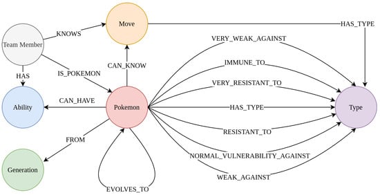
Figure 2.
The schema of the knowledge graph GottaGraphEmAll. The schema of the Pokemon graph GottaGraphEmAll. As we can see, this knowledge graph describes how different Pokemon are related to different Pokemon types, team members, abilities, generations, and moves.
2.2.2. TreeOfLife Pokemon Graph
Some knowledge graphs are based on a hierarchical structure, where each node can be divided into multiple subnodes, which results in a tree-like topology. Especially many medical terminologies, such as Kidney Biopsy Codes (KBC) [20], Unified Medical Language System (UMLS) [21] or Snomed CT [22] are based on hierarchical structured medical terms, so that they can be represented by an incomplete tree. As an example for a hierarchical-based knowledge graph for the Pokemon use case, the phylogeny and evolutionary tree of life graph, computed and published by Shelomi et al. in [23], has been converted into a Neo4J graph. As shown in Figure 3, the tree of life Pokemon graph assigns each Pokemon node (pink leaf nodes) to multiple sub-Pokemon groups (blue nodes).
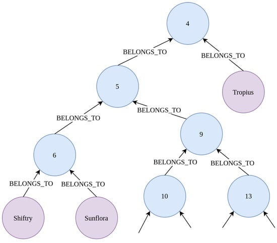
Figure 3.
Small part of the tree of life Pokemon graph. As we can see, the tree of life Pokemon graph has a tree-like structure. Each Pokemon node (purple nodes) is a leaf of the tree and belongs to multiple PokeCategory nodes (blue nodes, named with random category numbers). This tree of life graph was generated in [23] and the Pokemon grouping is based on anatomical properties and other Pokemon attributes.
2.2.3. Combined Pokemon Graph
For another test, both previously mentioned graphs (Section 2.2.1 and Section 2.2.2) are joined to make one graph in order to investigate how well our improved version of MINDWALC performs on graphs based on multiple topologies. This is because, in practice, we might prefer such larger, joined graphs to utilize as much knowledge as possible in one single knowledge base. The only nodes that the two graphs have in common are the Pokemon nodes. When joining them together, care was taken to ensure that each Pokemon node existed only once in the resulting graph. Moreover, we removed each Pokemon node that did not exist in both graphs.
2.2.4. ProstateToyGraph
To carry out some experiments in a specialized medical domain, we created a custom graph that describes knowledge about prostate adenocarcinoma. To start, we first selected the concepts relevant for prostate cancer diagnosis from the Snomed CT ontology. We then expanded the knowledge contained in this graph by manually adding missing concepts and relationships, according to our pathological experience and reference books. The resulting knowledge graph is publicly available in our github repository. Table prostate-graph-1.3_log.xlsx, which is attached in the supplementary material, documents which relations and nodes were added.
Next, we generated several synthetic pathological cases. Each case is represented by one case node instance and belongs to one of the following diagnostic classes (detailed explanations about the meaning of these classes can be found in Section 3.3):
- adenocarcinoma (GP3-5)
- GP3 mimicker
- GP4 mimicker
- GP5 mimicker
Our medical specialists created one concept list for each class. Each concept list contains several concepts which typically occur in cases that belong to the corresponding diagnostic class. These lists can be found in the supplementary material of this publication (SyntheticInstanceGeneration1.1.xlsx). We implemented a script that generates 111 case node instances for each diagnostic class. Each generated case node was then randomly connected with 10 to 100 % of the concepts listed for the corresponding class, with relations of type DETECTED.
2.2.5. Real World Datasets
To test how our methods perform on real-world datasets, we used three different benchmark graph datasets, namely AIFB, BGS and MUTAG. All three datasets were also used in the original MINDWALC work by Vandewiele et al. [3] and are publicly available in a repository set up by Ristoski et al. [24]. Statistical information on these graph datasets can be found in Table 1.
The AIFB dataset describes how processes, researchers, departments, projects, and other entities of a research institution are related to each other. The classification task is to assign each researcher to one of multiple research groups.
The BGS dataset describes geological measurements of 146 rock units and the classification task is to predict which rocks are fluvial or glacial.
The MUTAG dataset comes from the biochemical field and describes 340 complex molecules. The classification task is to determine whether certain molecules are potentially carcinogenic.
2.3. Technical Overview of MINDWALC Decision Tree Classification
This Section provides an overview of the methodology of the MINDWALC algorithm. It covers MINDWALC’s functionality only superficially and provides a simple overview of its essential mechanics. More specific details can be found in the original work [3]. The diagram in Figure 4 shows the complete functionality of the MINDWALC decision tree classifier in simplified form. We have divided MINDWALC into the following three essential components/steps (I, II, and III):
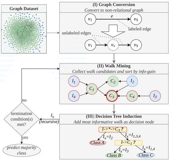
Figure 4.
Methodical overview of MINDWALC decision tree classification. (I) The MINDWALC data processing pipeline begins by converting a relational knowledge graph into a non-relational graph by transforming each relation into a node. (II) The second step is the primary concept of MINDWALC, which involves mining walks through the graph. Each walk starts from the node instances (, blue nodes) and proceeds through the graph until a certain target concept node (, green nodes) is reached. The information gain of each walk is calculated (see [3] for details). The most informative walk is used to generate the next decision tree node. (III) A binary decision tree is built recursively from top to bottom. Each decision node (yellow) splits the given instances into two groups based on whether they can complete a particular walk (right child) or not (left child). The notation in the decision nodes describes the corresponding walks that start at the instances I and end at a target node . All nodes in between can be any node and are marked with ∗, as defined in Formula (1).
2.3.1. Graph Conversion
As introduced in [3], MINDWALC expects a multi-relation directed KG, , as input. The vertices, , and the directed edges, , of G are labeled with a labeling function, ℓ. However, to reduce the complexity of the given graph, the first step of the MINDWALC data processing pipeline is to convert the given relational knowledge graph into a non-relational graph. For this, each relation, e, is simply converted into one corresponding node, , as visualized in Figure 4(I). This conversion can have certain disadvantages, which are discussed in Section 2.5 in more detail.
2.3.2. Walk Mining
The second component, (II), (Figure 4) represents the main idea of MINDWALC: collecting (mining) so-called (mind-)walks, w. Each walk starts at the node instances to be classified, I, and then searches for directional paths through the non-relational KG. As explained in [3], such a walk is defined by
where is the node instance (node to classify) from which the walk starts, l is the walking depth, and x is the target node, which is a concept node of the given KG. Therefore, w can be defined using a tuple .
This is how walk mining works: First, all possible walk candidates are collected, so that each walk candidate can be completed by at least one of the given instances. For each walk candidate, an information gain is calculated, based on which instances can complete the walk and which cannot (see [3], formula 4). In Figure 4(II), for example, all instances () that can reach the walk, , are marked in red. If, for example, all instances selected in red belong to the same class, this walk gets a large information gain value, accordingly.
2.3.3. Decision Tree Induction
In order to grow a binary decision tree, each decision node of the tree is generated recursively in a top-to-bottom manner. Each decision node represents the most informative walk and checks whether each instance can complete the given walk or not. This splits the instances recursively into the ones that can (right child) and cannot (left child) complete an informative walk, until one of three termination conditions is met (as defined in [3]). All left instances belong to the same class, a minimum amount of instances is left, or the maximum decision tree depth is reached).
Using MINDWALC with Other Classifiers
Vandewiele et al. also introduced the MINDWALC transformer, which essentially executes one single walk mining procedure to generate binary MINDWALC feature vectors, , for each i’th of n instances . describes which of the m available walks, , can or cannot be reached by . The extracted MINDWALC feature vectors can be passed to any classifier of choice; for example, random forest or logistic regression classifiers.
However, in this work, we are mainly interested in the decision tree classifier, since a visualized decision tree can be interpreted very well and intuitively by humans.
Algorithmic Properties of MINDWALC
As shown in [3], the computational complexity required to perform the walk mining (finding the most informative walks) depends linearly on three different parameters: , with the maximum allowed walking depth, d; the number of vertices, , in the graph; and the number of instances, .
Generally, decision tree induction algorithms such as CART [25] have a computational complexity of [26,27] with m as attribute count and n as the number of training instances (so ). The attribute count is given by the vector size of the given feature vectors, which, in our case, is the same as all possible walk candidates, which is [3]. Unfortunately, however, the MINDWALC decision tree classifier is currently implemented in a way in which the dataset is repeatedly re-evaluated each time the procedure is called (by recalling mine_walks(), see algorithm 4 in [3]). This increases the computational complexity to [27], which corresponds to in our case. However, to achieve a lower computational complexity, we can also use the MINDWALC transformer to first extract the MINDWALC feature vectors with costs of and then pass them on to a modern CART-based decision tree model that adds costs of . Since is the dominant term of the sum , we obtain a resulting complexity of , which corresponds to , using MINDWALC’s notation.
Another well-known property of decision tree classifiers is that they are prone to overfitting due to their discriminative and greedy behavior, whereby locally optimal decisions are made at each decision node. [28]. However, this can be partly compensated by applying pre- and post-pruning or with dual information distance (DID) [29], as an example.
2.4. Extending Walking Strategies with Flexible Walking Depths
As already mentioned in the conclusion of the MINDWALC manuscript [3], the standard walking strategy, as defined in Equation (1), can have disadvantages in certain cases, which is why we investigated alternative walking strategies in this work. During our investigations, we have recognized that it can, in some cases, be difficult to find similarities between instances that belong to the same class with this type of walk, especially when operating on hierarchical, tree-like structured knowledge graphs. Such graphs often appear in the medical domain, as they are regularly based on hierarchical terminologies like KBC [20], UMLS [21], or Snomed CT [22].
In such situations, leaving out the fixed walking depth, l, can help to find more similarities between the instance feature vectors. The omission of a fixed depth value is called flexible walking depth and means that only the target node, x, must be reached, regardless of the walking depth.
Figure 5 shows a simple example in which instance similarities can only be found if we allow flexible walking depths. This graph consists of two instance nodes, , and two concept nodes, . To construct two feature vectors, , for both instances, we first have to search for all possible walk candidates. As we can see (Figure 5, walk candidates), there are three walks of flexible depth, , (orange) and two of flexible depth, (purple). In this graph, and have only one walk candidate in common, which is , a walk of flexible depth.
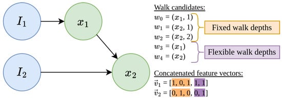
Figure 5.
Example of MINDWALC’s feature extraction based on walks. Example of how we can construct binary feature vectors, , for each i’th instance node, , using different walking strategies. describes which of m available walk candidates, , can or cannot be executed by . In this case, we can find different walk candidates, , in the given graph. The first three walk candidates, are walks with fixed walking depths, where fixed walking depths, l, are defined. The last two walk candidates, , are walks with flexible walking depth, where only a required target node, x, is defined. Therefore, there are three options to construct the feature vectors: We can either use walks of fixed (orange) or flexible (purple) walking depth, or, as done in this case, we can combine both walking strategies together into one large feature vector. In this case, and have only one feature, , in common, which is a walk of flexible depth.
We assume that there is no walking strategy that works best. It probably depends heavily on what kind of knowledge graph is being processed, as well as on the given classification problem. We can also use both walking strategies together (combined walking strategy) by collecting flexible and fixed walks and then concatenating them into one feature vector, as shown in Figure 5. Obviously, we will then have significantly larger feature vectors. How different walking strategies behave on different graphs is examined in Section 3.2 in more detail.
2.5. Taking Relations into Account Using Relation-Tail Merging
To reduce the system complexity, MINDWALC is designed to operate on a directed, non-relational graph, which means that it is not able to consider that there are different relation types in the given knowledge graph. To be able to consider relations, MINDWALC converts each relation of a given relational graph into one node, as mentioned in [3]. For this, each head-relation-tail triple, (h)-r->(t), is converted into (h)-->(r)-->(t), whereas --> are non-relational, directed edges. Although this method is simple and efficient, it has the limitation that each node that was previously a relation will always have exactly one incoming and one outgoing directed edge. This limitation can, in some situations, make it difficult for MINDWALC to find enough meaningful similarities between instances during the feature extraction process. As explained in Section 2.4, the feature extraction of MINDWALC is based on searching the graph for informative walks. Each walk, w, starts from the instance nodes, I, and ends at a certain target node, x, which is located at a certain depth, l, in the KG. Now, if we look at the example in Figure 6A, we have two Pokemon nodes which have the following similarity: both are weak against fire. Now, after converting each relation into one node, we can see that, according to all possible walks, the only thing the Pokemon nodes have in common is that they are both somehow related to Fire (with walk w=(x,l)=(Fire,2)). Walks like w=(WEAK_AGAINST_0,1) are not very informative, because they represent the statement that a Pokemon is weak against an unknown node. They do not provide any information about what this Pokemon is weak against. However, we can combine multiple walks in our decision tree to construct more complex statements, but it is not possible to find one single walk that is capable of describing that both Pokemon are weak against fire.
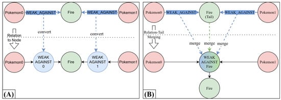
Figure 6.
Example of relation-tail merging. (A) The previous method for considering relations using relation-to-node conversion, as proposed in [3]. (B) In our new method, called Relation-Tail Merging (RTM), we merge all relations of the same type into their common tail node. As we can see in this particular example, with method B, the overall size of the resulting non-relational graph becomes smaller compared to method A (one node and two relations less). Much more importantly, we obtain more meaningful relation-modified target nodes (here: WEAK_AGAINST_Fire).
To solve this issue, we introduce an alternative graph conversion method called Relation-Tail Merging (RTM). As the name suggests, this method basically merges a set of type-identical relations into one individual tail node. An illustrative example of the relation-tail merging process is shown in Figure 6B.
The process of RTM works as follows: First, a tail node is selected, t, as well as a set of relations of identical type, r, where the topological form (*)-r->(t) is given. The process of relation-tail merging then involves inserting a new node, , so that (*)-r->(t) turns into (*)-->(rt)-->(t). The new directional edges, -->, are now typeless, and the new inserted node, , represents a relation-modified node and is named accordingly in the form <type_of_r>_<name_of_t>. Thus, in the given example in Figure 6, all -WEAK_AGAINST->(Fire) connections are merged into the new relation-modified node WEAK_AGINST_Fire. As we can see in Figure 6, RTM also creates fewer additional nodes to the KG than the relation-to-node conversion method (A). In this case, we end up with one node and two relations less.
With relation-tail merging, the entire graph can be converted into a non-relational, but fully relation-modified, directional graph by applying relation-tail merging repeatedly to the given KG until each relation is resolved and represented by relation-modified nodes.
In cases where all existing relations, r, which point to t, are of the same relation type, the relation-modified statement is always the same for all -r->(t). In such cases, we can perform relation-tail merging in the form (*)-r->(t) to (*)-->(rt), so that t is overwritten by . As a result, no additional relations or nodes are generated.
3. Results
In the results section, we first compare MINDWALC with a much simpler frequency-based decision tree classification approach in Section 3.1 to investigate when and how MINDWALC utilizes the background knowledge stored in a KG.
Secondly, in Section 3.2, different walking strategies (as proposed in Section 2.4) are tested on three different structured Pokemon graphs.
Thirdly, in Section 3.3, we apply and compare all our proposed methods in a medical scenario using our synthetic graph ProstateToyGraph (as introduced in Section 2.2.4).
Lastly, in Section 3.4, we compare how different configured MINDWALC classifiers perform on multiple real-world graph datasets (as introduced in Section 2.2.5).
3.1. Training Decision Trees with and Without Background Knowledge
In this Section, we examine in more detail when and how MINDWALC utilizes the background knowledge stored in a KG to solve a given classification problem.
To examine this, we used the GottaGraphEmAll Pokemon graph (see Section 2.2.1) and formulated the following classification task. The classification task is to predict one of three Pokemon types (Fire, Water, or Grass) of each Pokemon node based on individual weaknesses and other Pokemon properties and relations between them. To make the task not too easy, we removed each relation of type -HAS_TYPE-> from the graph. Moreover, we applied relation-tail merging to the KG (as proposed in Section 2.5), as MINDWALC would otherwise not be able to distinguish whether a Pokemon is weak or strong against an element.
In this classification task, it is very likely that the most discriminative features are strength- or weakness-related nodes, such as the relation-modified nodes WEAK_AGAINST_Fire or RESISTANT_AGAINST_Ice. These nodes are in the immediate neighborhood of each Pokemon node. This means that the background knowledge, which is hidden deeper in the Pokemon knowledge graph, is not necessarily needed to predict the Pokemon type of a Pokemon node. Therefore, we also look at the performance of a simple decision tree classifier, which does not have access to the deeper background knowledge. We call this node classifier a “frequency-based” decision tree node classifier because it basically converts the closest neighborhood of the Pokemon nodes into binary feature vectors and passes them to a conventional decision tree classifier. In contrast to the frequency-based decision tree classifier, the prediction of the MINDWALC decision tree classifier is based on walks that lead deeper into the background knowledge.
Since the given Pokemon graph GottaGraphEmAll is perfectly complete, the classification task might be very easy to solve for both classifier approaches and might deliver 100% accuracy. To investigate how both classifiers behave under more difficult circumstances, we gradually increase the classification difficulty by simulating increasingly incomplete knowledge about the Pokemon nodes. We implement this by gradually deleting a greater percentage of the relations that point away from the Pokemon nodes. We call this process instance knowledge degradation, since it only destroys instance-specific knowledge about the Pokemon nodes, while the deeper hidden background knowledge, which describes how all Pokemon-properties are related to each other, remains undamaged. During instance knowledge degradation, we made sure that every Pokemon node always keeps at least one of its outgoing relations. Otherwise, we could obtain featureless Pokemon nodes, which are completely detached from the whole KG.
Figure 7 shows the results of our test. Each measuring point of the three curves in this figure was obtained by a 10-fold cross-validation. This means that each y-value is the mean value of 10 training and test runs. Standard deviations are also shown using semitransparent coloring. Both diagrams, A and B, show on the x-axis what percentage of Pokemon relations have been destroyed (using instance knowledge degradation, as explained above). The classification performance of both classifiers has been measured with the F1-score and can be found in the upper-left corner of the figure (A). The complexity of the decision trees produced is measured with the decision node count of the decision trees produced during training and can be found in diagram B. We used the decision tree node count as a complexity measure, since it is a measure for the overall decision tree size, which can also be interpreted as a measure of how complex a decision tree is.
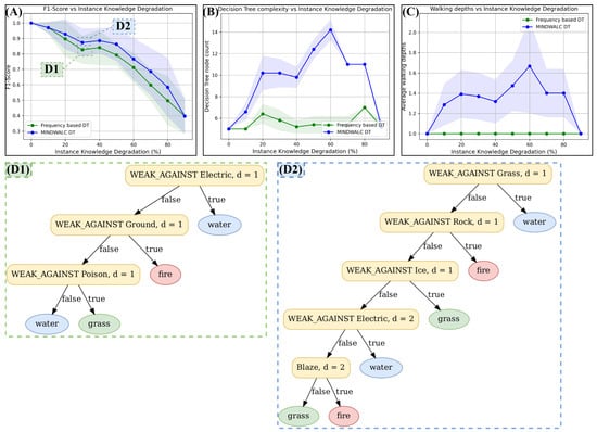
Figure 7.
Comparison of a frequency-based decision tree classifier with MINDWALC. In this experiment, the instance knowledge (defined in Section 2.1) undergoes a gradual degradation through the random removal of 10–90% of its relations. Subsequently, decision trees are trained for each resulting, less comprehensive instance knowledge, employing either the node frequency-based method (green curves) or the MINDWALC algorithm (blue curves). (A) The 10-fold cross validated F1-scores of the resultant decision trees are then graphically represented against the level of instance knowledge degradation. (B) For the resulting decision trees, the complexity is calculated and plotted against the grade of degradation. (C) For the resulting decision trees, the average used walking depth is calculated and plotted against the grade of degradation. (D1,D2) Two examples of generated decision trees are shown. (D1) shows one graph generated by the frequency bases approach, and (D2) shows a graph generated by MINDWALC. Conclusion: we can observe that, compared to the frequency-based decision tree classifier, as soon as we reduce the instance knowledge, the MINDWALC decision tree classifier starts to walk deeper into the knowledge graph (C), has a higher classification accuracy in most cases (A), and its average decision tree complexity becomes significantly higher (B).
We also measured how deep the generated decision trees walk into the KG. For this, we calculated the average walking depth by simply iterating through each decision node of all 10 trained decision trees (from the 10-fold cross-validation) and calculating its average walking depth. The average walking depth values are shown in Figure 7, diagram C. For each measurement point from all three diagrams, A, B and C, we also calculated the standard deviation and visualized it with semitransparent coloring.
As expected, diagram A shows that both approaches, MINDWALC as well as the simpler frequency-based approach, achieve the best possible classification performance of 1.0 for the F1-score as long as there is no instance knowledge degradation (see diagram A, at 0% degradation). Moreover, we can see in diagram C that the MINDWALC decision tree classifier does not make any use of the deeper background knowledge, as long as there is no degradation of the instance knowledge, since the average walking depth is 1.0 at 0% degradation.
As soon as the instance knowledge degradation is ≥10%, we can observe that, compared to the frequency-based decision tree classifier, the MINDWALC decision tree classifier achieves the following:
- starts to walk deeper into the KG (diagram C).
- has a higher classification accuracy in most cases (diagram A).
- its average decision tree complexity increases significantly (diagram B).
The fact that MINDWALC’s classification performance becomes better than the frequency-based classifier, as soon as it starts to use deeper walking depths, shows that MINDWALC is in fact able to compensate for weak instance knowledge by utilizing background knowledge.
The next question is as follows: Does MINDWALC utilize the background knowledge in a human-understandable way? To investigate this question, we can take a closer look at some of the decision trees generated, as shown in Figure 7(D1,D2), where both decision trees are generated at an instance knowledge degradation of 30%. Figure 7(D1) is generated with the frequency-based decision tree and Figure 7(D2) is generated with MINDWALC. In the decision tree shown in Figure 7(D2), the decision node WEAK_AGAINST Electric,d=2 checks whether the Pokemon to be classified can reach the node WEAK_AGAINST Electric in two steps (d = 2). This means that the Pokemon’s pre-evolution is checked here to see whether it is weak against electricity or not. If that is the case, the decision tree predicts a water Pokemon. This implies that MINDWALC has learned that the pre-evolutions of Pokemon are often of the same Pokemon type. It can be interpreted as background knowledge, which is utilized to make better decisions when some instance knowledge is missing. The same counts for the decision node Blaze,d=2. Here, the model checks whether the pre-evolution (d = 2) has the Pokemon ability Blaze. Indeed, this is a typical fire Pokemon attack, which is what the model predicts if this decision node is fulfilled.
3.2. Comparing Walking Strategies on Different Pokemon Knowledge Graphs
In the previous section, we demonstrated that decision trees produced by the MINDWALC algorithm outperform semi-manual node selection in terms of classification accuracy by utilizing walks into the given KG. In this section, we examine how different walking strategies of the MINDWALC approach perform on knowledge graphs that differ in their topology.
For this, we use three different Pokemon-related knowledge graphs. The first, the GottaGraphEmAll graph used above, has a property-based structure with a less hierarchical order (see Figure 8A). The second graph is the evolutionary Pokemon graph, calculated by Shelomi et al. in [23], and has a pure hierarchical tree-like structure (Figure 8B). Lastly, we combine both graphs to form one large Pokemon KG (Figure 8C). Please refer to Section 2.2 for more details on the graphs used. The classification task is to predict the Pokemon type (fire, water, or grass) of each Pokemon node in the graph.
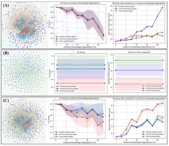
Figure 8.
Decision tree performance and complexity of different walking strategies on different graph types. The three different walking strategies (red, fixed; green, flexible; blue, combined walking depths) are tested on three different graph topologies (rows A–C) with regard to classification performance (middle column) and decision tree complexity (right column). Classification performance and complexity are measured in the same way as in Section 3.1. (A) The property-centered GottaGraphEmAll graph, as introduced in Section 2.2.1. Here, no significant differences can be observed with regard to the classification performance. However, the complexity of the combined walking strategy increases very rapidly as soon as instance knowledge degradation occurs . (B) The evolutionary, hierarchically structured Pokemon graph, as introduced in Section 2.2.2. As we can see, the flexible walking depth (green curves) classifies much better on this graph compared to the other walking strategies. (C) The combined graph. In this case, we joined graph (A) and (B) together to produce a larger graph based on hierarchical- and property-like structures. In this case, the best option seems to be the combined walking strategy (blue), according to its classification performance, as well as its small decision tree complexity.
Moreover, the following three walking strategies are tested together with a MINDWALC decision tree classifier: First, we used the fixed walking depth, as introduced in [3] (Figure 8, red curves). Second, we applied flexible walking depths, as proposed in Section 2.4 (Figure 8, green curves). The third walking strategy is a combination of flexible and fixed walking depth (Figure 8, blue curves).
As in the previous section, we applied instance knowledge degradation, starting from 0% and increasing up to 90% to simulate better to worse instance knowledge, while keeping the background knowledge about connections between the Pokemon properties untouched. It is important to note that the instance knowledge degradation was applied to the knowledge graphs, except for the hierarchical Pokemon graph (B). It is not possible to apply instance knowledge degradation to this graph because each Pokemon node has only one direct connection (relation) to the KG. This connection must not be removed, otherwise we immediately obtain featureless Pokemon nodes that do not have any connection with the KG. For a better overview, we have visualized the single measurement points on the hierarchical graph as a straight curve.
Regarding the metrics measurement techniques, each measurement point of each curve in Figure 8 is again the averaged result of a single 10-fold cross-validation. We used the F1-score to measure the classification performance of each configuration (Figure 8, center column), and we again used the decision tree node count to obtain an impression of how complex and large the generated decision trees are (Figure 8, right column).
On the property-based graph (A), there is no significant difference between each walking strategy. The flexible and fixed approaches, as well as the combined walking strategy, show a similarly reduced performance with increased instance knowledge degradation, whereby the decision trees of the combined walking strategy become significantly more complex than the other ones. On the hierarchical evolutionary Pokemon graph (B), the fixed walking strategy (red) classifies significantly worse than the other walking strategies. Compared to the fixed walking depth, the flexible walk has an F1-score that is around 0.5 higher. The combined walk also performs significantly better than the fixed depth but slightly worse than the flexible depth. As explained in Section 2.4, the flexible walk is, in most cases, the best method to find informative similarities in tree-like structured graphs, which is obviously why the flexible walk has performed best. However, if the flexible strategy resulted in such good classification results, why did the combined strategy perform worse on this purely hierarchical graph? To investigate this in more detail, we looked at some example trees, generated with the combined strategy, and discovered that flexible walks have been selected in most cases, but not always. In some rare cases, especially at the very last decision node of a decision tree, fixed walks have been used. Thus, apparently, as soon as there were fewer instances during the decision tree growing process, fixed walks received the strongest information gain. However, this does not seem to be the most optimal decision in the test dataset.
Again, on the combined Pokemon knowledge graph (C), the flexible walking strategy and the combined strategy outperform the fixed walking depth as soon as the instance knowledge degradation becomes greater than 30%. In this case, both walking strategies show stronger classification performance while generating even less complex decision trees.
3.3. Tests on a Medical Toy Dataset
In this Section, we will test how our methods perform on a simulated clinical application. For this, we first created a toy knowledge graph about prostate carcinomas, as introduced in Section 2.2.4.
As explained in detail in Section 2.2.4, we generated 444 pathological cases as instances. In the simulated scenario, several features were detected for each case, e.g., during microscopy of tissue section specimens (for example, features like “adenosis”, “hyperchromatic nuclei with nucleoli”, or “solid growth pattern”; refer to Section 2.2.4 for more details). Each node instance is represented by a corresponding case node that is interwoven with the prostate knowledge graph according to the detected features of the case. For this purpose, each feature of a case is connected to the corresponding concept node of the prostate knowledge graph with one DETECTED relation (e.g., (case)-DETECTED->(adenosis)).
To add more noise and realism to our clinical scenario, we also simulated different specific terms which were used to describe the same features. Such situations could arise in practice due to the different ways pathologists describe certain patterns individually. For example, one pathologist may prefer to use the term “adenosis”, while another may prefer to use the narrower term “fibrosing adenosis”. For this, randomly narrowed subterms were inserted, with a probability of 50%, during the instance interweaving process (e.g., (case)-DETECTED->(fibrosing adenosis)-ISA->(adenosis)).
Each case is labeled with one of the following diagnostic classes:
- 111 × adenocarcinoma (GP3-5)
- 111 × GP3 mimicker
- 111 × GP4 mimicker
- 111 × GP5 mimicker
As we can see, only 25% of the cases given are in fact prostatic adenocarcinoma (with grade Gleason Pattern (GP) 3 to 5). All other cases might appear as malignant cancer at first glance, but upon closer analysis, they are not because they show one or more benign mimics of prostate adenocarcinoma (e.g., as listed in [30]). These cases are labeled accordingly with GP3 mimicker, GP4 mimicker or GP5 mimicker.
In a real-world clinical setting, perfectly complete instance knowledge (knowledge about cases) might appear very rarely because we never know every relevant fact about each case. Therefore, we again applied instance knowledge degradation, in the same way as explained in Section 3.1, to produce the classification performance diagram (A) and decision tree complexity diagram (B) in Figure 9.
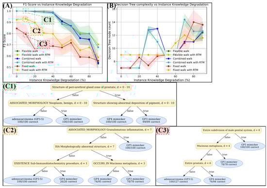
Figure 9.
Test results on the knowledge graph ProstateToyGraph, as introduced in Section 2.2.4. As introduced in Section 3.1, we applied instance knowledge degradation to simulate more or less available case informations (x-achsis in (A) and (B)). In diagram (A), we can see that the fixed walking depth strategy initially classifies worst (red curve), but improves significantly with RTM (orange curve), especially if enough instance knowledge is available (0–40% degradation). For flexible and combined walking strategies, another significant performance jump is observed, though the improvement is marginally enhanced by RTM. According to diagram (B), the complexity of decision trees generated by flexible and combined strategies is sometimes higher than those generated by the fixed strategy. (C1–C3) shows some examples of the produced decision trees. Some decisions by these trees were deemed comprehensive by our specialists. For example, “structure showing abnormal deposition of pigment” in (C1) indicates seminal vesicles, which are indeed a mimicker of GP 3. However, several decisions are less comprehensive and based on vague and broad concepts that are high in the Snomed CT hierarchy.
The following can be seen in the classification performance diagram (A):
In this scenario, the fixed walking depth performs worst (red). However, if RTM is applied, the performance of the fixed walking strategy improves significantly (orange), especially if a reasonable instance knowledge is given (0 to 40% instance knowledge degradation).
Another significant jump in classification performance occurs when we use the flexible or combined walking strategy. Both strategies perform very similarly, and RTM does not help as much as it does for the fixed strategy. However, it slightly increases the performance of the flexible and combined strategy as soon as the instance knowledge degradation becomes higher than 60%.
It is also notable that the decision trees generated by the flexible and combined strategy are sometimes much more complex or much larger than the ones generated with the fixed strategy (see Figure 9B, ).
Since we are also interested in the comprehensiveness of the trained decision trees, we applied a maximum tree depth of 4 to force MINDWALC to generate smaller and less complex decision trees. Each trained decision tree has been rendered to a pdf file and each one is publicly accessible in the provided github repository. In Figure 9(C1–C3), we show some decision trees that were particularly interesting to our specialists. As an example, an apparently comprehensive decision can be seen in (C1), bottom-right. Here, 99 GP3 mimicker cases have been classified using the concept “structure showing abnormal deposition of pigment”. This concept indicates a seminal vesicle (ejaculatory duct), which, in turn, is in fact a mimicker of GP 3 (see [30]). However, the general comprehensiveness of the decision trees was mixed; although some decisions made impressionable sense, several less comprehensive decisions can be found, such as “ISA Morphologically abnormal structure” (C2) or “Entire prostate” (C3). These concepts are located very high up in the hierarchical terminology of Snomed CT (close to the root concept of Snomed), which is based on very vague and broad concepts.
3.4. Tests on Real-World Datasets
In this Section, we compare how our introduced MINDWALC optimizations (new walking strategies and RTM) perform on real-world datasets and how they compare to other node classification methods. For testing, we used the AIFB, the BGS, and the MUTAG datasets. Detailed information on these datasets can be found in Section 2.2.5. To obtain an impression of how MINDWALC performs compared to other state-of-the-art node classifiers, the accuracy scores of a R-GCN [9] and a RDF2VEC [10] node classifier were used. Each tested MINDWALC configuration consists of the following:
- one of four different MINDWALC classifiers;
- one of our three introduces walking strategies;
- and with RTM switched off or on.
In Table 2, fix stands for fixed walking depth, flex for flexible walking depth and both for the combined walking strategy. Activated RTM is denoted as “+ rtm”. For the different MINDWALC classifiers, we used the MINDWALC tree (tree), the MINDWALC forest (forest), and two different variants of the MINDWAC transformer, denoted as transform_lr and transform_rf in Table 2. transform_lr denotes a MINDWALC transformer with logistic regression as a classifier, and transform_rf denotes a MINDWALC transformer with random forest classification.
Table 2.
Accuracy comparison of different MINDWALC configurations on real-world datasets. Averaged accuracy scores of different configured MINDWALC node classifiers on the AIFB, BGS, and MUTAG datasets. This comparison has also been performed in the previous MINDWALC paper [3]. Here, we added our two new walking strategies (flexible and both), as well as RTM, to the tests. Overall, the results are very mixed and there is no particular MINDWALC configuration that works best on all three datasets.
Table 2 lists the accuracy scores achieved with the configurations mentioned above. It is divided into three subtables—one for each dataset (AIFB, BGS and MUTAG). Each test accuracy score is composed by the average value and standard derivation value of 10 training runs. For each run, simple grid search-based hyperparameter tuning was performed in the same way as in the original work by Vandiele et al. (see [3] (p. 9)). The accuracy scores shown for R-GCN and RDF2VEC are taken from [9].
Overall, the results of this experiment are very mixed and there is no particular MINDWALC configuration that works best on all three datasets. On the AIFB dataset, R-GCN performs about 5% to 7% better than MINDWALC. However, on BGS and MUTAG, the best MINDWALC configurations perform about 4% to 5% better than R-GCN and RDF2VEC.
- Results on AIFB dataset:
- On the AIFB dataset, the MINDWALC forest classifier is the best performing MINDWALC configuration, with up to 90.83% accuracy. Here, fixed and flexible walking depths perform noticeably better than the combined walk (about +3% better). The MINDWALC decision tree classifier seems to benefit from the two new walking strategies, as flexible and combined walks are about 3% to 4% better than the fixed walk. Relation-tail merging also seems to help here, albeit less significantly, with an increase in accuracy of around 1% to 2% compared to the fixed walk.
- Results on BGS dataset:
- Here, the MINDWALC transformer, together with a random forest classifier (transform_rf), performed best, with an accuracy score of 93.10% on the fixed and combined walking strategies. On the BGS dataset, all tested MINDWALC classifiers seem to harmonize particularly poorly, together with the flexible walking strategy, according to the lower accuracy scores in the flex row.
- Results on MUTAG dataset:
- On the MUTAG dataset, the MINDWALC forest classifier achieved the best classification accuracy score (77.5%) using the combined walking strategy and activated RTM. Furthermore, it is noticeable that both MINDWALC transformer-based classifiers perform significantly worse with the flexible walk than the MINDWALC tree and forest.
4. Discussion
4.1. Expected Challenges on Real-World Datasets in Medicine
It is important to mention that most of our evaluation datasets are synthetic toy datasets, which could obviously differ from real-world datasets. In particular, our Pokemon datasets might be unrealistically perfect regarding background knowledge and instance knowledge. Real-world medical datasets could be significantly noisier, incomplete, and could even contain wrong information or contradictions. We assume that the comprehensiveness of the generated decision trees strongly depends on how complete, correct, and precise the given KG is and how much knowledge it contains about the given classification problem. We have already observed this correlation in our tests: The Pokemon graph, which is perfectly modeled for the given classification problem, generated decision trees that were quite comprehensible in most cases. In contrast, our medical toy dataset produced less comprehensive decision trees. The medical toy dataset is based on Snomed CT, which does not contain much useful knowledge for prostate carcinoma diagnostics, since it is mainly a hierarchical terminology. We suspect that a knowledge graph that contains more connections between concepts related to prostate carcinoma would help to produce more comprehensive decision trees. However, obtaining a perfectly modeled background knowledge graph to solve real-world pathological domain-specific problems seems to be unlikely. At this point, we were unable to find any freely available high-quality knowledge graph or ontology that fit well enough for topics in which our pathologists are specialized.
Next, we discuss the impact of low-quality instance knowledge on the system. We experienced that incomplete instance knowledge can be compensated as long as a well-fitting high-quality knowledge graph is given. With our experiments, we were able to demonstrate this well in Section 3.1 by applying instance knowledge degradation. However, this gap-filling mechanism only works if a minimum amount of instance knowledge and a high-quality knowledge graph are available.
Another point to consider when using MINDWALC in real-world medical scenarios is the expected computational challenge. As discussed in “Algorithmic Properties of MINDWALC”, the computational complexity of an optimal MINDWALC decision tree classifier is . Thus, the costs depend log-linearly on the instance count, and linearly on the maximum walking depth, d, as well as the node count of the graph, . This means that the node count of the given graph has a greater impact than the training data count. Another very efficient option to reduce computational complexity is to apply a maximum decision tree depth, . This not only reduces the computational complexity to , it also helps to produce smaller and less complex decision trees, although the classification performance decreases. Although our proposed walking strategies generate different amounts of walk candidates, the O-notation of its computational complexity remains the same for each strategy ( possible walk candidates).
In this work, we used relatively small datasets (with respect to instance count and KG size) for very self-contained tasks to avoid long computation times and to facilitate evaluation and debugging. Therefore, one 10-fold cross-validation could be performed on mid-range computers in about 5 to 10 min and it was not necessary to use large computing resources. However, in a real-world applications, stronger computing resources might be necessary because many more diagnostic-labeled cases are needed to add as much experience as possible to the system. In addition, it would be necessary to use a much larger knowledge graph to cover knowledge about all topics that are treated at the corresponding institute. In addition to the operation of a knowledge graph database and regular decision tree training, tools are required that automatically interweave each case with all detected graph concept nodes. For example, this could be done with Named Entity Recognition (NER) tools which extract entities/concepts from case reports.
4.2. MINDWALC Optimizations
The MINDWALC algorithm, published by Vandewiele et al. in 2020 in [3], mines the most informative or discriminative walks in a graph. In this work, two new walking strategies are designed and tested together with the original walking strategies. In particular, a flexible walking length has been added, where the length of a walk between the starting node and the target node can have any depth that is smaller than the maximum walking depths. This flexible walking depth has been compared to the original fixed walking depth and a combination of both. Based on our test on two Pokemon knowledge graphs that differ by their general structure (property-centered vs. hierarchical-based), we could show that the walking strategy needs to be adapted to the graph. For a flat, property-based, nonhierarchical graph like the GottaGraphEmAll graph, there is no significant difference with regard to the walking strategy. Here, for the sake of saving computational effort and to keep the resulting decision tree complexity small, a fixed walking length should be used.
According to our tests, the flexible and the combined walking strategies are advantageous for graphs based on a hierarchical, incomplete tree-like structure, such as the Pokemon evolutionary graph, the combined Pokemon graph, and the prostate toy dataset. In the medical domain, this is probably the graph structure to be expected, as diagnosis systems and ontologies naturally inherit a hierarchy. In kidney tissue, for example, the first step is to analyze in which compartment of the parenchyma changes occur, and then these changes per compartment are further classified (as in the KBC terminology [20]).
What we could not yet clarify in detail is when to prefer the combined walking strategy over the flexible one or vice versa, as both strategies performed very similarly in our tests. However, if the structure of a given graph is not well known, the combined walking strategy might be the best choice. But, it should be noted that this method results in longer feature vectors and, consequently, longer computation times, even though it does not have a significant impact on the computational complexity.
It can be said that flexible walks are very unspecific walks because only a destination node, x, is specified, while nothing else is specified about how to reach the destination. In contrast, fixed-depth walks are more specific walks because, in addition to the destination node, a permitted fixed walking depth is also specified. One could also consider defining a third walking strategy that is even more specific than the fixed-depth walk. For example, we could specify that in addition to a destination node, x, another waypoint node, a, must be passed. However, we decided against implementing and testing such a walking strategy for the following reasons: First of all, with more specific walks, the combination possibilities increase, which means that even more walking candidates are found and the feature vectors become even longer and potentially more sparse. Secondly, more specific walks already indirectly exist in our system, since the decision tree is able to conjugate multiple walks. As an example, the walking sequence could also be represented by a conjunction of the walks and , which can be represented by a decision tree.
Moreover, walks where the last k target nodes are specified, with walk sequences like , would obtain the exact same information gain as . This is because, if the sequence exists in the graph, then the exact same instances that reach will also reach . Thus, the usage of walks of type is not necessary, since we could also use instead.
In addition to the walking strategies, there is also the need to discuss the method by which a given multi-relational graph is converted into a non-relational graph so that MINDWALC can operate on it. From our point of view, the proposed method relation-tail merging comes only with advantages, compared to the previous relation-to-node conversion method. Firstly, fewer additional nodes and edges are generated, as explained in Section 2.5. Secondly, the created relation-modified nodes represent concepts that have been contextualized by a relation, which improves the interpretability of such nodes. Thirdly, relation-modified nodes can be very important for decision-making. This was the case in our Pokemon-type classification task, where we urgently needed this conversion to be able to distinguish whether a Pokemon was weak or strong against an element, such as fire (as explained in Section 2.5).
5. Conclusions and Outlook
In summary, we successfully developed and tested the following methods to improve MINDWALC for usage in instance and background knowledge-separated knowledge graphs: First, we used relation-tail merging as an alternative graph prepossessing method to add relationship-modified nodes to the resulting non-relational directed knowledge graph. This method not only reduces the overall graph size on which MINDWALC operates. We were also able to show that this method improves MINDWALC’s ability to find more meaningful similarities between Pokemon instances in our Pokemon dataset.
Second, we introduced walks with flexible walking depths, which, as expected, performed significantly better on hierarchically and incomplete tree-like structured graphs.
Third, we introduced a combined walking strategy, where we simply used both flexible and fixed walking depths to extract the features from the graph. This may be the most flexible strategy, but does generate much longer feature vectors, which might be one reason why it did not always perform best.
Additionally, we were able to show that MINDWALC is able to generate comprehensive decision trees and to utilize background knowledge to replace missing instance knowledge, as long as a high-quality knowledge graph is given. This is an important ability in our use case, as in pathological practice, the given instance knowledge completeness is often not sufficient.
Therefore, our next research project will focus on the use of MINDWALC in the pathological domain to generate and examine interpretable diagnostic decision trees. However, as mentioned in the discussion, to achieve this, we still need a high-quality knowledge graph which fits very well to the given classification tasks to be able to produce comprehensive results. To obtain such a domain- and task-specific knowledge graph, state-of-the-art Natural Language Processing (NLP)-inspired approaches could be helpful to automatically extract knowledge graphs from pathological diagnostic reference articles about very specific topics, such as nephropathology. For this, knowledge graph extraction models could be used to convert knowledge from nephropathological reference books into knowledge graphs. To generate our (nephro-)pathological knowledge graph, we are planning to use the hierarchical terminology KBC as a starting point, which should already include all the necessary nephro-specific terms and synonyms. After enriching it with the mentioned approaches, very precise evaluations are necessary to manually resolve errors, gaps, and inconsistencies.
To obtain enough instance knowledge, we plan to collect several anonymized case reports from multiple pathological institutions (so far, we are in contact with the Institute of Pathology, the University Medical Center Mannheim, and the Department of Pathology at the University Medical Center of the Johannes Gutenberg University Mainz). Each report is then represented by one instance node and is labeled with its diagnosed diseases. To connect each case node with the background knowledge, we could use and fine-tune NER models to detect pathological concepts that have been mentioned in the textual reports of each case. We also think that it is possible to use laboratory-measured values in addition to the entities mentioned. For this, we could simply create laboratory-value feature vectors for each case and then concatenate them with the binary MINDWALC feature vectors to feed these combined vectors into a conventional decision tree classifier. The resulting decision tree would then decide, partly on the basis of binary attributes (walks) and partly on the basis of floating-point values from laboratory measurements.
In addition to the previously mentioned directions, several other open questions and potential areas for future work warrant further exploration. One more technical key area is improving the accessibility and usability of MINDWALC. Currently, MINDWALC is available only as a Python-based github project, which may limit its accessibility. A promising direction would be to develop a MINDWALC implementation for the Neo4j graph data science library. This addition would not only simplify the analysis of Neo4j graph databases, but also make MINDWALC more accessible to a broader audience of data scientists and researchers. Another important question to address is how MINDWALC compares to other methods, such as rule mining-based or path ranking-based approaches, in terms of classification performance and interpretability. Future research should focus on conducting systematic comparative studies to evaluate the strengths and limitations of MINDWALC relative to these alternative methods. Exploring alternative approaches to decision tree induction is also a promising avenue. For example, decision trees could be constructed using explainable AI techniques rather than IML approaches. One potential method would involve training a deep learning-based model and then applying explainability analyses such as SHapley Additive exPlanations (SHAP) to construct an interpretable decision tree from the resulting SHAP analysis.
Overall, our experiments showed that MINDWALC is well suited to train and generate human-interpretable decision trees from high-quality knowledge graphs, which are divided into instance and background knowledge. In particular, its application in the medical domain is particularly promising because, in this area, many interrelated concepts and huge terminologies exist. Therefore, we believe that approaches such as MINDWALC have the valuable potential to improve the transparency and accuracy of AI-driven medical diagnostics and decision making.
Author Contributions
Conceptualization, methodology, software, visualization, validation, writing original—draft, M.L.; conceptualization, methodology, data curation, formal analysis, writing original—draft, J.-H.H.S.; conceptualization, methodology, project administration, supervision, validation, formal analysis, writing—original draft, C.-A.W.; conceptualization, writing—review and editing, G.V.; conceptualization, writing—review and editing, J.H.; writing—review and editing, S.P. and Z.P. All authors have read and agreed to the published version of the manuscript.
Funding
This research received no external funding.
Data Availability Statement
A python implementation of our introduced MINDWALC optimizations, as well as scripts to reproduce our results, is freely available on our github repository (https://github.com/cpheidelberg/Optimizing-MINDWALC-Node-Classification-to-Extract-Interpretable-Decision-Trees-from-KGs, accessed on 11 February 2025). This repository also contains all used datasets (or information about where to download or how to regenerate them).
Acknowledgments
First of all, we would like to thank the inventors of MINDWALC, without whom this work would not exist. In particular, this includes Gilles Vandewiele et al., who developed MINDWALC while working at the research group IDLab, Ghent University-imec. The authors gratefully acknowledge the data storage service SDS@hd supported by the Ministry of Science, Research and the Arts Baden-Württemberg (MWK) and the German Research Foundation (DFG) through grant INST INST 35/1503-1 FUGG. The authors also thank the IT department staff of the Medical Faculty of Mannheim and especially Bohne-Lang for supervising our computer administration and infrastructure.
Conflicts of Interest
Author Gilles Vandewiele was employed by the company optioryx. The remaining authors declare that the research was conducted in the absence of any commercial or financial relationships that could be construed as a potential conflict of interest.
Abbreviations
The following abbreviations are used in this manuscript:
| WHO | World Health Organization |
| NLP | Natural language processing |
| KG | Knowledge graph |
| UMLS | Unified medical language system |
| KBC | Kidney biopsy codes |
| AI | Artificial intelligence |
| IML | Interpretable machine learning |
| GP | Gleason pattern |
| RTM | Relation-tail merging |
| VQA | Vision question answering |
| PRA | Path ranking algorithm |
| NER | Named entity recognition |
| R-GCN | Relational graph convolutional network |
| SHAP | Shapley additive explanations |
References
- Alaggio, R.; Amador, C.; Anagnostopoulos, I.; Attygalle, A.D.; De Oliveira Araujo, I.B.; Berti, E.; Bhagat, G.; Borges, A.M.; Boyer, D.; Calaminici, M.; et al. The 5th edition of The World Health Organization Classification of Haematolymphoid Tumours: Lymphoid Neoplasms. Leukemia 2023, 37, 1944–1951. [Google Scholar] [CrossRef]
- Smith, O. Mind Maps for Medical Students Clinical Specialties, 1st ed.; CRC Press: Boca Raton, FL, USA, 2017. [Google Scholar] [CrossRef]
- Vandewiele, G.; Steenwinckel, B.; Turck, F.D.; Ongenae, F. MINDWALC: Mining interpretable, discriminative walks for classification of nodes in a knowledge graph. BMC Med. Inform. Decis. Mak. 2020, 20, 191. [Google Scholar] [CrossRef]
- Tiddi, I.; Schlobach, S. Knowledge graphs as tools for explainable machine learning: A survey. Artif. Intell. 2022, 302, 103627. [Google Scholar] [CrossRef]
- Hogan, A.; Blomqvist, E.; Cochez, M.; d’Amato, C.; Melo, G.d.; Gutierrez, C.; Gayo, J.E.L.; Kirrane, S.; Neumaier, S.; Polleres, A.; et al. Knowledge Graphs. ACM Comput. Surv. 2022, 54, 1–37. [Google Scholar] [CrossRef]
- Bonatti, P.A.; Decker, S.; Polleres, A.; Presutti, V. Knowledge Graphs: New Directions for Knowledge Representation on the Semantic Web (Dagstuhl Seminar 18371). In Dagstuhl Reports; Schloss Dagstuhl–Leibniz-Zentrum für Informatik: Wadern, Germany, 2019; Volume 8, pp. 29–111. ISSN 2192-5283. [Google Scholar] [CrossRef]
- Agrawal, G.; Kumarage, T.; Alghamdi, Z.; Liu, H. Can Knowledge Graphs Reduce Hallucinations in LLMs?: A Survey. arXiv 2024, arXiv:2311.07914. [Google Scholar]
- Naseem, U.; Khushi, M.; Dunn, A.G.; Kim, J. K-PathVQA: Knowledge-Aware Multimodal Representation for Pathology Visual Question Answering. IEEE J. Biomed. Health Inform. 2024, 28, 1886–1895. [Google Scholar] [CrossRef] [PubMed]
- Schlichtkrull, M.; Kipf, T.N.; Bloem, P.; Berg, R.v.d.; Titov, I.; Welling, M. Modeling Relational Data with Graph Convolutional Networks. arXiv 2017, arXiv:1703.06103. [Google Scholar]
- Ristoski, P.; Paulheim, H. RDF2Vec: RDF Graph Embeddings for Data Mining. In The Semantic Web – ISWC 2016; Groth, P., Simperl, E., Gray, A., Sabou, M., Krötzsch, M., Lecue, F., Flöck, F., Gil, Y., Eds.; Series Title: Lecture Notes in Computer Science; Springer International Publishing: Cham, Switzerland, 2016; Volume 9981, pp. 498–514. [Google Scholar] [CrossRef]
- Schramm, S.; Wehner, C.; Schmid, U. Comprehensible Artificial Intelligence on Knowledge Graphs: A survey. arXiv 2024, arXiv:2404.03499. [Google Scholar] [CrossRef]
- Lao, N.; Mitchell, T.; Cohen, W.W. Random Walk Inference and Learning in A Large Scale Knowledge Base. In Proceedings of the 2011 Conference on Empirical Methods in Natural Language Processing; Barzilay, R., Johnson, M., Eds.; Edinburgh: Scotland, UK, 2011; pp. 529–539. [Google Scholar]
- Wang, Z.; Li, J. RDF2Rules: Learning Rules from RDF Knowledge Bases by Mining Frequent Predicate Cycles. arXiv 2015, arXiv:1512.07734. [Google Scholar]
- Galárraga, L.; Teflioudi, C.; Hose, K.; Suchanek, F.M. Fast rule mining in ontological knowledge bases with AMIE $$+$$ +. VLDB J. 2015, 24, 707–730. [Google Scholar] [CrossRef]
- Chen, Y.; Goldberg, S.; Wang, D.Z.; Johri, S.S. Ontological Pathfinding. In Proceedings of the 2016 International Conference on Management of Data, San Francisco, CA, USA, 26 June–1 July 2016; pp. 835–846. [Google Scholar] [CrossRef]
- Ott, S.; Meilicke, C.; Samwald, M. SAFRAN: An interpretable, rule-based link prediction method outperforming embedding models. In Proceedings of the 3rd Conference on Automated Knowledge Base Construction, Virtual, 4–8 October 2021. [Google Scholar]
- Jeon, D.; Kim, W. Development of semantic decision tree. In Proceedings of the The 3rd International Conference on Data Mining and Intelligent Information Technology Applications, Macao, China, 24–26 October 2011; pp. 28–34. [Google Scholar]
- Giabbanelli, P.J.; Peters, J.G. An Algebra to Merge Heterogeneous Classifiers. arXiv 2015, arXiv:1501.05141. [Google Scholar] [CrossRef]
- Depeau, J. Pokégraph: Gotta Graph ‘Em All! Neo4j Blog, 25 February 2020. Available online: https://neo4j.com/blog/pokegraph-gotta-graph-em-all/ (accessed on 6 January 2025).
- Leh, S.; Dendooven, A. Kidney biopsy codes for pathologists: Ein Projekt der Arbeitsgruppe Nephropathologie der Europäischen Gesellschaft für Pathologie. Die Nephrol. 2022, 17, 376–385. [Google Scholar] [CrossRef]
- Bodenreider, O. The Unified Medical Language System (UMLS): Integrating biomedical terminology. Nucleic Acids Res. 2004, 32, D267–D270. [Google Scholar] [CrossRef] [PubMed]
- Campbell, W.S.; Pedersen, J.; McClay, J.C.; Rao, P.; Bastola, D.; Campbell, J.R. An alternative database approach for management of SNOMED CT and improved patient data queries. J. Biomed. Inform. 2015, 57, 350–357. [Google Scholar] [CrossRef] [PubMed]
- Shelomi, M.; Richards, A. A Phylogeny and Evolutionary History of the Pokémon. Res. Ann. Improbable Res. 2015, 18, 15–17. [Google Scholar]
- Ristoski, P.; De Vries, G.K.D.; Paulheim, H. A Collection of Benchmark Datasets for Systematic Evaluations of Machine Learning on the Semantic Web. In The Semantic Web – ISWC 2016; Groth, P., Simperl, E., Gray, A., Sabou, M., Krötzsch, M., Lecue, F., Flöck, F., Gil, Y., Eds.; Series Title: Lecture Notes in Computer Science; Springer International Publishing: Cham, Switzerland, 2016; Volume 9982, pp. 186–194. [Google Scholar] [CrossRef]
- Breiman, L.; Friedman, J.H.; Olshen, R.A.; Stone, C.J. Classification and Regression Trees, 1st ed.; Routledge: New York, NY, USA, 2017. [Google Scholar] [CrossRef]
- Latkowski, R. High Computational Complexity of the Decision Tree Induction with many Missing Attribute Values. In Proceedings of CS&P; Institute of Computer Science, Warsaw University: Warsaw, Poland, 2003. [Google Scholar]
- Sani, H.M.; Lei, C.; Neagu, D. Computational Complexity Analysis of Decision Tree Algorithms. In Artificial Intelligence XXXV; Bramer, M., Petridis, M., Eds.; Series Title: Lecture Notes in Computer Science; Springer International Publishing: Cham, Switzerland, 2018; Volume 11311, pp. 191–197. [Google Scholar] [CrossRef]
- Schaffer, C. When does overfitting decrease prediction accuracy in induced decision trees and rule sets? In Proceedings of the Machine Learning—EWSL-91; Kodratoff, Y., Ed.; Springer: Berlin/Heidelberg, Germany, 1991; pp. 192–205. [Google Scholar]
- Ben-Gal, I.; Dana, A.; Shkolnik, N.; Singer, G. Efficient Construction of Decision Trees by the Dual Information Distance Method. Qual. Technol. Quant. Manag. 2014, 11, 133–147. [Google Scholar] [CrossRef]
- Egevad, L.; Delahunt, B.; Furusato, B.; Tsuzuki, T.; Yaxley, J.; Samaratunga, H. Benign mimics of prostate cancer. Pathology 2021, 53, 26–35. [Google Scholar] [CrossRef] [PubMed]
Disclaimer/Publisher’s Note: The statements, opinions and data contained in all publications are solely those of the individual author(s) and contributor(s) and not of MDPI and/or the editor(s). MDPI and/or the editor(s) disclaim responsibility for any injury to people or property resulting from any ideas, methods, instructions or products referred to in the content. |
© 2025 by the authors. Licensee MDPI, Basel, Switzerland. This article is an open access article distributed under the terms and conditions of the Creative Commons Attribution (CC BY) license (https://creativecommons.org/licenses/by/4.0/).