1. Introduction
Artificial intelligence (AI) and machine learning (ML) technologies have revolutionized a wide range of domains, including finance, healthcare, and ecological systems, through their capabilities in automating tasks like prediction, classification, and generation across diverse data types such as tabular, images, and text [
1,
2]. In healthcare, imaging modalities such as X-rays, computed tomography (CT), and magnetic resonance imaging (MRI) have become indispensable tools for healthcare professionals for diagnosis. Traditionally, medical image analysis relied heavily on manual interpretation by skilled radiologists. As AI technology advances, deep learning models are more often used to identify and differentiate between various abnormalities and diseases in medical images [
3]. These models leverage large datasets and complex models to make accurate predictions and to assist in making critical medical decisions.
Over time, deep neural networks have surpassed traditional machine learning models in computer vision tasks such as image classification, object detection, and image segmentation. As such, the application of deep learning models became dominant in the assessment of medical images [
3]. However, as deep neural networks become increasingly complex, there appears to be a trade-off between top performance and the inherent lack of transparency and explainability of these models, raising ethical and judicial concerns and inducing a lack of trust. The demand for explainability arises from the fundamental need to trust and comprehend the decisions made by these models, especially when applied to high-stakes areas like healthcare. The ’black-box’ nature of many advanced deep learning models is a significant obstacle to their widespread application and acceptability in the context of healthcare.
Explainable AI (XAI) methods have been developed to address these problems, and as such are extremely valuable in healthcare. XAI methods can be categorized based on different criteria [
4,
5], such as post hoc explanations like saliency maps and model-agnostic explanations like LIME (Local Interpretable Model-agnostic Explanations) [
6]. They can be used to interpret black-box model behavior, detect potential problems of the models, and build trust and enhance user acceptance. However, since XAI is an area that involves people with diverse backgrounds (i.e., in the context of healthcare, this includes patients, medical experts, psychologists, and AI researchers), there is a lack of agreement on what explainability means in different domains and for different stakeholders. Additionally, there is a lack of widely accepted standardized, quantitative evaluation methods [
7].
On the other hand, the success of deep neural networks heavily relies on the quantity and quality of the training data. Improving the generalization ability of these models is a difficult challenge. Generalizability refers to the variation in the model performance when evaluated on previously seen data in training stages versus data it has never been seen before (validation data) [
8]. In computer vision, many of the prestigious deep learning models have been trained on large-scale datasets such as the ImageNet-2012 dataset with
images and the CIFAR-10 dataset with 60,000 images. But in healthcare, clean, high-quality datasets of this size are sorely lacking. This is due to privacy concerns and the limited availability of annotated data. Furthermore, the imbalanced nature of particular classes in the dataset could create bias or lead to overfitting of the models. This, in turn, will hinder the development of high-performing models, particularly in the case of rare diseases or conditions with complex visual patterns. Models that fail to capture actual important features will reduce trustworthiness and acceptance [
6].
Data augmentation has been introduced as a data-space solution to the problem of limited data. It augments the size and quality of training datasets, leading to improved deep learning models [
9]. It can mitigate the scarcity of annotated medical image datasets. Although deep learning predictive models usually achieve better results after data augmentation, most studies on data augmentation methods focus on the performance boost of the predictive models. Very few have paid attention to their impact on model explainability, resulting in a research gap in terms of explainability which is very crucial in the healthcare domain.
Problem Statement and Contributions
In the healthcare domain, the explainability of predictive models is of great importance for gaining insights into the decision-making process and for building trust among medical experts and patients. Traditional data augmentation methods [
8] including flipping, cropping, rotations, and scaling are widely applied and proven to be promising in enhancing the generalization ability and robustness of deep learning models for medical image classification [
10]. However, their impact on the explainability of these models remains relatively unexplored. In recent years, some novel data augmentation methods based on mixing or searching, such as Mixup [
11], AutoAugment [
12], and TrivialAugment [
13], have been proposed and have contributed to great performance boosts in deep learning models. However, the application of these methods in medical areas remains relatively low. Additionally, with the emergence and development of more powerful GANs, synthetic medical images generated by GANs have been introduced to augment and expand medical datasets [
14]. Comparison and research on these advanced data augmentation methods for medical image data are still insufficient. Furthermore, studies regarding their impact on model explainability are even more sparse [
15].
In this paper, we comprehensively investigate the impact of data augmentation on both the performance and explainability of deep learning models in the context of medical image classification. By applying these augmentation techniques and employing XAI methods, we aim to bridge the existing research gap and provide valuable insights into how these advanced augmentation strategies influence not only the predictive accuracy of models but also their interpretability, thereby enhancing trust and acceptance in critical healthcare applications.
Taking into account the above-mentioned context and motivation, we address the following main research question: To what extent do different data augmentation methods impact the explainability of predictive models in medical image classification? Our contributions are as follows:
Comprehensive Evaluation of Impact of Data Augmentation Methods on XAI: We investigate the impact of different data augmentation methods (including traditional data augmentation, mixing-based augmentation, and searching-based, automatic augmentation) on XAI in terms of correctness, completeness, and coherence. This provides insights into enhancing model transparency. We also explore an alternative method of parameter selection for Mixup data augmentation in image classification: instead of drawing the interpolation ratio parameter from the beta distribution, we simply set and use a proportion parameter p to control the mixing proportion of the training data. This exploration is crucial for understanding how varying data augmentation strategies, including the fine-tuning of parameters, can influence not only a model’s accuracy but also its interpretability and reliability.
Quantitative Analysis of Correctness of Explainability through Sanity Checks: We present a robust quantitative study by performing sanity checks, where model parameters are systematically randomized to evaluate whether the generated explanations accurately reflect these changes. This method serves as a crucial test for the robustness and reliability of explanations, ensuring that they are truly representative of model decision-making processes. Consequently, this enables a comparative analysis of the effects that different data augmentation methods have on the explanations generated by state-of-the-art XAI techniques.
Quantitative Analysis of Completeness through Fidelity Scores: We extend our quantitative analysis by applying the fidelity score to LIME explanations. This approach evaluates the alignment between the XAI model’s output and the predictive model’s decisions, thus directly assessing the XAI method’s success in capturing the predictive model’s internal mechanisms. This expansion of our analysis introduces different perspectives on the quantitative evaluation of XAI methods, particularly in the context of models trained with different data augmentation strategies.
Quantitative Evaluation of Coherence with Overlapping Scores: From the qualitative perspective of the evaluation, we calculate overlapping scores between explanations and the ground-truth images annotated by radiologists, which highlight specific areas indicative of disease. This approach assesses how well the explanations align with the consensus in the medical field. Therefore, the practical utility and trustworthiness of explanations are reflected through different data augmentation and XAI methods.
Through these contributions and our findings, a valuable step towards enhancing the development of more transparent, trustworthy, and effective AI applications in medical diagnostics can be made, contributing to the broader discourse on ethical AI practices in healthcare.
The remainder of this paper is organized as follows. Following this introduction,
Section 2 provides background information, theory, and concepts necessary to understand the methodologies applied in this study. The specific approaches and methods developed to cover the research question are elaborated on in
Section 3.
Section 4 presents the experimental setups, implementation details, and all the experimental results. The literature review in
Section 5 gives an overview of the literature background and development related to this research including deep learning models in image classification, data augmentation methods, and explainable AI techniques. Finally,
Section 6 draws conclusions, and discusses this study’s limitations and implications, setting the stage for future investigations and the potential impact of this research within the broader scientific community.
2. Background
This section provides the necessary background knowledge for the readers to understand our methodology discussed in
Section 3. We introduce the theory and concept of data augmentation methods and explainable AI techniques, especially LIME and SHAP, which we used in this research.
2.1. Data Augmentation
Data augmentation is a crucial technique to improve the overall performance, generalization, and robustness of deep learning models [
8]. It artificially expands a dataset by creating modified or augmented versions of existing data samples. In this section, we elaborate on the specific data augmentation methods that are related to our research.
2.1.1. Traditional Data Augmentation
Here, we briefly introduce some common basic augmentation methods that are mostly used in the search space of automatic augmentation techniques.
2.1.2. Advanced Data Augmentation
The main idea of
Mixup [
11] is to generate new training samples by linearly interpolating pairs of existing samples and their corresponding labels. This involves taking weighted averages of the input images and their labels to create new blended images. In a nutshell, it is calculated as follows:
where
,
are vectors/tensors representing the input images, and
,
are one-hot labels.
is a random mixing coefficient, usually drawn from a symmetric beta distribution
, for
that controls the interpolation ratio between the two samples.
Figure 1 shows the mixing process of Mixup when
. There are different approaches to choosing the parameter
, and alternative ways of controlling the mixing proportion of the training data, which are further discussed in
Section 3.1.3. The standard cross-entropy loss is calculated on soft labels
y instead of hard labels with only 0 or 1.
Figure 1.
An example of Mixup augmentation applied to chest X-ray samples.
Figure 1.
An example of Mixup augmentation applied to chest X-ray samples.
TrivialAugment [
13] is a type of automatic, searching-based augmentation (although for this particular method, the searching is random). It defines a search space containing a set of candidate augmentation policies. Each policy is composed of a sequence of transformations and their corresponding parameters. TrivialAugment addressed the problem of computation-intensive characteristics of its predecessors by using a random, tuning-free approach.
The procedure of TrivialAugment is described using pseudo-code in Algorithm 1. An illustration of TrivialAugment applied to an image four times is presented in
Figure 2.
| Algorithm 1 TrivialAugment procedure, adapted from [13]. |
- 1:
procedure TA(x: image) - 2:
Let A be the set of augmentations and their parameters: - 3:
- 4:
Randomly select an augmentation a from A and a magnitude m from . - 5:
return . - 6:
end procedure
|
Figure 2.
An example of TrivialAugment augmentation applied four times.
Figure 2.
An example of TrivialAugment augmentation applied four times.
2.2. Explainable AI
2.2.1. Local Interpretable Model-Agnostic Explanations (LIME) [6]
LIME creates a simple and interpretable surrogate model that approximates the behavior of the complex, black-box model in a local region around a specific instance or prediction. It can be used for any classifier model that classifies tabular data, images, or texts.
LIME has quite a self-explanatory name, indicating that it is ‘local’, ‘model-agnostic’, and ‘post hoc’. LIME is considered local because it focuses on providing explanations for individual predictions on a case-by-case basis within a specific neighborhood or region of the input space. It aims to approximate the local decision boundary around a particular instance instead of attempting to understand the global behavior of the complex model. Therefore, the explanation is locally faithful (but not globally) to the classifier.
When applying LIME to image classification, the goal is to explain why a particular image was classified as a certain class by a complex, black-box model, in this case, a deep neural network. For a selected image x, LIME samples instances around x, i.e., perturbs the selected image by making small changes. It then uses a linear model to predict the class probabilities for each perturbed image. These perturbed images with corresponding classes form a new synthetic dataset. A simple, interpretable model (e.g., a linear regression or a decision tree) will be trained using the perturbed images and their predictions. This model is called the local surrogate model, which approximates the behavior of the complex model locally. Since the surrogate model is easier to be interpreted, it would examine the coefficients or rules of the surrogate model to understand the factors that contribute to the prediction for the selected image. For image classification, LIME highlights the area (super-pixels) of the local instance that contributes most to the model decisions. This provides a human-understandable explanation for why the black-box model made a specific prediction for that local instance.
2.2.2. SHapley Additive exPlanations (SHAP) [17]
SHAP is used to explain the output of machine learning models by fairly distributing the “credit” or contribution of each feature to the model’s prediction. It is based on Shapley values from cooperative game theory [
18]. Just like LIME, SHAP also has diverse applications across different type of tasks, including tabular data prediction, image analysis, and natural language processing (NLP). In the context of machine learning model interpretability, especially image classification, each “player” corresponds to a feature, and the “coalition” represents a subset of features. The game involves the prediction task of a model. The “worth” of a coalition is the difference between the model’s prediction with and without a particular feature.
The Shapley value is a fair way to share the benefits arising from ’players’ cooperation, where the fairness is defined by a set of theorems. The set function indicates that the characteristic function v maps each coalition to a real number, representing the worth or value of that coalition in the context of the cooperative game. In the case of machine learning interpretability, this characteristic function is typically associated with the difference in model predictions. The function represents the model’s prediction when considering only the features in the coalition S, and represents the model’s prediction when adding a feature i to the coalition S. Theoretically, the Shapley value for a feature i is then computed based on the average marginal contributions of that feature across all possible coalitions, taking into account the difference in predictions with and without feature i.
However, in practice, the numerical computation of the Shapley values is non-trivial due to the inherent complexity involved in evaluating the marginal contribution of each player in a cooperative game for all possible coalitions. Shapley values rely on combinatorial calculations, and evaluating all possible coalitions becomes infeasible for models with a high-dimensional input space, such as images. Therefore, approximation methods have been proposed in the literature to overcome this problem. One of the approximation methods in SHAP is called Kernel SHAP [
17], which can be applied on any machine learning models. The term “kernel” refers to the use of a weighted average (kernel function) to estimate Shapley values efficiently. Another, model-specific, variation of SHAP is Deep SHAP, which improves computational performance by leveraging extra knowledge about the compositional nature of deep learning models and adapting DeepLIFT to become a compositional approximation of Shapley values. Deep SHAP can only be applied on deep learning models.
Shapley values are visualized though heatmaps, which highlight partitioned regions that contribute positively to the model’s prediction using a red color, and the regions that contribute negatively are represented in blue. Darker colors represent higher absolute Shapley values.
3. Methodology
Figure 3 shows our methodology, consisting of the core phases of our research with 3 building blocks (for details of the dataset and training process, please see
Section 4.1). The first block focuses on various applied data augmentation methods; the second block encompasses predictive model training and the application of XAI methods to generate explainable models; and the third block details the evaluation process, which evaluates both the predictive performance of the model and the XAI techniques used. First, three types of data augmentation methods are applied to two chest X-ray datasets. Then, DenseNet-121 is trained separately on each of the data-augmented datasets, along with the original dataset as the baseline. This is followed by applying LIME and SHAP to obtain the model explanations. Finally, both the model performance and explainability are evaluated and compared through quantitative metrics. In what follows, we explain these building blocks further.
3.1. Data Augmentation
We applied and compared three data augmentation methods, i.e., (i) flipping + cropping from traditional data augmentation methods since it is one of the most widely used and effective basic augmentation methods in medical image analysis [
10]; (ii) TrivialAugment, since it is one of the most recently proposed searching-based data augmentation methods and achieves state-of-the-art predictive performance; and (iii) Mixup, since it is the very origin of all mix-based innovation methods, and is one of the most representative methods that produce visually incoherent images in the training stage.
3.1.1. Flipping + Cropping
Flipping on the horizontal axis is much more common than flipping on the vertical axis [
8]. Elements on the left side of the original image will appear on the right side in the flipped image, and vice versa. This augmentation is one of the easiest to implement and has also proven useful on medical datasets (see
Section 5.1).
Cropping an image involves removing portions of the image to focus on a particular part or change its aspect ratio. When an image is cropped, essentially, a specific area is selected and the other areas on the borderline are discarded. So, cropping will reduce the size of the input, e.g., (256, 256) to (224, 224). Depending on the reduction threshold chosen for cropping, this might not be a label-preserving transformation. To reduce this risk, we consciously define the threshold in such a way that the margin size is very small. Overall, the cropping we implemented is not very aggressive.
Figure 4 demonstrates the output images after flipping or cropping operations.
Cropping is implemented with scale = (0.85, 1.0), ratio = (0.95, 1.05) and flipping is implemented via random horizontal flipping. Only horizontal flipping is applied since vertical flipping for chest X-rays would destroy the anatomical correctness and spatial orientation of the images. Both use a default probability , meaning each method has a 50% chance of being triggered. The parameter scale = (0.85, 1.0) in RandomResizedCrop specifies that the range of the cropped area’s relative size will randomly vary between 85% and 100% of the original image’s size. The parameter ratio = (0.95, 1.05) defines the range of aspect ratios (width/height ratio) of the cropped area. The aspect ratio varies between 0.95 and 1.05, ensuring that the cropped areas are not severely stretched or compressed compared to the original image.
3.1.2. TrivialAugment
The implementation of TrivialAugment employed in this paper is based on [
13]. It uses the same augmentation space as the original paper, described in Algorithm 1. For the training image, only one operation is chosen each time. The choice of operation within the augmentation space is completely random. An illustration of TrivialAugment applied nine times on a chest X-ray sample is presented in
Figure 5.
3.1.3. Mixup
Due to the aggressive mixing that strongly increases the complexity of training data, Mixup suffers from slow convergence. It increases the sufficient training routine of ResNet-50 on ImageNet with Mixup from 90 epochs to 200 epochs according to the original paper. The hyper-parameter
also requires a careful selection [
19]. In the original paper, the authors mentioned that
leads to improved performance.
The beta distribution density plots in
Figure 6 show that when
, there is a large proportion of data being unmixed (i.e.,
= 0 or 1) or slightly mixed (i.e.,
close to 0 or 1). In other computer vision experiments, many reported better performance with larger
[
20,
21], which generates more
closer to 0.5. Inoue H. et al. [
22] adopted a bold strategy similar to the original Mixup and reported decreased top-1 error rate. It only mixes image inputs with the feature mix ratio
= 0.5 while not combining the target labels, i.e., it discards the second label and uses the first image label for the output. However, many studies [
15,
23,
24] on the theory behind Mixup suggested that the performance boost is due to the label-smoothing effect. Thulasidasan S. et al. [
25] conducted experiments and found that merely mixing the images with hard-coded labels of the nearer class instead of mixed soft labels does not provide the calibration benefit seen in the full Mixup case.
Since the focus of this research lies heavily on how data augmentation methods impact model explainability instead of the predictive model performance of the image classification, and to avoid underfitting, we explored an alternative approach to setting the parameters. Unlike the previously introduced augmentation methods, the existing library could not meet our requirements, so we implemented Mixup manually during the training process, after loading the mini-batches of the training data, as presented in Algorithm 2. Mixup requires two images at one time. The dataloader of the training phase enables shuffling, so the mixing combination of images is random. We set
= 0.5 and introduce another parameter
p to precisely control the mixing ratio of the training data. Before the training started, the Mixup ratio was set, for example,
, meaning 50% of the data would be mixed. Then, a random
was generated and compared with
. This way, we could use it to control the mixing proportion.
| Algorithm 2 Mixup implementation. |
- 1:
Set - 2:
- 3:
if then - 4:
- 5:
end if - 6:
- 7:
procedure Mixup(: images, labels) - 8:
indices = np.random.permutation(inputs.size) - 9:
- 10:
from inputs, inputs[indices] ▹ randomly shuffle the data within the mini-batch - 11:
from inputs, inputs[indices] - 12:
new_inputs = - 13:
new_targets = - 14:
return new_inputs, new_targets - 15:
end procedure
|
The corresponding labels
are represented in one-hot code vectors. The cross-entropy loss for Mixup is calculated differently compared to traditional cross-entropy loss. We take the new true labels
y from
and compute the cross-entropy loss against the predicted probabilities
by the model. The cross-entropy loss function is given by
And the Mixup cross-entropy loss is calculated as
3.2. Medical Image Classification
We choose DenseNet [
26] as the baseline model for image classification due to its multiple benefits. It introduces dense connectivity between layers that allows feature reuse and promotes the flow of gradients throughout the network. Due to the dense connections, the number of parameters in DenseNet is much lower than other model architectures, which significantly reduces the model size. Therefore, it achieves state-of-the-art performance and is widely used in medical image classification. Specifically, the authors of one of the datasets we used, i.e., CheXpert [
27], reported that the best results were achieved by DenseNet-121 among several convolutional neural networks.
We evaluate the performance of the model through accuracy, confusion matrix, and F1 score. Accuracy measures the correctness of predictions made by a classification model concerning the entire dataset. While accuracy is a crucial metric for assessing overall model performance, it may not provide a complete picture when dealing with imbalanced datasets. Therefore, we also calculate the confusion matrix and F1 score.
3.3. Explainable AI Evaluation
After completing the image classification task, we employed LIME and SHAP to generate local explanations for models trained with various data augmentation techniques. We evaluate the explainability of these XAI methods in terms of completeness, correctness, and coherence. Our evaluation metrics (characteristics of XAI) are based on the taxonomy presented by Nauta et al. [
7]. Specifically, the fidelity score was utilized to cover completeness, the sanity check method was applied to determine correctness, and coherence was measured using the overlapping score.
3.3.1. Fidelity Score
Completeness is a desired trait for XAI methods. It is described as “
faithfullness of the explanation with respect to the black box model” [
7]. The main purpose of the correctness is measuring to what extent the explanation reflects the inner behaviors of the predictive model
f.
In LIME, the fidelity score is implemented as a built-in feature to compute the R-squared value of the surrogate model. LIME uses a simple model (usually a regression model) as the surrogate model to simulate the local behavior of the original complex black-box model for a particular instance.
The R-squared value, also known as the coefficient of determination, is a statistical measure that represents the proportion of the variance in the dependent variable that is predictable from the independent variables in a regression model. In this case, it represents how well the surrogate model fits the data (the model behavior of the black-box model to be explained).
Since there is no local linear surrogate model for Shapley value-based approaches, it is not straightforward to calculate the prediction of the explanation. It requires a transformation between Shapley values and the predictions, which does not guarantee reliable results. Therefore, we did not implement the completeness evaluation for SHAP.
3.3.2. Sanity Check
Sanity check is an intuitive idea proposed by Adebayo et al. [
28]. Deep learning models learn their enormous parameters through the training process. These parameters encode what they have learned from the training data and have a strong effect on their performance. Therefore, if an XAI method is able to provide reliable explanations, it has to be sensitive to the model parameters, which cover the nuances of the predictive model behaviors.
We implement cascading model randomization as the sanity check [
28]. For cascading model randomization, we destroy the weights of the trained model from the top layer, all the way to the bottom layer, in this case, the initial convolution layer, then four dense blocks, and finally the classification layer. We successively fill the parameters in the layer or block with random values drawn from a normal distribution. We use XAI methods with the same settings to explain the same instance each time the models are randomized till certain layers/blocks are filled. Then, the explanations are compared to see if they are similar.
To check the similarity among the explanations, visual inspection by humans is straightforward. We used structural similarity index (SSIM) [
29] as a quantitative measure of the similarity between images. It is designed to mimic the human perception of similarity between images by taking into account structural information, luminance, and contrast. Unlike other metrics that measure absolute error such as mean squared error, SSIM is a perception-based model that aligns with the intuition of the human eye better. The results are presented in
Section 4.3.2.
3.3.3. Overlapping Score
As previously described, a model randomization check only checks if the explanations are valid with respect to the predictive model. While passing this check and assessing the explanation fidelity of the model are necessary evaluation steps, they are insufficient to fully determine the success of an explanation. This is because explanations must also account for the human factor. Especially in healthcare, all results should be validated by medical professionals. Therefore, we conducted another experiment to reflect the “Coherence” of the explanations and present visualizations that are intuitive to medical experts.
We collected chest X-ray samples exhibiting the same diseases as our classification targets from published papers [
30,
31], where ground-truth regions related to pathological areas were derived from radiologist-provided annotations. Ground-truth masks were subsequently generated based on these marked pathological regions.
The visualization styles in the LIME and SHAP methods are different. In LIME, positive areas are represented by green and negative areas are represented by red. In SHAP, red indicates a positive Shapley value, i.e., positive contribution, and blue areas represent a negative contribution.
Figure 7 shows the stages of the overlapping score calculation for LIME. In
Figure 7a, the ground-truth image annotated by the radiologists is showing. By using actual ground-truth values, we generated ground-truth masks, which are shown in
Figure 7b.
Figure 7c,d represent the LIME mask and SHAP mask, respectively, which are used to calculate the overlapping score with the ground-truth mask.
Moreover, SHAP generates the Shapley values for the whole image instead of just for the top X super-pixels/features. The colors in SHAP have shade differences, representing different degrees of contribution of the areas, which LIME does not do. Therefore, for LIME, we can directly take green or red as positive or negative areas and assign discrete scores. But for SHAP, we need to apply thresholds to identify the top contributing features.
The overlapping score
O is calculated with Equation (
3). In the explanation mask, if any of the target area appears to be positive, it means that the explanation is correctly highlighting the part that contributes positively to the result. On the contrary, if it appears to be negative, it means that the explanation is mistakenly showing the red area as a negative contribution, which is opposite to the ground truth. This should be distinguished from showing nothing (i.e., black). Therefore, a negative score is added for the red area inside the target area.
The overlapping score quantifies the percentage of the explanations that overlaps the ground-truth area. An overlapping score of 1 means that the explanation correctly highlights the whole target area as a positive contribution. This score represents the true positive rate of the explanations that reflects the coherence of the explanations.
4. Experimental Results
In this section, we describe the detailed experimental setup, including the experimental environment, the dataset we used, the training details of the deep learning models, the implementation of data augmentation methods, the XAI techniques, and the evaluation of these techniques. We also present and discuss all the corresponding results.
Our experimental setup was conducted using the Pytorch framework on Python 3.10.12, facilitated by the computational resources provided by Google Colab. The experiments leveraged an Intel(R) Xeon(R) CPU @ 2.20 GHz paired with a Tesla T4 GPU, ensuring efficient processing capabilities. The software environment was standardized across all experiments with key dependencies including Torch 2.1.0, Torchvision 0.16.0, Cuda 12.2 for GPU acceleration, Numpy 1.23.2, Scikit-learn 1.3.2, Matplotlib 3.7.1, LIME 0.2.0.1, and SHAP 0.44.0 to support our data analysis and interpretation tasks. This setup forms the backbone of our experimental environment, providing the detailed account necessary for reproducing the study.
4.1. Dataset, Pre-Processing, and Training Details
In this paper, we mainly focus on chest X-rays since they are the most common diagnostic radiological procedure [
32] and can be used to screen a variety of clinical diseases. We utilized the COVID-19 Radiography Database [
33,
34]. It comprises 21,165 chest X-ray images all in the frontal position with corresponding disease labels spanning four categories: 3616 COVID-19 positive (label name: COVID), 10,192 Normal (label name: Normal), 6012 Lung Opacity (label name: Opacity), and 1345 Viral Pneumonia (label name: Pneumonia). We down-sampled the Normal category to a count of 6012 images, aligning it with the number of images in the Lung Opacity category. Then, we made a random 85:15 train–test split, resulting in 540 COVID-19 positive, 900 Normal, 900 Lung Opacity, and 200 Viral Pneumonia images for the evaluation dataset.
We followed the same pre-processing operations for the ImageNet-1K dataset [
35]. All images were inputted as tensor objects of pythorch and resized to 224 × 224. The values were rescaled to [0.0, 1.0] and then normalized using mean = [0.485, 0.456, 0.406] and std = [0.229, 0.224, 0.225].
For training, we adapted the default pretrained weight of
DenseNet-121 in PyTorch, which was trained on ImageNet-1K as the initial starting point. No parameter in the models was frozen, so they were all free to be updated during training. All DenseNet-121 models are trained with the exact same setting and use the same random seed for reproduction. The batch size was set to 48 for 65 epochs. Adam optimizer [
36] was used, and the learning rate started at 0.005 and then decreased to 0.001 after 40 epochs to make sure that the models converged.
Due to class imbalance in the dataset, in the training phase, we applied cross-entropy loss with a manual rescaling weight given to each class. The weight of each category i was calculated using Equation (
4), where
stands for the total number of images in the training dataset and
stands for the number of images for category i.
4.2. Predictive Performance Evaluation of Data Augmentation Methods
The predictive performance of the DenseNet-121 model trained on the chest radiography dataset with different augmentation methods is reported in
Table 1. Baseline refers to the model trained on the original dataset without any augmentation.
All models excel in classifying critical conditions such as COVID-19 and pneumonia, with high accuracy nearing or reaching 99%. However, the ‘Normal’ and ‘Opacity’ categories show slightly lower accuracy across all data augmentation techniques. We observed a performance increase in overall accuracy between 0.90% and 2.05% when data augmentation techniques were applied compared to the baseline when no augmentation was used, with TrivialAugment demonstrating the highest scores overall. The results also show that among different scales of Mixup augmentation, the predictive performance is the best when 50% of the data are blended with each other in the training phase.
We also present the learning curves for overall validation loss and overall accuracy of these data augmentation methods in
Figure 8 and different mixing proportion of Mixup in
Figure 9 with the same scale. In the comparison of different augmentation methods, the baseline model with no augmentation applied exhibited signs of overfitting after the learning rate decreased, since the validation error went up after 40 epochs while others went down. Another notable discovery is that the curve of flipping + cropping looks more consistent, while TrivialAugment and Mixup show some fluctuation. In the comparison of different mixing proportions of Mixup, the learning curve of Mixup 100% regarding validation accuracy appears to be the most stable one. The validation loss of Mixup 100% is also the highest. This is probably because with 100% of data mixing in the training phase, the loss would be higher when it is calculated using more soft labels. The predictive performance of Mixup 50% is the best in this experiment, and Mixup with 25% and 75% mixing data is somewhere in between.
4.3. Explainability
For the local samples, we draw one image from each category in the test dataset, giving four in total.
In LIME, we set the (i.e., sample size, the number of perturbations) and retrieve the top five super-pixels (either positive contribution or negative contribution). For other parameters, we use the default setting, including the model regressor that is used in explanations. In SHAP, we set the , . Other parameters are set to the default.
Figure 10 presents the explanations generated by LIME and SHAP for a local COVID-19 sample when different data augmentation methods are applied. At first glance, some overlapping of the two XAI methods can be observed. For instance, both LIME and SHAP highlight the top left corner on the TrivialAugment and Mixup 50% samples.
4.3.1. Completeness—Fidelity Score
The explanation.score is a built-in feature in LIME [
6] that computes the fidelity metric of the explanations. It computes and returns the R-squared value of the returned explanation, which is also described as faithfulness in the LIME paper. Although the document is not very complete, we believe that this value measures the agreement between the outputs of the predictive model and the outputs of the local surrogate simple model (the explanations are based on this surrogate model) when applied to the same input sample.
The fidelity score is an evaluation metric for the output completeness of the XAI methods. The average fidelity scores of the local samples explained by LIME for predictive models applied with different data augmentation methods are recorded in
Table 2.
The results show that some data augmentation methods like flipping + cropping and Mixup could decrease the fidelity scores of the model explanations. TrivialAugment, on the contrary, enhances the agreement between the surrogate model created by LIME and the actual black-box model. Among these augmentation methods, flipping + cropping does the most damage to the output completeness, compared to the baseline which is trained on the original dataset without any augmentation. When Mixup is implemented on a scale of 100% (i.e., all the training images are mixed), it also does harm to the output completeness, while the damage of Mixup in other proportions does not seem very significant.
4.3.2. Correctness—Sanity Check
We applied cascading model randomization check as the sanity check for both LIME and SHAP. It tests if the generated explanations are sensitive to model parameters that were updated in the training phase. If the explanations barely change for models with different parameters, that means the explanations are not sensitive to the predictive model parameters, making the explanations not reliable. Thus, passing the sanity check is a necessary condition for the explanations to be valid and correct. But since it serves as a necessity, this test focuses more on the validity of the explanations, and it cannot reflect the coherence of the explanations.
Since the sanity check is more of a pass–fail test and requires considerable computation time, for the Mixup augmentation, we only tested on the best-performing Mixup 50% and Mixup 100% as the corner cases, where all the training data were mixed.
As explained before in
Section 3.3.2, in cascading model randomization, we randomize the learned weights of a model starting from the top layer to the bottom layer successively. We present the visualization of the cascading model randomization.
Figure 11 presents the average SSIM similarity metrics for LIME across different data augmentation methods.
Figure 12 shows the explanation mask generated by LIME for a local sample input during cascading randomization on the DenseNet-121 models trained on datasets applied with different data augmentation methods. Similarly,
Figure 13 provides the average SSIM similarity metrics for SHAP across different data augmentation methods while
Figure 14 shows the explanation mask generated by SHAP for the same experiment.
The explanations after the randomization are visually different from the original explanations. According to previous experiment results in the literature [
28], the SSIM scores for Guided Backprop, which did not pass the sanity check, are close to 1.0 when the parameters of the model layers are randomized from the top. For both LIME and SHAP, the SSIM score dropped after the first randomization on the correlational 0 layer. After randomizing all layers, the SSIM index reduced from 1.0 (completely identical) to 0.6 for LIME and between 0.6 and 0.8 for SHAP. Therefore, it indicates that both LIME and SHAP are sensitive to the model parameters and pass the sanity check regardless of the involvement of variant data augmentation methods. In general, the reduction in the SSIM similarity is more stable for LIME. There appears to be more fluctuation in the SSIM score for SHAP, especially for Mixup 100%. We observe a similar pattern where the SSIM score goes up after randomization till denseblock 3 and drops after randomization till denseblock 4.
4.3.3. Coherence—Overlapping Score
The explanations generated by LIME and SHAP were evaluated to cover the coherence via the overlapping score. The sample size was 4 since we found four chest X-ray images with ground-truth labels marked by medical experts in the literature in the same dataset [
30,
31].
Figure 15 presents the mean overlapping score with associated error bars depicting the standard deviation with the comparison of different data augmentation methods. Note that the overlapping score
with
representing the best correctness of the explanations. Details of the method are described in
Section 3.
For both LIME and SHAP explanations, the baseline achieves an overlapping score close to 0 with the greatest standard deviation. The baseline appears to be the worst for LIME explanations. The overlapping scores of flipping + cropping and TrivialAugment vary a lot when using these two different XAI methods. When using the LIME method to explain, both flipping + cropping and TrivialAugment achieve a similar score close to 0.4 with a decreased standard deviation. Specifically, TrivialAugment has better consistency on the coherence of the explanations. However, in SHAP, the overlapping score of flipping + cropping is close to the baseline, while TrivialAugment still shows a slightly higher score overall. Different scales of Mixup augmentation show similar overlapping scores and standard deviations. When using LIME, Mixup is generally better than the baseline but not as good as the other two augmentation methods. When using SHAP, Mixup is generally worse than the baseline. Finally, it can be observed that the overlapping scores of the explanations generated by SHAP are generally lower, indicating that LIME might have a better performance regarding the coherence.
5. Related Work
In this section, we discuss previous research related to data augmentation methods and explainable AI techniques.
5.1. Data Augmentation in Medical Image Analysis
In deep learning, data with insufficient variability or a high-class imbalance lead to poor classification performance [
37]. This is a commonly faced problem in the field of medical image classification since abnormalities and diseases have limited occurrences compared to normal findings. Data augmentation is widely used to increase the size and diversity of a training dataset initially by applying various transformations to the existing images.
Table 3 summarizes the data augmentation categories, methods, and their descriptions, serving as an overview of the detailed discussions on each method and its applications in medical imaging, as presented in the entire section.
5.1.1. Traditional Data Augmentation Techniques
This category usually refers to simple and basic techniques like geometric transformations (rotations, translations, scaling, flipping, cropping, etc.), color space manipulations, and tuning in brightness or contrast. Some research has shown that augmentation methods with more mutual information such as flipping and scaling can lead to a higher classification accuracy [
8,
10]. Since medical images are quite different compared with common images, some basic augmentation methods such as random noise addition or lens distortion are not as effective as they are when applied to medical image datasets. Previous research has shown that except for applications of skin images, these techniques are empirically less effective for training deep learning models for medical applications and are not popular in this domain [
9].
5.1.2. Advanced Data Augmentation Techniques
This category was invented to enhance the variety within datasets. The majority of advanced data augmentation methods are based on mixing strategies. The introduction of Mixup [
11] in 2018 laid the ground for many subsequent papers in this area. According to [
49], most of the advanced methods based on mixing were published between 2018 and 2021. Mixup blends two images and adjusts the new mixed image labels accordingly. It has shown a great improvement not only for standard image datasets like ImageNet, but also for medical image segmentation and classification tasks [
43,
50]. Inspired by Mixup, Augmix [
51] proposed by DeepMind in 2019 significantly enhanced the robustness and generalization of deep learning models. It is easily implemented and good experimental results have been obtained in the medical field as well. Ramchandre et al. [
52] adapted this method for Diabetic Retinopathy categorization and obtained satisfying results.
Besides these augmentation methods based on mixing, there is another category of approaches, which is based on searching. AutoAugment [
12] constructs a search space for integrating various basic data augmentation methods into a policy and uses a search algorithm (specifically reinforcement learning in the paper) to find the best policy of augmentation combinations, orders, and magnitudes. However, the search algorithm imposes significant computational demands and heavily increases the training time. An improved method called Fast AutoAugment [
53] finds the augmentation policies via a more efficient search strategy based on density matching. The same authors revisited their work and proposed RandAugment [
44] to address the high computation expense by simplifying the search space and discarded the learning process that AutoAugment required. RandAugment randomly selects a sequence of (N) augmentations from a predefined pool of
basic transformations, which leads to
latent augmentation strategies. A 1.0–1.3% improvement over baseline augmentation was reported. Yao et al. [
54] applied a modified version of the RandAugment augmentation for skin lesion classification to overcome the defects of sample under-representation in imbalanced small datasets and increase the model performance. Another technique called TrivialAugment [
13] was proposed, which emphasized the essence of first-principles thinking. Compared to Fast AutoAugment, the original AutoAugment requires a search overhead of 40 to 200 times, while the search overhead for TrivialAugment is 0. Therefore, the advantage of TrivialAugment is self-evident.
Major drawbacks of the above-mentioned methods are that relatively little diversity can be introduced to the original dataset and they fundamentally result in highly correlated training data [
55]. Recently, researchers have started to investigate the possibilities of deep generative models to generate new synthetic images. The invention of generative adversarial networks (GANs) [
45] aimed to generate data that are indistinguishable from real samples. Due to their ability to generate new content using the original dataset, GANs have been widely adopted for image synthesis and have shown great promise in data augmentation [
46] since they can add higher diversity to the datasets.
Kebaili et al. [
14] reviewed the use of deep learning approaches for medical image augmentation by focusing on three types of generative models, i.e., variational autoencoders (VAEs), generative adversarial networks (GANs), and diffusion models. They showed that VAEs [
47] outperform GANs in terms of output diversity and stability, since they do not suffer from mode collapse. However, they often produce blurry and hazy images. Most recently, diffusion models such as DALL-E [
56] and stable diffusion [
48] have emerged and shown high potential with a great ability to generate realistic and diverse outputs. However, diffusion models are still at their early stage and are not yet well established in the medical field. Some experiments such as [
57] have shown that DALL-E has little ability to generate pathological abnormalities so far. Therefore, while generative models definitely have potential, their application in medical imaging requires further attention and additional cautions.
5.2. Explainable AI Techniques in Medical Image Analysis
Velden et al. [
58] conducted a survey of XAI techniques used particularly for deep learning-based medical image analysis. They presented a clear XAI taxonomy by distinguishing these techniques based on three criteria, i.e., visual explanations, textual explanations, and example-based explanations. Additionally, they provided a comprehensive literature review on different medical image studies over different modalities and anatomical locations.
Early XAI techniques such as the creation of saliency maps [
59], highlighted through deconvolution [
60] and back-propagation [
61], focused on identifying impactful pixels on the output, specifically for CNN-based analyses in medical imaging. However, the reliability of these methods was questioned [
28]. Advancements like Class Activation Mapping (CAM) [
62] and its more generalized form, Gradient-weighted Class Activation Mapping (Grad-CAM) [
63], further refined the localization of influential image regions for predictions in CNNs. This resulted in enhancements of broader CNN applicability and combination with guided back-propagation for improved medical image classification explainability [
64,
65]. Attention mechanisms [
66] share a similar idea to the saliency map technique in highlighting critical image regions, enhancing both performance and interpretability [
67], as exemplified by Schlemper et al.’s [
68] introduction of grid attention in medical image analysis, proving especially effective in localizing and segmenting anatomical features.
Among all these XAI techniques, two approaches, namely LIME (Local Interpretable Model-agnostic Explanations) [
6] and SHAP (SHapley Additive exPlanations) [
17], are widely recognized and used for image analysis tasks. These two methods gained popularity because they are both model-agnostic, meaning they can be applied to any machine learning models. Moreover, SHAP also has a model-specific extension for deep learning models called Deep SHAP, which takes into account the specific characteristics of deep learning models to provide more efficient computations. Both LIME and SHAP have a mature open-source implementation, and they are extensively cited and validated in research publications, including the medical domain [
69]. Teixeira et al. [
70] performed lung segmentation on COVID-19 diagnosis images and further explained the models using LIME and Grad-CAM. Aldughayfiq et al. [
71] applied both LIME and SHAP to explain the models that were used for retinoblastoma diagnosis. However, their implementation of the XAI methods were limited only to the visualization generated by these methods. None of them provided any evaluations on the explainability.
Since XAI is a domain knowledge-intensive, human-in-the-loop area, it is challenging to objectively evaluate the quality of the explanation provided by various XAI techniques. Nauta et al. [
7] noticed a general lack of standard quantitative evaluation procedures in XAI research and stated that one out of three papers was only based on anecdotal evidence. Therefore, they conducted a systematic review of evaluating XAI and identified 12 conceptual properties to comprehensively assess the quality of the explanation provided by XAI techniques.
Adebayo et al. [
28] proposed an easy-to-implement sanity check including a model parameter randomization test to evaluate the correctness and contrastivity of the saliency methods in XAI. They found out that GradCAM [
63] passed the sanity check, but deconvolution [
60] and Guided GradCAM [
64] failed the proposed tests and thus are inadequate for explaining tasks that are sensitive to either the data or model. They did not conduct these tests with LIME or SHAP.
Only a handful XAI studies have investigated the impact of data augmentation on explainability. Thibeau-Sutre et al. [
72] implemented simple data augmentation methods, including CropPad, Erasing, Noise and Smoothing, on a synthetic brain MRI dataset. They used attribution maps produced by gradient back-propagation as explanations of their classification models, and showed that these data augmentation methods could improve the coherence of the explanations. Cho et al. [
73] also applied traditional data augmentation methods and trained a standard ResNet50 model on a 3D brain scan dataset, followed by investigating the explainability maps of the model via guided back-propagation. They found out that these augmentation methods improved both model performance and the robustness of the model explainability. Cao et al. [
15] reviewed and compared the recent mixing-based data augmentation (i.e., Mixup, Cutmix, etc.) and explained the success of these methods by examining the critical properties. However, they did not conduct any research on the explainability aspect of the models that used mixing-based data augmentation.
One can clearly see that there is a research gap in terms of both insufficient comparisons of recent data augmentation methods and the lack of comparison and comprehensive evaluation of the impacts of using these augmentation methods on deep learning model explainability in medical image analysis.
6. Conclusions
In this study, the influence of various data augmentation methods on the explainability of deep learning models is explored within the context of medical image classification. The main concern was not about the performance boosting of deep learning models, but rather on understanding the effect of these methods on model explainability. In this manner, the novelty of this research is underscored by its focused examination on the impact of data augmentation techniques on the explainability of deep learning models in the medical image classification domain. Prior to this study, the effects of data augmentation methods on model interpretability and predictive model behavior remained largely unexplored, particularly within the context of healthcare. By systematically assessing how data augmentation techniques such as TrivialAugment, flipping and cropping, and Mixup influence the completeness, correctness, and coherence of model explanations, this research fills a critical gap in the literature.
First, we evaluated the predictive performance of DenseNet-121 with traditional data augmentation (i.e., flipping + cropping), mixing-based data augmentation (i.e., Mixup), and search-based data augmentation (i.e., TrivialAugment) on chest X-ray scans. In comparison with the baseline, where no data augmentation was used, these data augmentation methods were shown to be effective in avoiding overfitting and improved the overall model accuracy by a range of 0.90% to 2.05%. Among all augmentation techniques tested, TrivialAugment exhibited the highest enhancement rate.
Then, LIME and SHAP were applied on the predictive model with the mentioned data augmentation methods and the explanations were provided as visualizations of medical images.
Both SHAP and LIME passed the sanity check, which proves that the explanations are faithful to the predictive model and its inner behavior under all applied data augmentation methods. Therefore, correctness is provided for the explanations.
The output completeness was assessed with the average fidelity score for LIME. Flipping + cropping and Mixup decreased the fidelity scores, but TrivialAugment, on the contrary, enhanced the agreement between the ground-truth area and the explanation. The fidelity score was affected negatively when Mixup was implemented on a scale of 100% (i.e., all the training images were mixed), while the decrease in the fidelity score of Mixup in other proportions was not very significant.
Coherence of explanation was measured by the overlapping score. TrivialAugment increased the coherence of the explanations for both LIME and SHAP among the other data augmentation methods. Flipping + cropping also had positive impacts on the coherence when using LIME, but the impacts were limited when SHAP was used. Mixup provided a small increase in the coherence with LIME, but a decrease was observed for the SHAP explanations.
Additionally, we discovered that when applying Mixup data augmentation on image classification, instead of drawing from the beta distribution, simply using to precisely control the mixing proportion of the training data led to better predictive performance compared to the baseline. Furthermore, 50% of Mixup performed the best among all the scales of mixing proportions.
Evaluations of LIME and SHAP explanations in terms of completeness, correctness, and coherence further underscored TrivialAugment’s effectiveness in aligning the surrogate model closely with the actual model, surpassing the impact of other methods. Coherence evaluation indicated a general superiority of LIME-generated explanations over those from SHAP, with TrivialAugment consistently demonstrating higher overlapping scores, denoting better consistency and coherence.
Future Work
In light of our exploration into the effects of data augmentation on model explainability within medical image classification, this study acknowledges certain limitations and delineates avenues for future research. Our methodological approach was to select a representative technique from each category of data augmentation methods, leaving room for the exploration of other innovative techniques, such as CutMix [
42], which introduces significant alterations to the dataset through aggressive operations. The impact of such methods on model explainability, particularly how they may influence the interpretability of synthetic images generated by advanced generative AI techniques like GANs, remains an open question.
Additionally, exploring diverse evaluation methodologies could offer deeper insights into the practical utility of model explanations. These include conducting user studies with stakeholders like patients, medical professionals, and AI scientists. While engaging domain experts in healthcare for these evaluations would be rather challenging, such studies promise to illuminate the real-world applicability of XAI techniques, uncovering potential areas for refinement to bolster the models’ trustworthiness and ensure that explanations meet the nuanced needs of end-users in healthcare decision-making scenarios.
Author Contributions
Conceptualization, X.L., G.K. and N.M.; methodology, X.L.; implementation, X.L.; validation, X.L., G.K. and N.M.; writing, X.L.; review and editing, G.K.; review, N.M.; supervision, G.K. and N.M. All authors have read and agreed to the published version of the manuscript.
Funding
This research received no external funding.
Data Availability Statement
Acknowledgments
This work has partly been conducted in the context of the ITEA 3, Privacy preserving cross-organizational data analysis in the healthcare sector (Secure e-Health) project.
Conflicts of Interest
The authors declare no conflicts of interest.
References
- Kuhar, N.; Kumria, P.; Rani, S. Overview of Applications of Artificial Intelligence (AI) in Diverse Fields. In Application of Artificial Intelligence in Wastewater Treatment; Gulati, S., Ed.; Springer Nature: Cham, Switzerland, 2024; pp. 41–83. [Google Scholar] [CrossRef]
- Meyer, P.G.; Cherstvy, A.G.; Seckler, H.; Hering, R.; Blaum, N.; Jeltsch, F.; Metzler, R. Directedeness, correlations, and daily cycles in springbok motion: From data via stochastic models to movement prediction. Phys. Rev. Res. 2023, 5, 043129. [Google Scholar] [CrossRef]
- Sarvamangala, D.; Kulkarni, R.V. Convolutional neural networks in medical image understanding: A survey. Evol. Intell. 2022, 15, 1–22. [Google Scholar] [CrossRef]
- Adadi, A.; Berrada, M. Peeking inside the black-box: A survey on explainable artificial intelligence (XAI). IEEE Access 2018, 6, 52138–52160. [Google Scholar] [CrossRef]
- Meng, Q.; Sinclair, M.; Zimmer, V.; Hou, B.; Rajchl, M.; Toussaint, N.; Oktay, O.; Schlemper, J.; Gomez, A.; Housden, J.; et al. Weakly supervised estimation of shadow confidence maps in fetal ultrasound imaging. IEEE Trans. Med. Imaging 2019, 38, 2755–2767. [Google Scholar] [CrossRef] [PubMed]
- Ribeiro, M.T.; Singh, S.; Guestrin, C. “Why should i trust you?” Explaining the predictions of any classifier. In Proceedings of the 22nd ACM SIGKDD International Conference on Knowledge Discovery and Data Mining, San Francisco, CA, USA, 13–17 August 2016; pp. 1135–1144. [Google Scholar]
- Nauta, M.; Trienes, J.; Pathak, S.; Nguyen, E.; Peters, M.; Schmitt, Y.; Schlötterer, J.; van Keulen, M.; Seifert, C. From anecdotal evidence to quantitative evaluation methods: A systematic review on evaluating explainable ai. ACM Comput. Surv. 2023. [Google Scholar] [CrossRef]
- Shorten, C.; Khoshgoftaar, T.M. A survey on image data augmentation for deep learning. J. Big Data 2019, 6, 1–48. [Google Scholar] [CrossRef]
- Abdollahi, B.; Tomita, N.; Hassanpour, S. Data augmentation in training deep learning models for medical image analysis. In Deep Learners and Deep Learner Descriptors for Medical Applications; Springer: Cham, Switzerland, 2020; pp. 167–180. [Google Scholar]
- Hussain, Z.; Gimenez, F.; Yi, D.; Rubin, D. Differential data augmentation techniques for medical imaging classification tasks. In Proceedings of the AMIA annual symposium proceedings. American Medical Informatics Association, Washington, DC, USA, 4–8 November 2017; Volume 2017, p. 979. [Google Scholar]
- Zhang, H.; Cisse, M.; Dauphin, Y.N.; Lopez-Paz, D. mixup: Beyond empirical risk minimization. arXiv 2017, arXiv:1710.09412. [Google Scholar]
- Cubuk, E.D.; Zoph, B.; Mane, D.; Vasudevan, V.; Le, Q.V. Autoaugment: Learning augmentation strategies from data. In Proceedings of the IEEE/CVF Conference on Computer Vision and Pattern Recognition, Long Beach, CA, USA, 15–20 June 2019; pp. 113–123. [Google Scholar]
- Müller, S.G.; Hutter, F. Trivialaugment: Tuning-free yet state-of-the-art data augmentation. In Proceedings of the IEEE/CVF International Conference on Computer Vision, Montreal, QC, Canada, 10–17 October 2021; pp. 774–782. [Google Scholar]
- Kebaili, A.; Lapuyade-Lahorgue, J.; Ruan, S. Deep Learning Approaches for Data Augmentation in Medical Imaging: A Review. J. Imaging 2023, 9, 81. [Google Scholar] [CrossRef]
- Cao, C.; Zhou, F.; Dai, Y.; Wang, J. A survey of mix-based data augmentation: Taxonomy, methods, applications, and explainability. arXiv 2022, arXiv:2212.10888. [Google Scholar] [CrossRef]
- Izadi, S.; Mirikharaji, Z.; Kawahara, J.; Hamarneh, G. Generative adversarial networks to segment skin lesions. In Proceedings of the 2018 IEEE 15th international symposium on biomedical imaging (ISBI 2018), Washington, DC, USA, 4–7 April 2018; pp. 881–884. [Google Scholar]
- Lundberg, S.M.; Lee, S.I. A unified approach to interpreting model predictions. Adv. Neural Inf. Process. Syst. 2017, 30, 4768–4777. [Google Scholar]
- Shapley, L.S. A Value for N-Person Games. In Contributions to the Theory of Games (AM-28), Volume II; Kuhn, H.W., Tucker, A.W., Eds.; Princeton University Press: Princeton, NJ, USA, 1953; pp. 307–317. [Google Scholar]
- Yu, H.; Wang, H.; Wu, J. Mixup without hesitation. In Proceedings of the Image and Graphics: 11th International Conference, ICIG 2021, Haikou, China, 6–8 August 2021; Proceedings, Part II 11. Springer: Berlin/Heidelberg, Germany, 2021; pp. 143–154. [Google Scholar]
- YOLOv5 Contributors. YOLOv5. Available online: https://github.com/ultralytics/yolov5/issues/3380 (accessed on 15 February 2024).
- Xie, X.; Yangning, L.; Chen, W.; Ouyang, K.; Xie, Z.; Zheng, H.T. Global mixup: Eliminating ambiguity with clustering. In Proceedings of the AAAI Conference on Artificial Intelligence, Washington, DC, USA, 7–14 February 2023; Volume 37, pp. 13798–13806. [Google Scholar]
- Inoue, H. Data augmentation by pairing samples for images classification. arXiv 2018, arXiv:1801.02929. [Google Scholar]
- Carratino, L.; Cissé, M.; Jenatton, R.; Vert, J.P. On mixup regularization. J. Mach. Learn. Res. 2022, 23, 14632–14662. [Google Scholar]
- Zhang, L.; Deng, Z.; Kawaguchi, K.; Ghorbani, A.; Zou, J. How does mixup help with robustness and generalization? arXiv 2020, arXiv:2010.04819. [Google Scholar]
- Thulasidasan, S.; Chennupati, G.; Bilmes, J.A.; Bhattacharya, T.; Michalak, S. On mixup training: Improved calibration and predictive uncertainty for deep neural networks. Adv. Neural Inf. Process. Syst. 2019, 32. [Google Scholar]
- Huang, G.; Liu, Z.; Van Der Maaten, L.; Weinberger, K.Q. Densely connected convolutional networks. In Proceedings of the IEEE Conference on Computer Vision and Pattern Recognition, Honolulu, HI, USA, 21–26 July 2017; pp. 4700–4708. [Google Scholar]
- Irvin, J.; Rajpurkar, P.; Ko, M.; Yu, Y.; Ciurea-Ilcus, S.; Chute, C.; Marklund, H.; Haghgoo, B.; Ball, R.; Shpanskaya, K.; et al. Chexpert: A large chest radiograph dataset with uncertainty labels and expert comparison. In Proceedings of the AAAI Conference on Artificial Intelligence, Honolulu, HI, USA, 27 January–1 February 2019; Volume 33, pp. 590–597. [Google Scholar]
- Adebayo, J.; Gilmer, J.; Muelly, M.; Goodfellow, I.; Hardt, M.; Kim, B. Sanity checks for saliency maps. Adv. Neural Inf. Process. Syst. 2018, 31. [Google Scholar]
- Wang, Z.; Bovik, A.C.; Sheikh, H.R.; Simoncelli, E.P. Image quality assessment: From error visibility to structural similarity. IEEE Trans. Image Process. 2004, 13, 600–612. [Google Scholar] [CrossRef]
- Minaee, S.; Kafieh, R.; Sonka, M.; Yazdani, S.; Soufi, G.J. Deep-COVID: Predicting COVID-19 from chest X-ray images using deep transfer learning. Med. Image Anal. 2020, 65, 101794. [Google Scholar] [CrossRef] [PubMed]
- Türk, F.; Kökver, Y. Detection of Lung Opacity and Treatment Planning with Three-Channel Fusion CNN Model. Arab. J. Sci. Eng. 2024, 49, 2973–2985. [Google Scholar] [CrossRef]
- Adam, A.; Dixon, A.; Gillard, J.; Schaefer-Prokop, C.; Grainger, R. Current status of thoracic imaging. In Grainger & Allison’s Diagnostic Radiology: A Textbook of Medical Imaging; Elsevier: Philadelphia, PA, USA, 2021; p. 3. [Google Scholar]
- Chowdhury, M.E.; Rahman, T.; Khandakar, A.; Mazhar, R.; Kadir, M.A.; Mahbub, Z.B.; Islam, K.R.; Khan, M.S.; Iqbal, A.; Al Emadi, N.; et al. Can AI help in screening viral and COVID-19 pneumonia? IEEE Access 2020, 8, 132665–132676. [Google Scholar] [CrossRef]
- Rahman, T.; Khandakar, A.; Qiblawey, Y.; Tahir, A.; Kiranyaz, S.; Kashem, S.B.A.; Islam, M.T.; Al Maadeed, S.; Zughaier, S.M.; Khan, M.S.; et al. Exploring the effect of image enhancement techniques on COVID-19 detection using chest X-ray images. Comput. Biol. Med. 2021, 132, 104319. [Google Scholar] [CrossRef]
- Deng, J.; Dong, W.; Socher, R.; Li, L.J.; Li, K.; Fei-Fei, L. Imagenet: A large-scale hierarchical image database. In Proceedings of the 2009 IEEE Conference on Computer Vision and Pattern Recognition, Miami, FL, USA, 20–25 June 2009; pp. 248–255. [Google Scholar]
- Kingma, D.P.; Ba, J. Adam: A method for stochastic optimization. arXiv 2014, arXiv:1412.6980. [Google Scholar]
- Shin, H.C.; Roth, H.R.; Gao, M.; Lu, L.; Xu, Z.; Nogues, I.; Yao, J.; Mollura, D.; Summers, R.M. Deep convolutional neural networks for computer-aided detection: CNN architectures, dataset characteristics and transfer learning. IEEE Trans. Med. Imaging 2016, 35, 1285–1298. [Google Scholar] [CrossRef]
- Kwasigroch, A.; Mikołajczyk, A.; Grochowski, M. Deep convolutional neural networks as a decision support tool in medical problems–malignant melanoma case study. In Proceedings of the Trends in Advanced Intelligent Control, Optimization and Automation: Proceedings of KKA 2017—The 19th Polish Control Conference, Kraków, Poland, 18–21 June 2017; Springer: Berlin/Heidelberg, Germany, 2017; pp. 848–856. [Google Scholar]
- Krizhevsky, A.; Sutskever, I.; Hinton, G.E. Imagenet classification with deep convolutional neural networks. Adv. Neural Inf. Process. Syst. 2012, 25. [Google Scholar] [CrossRef]
- Chlap, P.; Min, H.; Vandenberg, N.; Dowling, J.; Holloway, L.; Haworth, A. A review of medical image data augmentation techniques for deep learning applications. J. Med. Imaging Radiat. Oncol. 2021, 65, 545–563. [Google Scholar] [CrossRef] [PubMed]
- Garcea, F.; Serra, A.; Lamberti, F.; Morra, L. Data augmentation for medical imaging: A systematic literature review. Comput. Biol. Med. 2023, 152, 106391. [Google Scholar] [CrossRef] [PubMed]
- Yun, S.; Han, D.; Oh, S.J.; Chun, S.; Choe, J.; Yoo, Y. Cutmix: Regularization strategy to train strong classifiers with localizable features. In Proceedings of the IEEE/CVF International Conference on Computer Vision, Seoul, Republic of Korea, 27 October–2 November 2019; pp. 6023–6032. [Google Scholar]
- Eaton-Rosen, Z.; Bragman, F.; Ourselin, S.; Cardoso, M.J. Improving data augmentation for medical image segmentation. In Proceedings of the 1st Conference on Medical Imaging with Deep Learning (MIDL 2018), Amsterdam, The Netherlands, 4–6 July 2018. [Google Scholar]
- Cubuk, E.D.; Zoph, B.; Shlens, J.; Le, Q.V. Randaugment: Practical automated data augmentation with a reduced search space. In Proceedings of the IEEE/CVF Conference on Computer Vision and Pattern Recognition Workshops, Seattle, WA, USA, 14–19 June 2020; pp. 702–703. [Google Scholar]
- Goodfellow, I.; Pouget-Abadie, J.; Mirza, M.; Xu, B.; Warde-Farley, D.; Ozair, S.; Courville, A.; Bengio, Y. Generative adversarial nets. In Proceedings of the Advances in Neural Information Processing Systems, Montreal, QC, Canada, 8–13 December 2014; pp. 2672–2680. [Google Scholar]
- Frid-Adar, M.; Klang, E.; Amitai, M.; Goldberger, J.; Greenspan, H. Synthetic data augmentation using GAN for improved liver lesion classification. In Proceedings of the 2018 IEEE 15th International Symposium on Biomedical Imaging (ISBI 2018), Washington, DC, USA, 4–7 April 2018; pp. 289–293. [Google Scholar]
- Kingma, D.P.; Welling, M. Auto-encoding variational bayes. arXiv 2013, arXiv:1312.6114. [Google Scholar]
- Rombach, R.; Blattmann, A.; Lorenz, D.; Esser, P.; Ommer, B. High-resolution image synthesis with latent diffusion models. In Proceedings of the IEEE/CVF Conference on Computer Vision and Pattern Recognition, New Orleans, LA, USA, 18–24 June 2022; pp. 10684–10695. [Google Scholar]
- Lewy, D.; Mańdziuk, J. An overview of mixing augmentation methods and augmentation strategies. Artif. Intell. Rev. 2023, 56, 2111–2169. [Google Scholar] [CrossRef]
- Nishio, M.; Noguchi, S.; Matsuo, H.; Murakami, T. Automatic classification between COVID-19 pneumonia, non-COVID-19 pneumonia, and the healthy on chest X-ray image: Combination of data augmentation methods. Sci. Rep. 2020, 10, 17532. [Google Scholar] [CrossRef] [PubMed]
- Hendrycks, D.; Mu, N.; Cubuk, E.D.; Zoph, B.; Gilmer, J.; Lakshminarayanan, B. Augmix: A simple data processing method to improve robustness and uncertainty. arXiv 2019, arXiv:1912.02781. [Google Scholar]
- Ramchandre, S.; Patil, B.; Pharande, S.; Javali, K.; Pande, H. A deep learning approach for diabetic retinopathy detection using transfer learning. In Proceedings of the 2020 IEEE International Conference for Innovation in Technology (INOCON), Bangaluru, India, 6–8 November 2020; pp. 1–5. [Google Scholar]
- Lim, S.; Kim, I.; Kim, T.; Kim, C.; Kim, S. Fast autoaugment. Adv. Neural Inf. Process. Syst. 2019. [Google Scholar] [CrossRef]
- Yao, P.; Shen, S.; Xu, M.; Liu, P.; Zhang, F.; Xing, J.; Shao, P.; Kaffenberger, B.; Xu, R.X. Single model deep learning on imbalanced small datasets for skin lesion classification. IEEE Trans. Med. Imaging 2021, 41, 1242–1254. [Google Scholar] [CrossRef] [PubMed]
- Shin, H.C.; Tenenholtz, N.A.; Rogers, J.K.; Schwarz, C.G.; Senjem, M.L.; Gunter, J.L.; Andriole, K.P.; Michalski, M. Medical image synthesis for data augmentation and anonymization using generative adversarial networks. In Proceedings of the Simulation and Synthesis in Medical Imaging: Third International Workshop, SASHIMI 2018, Held in Conjunction with MICCAI 2018, Granada, Spain, 16 September 2018; Proceedings 3. Springer: Berlin/Heidelberg, Germany, 2018; pp. 1–11. [Google Scholar]
- Ramesh, A.; Pavlov, M.; Goh, G.; Gray, S.; Voss, C.; Radford, A.; Chen, M.; Sutskever, I. Zero-shot text-to-image generation. In Proceedings of the International Conference on Machine Learning. PMLR, Online, 18–24 July 2021; pp. 8821–8831. [Google Scholar]
- Adams, L.C.; Busch, F.; Truhn, D.; Makowski, M.R.; Aerts, H.J.; Bressem, K.K. What Does DALL-E 2 Know About Radiology? J. Med. Internet Res. 2023, 25, e43110. [Google Scholar] [CrossRef]
- Van der Velden, B.H.; Kuijf, H.J.; Gilhuijs, K.G.; Viergever, M.A. Explainable artificial intelligence (XAI) in deep learning-based medical image analysis. Med. Image Anal. 2022, 79, 102470. [Google Scholar] [CrossRef]
- Simonyan, K.; Vedaldi, A.; Zisserman, A. Deep inside convolutional networks: Visualising image classification models and saliency maps. In Proceedings of the International Conference on Learning Representations (ICLR), ICLR, Banff, AB, Canada, 14–16 April 2014. [Google Scholar]
- Zeiler, M.D.; Fergus, R. Visualizing and understanding convolutional networks. In Proceedings of the Computer Vision–ECCV 2014: 13th European Conference, Zurich, Switzerland, 6–12 September 2014; Proceedings, Part I 13. Springer: Berlin/Heidelberg, Germany, 2014; pp. 818–833. [Google Scholar]
- Springenberg, J.T.; Dosovitskiy, A.; Brox, T.; Riedmiller, M. Striving for simplicity: The all convolutional net. arXiv 2014, arXiv:1412.6806. [Google Scholar]
- Zhou, B.; Khosla, A.; Lapedriza, A.; Oliva, A.; Torralba, A. Learning deep features for discriminative localization. In Proceedings of the IEEE Conference on Computer Vision and Pattern Recognition, Las Vegas, NV, USA, 27–30 June 2016; pp. 2921–2929. [Google Scholar]
- Selvaraju, R.R.; Cogswell, M.; Das, A.; Vedantam, R.; Parikh, D.; Batra, D. Grad-cam: Visual explanations from deep networks via gradient-based localization. In Proceedings of the IEEE International Conference on Computer Vision, Venice, Italy, 22–29 October 2017; pp. 618–626. [Google Scholar]
- Windisch, P.; Weber, P.; Fürweger, C.; Ehret, F.; Kufeld, M.; Zwahlen, D.; Muacevic, A. Implementation of model explainability for a basic brain tumor detection using convolutional neural networks on MRI slices. Neuroradiology 2020, 62, 1515–1518. [Google Scholar] [CrossRef]
- Panwar, H.; Gupta, P.; Siddiqui, M.K.; Morales-Menendez, R.; Bhardwaj, P.; Singh, V. A deep learning and grad-CAM based color visualization approach for fast detection of COVID-19 cases using chest X-ray and CT-Scan images. Chaos Solitons Fractals 2020, 140, 110190. [Google Scholar] [CrossRef] [PubMed]
- Vaswani, A.; Shazeer, N.; Parmar, N.; Uszkoreit, J.; Jones, L.; Gomez, A.N.; Kaiser, Ł.; Polosukhin, I. Attention is all you need. Adv. Neural Inf. Process. Syst. 2017. [Google Scholar] [CrossRef]
- Gonçalves, T.; Rio-Torto, I.; Teixeira, L.F.; Cardoso, J.S. A survey on attention mechanisms for medical applications: Are we moving towards better algorithms? IEEE Access 2022, 10, 98909–98935. [Google Scholar] [CrossRef]
- Schlemper, J.; Oktay, O.; Schaap, M.; Heinrich, M.; Kainz, B.; Glocker, B.; Rueckert, D. Attention gated networks: Learning to leverage salient regions in medical images. Med. Image Anal. 2019, 53, 197–207. [Google Scholar] [CrossRef]
- Malhi, A.; Kampik, T.; Pannu, H.; Madhikermi, M.; Främling, K. Explaining machine learning-based classifications of in-vivo gastral images. In Proceedings of the 2019 Digital Image Computing: Techniques and Applications (DICTA), Perth, Australia, 2–4 December 2019; pp. 1–7. [Google Scholar]
- Teixeira, L.O.; Pereira, R.M.; Bertolini, D.; Oliveira, L.S.; Nanni, L.; Cavalcanti, G.D.; Costa, Y.M. Impact of lung segmentation on the diagnosis and explanation of COVID-19 in chest X-ray images. Sensors 2021, 21, 7116. [Google Scholar] [CrossRef]
- Aldughayfiq, B.; Ashfaq, F.; Jhanjhi, N.; Humayun, M. Explainable AI for Retinoblastoma Diagnosis: Interpreting Deep Learning Models with LIME and SHAP. Diagnostics 2023, 13, 1932. [Google Scholar] [CrossRef] [PubMed]
- Thibeau-Sutre, E.; Wolterink, J.M.; Colliot, O.; Burgos, N. How can data augmentation improve attribution maps for disease subtype explainability? In Proceedings of the SPIE Medical Imaging, SPIE, San Diego, CA, USA, 9–23 February 2023. [Google Scholar]
- Cho, D.; Wallraven, C. Do Pre-processing and Augmentation Help Explainability? A Multi-seed Analysis for Brain Age Estimation. In Proceedings of the International Workshop on Interpretability of Machine Intelligence in Medical Image Computing, Singapore, 22 September 2022; Springer: Berlin/Heidelberg, Germany, 2022; pp. 12–21. [Google Scholar]
Figure 3.
Overview of our methodology.
Figure 3.
Overview of our methodology.
Figure 4.
Demonstration of flipping and cropping on chest X-ray samples.
Figure 4.
Demonstration of flipping and cropping on chest X-ray samples.
Figure 5.
Illustration of TrivialAugment on chest X-ray samples.
Figure 5.
Illustration of TrivialAugment on chest X-ray samples.
Figure 6.
Beta distribution.
Figure 6.
Beta distribution.
Figure 7.
Sample of images used when computing the overlapping score for both LIME and SHAP. (a) Lung opacity sample; (b) binary ground-truth mask as the target area; (c) LIME explanation mask; (d) SHAP explanation mask.
Figure 7.
Sample of images used when computing the overlapping score for both LIME and SHAP. (a) Lung opacity sample; (b) binary ground-truth mask as the target area; (c) LIME explanation mask; (d) SHAP explanation mask.
Figure 8.
Comparison of learning curves for different data augmentation methods.
Figure 8.
Comparison of learning curves for different data augmentation methods.
Figure 9.
Comparison of learning curves for Mixup with different mixing proportions.
Figure 9.
Comparison of learning curves for Mixup with different mixing proportions.
Figure 10.
Explanations generated by LIME and SHAP for a local COVID-19 sample.
Figure 10.
Explanations generated by LIME and SHAP for a local COVID-19 sample.
Figure 11.
Sanity check for LIME: mean SSIM similarity between original explanation masks and the masks generated as the models are randomized.
Figure 11.
Sanity check for LIME: mean SSIM similarity between original explanation masks and the masks generated as the models are randomized.
Figure 12.
Sanity check for LIME: visualization of explanations in cascading model randomization from the top layer through to the bottom.
Figure 12.
Sanity check for LIME: visualization of explanations in cascading model randomization from the top layer through to the bottom.
Figure 13.
Sanity check for SHAP: mean SSIM similarity between original explanation masks and the masks generated as the models are randomized.
Figure 13.
Sanity check for SHAP: mean SSIM similarity between original explanation masks and the masks generated as the models are randomized.
Figure 14.
Sanity check for SHAP: visualization of explanations in cascading model randomization.
Figure 14.
Sanity check for SHAP: visualization of explanations in cascading model randomization.
Figure 15.
Mean overlapping score with standard deviation for LIME and SHAP.
Figure 15.
Mean overlapping score with standard deviation for LIME and SHAP.
Table 1.
Predictive performance of different data augmentation methods. The bold values indicate the highest results, achieved by TrivialAugment, in both overall accuracy and F1 score.
Table 1.
Predictive performance of different data augmentation methods. The bold values indicate the highest results, achieved by TrivialAugment, in both overall accuracy and F1 score.
| Model | Acc Per Category | Overall Acc | F1 |
|---|
| | COVID | Normal | Opacity | Pneumonia | | |
| Baseline | 0.9833 | 0.9133 | 0.9300 | 0.9801 | 0.9394 | 0.9393 |
| Flipping + cropping | 0.9722 | 0.9555 | 0.9444 | 0.9751 | 0.9567 | 0.9569 |
| TrivialAugment | 0.9814 | 0.9500 | 0.9533 | 0.9751 | 0.9599 | 0.9600 |
| Mixup 25% | 0.9925 | 0.9155 | 0.9377 | 1.000 | 0.9465 | 0.9466 |
| Mixup 50% | 0.9926 | 0.9344 | 0.9567 | 0.9851 | 0.9587 | 0.9589 |
| Mixup 75% | 0.9814 | 0.9200 | 0.9588 | 0.9950 | 0.9528 | 0.9528 |
| Mixup 100% | 0.9926 | 0.9366 | 0.9255 | 0.9851 | 0.9484 | 0.9483 |
Table 2.
Fidelity scores of LIME explanation. The bold values indicate the highest fidelity scores, achieved by TrivialAugment, demonstrating its superior performance among the applied augmentation methods.
Table 2.
Fidelity scores of LIME explanation. The bold values indicate the highest fidelity scores, achieved by TrivialAugment, demonstrating its superior performance among the applied augmentation methods.
| | COVID-19 | Normal | Opacity | Pneumonia |
|---|
| Baseline | 0.512 | 0.672 | 0.325 | 0.081 |
| Flipping + cropping | 0.028 | 0.111 | 0.165 | 0.043 |
| TrivialAugment | 0.596 | 0.680 | 0.448 | 0.370 |
| Mixup 25% | 0.428 | 0.327 | 0.386 | 0.082 |
| Mixup 50% | 0.333 | 0.125 | 0.231 | 0.134 |
| Mixup 75% | 0.417 | 0.456 | 0.361 | 0.359 |
| Mixup 100% | 0.076 | 0.112 | 0.429 | 0.027 |
Table 3.
An overview of data augmentation techniques applied to medical imaging.
Table 3.
An overview of data augmentation techniques applied to medical imaging.
| | Category | Method/Description | Reference |
|---|
| Traditional | Geometric Transformations | Rotations | [10] |
| Description: Rotating images by a specific angle (e.g., 90°, 180°). | |
| Translations | [38] |
| Description: Shifting images vertically or horizontally. | |
| Scaling | [38] |
| Description: Increasing or decreasing the size of the image. | |
| Flipping | [9,10,16] |
| Description: Flipping images horizontally or vertically. | |
| Color Space Adjustments | Brightness Adjustment | [39] |
| Description: Changing the brightness level to simulate different lighting conditions. | |
| Contrast Adjustment | [39] |
| Description: Adjusting image contrast to enhance features. | |
| Saturation Adjustment | [39] |
| Description: Enhancing or reducing the colorfulness of the image. | |
| Hue Adjustment | [39] |
| Description: Shifting the colors of the entire image along the color spectrum. | |
| Cropping and Padding | Random Cropping | [9,40,41] |
| Description: Cropping random portions of the image to focus on different parts. | |
| Center Cropping | [9,40,41] |
| Description: Removing outer parts of an image, keeping only the center. | |
| Padding | [41] |
| Description: Expanding the image size by adding borders, preserving the original content. | |
| Advanced | Mixing Techniques | Mixup | [11] |
| Description: Blending two images linearly with Mixup. | |
| CutMix | [42,43] |
| Description: Combining parts of images with CutMix for robust feature learning. | |
| Searching Techniques | RandAugment | [44] |
| Description: Applying a set of augmentations randomly chosen with RandAugment. | |
| AutoAugment | [12] |
| Description: Learning augmentation strategies that maximize model performance on validation data. | |
| TrivialAugment | [13] |
| Description: Randomly selecting and applying a single augmentation operation at each training step. | |
| Generative Models | GANs | [45,46] |
| Description: Generating new images using adversarial networks. | |
| VAEs | [47] |
| Description: Using variational autoencoders for generating new data samples. | |
| Diffusion Models | [48] |
| Description: Generating high-quality images by reversing a process that adds noise to real images. | |
| Disclaimer/Publisher’s Note: The statements, opinions and data contained in all publications are solely those of the individual author(s) and contributor(s) and not of MDPI and/or the editor(s). MDPI and/or the editor(s) disclaim responsibility for any injury to people or property resulting from any ideas, methods, instructions or products referred to in the content. |
© 2024 by the authors. Licensee MDPI, Basel, Switzerland. This article is an open access article distributed under the terms and conditions of the Creative Commons Attribution (CC BY) license (https://creativecommons.org/licenses/by/4.0/).


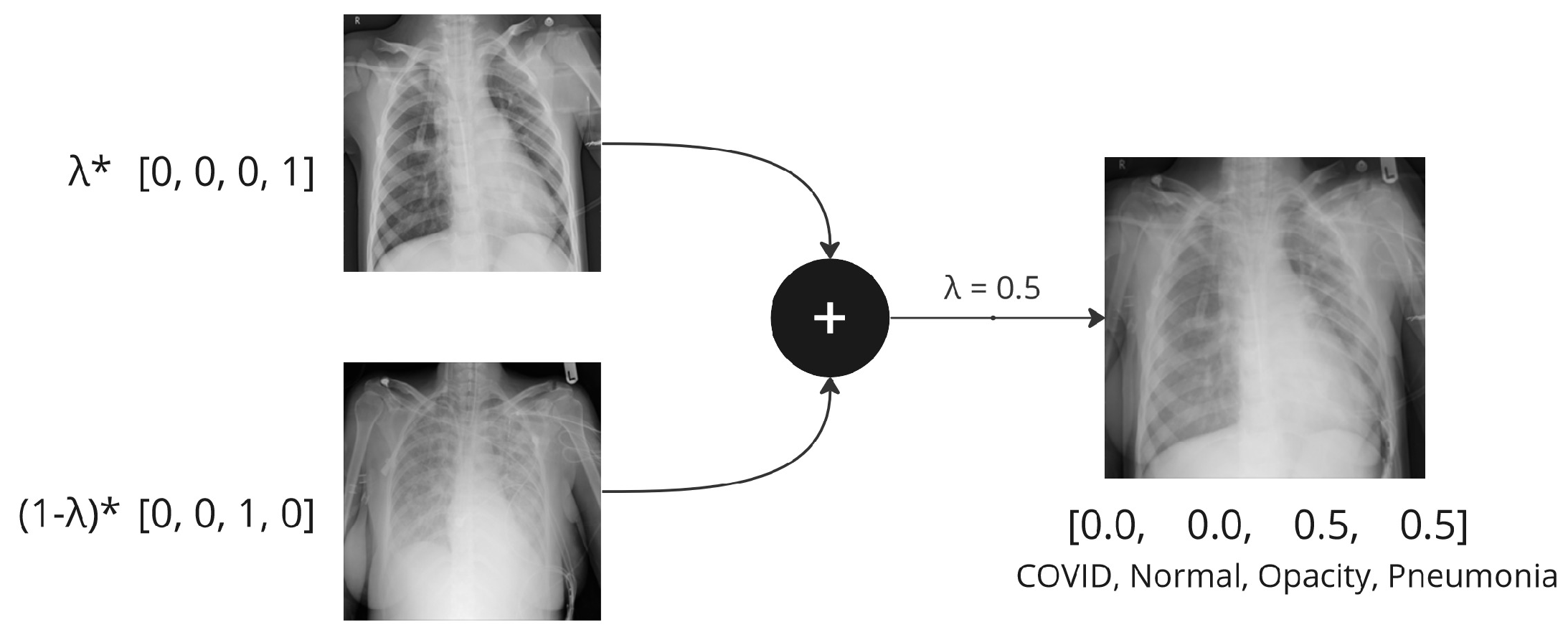

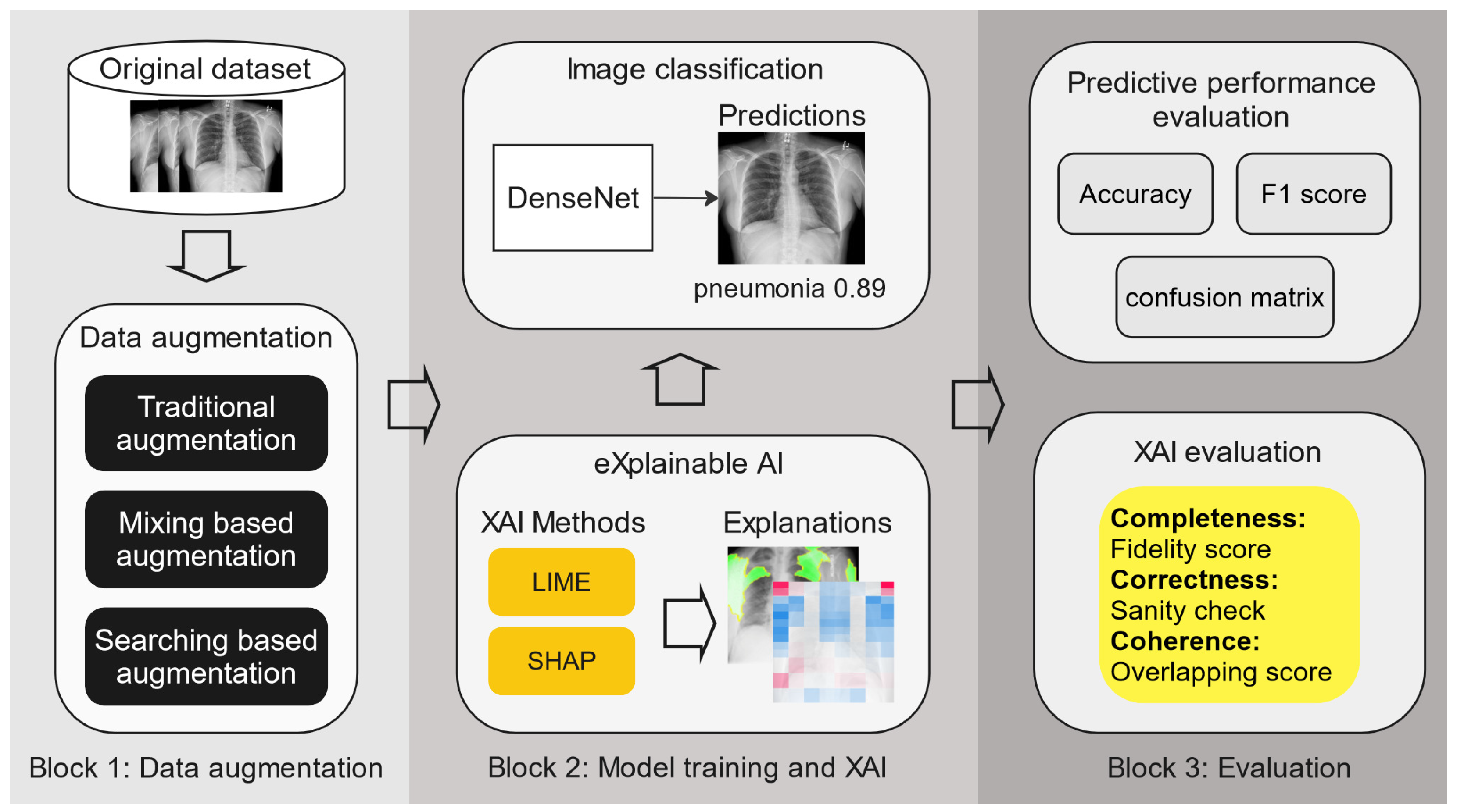
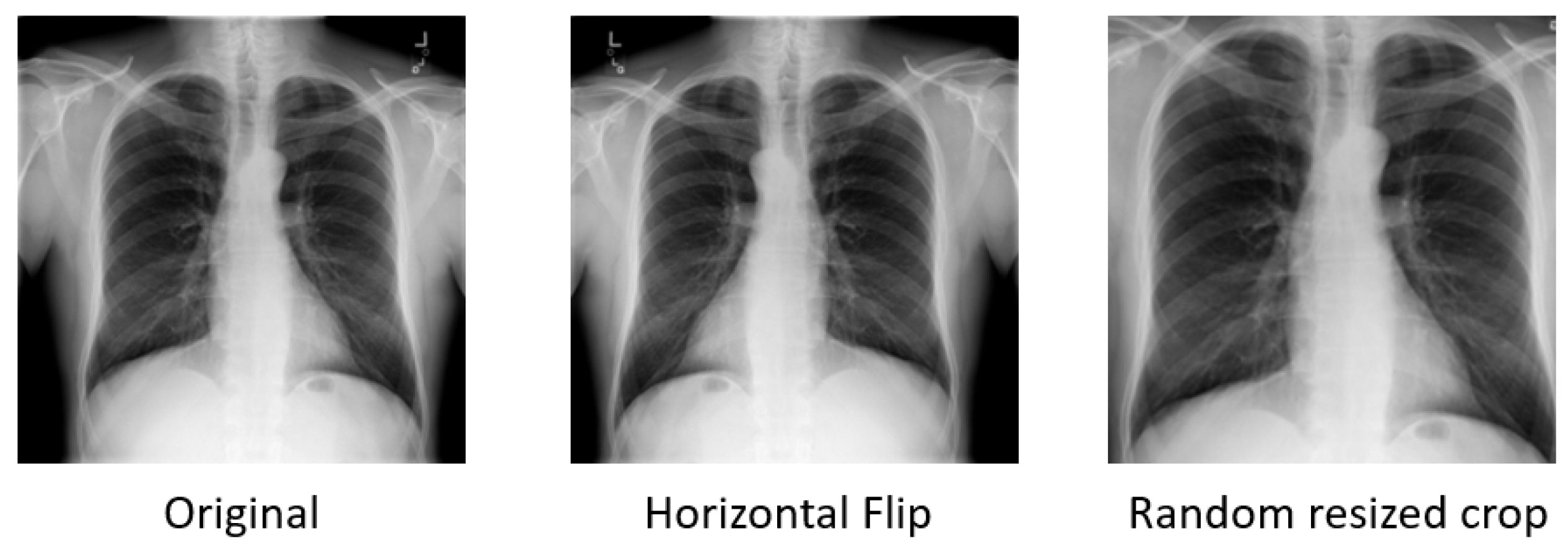
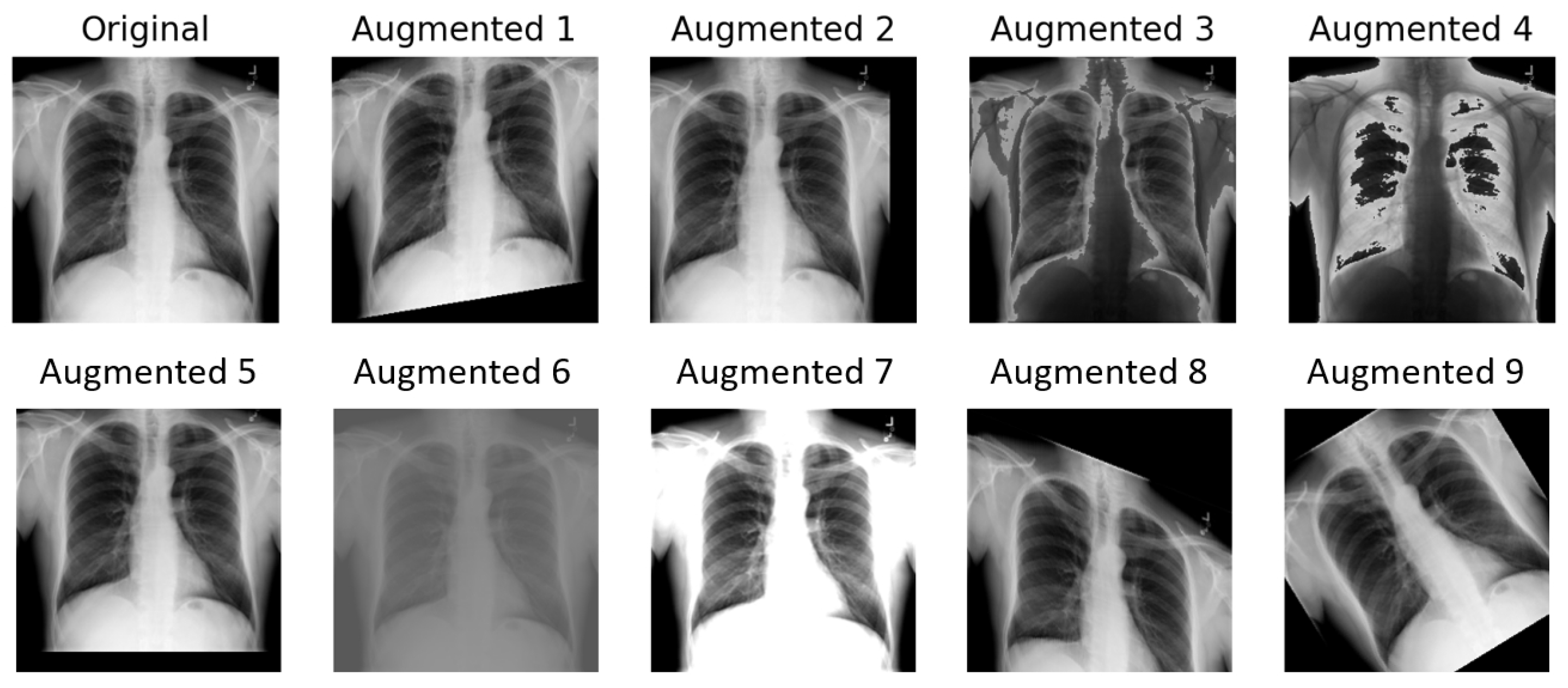
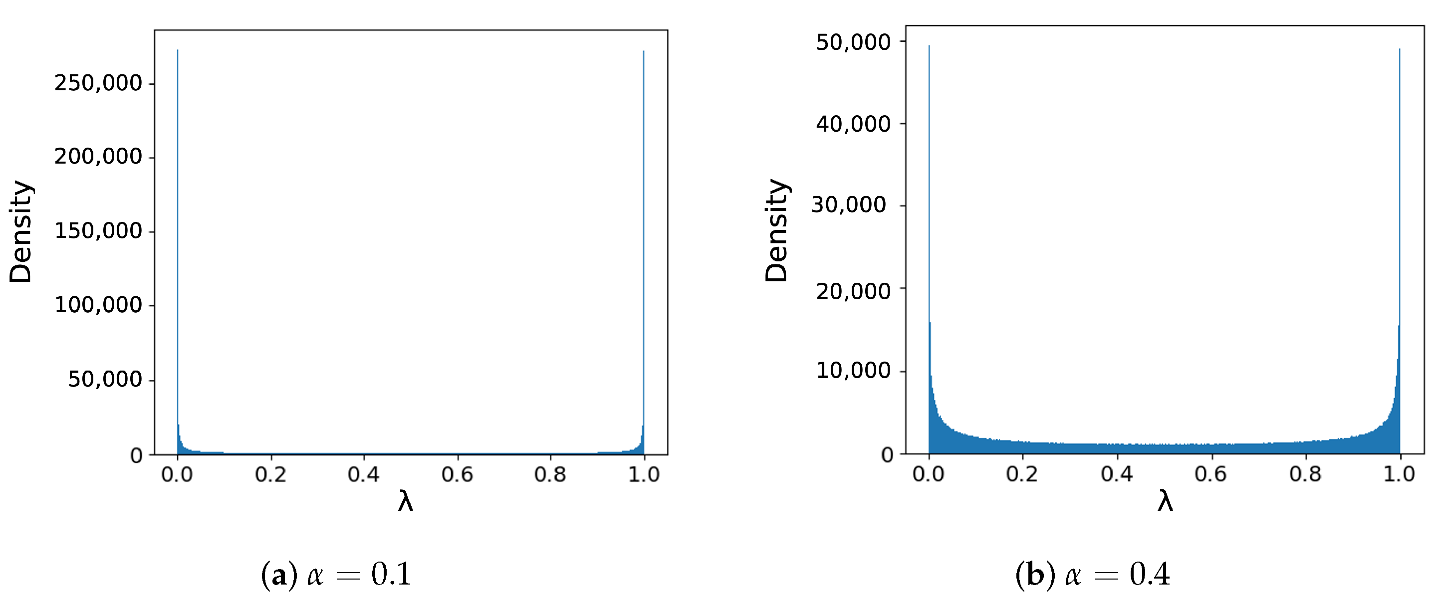
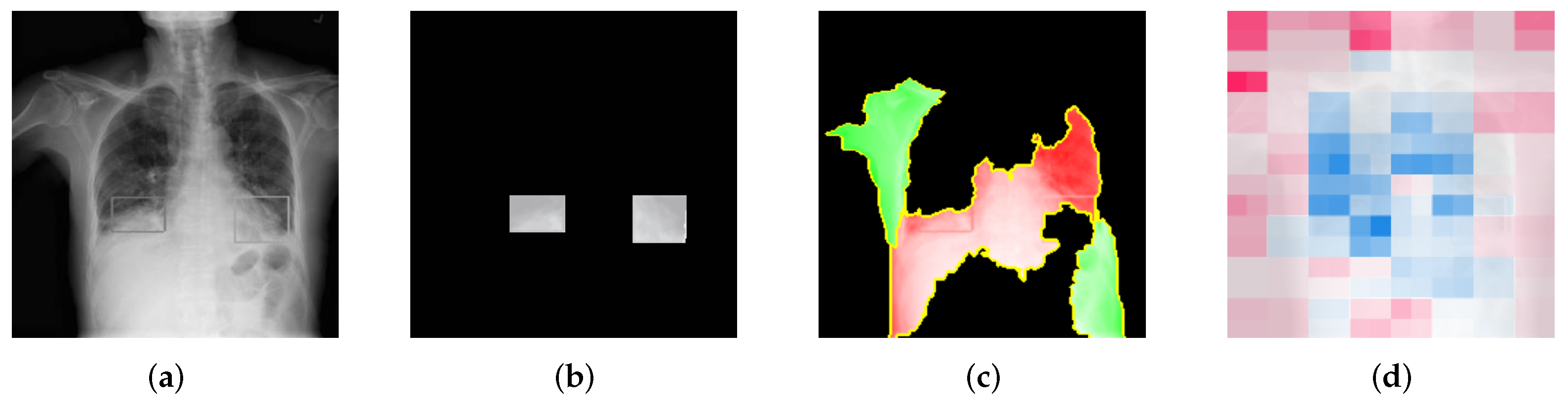
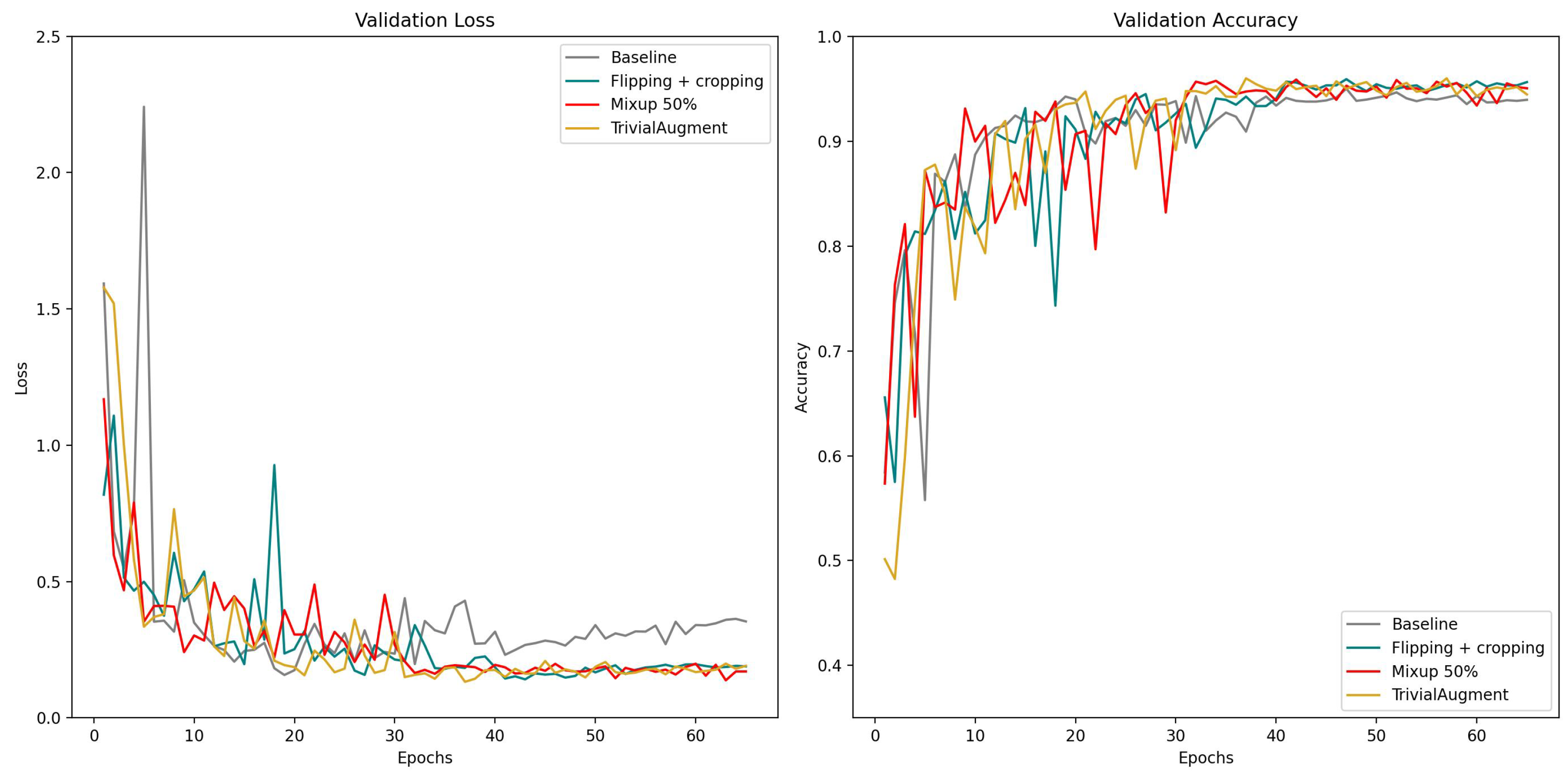
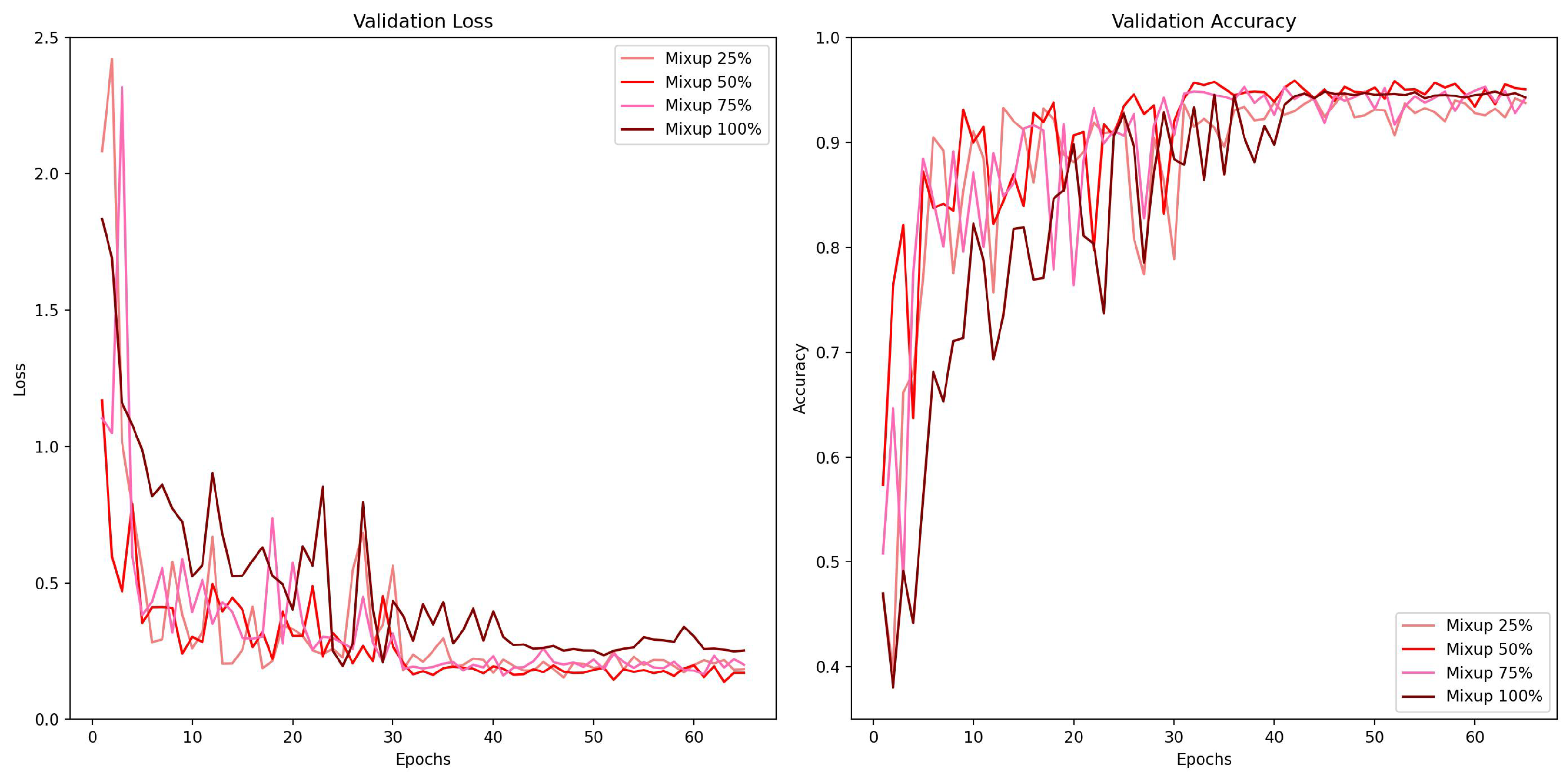
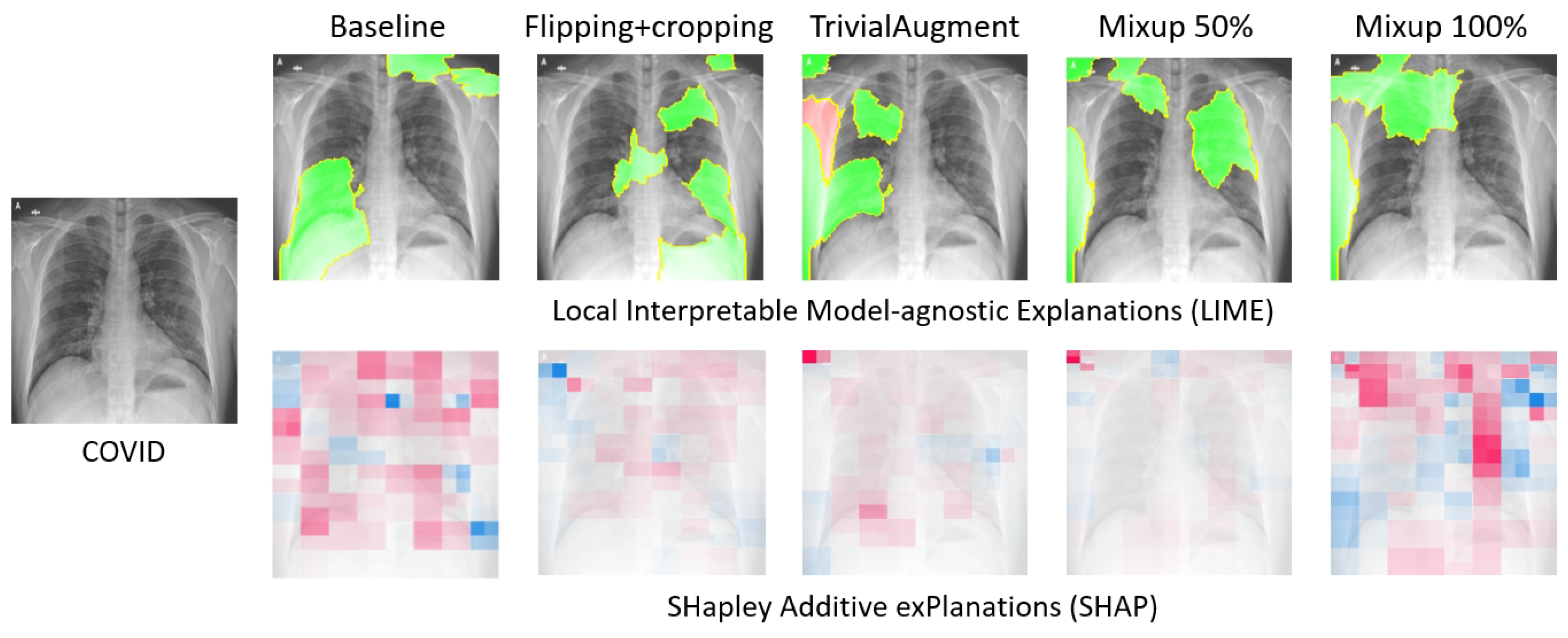

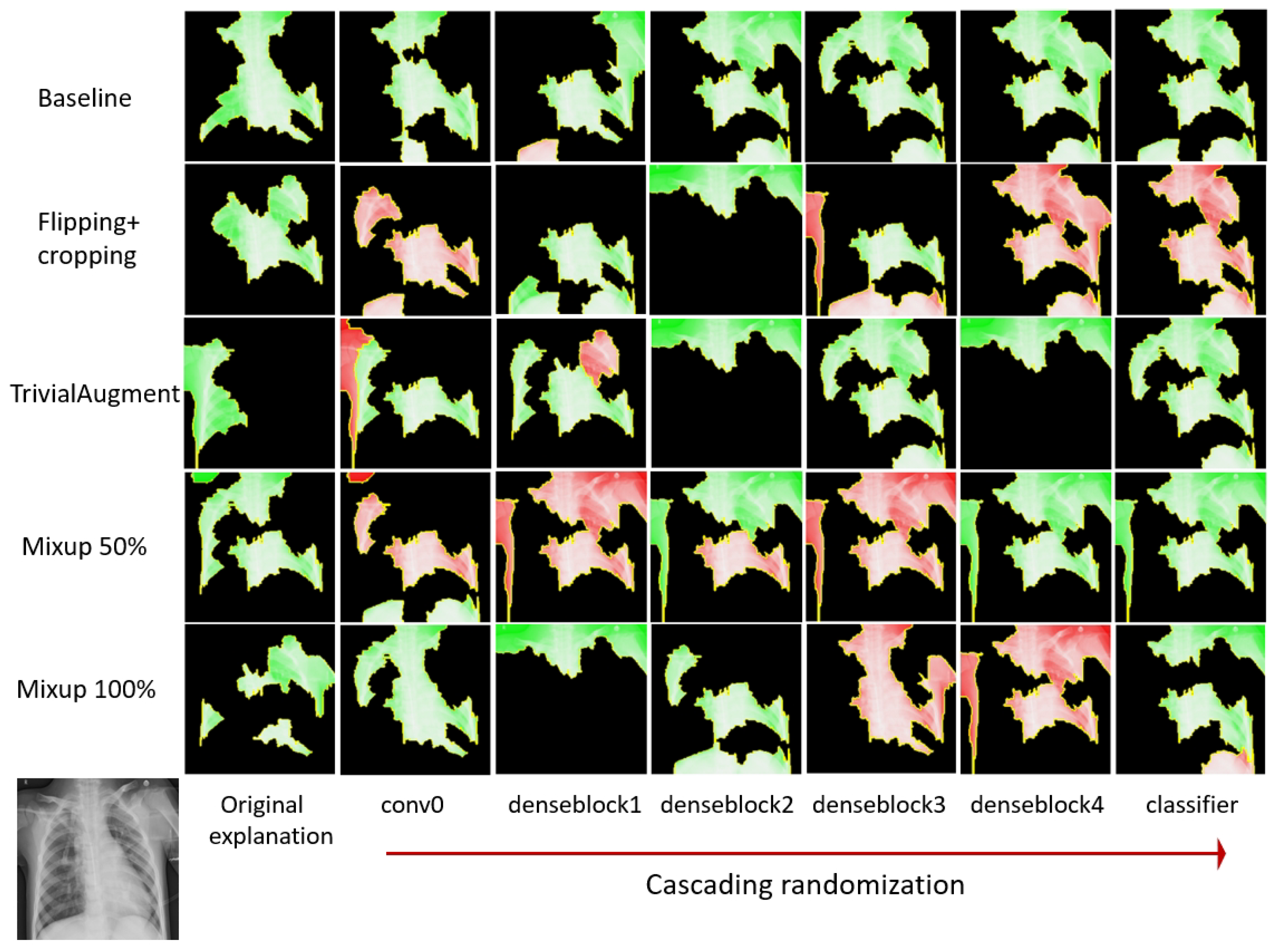

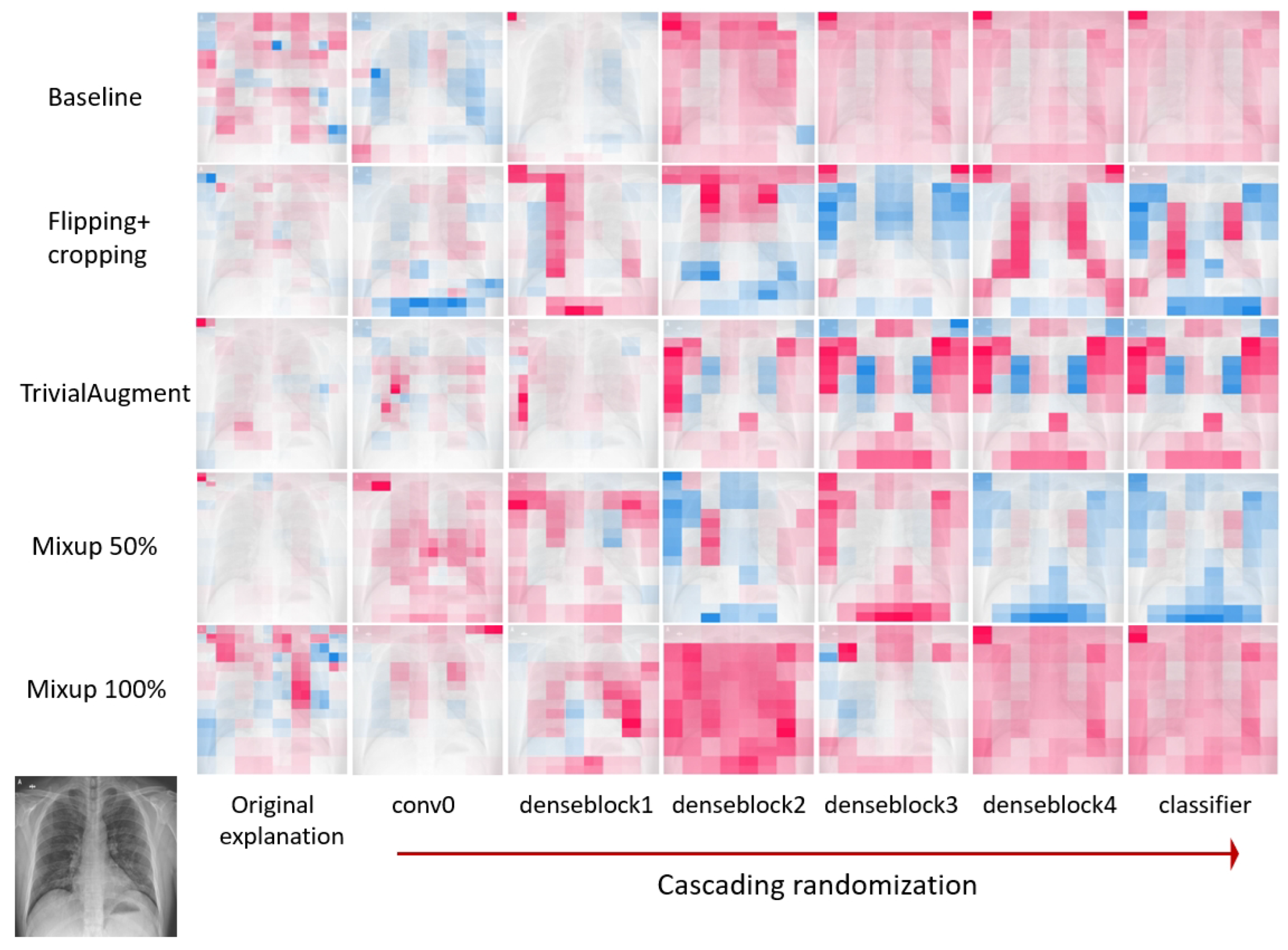
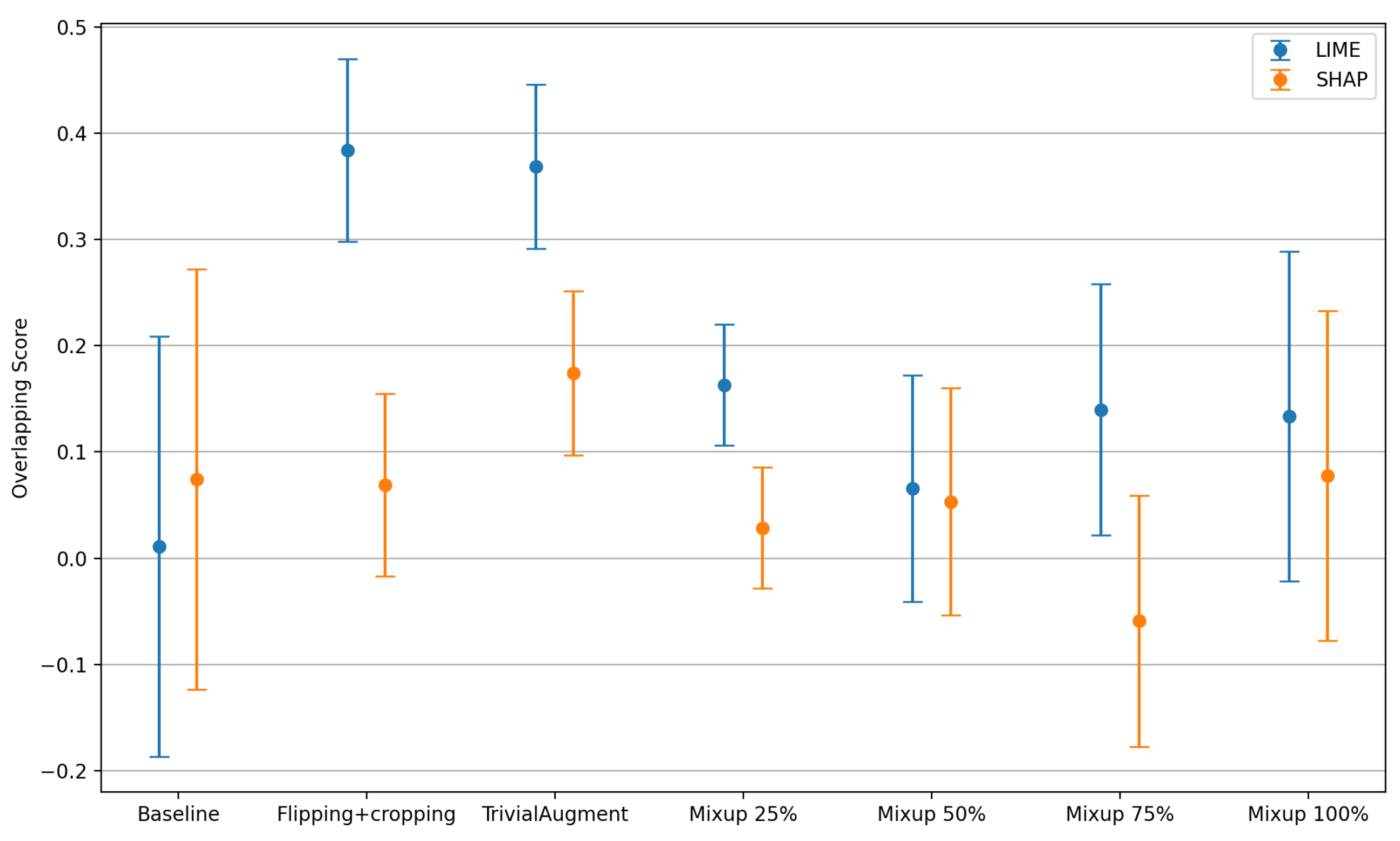
