Article

Exploring Downscaling in High-Dimensional Lorenz Models Using the Transformer Decoder

Department of Mathematics and Statistics, San Diego State University, 5500 Campanile Drive, San Diego, CA 92182, USA
Mach. Learn. Knowl. Extr. 2024, 6(4), 2161-2182; https://doi.org/10.3390/make6040107
Submission received: 5 July 2024 / Revised: 9 September 2024 / Accepted: 23 September 2024 / Published: 25 September 2024
(This article belongs to the Topic Big Data Intelligence: Methodologies and Applications)

Abstract

:
This paper investigates the feasibility of downscaling within high-dimensional Lorenz models through the use of machine learning (ML) techniques. This study integrates atmospheric sciences, nonlinear dynamics, and machine learning, focusing on using large-scale atmospheric data to predict small-scale phenomena through ML-based empirical models. The high-dimensional generalized Lorenz model (GLM) was utilized to generate chaotic data across multiple scales, which was subsequently used to train three types of machine learning models: a linear regression model, a feedforward neural network (FFNN)-based model, and a transformer-based model. The linear regression model uses large-scale variables to predict small-scale variables, serving as a foundational approach. The FFNN and transformer-based models add complexity, incorporating multiple hidden layers and self-attention mechanisms, respectively, to enhance prediction accuracy. All three models demonstrated robust performance, with correlation coefficients between the predicted and actual small-scale variables exceeding 0.9. Notably, the transformer-based model, which yielded better results than the others, exhibited strong performance in both control and parallel runs, where sensitive dependence on initial conditions (SDIC) occurs during the validation period. This study highlights several key findings and areas for future research: (1) a set of large-scale variables, analogous to multivariate analysis, which retain memory of their connections to smaller scales, can be effectively leveraged by trained empirical models to estimate irregular, chaotic small-scale variables; (2) modern machine learning techniques, such as FFNN and transformer models, are effective in capturing these downscaling processes; and (3) future research could explore both downscaling and upscaling processes within a triple-scale system (e.g., large-scale tropical waves, medium-scale hurricanes, and small-scale convection processes) to enhance the prediction of multiscale weather and climate systems.

1. Introduction

Downscaling techniques have been utilized to estimate local, small-scale features of weather and climate systems from global, large-scale patterns. For instance, global weather or climate models with coarser resolutions of 50–100 km are used to provide data for driving limited-area models, also known as regional models, at finer resolutions of a few kilometers (Wilby and Wigley 1997 [1]; Castro et al., 2005 [2]; Maraun et al., 2010 [3]; Pielke and Wilby 2012 [4]). This technique makes it computationally feasible to obtain detailed information without running global models at very high resolutions. A common method involves using the outputs of global models at coarser resolutions as initial and lateral boundary conditions for regional models, thereby deriving detailed features at finer resolutions. A similar approach was applied to a regional spectral model driven by a global spectral model (Juang and Kanamitsu 1994 [5]; von Storch et al., 2020 [6]). In this case, weather systems resolved by high wavenumber modes within the regional model are governed by detailed physics and additionally driven by large-scale weather systems at low wavenumbers from the global model. However, due to inherent limitations within this technique, the detailed fine-scale processes obtained from the regional model cannot provide feedback to the coarse-scale processes within the global model. Thus, it is required to have one or more approaches to examine the idea of downscaling.
An explicit or implicit scientific foundation for the downscaling technique relies on establishing a certain physical and statistical relationship between fine-scale and coarse-scale variables. In this study, I propose an approach to construct an empirical model that establishes a statistical relationship between large-scale and small-scale variables, which I then use to estimate small-scale variables from large-scale data. To achieve my objectives, I utilize high-dimensional Lorenz models to generate small- and large-scale variables and construct empirical models using transformer technology, a state-of-the-art machine learning method employed in current large language models and AI-powered weather prediction systems (Pathak et al., 2022. [7]; Bi et al., 2023 [8]; Bonev et al., 2023 [9]; Chen, Han, et al., 2023 [10]; Chen, Zhong et al., 2023 [11]; Nguyen. et al., 2023 [12]; Selz and Craig 2023 [13]; Watt-Meyer et al., 2023 [14]; Bouallègue et al., 2024 [15]; Li et al., 2024 [16]).
Although linear regression methods were commonly used for predictions in the 1950s (Wiener 1956 [17]), researchers also began to produce realistic predictions using physics-based partial differential equations (PDEs, Charney et al., 1950 [18]). In 1960, at the first numerical weather prediction conference held in Tokyo, Japan, Lorenz presented an analysis of irregular solutions from a nonlinear model, attributing the failure of linear regression methods to the linear assumption (Lorenz 1962 [19]). In the ensuing years, Lorenz continued to explore simpler nonlinear models to highlight the difficulties in obtaining long-term predictions for irregular solutions (Lorenz 1993 [20]; see a review by Shen et al., 2023 [21]). In 1963, Lorenz published a seminal article titled “Deterministic Nonperiodic Flow”, where he simplified Saltzman’s seven-variable model into a three-variable system (Saltzman 1962 [22]; Lorenz 1963 [23], 1993 [20]; Lakshmivarahan et al., 2017 [24]; Lewis and Lakshmivarahan 2022 [25]). This groundbreaking work, along with other studies, later laid the foundation for chaos theory, regarded as one of the three major scientific discoveries of the 20th century (Gleick 1987 [26]), including relativity and quantum mechanics. The feature associated with an irregular nonperiodic solution is now known as chaos (Li and Yorke 1975 [27]).
Over the past five decades, the Lorenz 1963 model has been extensively studied in various fields, including physics, applied mathematics, Earth science, economics, ecology, etc. (Gleick 1987 [26]; Lorenz 1993 [20]; Shen et al., 2023 [21]). Notably, the development of high-dimensional Lorenz models (Curry 1978 [28]; Curry et al., 1984 [29]; Howard and Krishnamurti 1986 [30]; Hermiz et al., 1995 [31]; Thiffeault and Horton 1996 [32]; Musielak et al., 2005 [33]; Roy and Musielak 2007a, b, c [34,35,36]; Moon et al., 2017 [37]) is particularly relevant to this research. To understand the impact of fine-scale features on predictability within high-resolution global weather and climate models (Shen et al., 2010, 2011 [38,39]), the author has developed a series of high-dimensional Lorenz models that incrementally incorporate higher wavenumber modes, resulting in the generalized Lorenz model (Shen 2014, 2016,2019a b [40,41,42,43]). The generalized Lorenz model includes the following characteristics: (1) an odd number of state variables, five or more, (2) the presence of various attractors (point, chaotic, and periodic), (3) coexisting attractors, (4) accumulated negative feedback, (5) a hierarchical dependence on different spatial scales, and (6) energy conservation in the absence of dissipation. The sixth feature ensures the mathematical and physical consistency between the original Rayleigh–Bénard convection equation and the Lorenz models. Derivations from the Rayleigh–Bénard equation do not introduce additional forcing terms into the generalized Lorenz model, regardless of the number of wave modes used. The fifth feature, hierarchical scale dependence, which may provide a foundation for downscaling, is explored below.
For this study, I utilize five- and seven-dimensional Lorenz models, which are simplified versions of the generalized Lorenz models previously examined by the author and other researchers (Shen 2016 [41]; Felicio and Rech 2017 [44]; Faghih-Naini and Shen 2018 [45]; Reyes and Shen 2019 [46]; Cui and Shen 2021 [47]). These two models were employed to generate chaotic data across various scales, including primary, secondary, and tertiary scales. Then, transformer technology and other relevant machine learning methods were applied to develop empirical models that establish a statistical relationship, presumably a nonlinear one, among the various scale variables and explore downscaling.
Currently, four major types of neural networks include (1) multilayer perceptrons (MLP) or feedforward neural networks (FFNN; Rosenblatt 1958 [48]; Rumelhart et al., 1986 [49]); (2) convolutional neural networks (CNN; LeCun et al., 1998 [50]; Krizhevsky et al., 2012 [51]); (3) recurrent neural networks (RNN) (Elman 1990 [52]; Hochreiter and Schmidhuber 1997 [53]; Atienza 2020 [54]; Theodoridis 2020 [55]); and (4) transformers (Vaswani et al., 2017 [56]; Raschka et al., 2022 [57]). Since MLP and transformer technology are used in this study, both architectures are briefly introduced. The MLP architecture emerged in the 1960s and gained popularity in the 1980s, providing the foundation for modern neural network designs. A typical MLP architecture consists of at least three fully connected layers: input, hidden, and output layers. It processes data in a feedforward manner from the input to the hidden and output layers. In this architecture, the output of each layer becomes the input for the next layer. Initially, a linear transformation is performed on the input data in all layers, followed by the application of an activation function on the transformed data, except in the output layer.
The transformer architecture was first introduced in the paper “Attention is All You Need” by Vaswani et al. (2017). This architecture quickly became the state-of-the-art in natural language processing and other sequential tasks, receiving unprecedented attention following the release of the AI models (e.g., BERT, DALL-E, GTP-3; Bommasani 2022 [58]) and large language model ChatGPT 3.5 during the winter of 2022 (OpenAI 2023 [59]). The transformer architecture introduces the self-attention mechanism, which captures relationships within sequences. By avoiding the recursive computation commonly used in RNNs, transformer technology can process sequences in parallel, enhancing both efficiency and scalability. These innovative features enable large language models and AI-powered weather prediction systems to handle increased model complexity (e.g., a large number of parameters) and process massive volumes of data, thereby improving accuracy. Due to the remarkable capabilities and broad applications of recent transformer-based AI models (Devlin et al., 2019 [60]; Raffel et al., 2019 [61]; Radford et al., 2019 [62]; Yin et al., 2020 [63]; Chen et al., 2020 [64]; Rives et al., 2021 [65]), Bommasani and over a hundred collaborators introduced the term “foundation models”. This term reflects the ongoing, yet significant development status of these AI models (Bommasani et al., 2022 [58]). They argue that the notable achievements of these recent AI models stem from their “scale”, which is facilitated by three key advancements: (1) enhanced computer hardware capable of fast, parallel computing; (2) the evolution of transformer technology, which optimizes this parallelism and hardware utilization; and (3) the availability of extensive training datasets.
Given that the self-attention mechanism can potentially capture global dependencies within long sequences and its parallel processing capabilities, I chose transformer technology as an initial approach for demonstrating downscaling within chaotic Lorenz models. My initial goal is to develop a transformer-based model that utilizes a set of large-scale variables to forecast the temporal evolution of smaller-scale variables.
This study is organized as follows. Section 2 provides a brief introduction to the generalized Lorenz model used to generate chaotic data across multiple scales, including primary-, secondary-, and tertiary-scale variables. I then outline the architecture of the empirical models designed to establish the statistical relationship between primary-scale and secondary-scale variables, utilizing linear regression, FFNN, and transformer technology. Section 3 present the technical detail and performance of the empirical models, highlighting correlations between the true and predicted secondary-scale variables. Section 4 discusses future studies, which will involve examining both downscaling and upscaling processes, implementing the vision transformer (ViT; Dosovitskiy et al., 2020 [66]) to analyze temporal and spatial data, and integrating the core system into an AI-powered weather model to explore predictability horizons. Section 5 offers concluding remarks.

2. Materials and Methods

2.1. A Generalized Lorenz Model

By rederiving the Lorenz 1963 model and extending the nonlinear feedback loop within the 1693 model, Shen (2019a) [42] developed the following generalized Lorenz model (GLM):
d X d t = σ Y σ X ,    
d Y d t = X Z + r X Y ,
d Z d t = X Y X Y 1 b Z ,
d Y j d t = j X Z j 1 j + 1 X Z j d j 1 Y j , j Z : j 1 , N        
d Z j d t = j + 1 X Y j j + 1 X Y j + 1 β j Z j ,        
N = M 3 2 ;   d j 1 = 2 j + 1 2 + a 2 1 + a 2 ; β j = j + 1 2 b ; b = 4 / 1 + a 2 .      
Here, t is dimensionless time. While X , Y j ,   a n d   Z j represent time varying state variables, the remaining terms are time-independent parameters. The integers j, M, and N are specific to high-dimensional Lorenz models. For each of the above terms, please see the details provided in Shen (2019a) [42] and Shen et al. (2021) [67].
Like the classical Lorenz model, the GLM also originates from the Rayleigh–Bénard convection equation. However, the applicability of Lorenz models to real-world issues has been emphasized through establishing a mathematical link between the classical Lorenz model and the Pedlosky model, which itself is derived from a two-layer quasi-geostrophic system (Pedlosky 1971 [68]; Shen et al., 2023 [21]). Furthermore, the extension of the nonlinear feedback loop is based on the nonlinear advection of temperature, a common physical process in both weather and climate systems. Given an integer value of j, Equations (4) and (5) describe a pair of ODEs that govern the evolution of smaller-scale variables Y j and Z j . These ODEs introduce linear dissipative terms (e.g., d j 1 Y j and β j Z j ) as well as nonlinear terms. As previously demonstrated, nonlinear terms act as “coupling terms”, providing feedback to larger scale variables (e.g., Equations (1)–(3)), and introduce an additional incommensurate frequency (e.g., Figure 10 of Faghih-Naini and Shen 2018 [45]; Figure 11 of Shen 2019a [42]).
In this research, I implement ML-based empirical models based on outputs from the GLM with M = 5 and M = 7, referred to as the five- and seven-dimensional Lorenz models (5DLM and 7DLM, Shen 2014, 2016 [40,41]), respectively. High-dimensional Lorenz models that incorporate even numbers of modes (e.g., six or eight modes) are also utilized (see the review by Shen et al., 2023 [21]) and may offer additional support to the results obtained using the 5DLM and 7DLM. As outlined in Shen (2014, 2019a [40,42]), each time-varying state variable signifies the amplitude of the Fourier mode corresponding to a specific pair of horizontal and vertical wavenumbers.
Shen (2016) [41] classified X , Y ,   a n d   Z as primary-scale variables, X 1 , Y 1 ,   a n d   Z 1 as secondary-scale variables, and X 2 , Y 2 ,   a n d   Z 2 as tertiary-scale variables. The terms primary-scale “variables” and “modes” are used interchangeably throughout this study. X 1 and X 2 , present in models with even numbers (e.g., 6D and 8D Lorenz models), are excluded to simplify the discussion in this study. Both the 5DLM and 7DLM produce primary- and secondary-scale variables, while the 7DLM additionally generates tertiary-scale variables. This study seeks to create ML-based empirical models that utilize primary-scale variables to estimate the values of secondary-scale variables. Comparing models trained by various data from the 5DLM and 7DLM can implicitly reveal the impact of tertiary-scale variables.
In my generalized Lorenz model, higher dimensional systems necessitate larger values of the heating parameter (r) to produce chaotic data (e.g., Table 2 of Shen 2019b). Consequently, I use r = 50 and r = 120 for the 5DLM and 7DLM, respectively, in order to generate chaotic data while other parameters, including σ = 10 ,   a 2 = 1 / 2 , and b = 8 / 3 , are kept constant. The selection of parameters a and b aligns with previous studies, resulting in d 0 = 19 / 3 and d 1 = 17 . All state variables are initiated at a value of one in the control runs. The property of sensitive dependence on initial conditions is demonstrated by comparing the control and parallel runs, which only differ by small initial perturbations in variable Y (e.g., ϵ = 10 5 ). All simulations were conducted using a time step of 0.001 and the Runge–Kutta–Fehlberg (RKF45) scheme provided by the SciPy package version 1.13.0 for Python (Virtanen et al., 2020 [69]). During the time interval between 0 and 20 (or 25) for the 5DLM (or 7DLM), there are 20,000 (or 25,000) data points for each variable.

2.2. Chaotic Data Preparation

One of the most intriguing features of chaotic solutions is their sensitive dependence on initial conditions (SDIC), also known as the butterfly effect or, more specifically, the first kind of butterfly effect (Shen et al., 2022 [70]; Pielke Sr. et al., 2024 [71]). This feature and its implications for finite predictability are discussed below.
Using the GLM, each state variable can be represented as a time series. To describe the evolution of the solution using multiple state variables, one can imagine a solution corresponding to a specific set of initial conditions, e.g., (X, Y, Z, Y1, Z1) = (1, 1, 1, 1, 1) for the control run, representing a trajectory moving through space over time. When this space is constructed using state variables, it is called a phase space. A solution to a different set of initial conditions, e.g., (X, Y, Z, Y1, Z1) = (1, 1+ ϵ , 1, 1, 1) and ϵ = 10 5 for the parallel run, represents a different trajectory. As shown in Figure 1, the two initially nearby trajectories, meaning two solutions with a tiny difference in their initial conditions, exhibit similar paths during the initial stage but diverge significantly later. These two distinct features are referred to as continuous dependence on initial conditions (CDIC) and SDIC, respectively.
While CDIC is necessary for the existence of solutions, SDIC is a crucial factor that defines a chaotic system. If one views the solution of the control run as the true solution and the solution of the parallel run as the predicted solution, the occurrence of SDIC between the two solutions renders the parallel run unreliable. Thus, the predictability horizon is defined as the interval between the initial time and the onset of SDIC. Since any chaotic system exhibits SDIC, its predictability is finite (Lighthill 1986 [72]).
This study focuses on downscaling, specifically whether smaller scale variables can be estimated using large-scale variables. While this study does not attempt to predict the onset of chaos, it aims to understand whether an empirical model trained using data from the control run within the CDIC time interval can estimate small-scale variables after the onset of SDIC for both the control and parallel runs.
One of the goals of this study is to introduce ML-based methodologies to researchers who have prior experience with linear regression models. To this end, I have chosen methods to develop empirical models that gradually enhance both complexity and flexibility. The upcoming section will explore the architecture and performance of each ML-based empirical model.

3. ML-Based Empirical Models and Their Performance

To achieve my goal, Figure 2 presents a flowchart for processing data, which includes an input component on the left, an ML-based empirical model in the middle, and an output component on the right. I utilized the GLM to generate data for training various ML-based empirical models, including the linear regression model, the feedforward neural network (FFNN)-based model, and the transformer-based model. All ML-based models are trained and validated using the same dataset from the control run of the 5D or 7D Lorenz Model (5DLM or 7DLM), where primary scale modes (X, Y, Z) serve as inputs and secondary scale modes (Y1, Z1) as outputs. For the 5DLM, the simulation was conducted for twenty units, providing training data for the first fifteen time units and validation data for the last five time units. For the 7DLM, it generates training data for twenty time units and validation data for the subsequent five time units. The selection of total integration, training, and validation periods is based on my extensive experience with Lorenz model simulations (e.g., Shen 2014, 2016, 2019a, b, 2023 [40,41,42,43,73]). I anticipate that findings are not highly sensitive to these periods, provided that the training duration is sufficiently long, approximately 10 time units or more.

3.1. Linear Regression Model

Below, to illustrate the key point, a linear regression model is first discussed. Since three primary scale variables are used as inputs, the secondary scale mode Y1 can be estimated using the following expression:
Y 1 ^ = β o + β 1 X + β 2 Y + β 3 Z .  
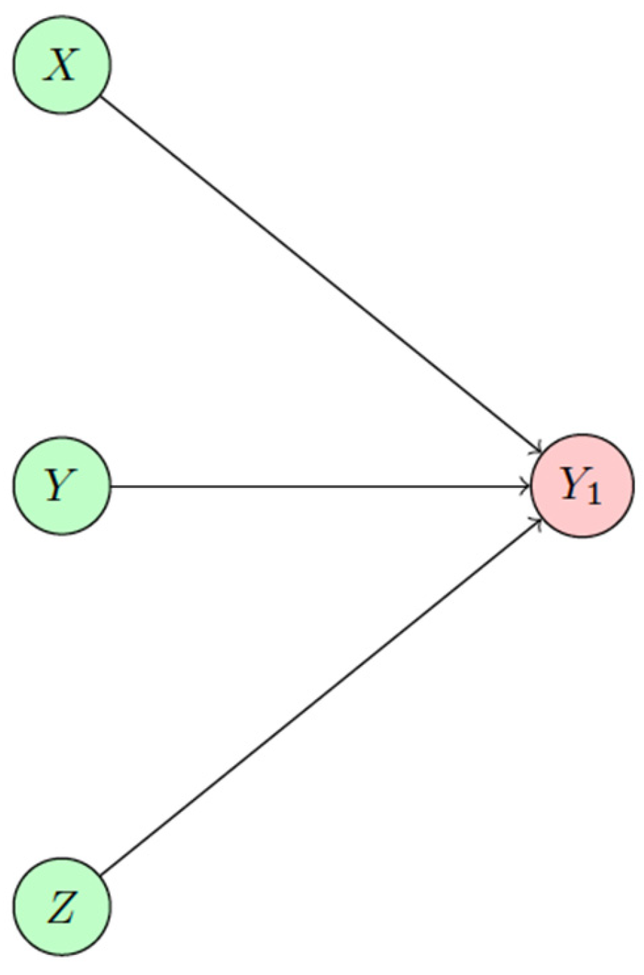
Here the variable Y 1 ^ with a hat represents an estimated value of Y1. Figure 3 illustrates the relationship between the input and output variables. Each arrow corresponds to a coefficient β j ,   j = 1, 2, 3, also known as weights. β 0 presents a bias term. By optimizing the mean squared error, i = 1 N Y 1 Y 1 ^ 2 / N , for N training data, all parameters β j can be determined. Consequently, Equation (7), along with new data during the validation period, can be used to estimate Y1. Thanks to the rapid advancement of modern computing technology, these procedures can be efficiently executed using existing packages, such as the Scikit-learn package version 1.5.0 (e.g., Raschka et al., 2022 [57]).
In addition to the linear regression model, Figure 3 also depicts a simple perceptron (SP), which includes an input layer with three variables and an output layer with one variable. Therefore, I utilized the torch.nn module from the recently developed PyTorch package (Raschka et al., 2022 [57]) to implement another empirical model and compared it with the aforementioned linear regression model using the Scikit-learn package for further verification. As shown in Figure 3, an empirical model is constructed using an identity function as the activation function, effectively making it a linear activation function. To efficiently train this empirical model and to allow for slight differences between the two models, I first removed the mean from both input and output variables to obtain perturbations and then normalized these perturbations by their standard deviations. Scaled input and output perturbations were then used to train the model. Consequently, the empirical model estimates a scaled perturbation of Y1. To obtain the total value of Y1, I needed to rescale the predicted perturbations and add back the mean.
Figure 4 presents the results from the two linear models. The first two panels illustrate the predicted results Y1 for the training period, while the last two panels show the estimated Y1 during the validation period. Both empirical models yielded comparable results, with Pearson correlation coefficients close to one for both the training and validation periods. Differences in the predicted amplitudes in panel (d) are associated with the bias term. The models predicted Y1 in good agreement with true Y1 during the training period, while predicted Y1 values exhibited slightly larger errors during the validation period. Correlation coefficients between the predicted and true values of Y1 are 0.92 and 0.91 for the training and validation periods, respectively.

3.2. Feedforward Neural Network (FFNN)

Given that an FFNN-based model is a fundamental component of neural networks and is incorporated as sub-layers within transformer technologies, I present the performance of a simple FFNN-based model for exploring downscaling within the GLM. This model serves as a bridge between the previously mentioned linear models, i.e., the regression and simple perceptron models, and the transformer-based model, which will be discussed further. Figure 5 illustrates the architecture of the FFNN for the empirical model. This model comprises an input layer with three variables, two fully connected hidden layers with 10 units each, and an output layer with two variables. A ReLU activation function is applied to the net input of the first hidden layer, as commonly employed in hidden layers. The choice of two hidden layers with 10 units each was made to introduce diversity in approaches, compared to the linear models and the transformer-based model. While this specific FFNN-based model is used to provide a proof of concept, I observed larger errors when five units per layer were used.
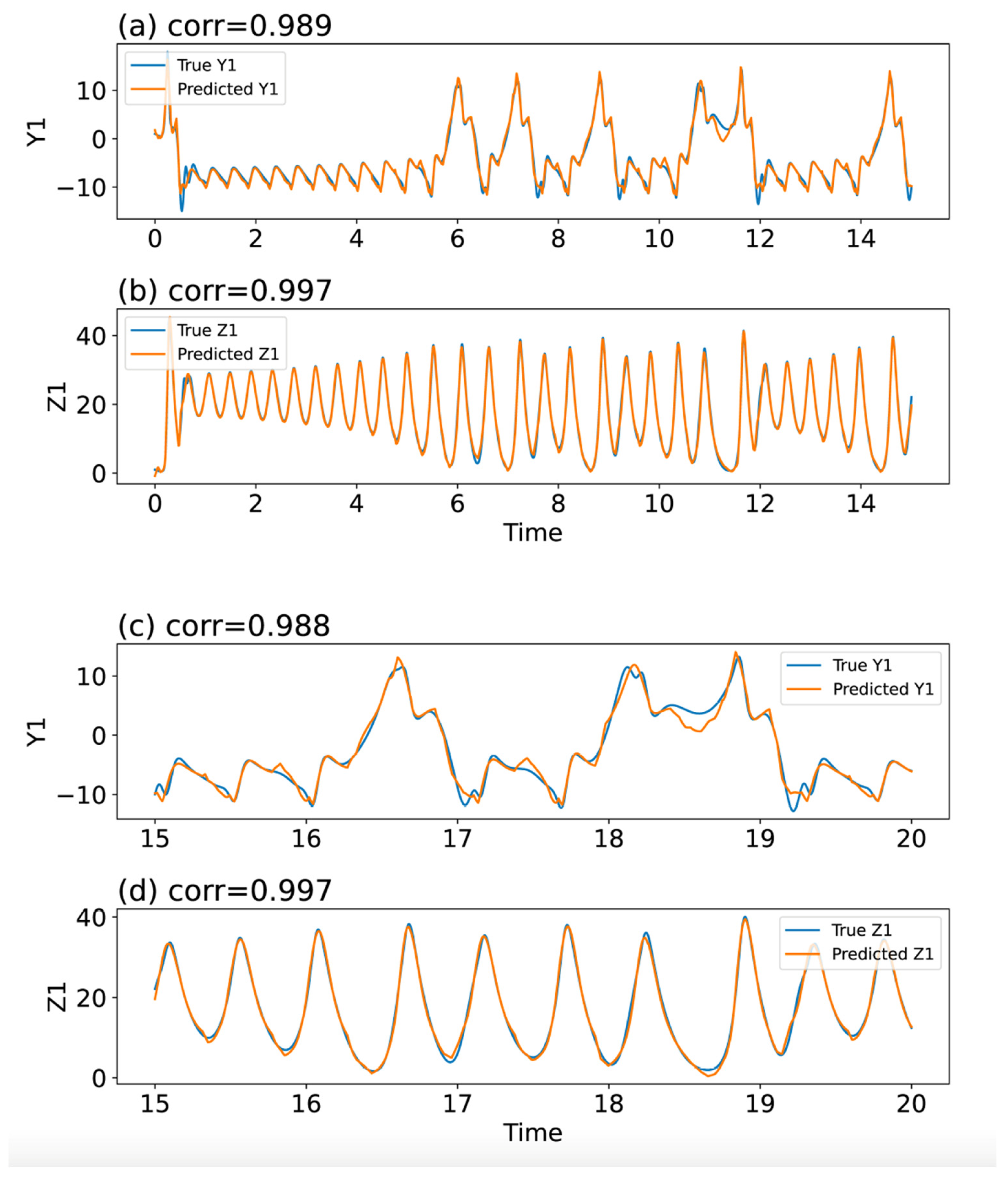
In contrast to the linear models (i.e., the regression and simple perceptron models), the FFNN-based empirical model introduces additional complexity while using the same three input variables but producing two output variables. Figure 6 illustrates the predicted secondary scale variables, Y1 and Z1. It is evident that the results shown in Figure 6a,c provide more accurate predictions for Y1 compared to Figure 4a,c. Specifically, correlation coefficients between the predicted and true values of Y1 are now 0.989 and 0.988 for the training and validation periods, respectively, compared to 0.92 and 0.91 in the linear models. However, the primary purpose of this comparison is to demonstrate the functionality and flexibility of PyTorch in handling more complex features, such as varying numbers of outputs that may represent different physical variables. For example, this model predicts another secondary scale variable Z1, which is also in good agreement with the true variable.

3.3. Transformer Technology

One primary objective of this research is to assess the effectiveness of transformer technology in downscaling and to utilize the insights gained as a foundation for future studies. Figure 7 illustrates the structure of the transformer-based empirical model, which incorporates input and output variables from the GLM. The decoder of the transformer technology is utilized, and the model is implemented using the PyTorch package. The components of the model and their respective functions are detailed as follows:
  • Embedding Layer:
    Converts the input time series (X, Y, Z) into a higher-dimensional space, designated as a hidden dimension of 64 (h_dim = 64).
  • Positional Encoding:
    Adds positional encoding to the embedded input to provide temporal information.
  • Transformer Decoder Layers:
    Positionally encoded input is processed through three consecutive transformer decoder layers.
    Each layer, featuring multi-head attention mechanisms, processes the input and forwards its output to the subsequent layer, as elucidated below.
  • FeedForward Neural Network (FFNN):
    Output from the last transformer decoder layer feeds into a feedforward neural network (i.e., a fully connected layer).
    This layer reduces dimensionality from the hidden dimension to the output dimensions of Y1 and Z1.
  • Output:
    Final output from the fully connected layer represents the predicted values Y1 and Z1.
In the empirical model, the three transformer decoder blocks are essentially identical. Each decoder block consists of the following sublayers:
  • Self-Attention: Enables the model to attend to all positions within the input sequence.
  • Feedforward Network: Processes the output from the self-attention mechanism.
  • Layer Normalization and Residual Connections (He et al., 2015 [74]): Applied within each sublayer to stabilize and enhance the learning process.
Since the model only includes only a decoder, there is no sublayer for cross-attention with encoder outputs.
One of the major features of transformer technology is the self-attention mechanism. This mechanism considers the relationship of each input element with itself and with other elements to generate outputs. Three matrices, known as Q (Query), K (Key), and V (Value), are introduced as learnable parameters. These matrices are used to compute a similarity matrix (i.e., self-attention matrix), which is then used to generate the weighted sum as the output of the decoder sublayer.
When the Q (Query) and K (Key) matrices are projected into smaller subspaces, the self-attention mechanism can be independently applied to each pair of Q and K submatrices. This technique is known as the multi-head attention mechanism. Each head operates on a different subspace, utilizing its own set of weights, which allows the model to simultaneously focus on various aspects of the input sequence. By processing multiple attention heads in parallel, the multi-head attention mechanism captures diverse features and enhances the model’s ability to learn richer representations.
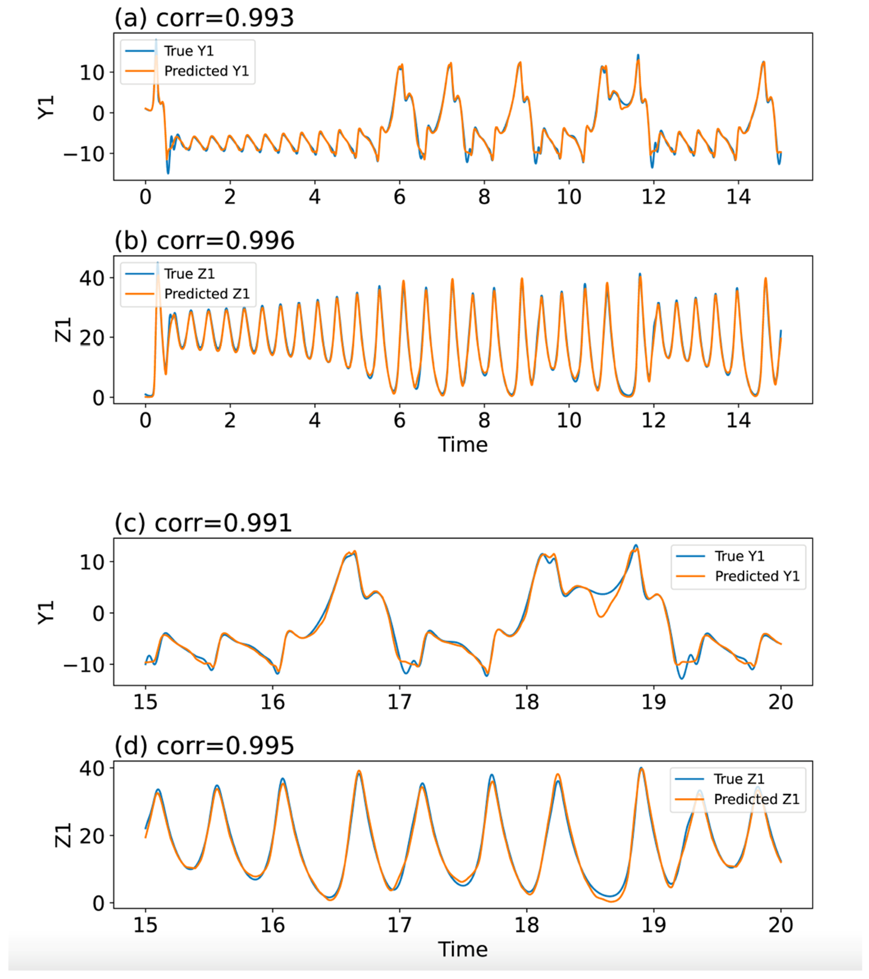
Similar to the first three empirical models, the empirical model described in Figure 7 is trained using GLM data. This model is then applied to predict the secondary scale variables Y1 and Z1. As shown in Figure 8, the transformer-based model improved the accuracy of the estimated results for the variable Y1 compared to the other three empirical models, even though it was not specifically tuned for performance. Correlation coefficients between the predicted and true values of Y1 are now 0.993 and 0.991 for the training and validation periods, respectively, compared to 0.989 and 0.988 in the FFNN-based model. Table 1 provides a comparison of the correlation coefficients, while Table 2 presents the relative root mean squared errors (RMSEs) for the linear regression-, FFNN-, and transformer-based models. However, correlation coefficients for the estimated Z1 are 0.001 or 0.002 lower compared to estimates from the FFNN-based model.
This case provides a proof of concept that the transformer-based model is also capable of revealing downscaling within the GLM. In a future study, the capability of the transformer-based model will be explored through eigenvalue analysis of the Q, K, and V matrices, as well as the eigenvalue analysis of weight matrices in FFNN-based models with linear or nonlinear activation functions.
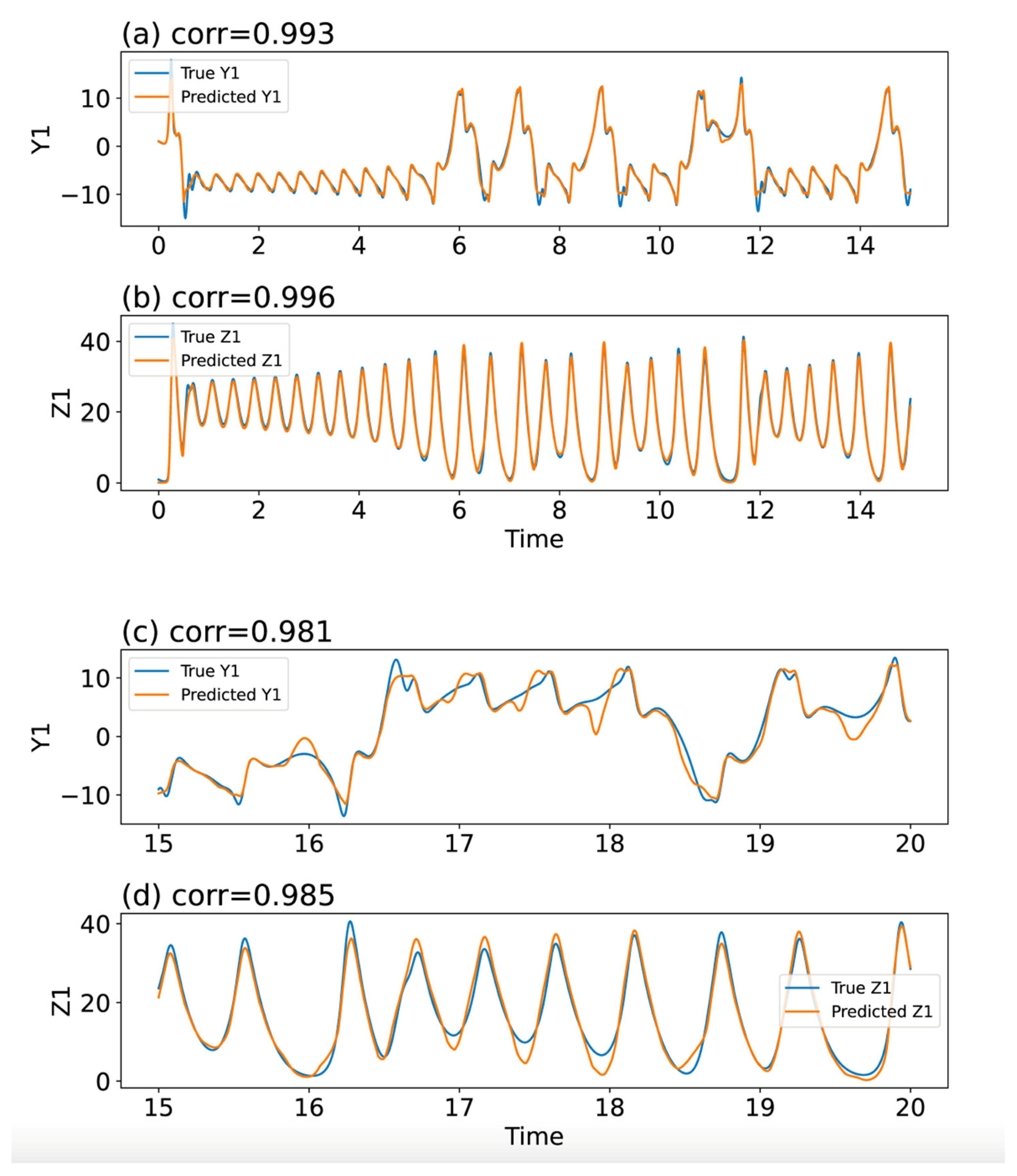
Below, I further validate the performance of the ML-based models in capturing downscaling using a different dataset. It is noteworthy that the 5DLM produces chaotic solutions. As demonstrated by the control and parallel runs in Figure 1, SDIC (i.e., the first kind of butterfly effect) emerges between time = 15 and time = 16. Although all empirical models were initially trained with data from the control run between time = 0 and time = 15, it is intriguing to assess whether these ML-based models can accurately predict the secondary scale variables using data from the parallel run, especially during periods when SDIC occurs post-training. To investigate this, I employ primary scale variables (X, Y, Z) from the parallel run to drive the transformer-based empirical model. The predicted variables Y1 and Z1, as illustrated in Figure 9, are generally well-predicted during both the training and validation phases. In fact, the statistics of predicted Y1 and Z1 are the same over the training period using both the control and parallel run data. However, slightly larger errors in Y1 and Z1 are recorded between time = 17 and time = 18.5 during the validation period, in contrast to the results shown in Figure 8. For the validation periods, the correlation coefficients between the predicted and true values of Y1 (and Z1) are 0.981 (and 0.985) when parallel run data are used, compared to 0.991 (and 0.995) using the control run data. As a result, this case reinforces the time-varying connection of secondary scale variables on the collective influence of primary scale variables.

3.4. Additional Verification Using the 7DLM

While the 5DLM produces two scales of variables—primary and secondary—the 7DLM introduces an additional, smaller scale known as tertiary scale variables, specifically Y2 and Z2. Ideally, this allows for an examination of both the individual and combined impacts of large-scale variables (X, Y, Z) and small-scale variables (Y2, Z2) on the estimates of medium-scale variables (Y1, Z1).
This concept aligns with the triple scale conceptual model proposed by Shen et al. (2013) [75], which analyzed how medium-scale hurricane simulations were influenced by large-scale tropical systems or waves, such as African easterly waves, and the feedback from small-scale flows, such as convection and precipitation. Following this, the 10-year multiscale analysis by Wu and Shen in 2016 [76] suggested that the downscale transfer of energy by intensifying African easterly waves could significantly contribute to hurricane formation, potentially extending the lead time of hurricane predictions. This study supported the 30-day predictability previously reported by Shen et al. (2010) [38] and further discussed by Shen (2019b) [43]. However, the findings of Wu and Shen (2016) [76], compared to the triple scale model, imply that large-scale flows with a memory of feedback from all smaller scales may be used to determine major features at other scales, such as specific hurricanes, particularly when a connection between a specific easterly wave and hurricane is established, whether implicitly or explicitly. Below, this idea is explored using the 7DLM.
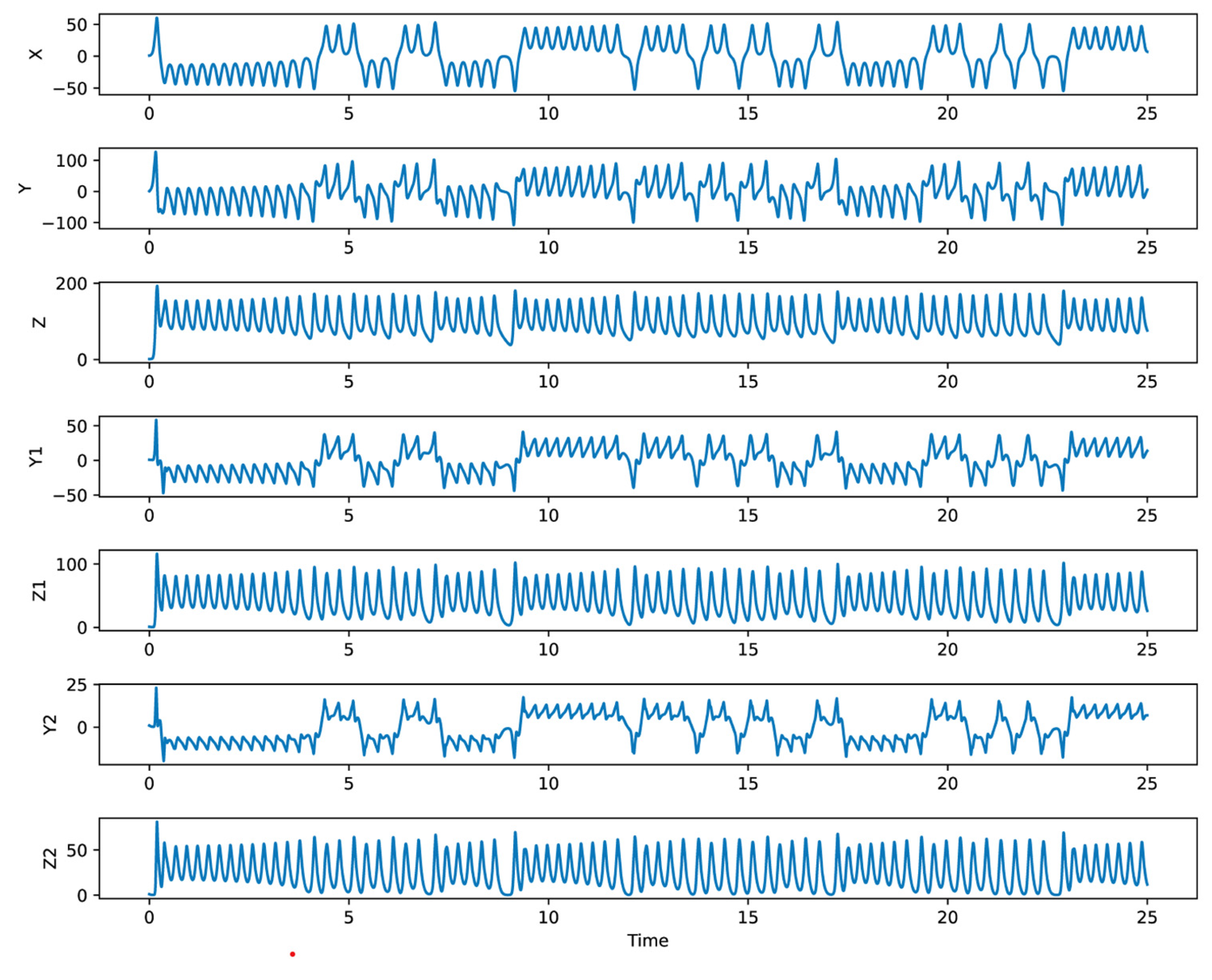
A control run using the 7DLM with r = 120 was conducted over 25 time units to generate both training and validation data. Compared to the 5DLM, the 7DLM requires a higher value of r to produce chaotic solutions due to the negative feedback effects from the tertiary scale variables. This negative feedback is linked to the linear terms with negative coefficients found in Equations (4) and (5), which originate from dissipation terms in the classic Rayleigh–Bénard convection equation. Figure 10 illustrates the solution for all variables in the 7DLM. Key characteristics include irregular oscillations and, for smaller scale variables, reduced amplitudes and increased frequencies; this can be seen in a comparative analysis of the Y, Y1, and Y2 variables as well as the Z, Z1, and Z2 variables.
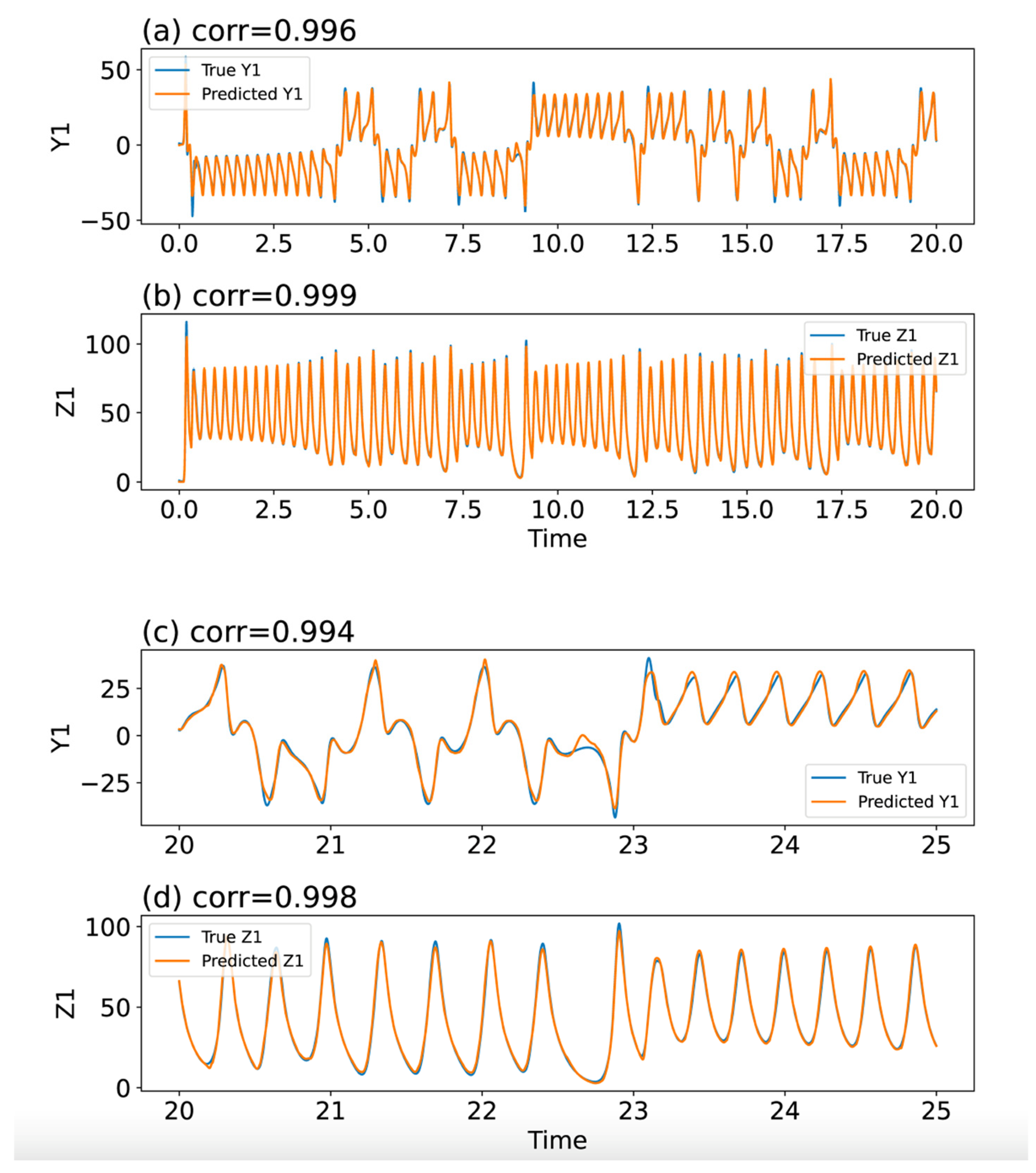
An empirical model, following the same architecture depicted in Figure 7, utilizes solutions from the 7DLM for training and validation. The model uses the first twenty time units of solutions as training data and the following five time units as validation data. Mirroring the approach of the 5DLM-transformer-based model, this new transformer-based model is trained using the primary scale variables as inputs and the secondary scale variables as outputs. The empirical model is subsequently employed to predict the secondary scale variables from the primary scale variables. Figure 11 displays estimated and true values of the Y1 and Z1 variables, showing highly accurate results over both the training and validation periods, even though the new empirical model does not explicitly include the impact of tertiary modes. Interestingly, as shown in Figure 8 and Figure 11, the correlation coefficients between each predicted variable and the corresponding true variable are slightly higher in the 7DLM case than in the 5DLM case. As a result, downscaling capability is validated using the 7DLM.

4. Discussions and Future Directions

The findings above serve as a proof of concept, demonstrating that transformer technology is capable of accurately capturing downscaling within the generalized Lorenz model. These results are further validated by alternative methods, including linear regression and feedforward neural networks. However, I would like to provide the following discussion to ensure proper interpretation of the results and to outline my future work.
First, do these findings really imply that “linear” dynamics are sufficient? The linear regression model and nonlinear FFNN or transformer-based models, trained to estimate secondary scale variables using primary scale variables as inputs, consistently showed high correlations with the true variables. Within the linear regression model, the secondary scale variable is represented by a linear combination of the primary scale variables (e.g., Equation (7)). However, a mathematical analysis of the non-dissipative Lorenz models indicates a nonlinear relationship between X and Z, where Z is a function of X that includes a quadratic term in X (Shen 2014, 2019) [40,42]. This nonlinear relationship is also evident in a butterfly pattern rather than a V-shaped curve in the X–Z space. As a result, nonlinear scale-interactions are included.
Secondly, do these findings of high correlations imply that secondary scale variables are entirely passive to primary scale variables? The answer is no. For instance, differences in specific primary scale variables (e.g., X, Y, or Z) across two versions of the generalized Lorenz model, each with different smaller scale variables, indicate feedback from these smaller scales, as illustrated in the first panels of Figure 1 and Figure 10 for the 5D- and 7D- Lorenz models, respectively (although with different values of r). Moreover, as discussed by Shen (2014, 2019a, b), the primary feature of the GLM requiring larger r values to produce chaos in higher dimensional systems can be attributed to the aggregated negative feedback from the increasing number of smaller scale variables. Consequently, the primary scale variables of the GLM already incorporate feedback from secondary and tertiary scales when present. Therefore, my findings may be understood as follows: since large-scale variables retain a memory of their connection to smaller scales, they can be effectively used by trained empirical models to accurately estimate secondary scale variables.
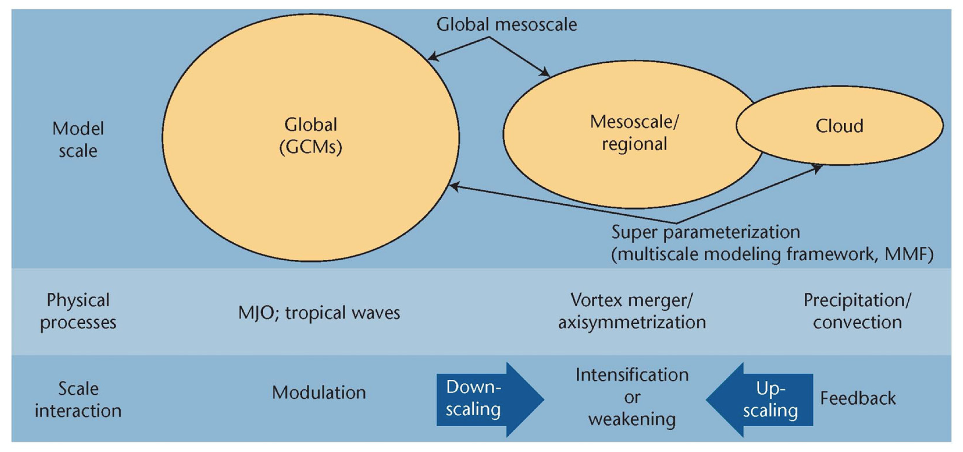
Downscaling itself has practical applications for deriving features at small scales. Recent research in real-world multiscale modeling and analysis (Shen et al., 2013 [75]; Frank and Roundy 2006 [77]) indicates that large-scale processes can modulate small-scale chaos, potentially extending predictability. For example, as shown in Figure 12, findings from our real-world models (Shen et al., 2010) [38], later supported by chaotic modeling, indicate that accurate representations of both downscaling and upscaling processes could enhance weather and climate predictability. Specifically, the advantage of a global model, as compared to a regional model, lies in its larger scale that can accurately provide downscaling processes. Such an advantage is analogous to the long-range dependencies enabled by the attention mechanism of the transformer technology. Thus, increasing the complexities of scale interactions in weather models is analogous to enhancing long-range dependencies for context predictions using transformer technology in large language models, as suggested by scaling laws (Kaplan et al., 2020 [78]; Llama Team 2024 [79]).
Although this study focuses on the application of the proposed method for weather and climate predictions, I would like to draw readers’ attention to the following potential contribution to understanding the transformer’s strength and weakness. Lorenz’s butterfly effect and chaos theory demonstrate the amplification of errors through iterative processes. The butterfly effect mirrors accumulated error that causes AI model collapse when generated data are used to train new AI models. Consequently, the transformer-based core system could be applied to meticulously examine the onset of the butterfly effect, defined by sensitive dependence on initial conditions (SDIC). This capability is intended to detect the appearance of errors or hallucinations within ML-based models.
While the nonlinear butterfly effect has been applied to “infer” a negative contribution by increasing nonlinearity or model complexities (e.g., parameterizations) to predictability, the scaling law (e.g., Kaplan et al., 2020 [78]; Llama team 2024 [79]) suggests a positive contribution due to increasing data volumes and weight (both of which augment model complexity) enabled by advanced computing power. Although the ML-based core system might be separately trained to analyze downscaling (i.e., control by large-scale variables) and upscaling processes (i.e., feedback by small scale variables), ideally, it is crucial to examine multiscale processes concurrently, considering both the scaling law with long-range dependence and chaos theory with the butterfly effect.
Finally, based on my findings and interpretations (or viewed as a hypothesis), my approach can be applied in the following scenario: Since reanalysis data (Hersbach et al., 2018 [80]) can be considered as observations, weather systems at various scales in the reanalysis data are interconnected. This implies that a system at a specific scale retains memory of impacts from other systems at different scales. By applying a scale decomposition method (e.g., fast Fourier transform or parallel empirical mode decomposition, Wu and Shen 2016) to obtain large- and small-scale systems, such as African easterly waves and hurricanes, these weather systems at different scales can be used to train an empirical model as depicted in Figure 2. Given the need for spatial correlation in addition to temporal correlation, vision transformer (ViT) technology (e.g., Dosovitskiy 2020 [66]), a variant of transformer technology, is an ideal approach for this kind of study.
Eventually, I will integrate the core system into one or two state-of-the-art weather foundation models to use large-scale wind fields or eigenmodes associated with Madden–Julian oscillations (Madden and Julian 1971, 1994 [81,82]), as well as other large-scale systems, as predictors, with smaller features such as regional and local precipitation as outputs. Findings from this approach aim to improve prediction accuracy and explore new possibilities for weather and climate forecasting, potentially challenging traditional predictability limits (Charney et al. 1966 [83]; GARP 1969 [84]; Lorenz 1969a, b, c, 1993 [20,85,86,87]; Reeves 2014 [88]; Shen et al., 2024 [89]).

5. Conclusions

The downscaling technique has been employed to derive detailed features from coarse information. In this study, I illustrate the concept of downscaling using the generalized Lorenz model (GLM) combined with machine learning (ML)-based empirical models. My research spans multiple disciplines, including atmospheric sciences, nonlinear dynamics, and ML methodologies. The newly developed GLM was utilized to generate irregular chaotic data at two or three spatial scales for training and validation. Primary and secondary scale variables, representing larger and smaller scale data, respectively, were used as inputs and outputs. Three major types of ML-based models were developed: a linear regression model, a feedforward neural network (FFNN) model, and a transformer-based model. All three models demonstrated strong performance, with correlation coefficients between the predicted and true (i.e., GLM-simulated) small-scale variables exceeding 0.9. The transformer-based model, which produced better results than the other two models, showed good performance in both control and parallel runs where sensitive dependence on initial conditions (SDIC, also known as the butterfly effect) was evident during the validation period. While Lorenz’s groundbreaking study “Deterministic Nonperiodic Flow” suggests finite predictability, my finding that irregular, non-periodic small-scale variables can be reliably estimated using multiple non-periodic large-scale variables indicates the feasibility of downscaling within chaotic Lorenz systems.
My earlier study (Shen 2016) demonstrated hierarchical scale dependence by examining the time-averaged correlation of “true” (simulated) variables at different scales. In this study, ML-based models were developed to “predict” time series of small-scale variables and illustrate their connection to the true small-scale variables. Specifically, the temporal variations of two variables and their correlation coefficients during the training or validation period were discussed. Consequently, this study, along with my previous research, collectively provides a theoretical foundation for downscaling within chaotic Lorenz models. However, as discussed in Section 4, these findings must be interpreted with caution. Future work, which is also presented in Section 4, includes the extension of the current core system to reveal upscaling processes within the generalized model and integration of the core system into existing AI weather foundation models to explore new predictability horizons in weather and climate.

Funding

This research received no external funding.

Data Availability Statement

Python code for the GLM and empirical models available upon request.

Acknowledgments

We thank the three anonymous reviewers, academic editors, and editors for valuable comments and discussions.

Conflicts of Interest

The author declares no conflicts of interest.

References

  1. Wilby, R.L.; Wigley, T.M.L. Downscaling general circulation model output: A review of methods and limitations. Prog. Phys. Geogr. 1997, 21, 530–548. [Google Scholar] [CrossRef]
  2. Castro, C.L.; Pielke, R.A., Sr.; Leoncini, G. Dynamical downscaling: Assessment of value retained and added using the Regional Atmospheric Modeling System (RAMS). J. Geophys. Res.—Atmos. 2005, 110, D05108. [Google Scholar] [CrossRef]
  3. Maraun, D.; Wetterhall, F.; Ireson, A.M.; Chandler, R.E.; Kendon, E.J.; Widmann, M.; Brienen, S.; Rust, H.W.; Sauter, T.; Themessl, M.; et al. Precipitation Downscaling under climate change. Recent developments to bridge the gap between dynamical models and the end user. Rev. Geophys. 2010, 48, RG3003. [Google Scholar] [CrossRef]
  4. Pielke, R.A., Sr.; Wilby, R.L. Regional climate downscaling—What’s the point? Eos Forum 2012, 93, 52–53. [Google Scholar] [CrossRef]
  5. Juang, H.-M.H.; Kanamitsu, M. The NMC Regional Spectral Model. Mon. Weather Rev. 1994, 122, 3–26. [Google Scholar] [CrossRef]
  6. Von Storch, H.; Langenberg, H.; Feser, F. A spectral nudging technique for dynamical downscaling purposes. Mon. Weather Rev. 2000, 128, 3664–3673. [Google Scholar] [CrossRef]
  7. Pathak, J.; Subramanian, S.; Harrington, P.; Raja, S.; Chattopadhyay, A.; Mardani, M.; Kurth, T.; Hall, D.; Li, Z.; Azizzadenesheli, K.; et al. Fourcastnet: A Global Data-Driven High-Resolution Weather Model Using Adaptive Fourier Neural Operators. arXiv 2022, arXiv:2202.11214. [Google Scholar]
  8. Bi, K.; Xie, L.; Zhang, H.; Chen, X.; Gu, X.; Tian, Q. Accurate medium-range global weather forecasting with 3D neural networks. Nature 2023, 619, 533–538. [Google Scholar] [CrossRef]
  9. Bonev, B.; Kurth, T.; Hundt, C.; Pathak, J.; Baust, M.; Kashinath, K.; Anandkumar, A. Spherical Fourier Neural Operators: Learning Stable Dynamics on the Sphere. arXiv 2023, arXiv:2306.03838. [Google Scholar] [CrossRef]
  10. Chen, K.; Han, T.; Gong, J.; Bai, L.; Ling, F.; Luo, J.-J.; Chen, X.; Ma, L.; Zhang, T.; Su, R.; et al. FengWu: Pushing the Skillful Global Medium-range Weather Forecast beyond 10 Days Lead. arXiv 2023, arXiv:2304.02948. [Google Scholar]
  11. Chen, L.; Zhong, X.; Zhang, F.; Cheng, Y.; Xu, Y.; Qi, Y.; Li, H. FuXi: A cascade machine learning forecasting system for 15-day global weather forecast. NPJ Clim. Atmos. Sci. 2023, 6, 190. [Google Scholar] [CrossRef]
  12. Nguyen, T.; Brandstetter, J.; Kapoor, A.; Gupta, J.K.; Grover, A. Climax: A Foundation Model for Weather and Climate. In Proceedings of the Workshop “Tackling Climate Change with Machine Learning, ICLR 2023, Virtual, 9 December 2022. [Google Scholar]
  13. Selz, T.; Craig, G.C. Can artificial intelligence-based weather prediction models simulate the butterfly effect? Geophys. Res. Lett. 2023, 50, e2023GL105747. [Google Scholar] [CrossRef]
  14. Watt-Meyer, O.; Dresdner, G.; McGibbon, J.; Clark, S.K.; Henn, B.; Duncan, J.; Brenowitz, N.D.; Kashinath, K.; Pritchard, M.S.; Bonev, B.; et al. ACE: A fast, skillful learned global atmospheric model for climate prediction. arXiv 2023, arXiv:2310.02074v1. [Google Scholar] [CrossRef]
  15. Bouallègue, Z.B.; Clare, M.C.A.; Magnusson, L.; Gascon, E.; Maier-Gerber, M.; Janousek, M.; Rodwell, M.; Pinault, F.; Dramsch, J.S.; Lang, S.T.K.; et al. The rise of data-driven weather forecasting: A first statistical assessment of machine learning-based weather forecasts in an operational-like context. Bull. Am. Meteorol. Soc. 2024, 105, E864–E883. [Google Scholar] [CrossRef]
  16. Li, H.; Chen, L.; Zhong, X.; Wu, J.; Chen, D.; Xie, S.-P.; Chao, Q.; Lin, C.; Hu, Z.; Lu, B.; et al. A machine learning model that outperforms conventional global subseasonal forecast models. Nat. Portf. 2024. [Google Scholar] [CrossRef]
  17. Wiener, N. Nonlinear prediction and dynamics. In Proceeding of the Third Berkeley Symposium on Mathematics, Statistics, and Probability, Statistical Laboratory of the University of California, Berkeley, CA, USA, 26–31 December 1954; University of California Press: Berkeley, CA, USA, 1956; Volume III, pp. 247–252. [Google Scholar]
  18. Charney, J.; Fjørtoft, R.; von Neumann, J. Numerical Integration of the Barotropic Vorticity Equation. Tellus 1950, 2, 237. [Google Scholar] [CrossRef]
  19. Lorenz, E.N. The statistical prediction of solutions of dynamic equations. In Proceedings of the International Symposium on Numerical Weather Prediction, Tokyo, Japan, 7–13 November 1962; pp. 629–635. [Google Scholar]
  20. Lorenz, E.N. The Essence of Chaos; University of Washington Press: Seattle, WA, USA, 1993; 227p. [Google Scholar]
  21. Shen, B.-W.; Pielke, R.A., Sr.; Zeng, X. 50th Anniversary of the Metaphorical Butterfly Effect since Lorenz (1972): Special Issue on Multistability, Multiscale Predictability, and Sensitivity in Numerical Models. Atmosphere 2023, 14, 1279. [Google Scholar] [CrossRef]
  22. Saltzman, B. Finite Amplitude Free Convection as an Initial Value Problem-I. J. Atmos. Sci. 1962, 19, 329–341. [Google Scholar] [CrossRef]
  23. Lorenz, E.N. Deterministic nonperiodic flow. J. Atmos. Sci. 1963, 20, 130–141. [Google Scholar] [CrossRef]
  24. Lakshmivarahan, S.; Lewis, J.M.; Hu, J. Saltzman’s Model: Complete Characterization of Solution Properties. J. Atmos. Sci. 2019, 76, 1587–1608. [Google Scholar] [CrossRef]
  25. Lewis, J.M.; Sivaramakrishnan, L. Role of the Observability Gramian in Parameter Estimation: Application to Nonchaotic and Chaotic Systems via the Forward Sensitivity Method. Atmosphere 2022, 13, 1647. [Google Scholar] [CrossRef]
  26. Gleick, J. Chaos: Making a New Science; Penguin: New York, NY, USA, 1987; 360p. [Google Scholar]
  27. Li, T.-Y.; Yorke, J.A. Period Three Implies Chaos. Am. Math. Mon. 1975, 82, 985–992. [Google Scholar] [CrossRef]
  28. Curry, J.H. Generalized Lorenz systems. Commun. Math. Phys. 1978, 60, 193–204. [Google Scholar] [CrossRef]
  29. Curry, J.H.; Herring, J.R.; Loncaric, J.; Orszag, S.A. Order and disorder in two- and three-dimensional Benard convection. J. Fluid Mech. 1984, 147, 1–38. [Google Scholar] [CrossRef]
  30. Howard, L.N.; Krishnamurti, R.K. Large-scale flow in turbulent convection: A mathematical model. J. Fluid Mech. 1986, 170, 385–410. [Google Scholar] [CrossRef]
  31. Hermiz, K.B.; Guzdar, P.N.; Finn, J.M. Improved low-order model for shear flow driven by Rayleigh–Benard convection. Phys. Rev. E 1995, 51, 325–331. [Google Scholar] [CrossRef]
  32. Thiffeault, J.-L.; Horton, W. Energy-conserving truncations for convection with shear flow. Phys. Fluids 1996, 8, 1715–1719. [Google Scholar] [CrossRef]
  33. Musielak, Z.E.; Musielak, D.E.; Kennamer, K.S. The onset of chaos in nonlinear dynamical systems determined with a new fractal technique. Fractals 2005, 13, 19–31. [Google Scholar] [CrossRef]
  34. Roy, D.; Musielak, Z.E. Generalized Lorenz models and their routes to chaos. I. Energy-conserving vertical mode truncations. Chaos Solit. Fract. 2007, 32, 1038–1052. [Google Scholar] [CrossRef]
  35. Roy, D.; Musielak, Z.E. Generalized Lorenz models and their routes to chaos. II. Energyconserving horizontal mode truncations. Chaos Solit. Fract. 2007, 31, 747–756. [Google Scholar] [CrossRef]
  36. Roy, D.; Musielak, Z.E. Generalized Lorenz models and their routes to chaos. III. Energyconserving horizontal and vertical mode truncations. Chaos Solit. Fract. 2007, 33, 1064–1070. [Google Scholar] [CrossRef]
  37. Moon, S.; Han, B.-S.; Park, J.; Seo, J.M.; Baik, J.-J. Periodicity and chaos of high-order Lorenz systems. Int. J. Bifurc. Chaos 2017, 27, 1750176. [Google Scholar] [CrossRef]
  38. Shen, B.-W.; Tao, W.-K.; Wu, M.-L. African Easterly Waves in 30-day High-resolution Global Simulations: A Case Study during the 2006 NAMMA Period. Geophys. Res. Lett. 2010, 37, L18803. [Google Scholar] [CrossRef]
  39. Shen, B.-W.; Tao, W.-K.; Green, B. Coupling Advanced Modeling and Visualization to Improve High-Impact Tropical Weather Prediction (CAMVis). IEEE Comput. Sci. Eng. (CiSE) 2011, 13, 56–67. [Google Scholar] [CrossRef]
  40. Shen, B.-W. Nonlinear Feedback in a Five-dimensional Lorenz Model. J. Atmos. Sci. 2014, 71, 1701–1723. [Google Scholar] [CrossRef]
  41. Shen, B.-W. Hierarchical scale dependence associated with the extension of the nonlinear feedback loop in a seven-dimensional Lorenz model. Nonlin. Processes Geophys. 2016, 23, 189–203. [Google Scholar] [CrossRef]
  42. Shen, B.-W. Aggregated Negative Feedback in a Generalized Lorenz Model. Int. J. Bifurc. Chaos 2019, 29, 1950037. [Google Scholar] [CrossRef]
  43. Shen, B.-W. On the Predictability of 30-day Global Mesoscale Simulations of Multiple African Easterly Waves during Summer 2006: A View with a Generalized Lorenz Model. Geosciences 2019, 9, 281. [Google Scholar] [CrossRef]
  44. Felicio, C.C.; Rech, P.C. On the dynamics of five- and six-dimensional Lorenz models. J. Phys. Commun. 2018, 2, 025028. [Google Scholar] [CrossRef]
  45. Faghih-Naini, S.; Shen, B.-W. Quasi-periodic in the five-dimensional non-dissipative Lorenz model: The role of the extended nonlinear feedback loop. Int. J. Bifurc. Chaos 2018, 28, 1850072. [Google Scholar] [CrossRef]
  46. Reyes, T.; Shen, B.-W. A Recurrence Analysis of Chaotic and Non-Chaotic Solutions within a Generalized Nine-Dimensional Lorenz Model. Chaos Solitons Fractals 2019, 125, 1–12. [Google Scholar] [CrossRef]
  47. Cui, J.; Shen, B.-W. A Kernel Principal Component Analysis of Coexisting Attractors within a Generalized Lorenz Model. Chaos Solitons Fractals 2021, 146, 110865. [Google Scholar] [CrossRef]
  48. Rosenblatt, F. The perceptron: A probabilistic model for information storage and organization in the brain. Psychol. Rev. 1958, 65, 386–408. [Google Scholar] [CrossRef] [PubMed]
  49. Rumelhart, D.E.; Hinton, G.E.; Williams, R.J. Learning representations by back propagating errors. Nature 1986, 323, 533–536. [Google Scholar] [CrossRef]
  50. LeCun, Y.; Bottou, L.; Bengio, Y.; Haffner, P. Gradient-based learning applied to document recognition. Proc. IEEE 1998, 86, 2278–2324. [Google Scholar] [CrossRef]
  51. Krizhevsky, A.; Sutskever, I.; Hinton, G.E. ImageNet classification with deep convolutional neural networks. In Advances in Neural Information Processing Systems; MIT Press: Cambridge, MA, USA, 2012; pp. 1097–1105. Available online: https://papers.nips.cc/paper/2012/hash/c399862d3b9d6b76c8436e924a68c45b-Abstract.html (accessed on 4 July 2024).
  52. Elman, J.L. Finding structure in time. Cogn. Sci. 1990, 14, 179–211. [Google Scholar] [CrossRef]
  53. Hochreiter, S.; Schmidhuber, J. Long short-term memory. Neural Comput. 1997, 9, 1735–1780. [Google Scholar] [CrossRef]
  54. Atienza, R. Advanced Deep Learning with Tensorflow 2 and Keras, 2nd ed.; Packt Publishing Ltd.: Brimingham, UK, 2020; 491p. [Google Scholar]
  55. Theodoridis, S. Machine Learning: A Bayesian and Optimization Perspective, 2nd ed.; Ellsevier Ltd.: London, UK, 2020; 1131p. [Google Scholar]
  56. Vaswani, A.; Shazeer, N.; Parmar, N.; Uszkoreit, J.; Jones, L.; Gomez, A.N.; Kaiser, Ł.; Polosukhin, I. Attention is All You Need; Advances in Neural Information Processing Systems. 30; Curran Associates, Inc.: Red Hook, NY, USA, 2017; Available online: https://proceedings.neurips.cc/paper/2017/file/3f5ee243547dee91fbd053c1c4a845aa-Paper.pdf (accessed on 4 July 2024).
  57. Raschka, S.; Liu, Y.H.; Mirjalili, V. Machine Learning with Pytorch and Scikit-Learn; Packt Publishing Ltd.: Brimingham, UK, 2022; 741p. [Google Scholar]
  58. Bommasani, R.; Hudson, D.A.; Adeli, E.; Altman, R.; Arora, S.; von Arx, S.; Bernstein, M.S.; Bohg, J.; Bosselut, A.; Brunskill, E.; et al. On the Opportunities and Risks of Foundation Models. arXiv 2022, arXiv:2108.07258. [Google Scholar] [CrossRef]
  59. OpenAI. ChatGPT 3.5: Language Model [Computer Software]. OpenAI. 2023. Available online: https://chat.openai.com/ (accessed on 4 July 2024).
  60. Devlin, J.; Chang, M.-W.; Lee, K.; Toutanova, K. BERT: Pre-Training of Deep Bidirectional Transformers for Language Understanding; Association for Computational Linguistics (ACL): Kerrville, TX, USA, 2019; pp. 4171–4186. [Google Scholar]
  61. Raffel, C.; Shazeer, N.; Roberts, A.; Lee, K.; Narang, S.; Matena, M.; Zhou, Y.; Li, W.; Liu, P.J. Exploring the limits of transfer learning with a unified text-to-text transformer. arXiv 2019, arXiv:1910.10683. [Google Scholar]
  62. Radford, A.; Wu, J.; Child, R.; Luan, D.; Amodei, D.; Sutskever, I. Language models are unsupervised multitask learners. OpenAI Blog 2019, 1, 8. [Google Scholar]
  63. Yin, P.; Neubig, G.; Yih, W.-t.; Riedel, S. TaBERT: Pretraining for Joint Understanding of Textual and Tabular Data. In Proceedings of the 58th Annual Meeting of the Association for Computational Linguistics, Online, 5–10 July 2020; pp. 8413–8426. [Google Scholar]
  64. Chen, M.; Radford, A.; Child, R.; Wu, J.; Jun, H.; Luan, D.; Sutskever, I. Generative Pretraining from Pixels. In Proceedings of the 37th International Conference on Machine Learning (Proceedings of Machine Learning Research, Vol. 119), Online, 12–18 July 2020; Daumé, H., III, Singh, A., Eds.; PMLR: Boston, MA, USA, 2020; pp. 1691–1703. Available online: http://proceedings.mlr.press/v119/chen20s.html (accessed on 4 July 2024).
  65. Rives, A.; Meier, J.; Sercu, T.; Goyal, S.; Lin, Z.; Liu, J.; Guo, D.; Myle Ott, C.; Zitnick, L.; Ma, J.; et al. Biological structure and function emerge from scaling unsupervised learning to 250 million protein sequences. Proc. Natl. Acad. Sci. USA 2021, 118, 15. [Google Scholar] [CrossRef] [PubMed]
  66. Dosovitskiy, A.; Beyer, L.; Kolesnikov, A.; Weissenborn, D.; Zhai, X.; Unterthiner, T.; Dehghani, M.; Minderer, M.; Heigold, G.; Gelly, S.; et al. An Image is Worth 16x16 Words: Transformers for Image Recognition at Scale. arXiv 2020, arXiv:2010.11929. [Google Scholar] [CrossRef]
  67. Shen, B.-W.; Pielke, R.A., Sr.; Zeng, X.; Baik, J.-J.; Faghih-Naini, S.; Cui, J.; Atlas, R. Is weather chaotic? Coexistence of chaos and order within a generalized Lorenz model. Bull. Am. Meteorol. Soc. 2021, 2, E148–E158. [Google Scholar] [CrossRef]
  68. Pedlosky, J. Finite-amplitude baroclinic waves with small dissipation. J. Atmos. Sci. 1971, 28, 587597. [Google Scholar] [CrossRef]
  69. Pauli, V.; Gommers, R.; Oliphant, T.E.; Haberland, M.; Reddy, T.; Cournapeau, D.; Burovski, E.; Peterson, P.; Weckesser, W.; Bright, J.; et al. SciPy 1.0: Fundamental Algorithms for Scientific Computing in Python. Nat. Methods 2020, 17, 261–272. [Google Scholar]
  70. Shen, B.-W.; Pielke, R.A., Sr.; Zeng, X.; Cui, J.; Faghih-Naini, S.; Paxson, W.; Atlas, R. Three Kinds of Butterfly Effects Within Lorenz Models. Encyclopedia 2022, 2, 1250–1259. [Google Scholar] [CrossRef]
  71. Pielke, R.A.; Shen, B.-W.; Zeng, X. Butterfly Effects. Phys. Today 2024, 77, 10. [Google Scholar] [CrossRef]
  72. Lighthill, J. The recently recognized failure of predictability in Newtonian dynamics. Proc. R. Soc. Lond. A 1986, 407, 35–50. [Google Scholar]
  73. Shen, B.-W. A Review of Lorenz’s Models from 1960 to 2008. Int. J. Bifurc. Chaos 2023, 33, 2330024. [Google Scholar] [CrossRef]
  74. He, K.; Zhang, X.; Ren, S.; Sun, J. Deep Residual Learning for Image Recognition. arXiv 2015, arXiv:1512.03385. [Google Scholar] [CrossRef]
  75. Shen, B.-W.; Nelson, B.; Cheung, S.; Tao, W.-K. Improving the NASA Multiscale Modeling Framework’s Performance for Tropical Cyclone Climate Study. Comput. Sci. Eng. 2013, 5, 56–67. [Google Scholar] [CrossRef]
  76. Wu, Y.-L.; Shen, B.-W. An Evaluation of the Parallel Ensemble Empirical Mode Decomposition Method in Revealing the Role of Downscaling Processes Associated with African Easterly Waves in Tropical Cyclone Genesis. J. Atmos. Oceanic Technol. 2016, 33, 1611–1628. [Google Scholar] [CrossRef]
  77. Frank, W.M.; Roundy, P.E. The role of tropical waves in tropical cyclogenesis. Mon. Weather Rev. 2006, 134, 2397–2417. [Google Scholar] [CrossRef]
  78. Kaplan, J.; McCandlish, S.; Henighan, T.; Brown, T.B.; Chess, B.; Child, R.; Gray, S.; Radford, A.; Wu, J.; Amodei, D. Scaling Laws for Neural Languages Models. arXiv 2020, arXiv:2001.08361. [Google Scholar] [CrossRef]
  79. Llama Team. The Llama 3 Herd of Models. 2024. Available online: https://llama.meta.com/ (accessed on 4 July 2024).
  80. Hersbach, H.; Bell, B.; Berrisford, P.; Biavati, G.; Horányi, A.; Sabater, J.M.; Nicolas, J.; Peubey, C.; Radu, R.; Rozum, I.; et al. ERA5 Hourly Data on Single Levels from 1979 to Present; Copernicus Climate Change Service (C3S), Climate Data Store (CDS): Reading, UK, 2018; p. 10. [Google Scholar]
  81. Madden, R.A.; Julian, P.R. Detection of a 40–50 day oscillation in the zonal wind in the tropical Pacific. J. Atmos. Sci. 1971, 28, 702–708. [Google Scholar] [CrossRef]
  82. Madden, R.A.; Julian, P.R. Observations of the 40–50-Day Tropical Oscillation—A Review. Mon. Weather Rev. 1994, 122, 814–837. [Google Scholar] [CrossRef]
  83. Charney, J.G.; Fleagle, R.G.; Lally, V.E.; Riehl, H.; Wark, D.Q. The feasibility of a global observation and analysis experiment. Bull. Am. Meteorol. Soc. 1966, 47, 200–220. [Google Scholar]
  84. GARP. GARP topics. Bull. Am. Meteorol. Soc. 1969, 50, 136–141. [Google Scholar]
  85. Lorenz, E.N. Three approaches to atmospheric predictability. Bull. Am. Meteorol. Soc. 1969, 50, 345–351. [Google Scholar]
  86. Lorenz, E.N. Atmospheric predictability as revealed by naturally occurring analogues. J. Atmos. Sci. 1969, 26, 636–646. [Google Scholar] [CrossRef]
  87. Lorenz, E.N. The predictability of a flow which possesses many scales of motion. Tellus 1969, 21, 19. [Google Scholar]
  88. Reeves, R.W. Edward Lorenz Revisiting the Limits of Predictability and Their Implications: An Interview from 2007. Bull. Am. Meteorol. Soc. 2014, 95, 681–687. [Google Scholar] [CrossRef]
  89. Shen, B.-W.; Pielke, R.A., Sr.; Zeng, X.; Zeng, X. Exploring the Origin of the Two-Week Predictability Limit: A Revisit of Lorenz’s Predictability Studies in the 1960s. Atmosphere 2024, 15, 837. [Google Scholar] [CrossRef]
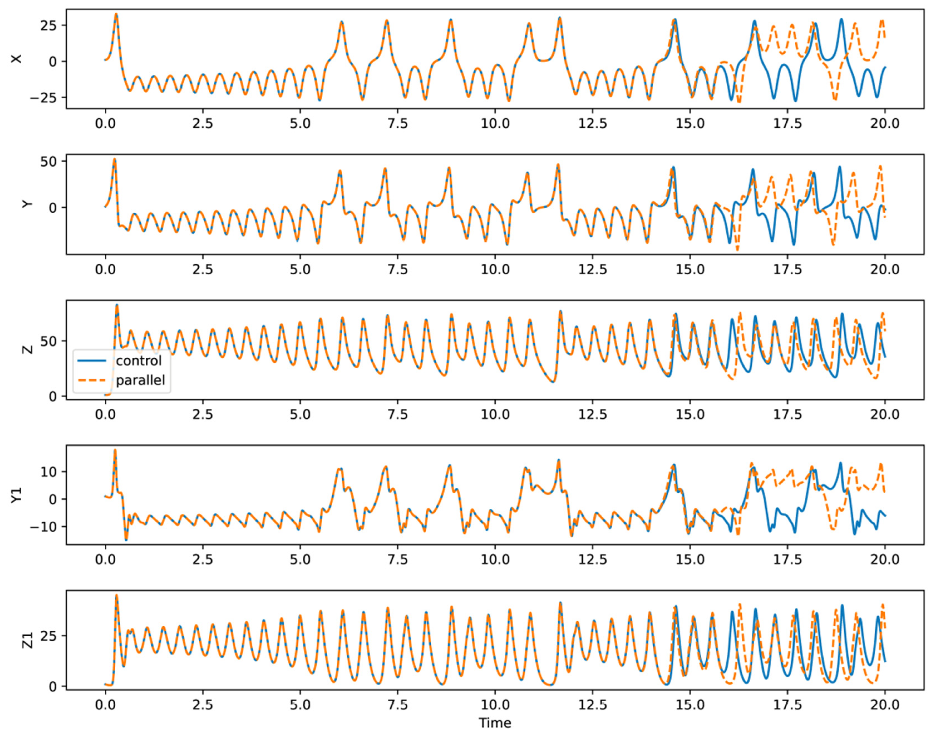
Figure 1. Solutions of the control and parallel runs using the five-dimensional generalized Lorenz model (5DLM), demonstrating sensitive dependence on initial conditions. The two runs differ by a minute initial value of Y, with a difference of 10−5. From top to bottom, the panels show the variables (X, Y, Z) at the primary scale and (Y1, Z1) at the secondary scale.
Make 06 00107 g001
Figure 2. The flowchart illustrates a process where the input variables X, Y, Z, from the generalized Lorenz model (GLM) are fed into a machine learning (ML-based) model. This model can be a linear regression (LinReg), a feedforward neural network (FFNN), or a transformer model. The output variables Y1, Z1 from the GLM, used for training, are then produced by the ML-based model.
Make 06 00107 g002
Figure 3. A diagram with an input layer (X, Y, Z) and an output layer (Y1).
Make 06 00107 g003
Figure 4. Estimates of the secondary scale variable Y1 using the linear regression (LinReg) model (shown in red) and the simple perceptron (SP) model (shown in blue). Both models are based on the architecture shown in Figure 3. The top two panels display results for the training period, while the bottom panels show results for the validation period. The label ’corr’ on the top left of each panel indicates the correlation coefficient between the two variables within the panel.
Make 06 00107 g004
Figure 5. A feedforward neural network (FFNN) with an input layer (X, Y, Z), two hidden layers (each containing 10 units), and an output layer (Y1, Z1).
Make 06 00107 g005
Figure 6. Estimates of the secondary scale variables Y1 and Z1 using the FFNN-based model, constructed based on the architecture shown in Figure 5. Except for the inclusion of the additional variable Z1, the rest is the same as in Figure 4.
Make 06 00107 g006
Figure 7. A transformer-based model illustrating the flow from input variables (X, Y, Z) through an embedding layer (dimension = 64), positional encoding (dimension = 64), three transformer decoder layers (each with dimension = 64), a feedforward network (dimension = 64), and finally to the output variables (Y1, Z1).
Make 06 00107 g007
Figure 8. Similar to Figure 6, but using the transformer-based model instead.
Make 06 00107 g008
Figure 9. Similar to Figure 8, but using the parallel run data instead.
Make 06 00107 g009
Figure 10. Solutions from the seven-dimensional generalized Lorenz model (7DLM). From top to bottom, the panels show the variables (X, Y, Z) at the primary scale, (Y1, Z1) at the secondary scale, and (Y2, Z2) at the tertiary scale.
Make 06 00107 g010
Figure 11. Similar to Figure 8, but using the 7DLM data to train a different transformer-based model.
Make 06 00107 g011
Figure 12. A conceptual model representing interactions across three atmospheric scales. (Top) The three primary categories of Earth’s atmospheric modeling, from left to right: global (large) scale, mesoscale (medium) scale, and cloud (micro) scale. (Middle) The three major weather systems corresponding to each scale. (Bottom) Interactions among the three scales, including downscaling from large-scale systems and upscaling from microscale systems. Strategically, zoomed-out and zoomed-in approaches can effectively capture downscaling and upscaling processes. These approaches align with the principles of scaling law and chaos theory. (Adapted from Shen et al., 2013 [75]).
Make 06 00107 g012
Table 1. Pearson correlation coefficients between the predicted and actual values of variable Y1 over the training and validation periods, using the linear regression (LinReg) model, the feedforward neural network (FFNN) model, and the transformer model. The first two models are provided to verify the performance of the transformer-based model.
ModelTraining PeriodValidation Period
LinReg0.9200.910
FFNN0.9890.988
Transformer0.9930.991
Table 2. Relative RMSE between the predicted and actual values of variable Y1 over the training, using the linear regression (LinReg) model, the feedforward neural network (FFNN) model, and the transformer model. The first two models are provided to verify the performance of the transformer-based model.
ModelTraining Period
LinReg0.07065
FFNN0.02673
Transformer0.02107
Disclaimer/Publisher’s Note: The statements, opinions and data contained in all publications are solely those of the individual author(s) and contributor(s) and not of MDPI and/or the editor(s). MDPI and/or the editor(s) disclaim responsibility for any injury to people or property resulting from any ideas, methods, instructions or products referred to in the content.