Cross-Validation Visualized: A Narrative Guide to Advanced Methods

Abstract

This study delves into the multifaceted nature of cross-validation (CV) techniques in machine learning model evaluation and selection, underscoring the challenge of choosing the most appropriate method due to the plethora of available variants. It aims to clarify and standardize terminology such as sets, groups, folds, and samples pivotal in the CV domain, and introduces an exhaustive compilation of advanced CV methods like leave-one-out, leave-p-out, Monte Carlo, grouped, stratified, and time-split CV within a hold-out CV framework. Through graphical representations, the paper enhances the comprehension of these methodologies, facilitating more informed decision making for practitioners. It further explores the synergy between different CV strategies and advocates for a unified approach to reporting model performance by consolidating essential metrics. The paper culminates in a comprehensive overview of the CV techniques discussed, illustrated with practical examples, offering valuable insights for both novice and experienced researchers in the field.

1. Introduction

In the ever-evolving field of machine learning (ML), the process of developing, deploying, and monitoring models is complex and multifaceted. A structured approach to navigating this complexity is provided by the Cross-Industry Standard Process for Data Mining (CRISP-DM) [1]. This methodology, developed in the late 1990s, has stood the test of time, offering a robust framework for executing ML projects. It comprises six phases: business understanding, data understanding, data preparation, modeling, evaluation, and deployment. Each phase plays a crucial role in ensuring the successful application of ML techniques to solve real-world problems.

A crucial aspect of the CRISP-DM cycle, particularly in the modeling and evaluation phases, is the practice of cross-validation. Cross-validation (CV) is a technique that helps to estimate the robustness and performance of models [2,3,4]. It is primarily used to predict how a model will perform in a production setting, an essential step given the potential variability of data in real-world scenarios. In CV, the data are divided into partitions, where the model is trained on one partition (we refer to this as $D_{train}$) and its performance is evaluated on a disjoint partition $D_{test}$. In this way, the robustness of the model can be assessed more accurately. This process is repeated multiple times, with different partitions, to reduce variability and ensure a more generalizable model.

In any project that follows the CRISP-DM cycle, there comes a point where an estimation of model performance and robustness is required to decide how to proceed with the project. A model is not robust if it performs poorly on new, unseen data. We refer to this phenomenon as overfitting [5,6]. Overfitted models usually have a low bias, but a high variance and perform poorly when predicting new data. Conversely, it may make sense to use simpler models and accept a higher bias in order to achieve better predictive power. The tradeoff between good performance and low bias is referred to as bias–variance tradeoff [7]. By cross-validating a model, we try to optimize the bias–variance tradeoff. By optimizing, we mean we want to minimize both bias and variance. Usually, if bias is high, variance is low and vice versa.

While examining the literature on machine learning, we observed a significant presence of homonyms and synonyms across the discourse related to cross-validation. To address this issue, this paper compiles a list of terms that are frequently used in connection with cross-validation. This glossary serves to increase clarity in the subsequent section, where we explain different cross-validation techniques and their possible combinations. In addition, we propose a formula that tries to balance the bias–variance tradeoff, addressing a crucial aspect of model evaluation. Further, we summarize all the methods discussed and provide a comprehensive assessment of the advantages and disadvantages of each approach. Finally, we discuss future directions of this research area where we point out that considering performance metrics of subject matter experts is equally important to gain value in ML projects.

Consider a machine learning (ML) or statistics project where your task is to train, evaluate, and deploy a model. Your dataset has groups and samples, and each sample has a timestamp, features, and a target (synonyms: outcome, dependent variable, label). To avoid confusion regarding homo- and synonyms, we provide the following list of definitions:

• Sample s (synonyms: instance, data point): Sample refers to a single unit of observation or record within a dataset.
• Dataset D: The total set of all samples available for training, validating, and testing ML models.
• Set: A batch of samples as a subset of the whole dataset D.
• Fold: A batch of samples as a subset of a Set. The term fold is often used in the context of k-fold CV.
• Group g (synonym: block [8]: A sub-collection of samples that share at least one common characteristic. Within the medical domain, for example, this characteristic could be a treating physician or a certain hospital. If multiple samples from the same patient are given, the patient him- or herself can be considered a group.
• Feature x (synonyms: predictor, input, or explanatory variable): An individual characteristic of the data that are given to the model for predicting the target. We denote the set of all features as X.
• Target y: (synonyms: outcome, dependent variable, or label): Within supervised learning, the property predicted by the model.

For further clarification, we illustrate the presented taxonomy concept on a small dataset in Figure 1.

2. Overview of Cross-Validation Methods

In this section, various methods of CV are explained and visualized in more detail. By hold-out CV, we mean that we first split all available samples into two parts: $D_{train}$ and $D_{test}$. We perform cross-validation within $D_{train}$ and finally test our chosen model in the hold-out $D_{test}$ set. If you also cross-validate the hold-out set, we call this nested CV instead of hold-out CV. We further discuss possible combinations of CV approaches and conclude the section with a simple formula that can be used to target the bias–variance tradeoff and optimize the CV approach through a single number.

2.1. Hold-Out CV Methods

In all different CV approaches, we use a hold-out CV approach, which means we use the train set $D_{train}$ to tune model parameters (this is where the CV actually happens) and the test set $D_{test}$ to finally evaluate a chosen model. This idea goes back to [9]. When splitting the total data into training and test datasets, the size of the test set should be large enough to reflect the true distribution, but small enough to maintain the size of the training set. Common ratios are 80–20 or 70–30 for the split of training and test data. For large datasets, such as 10 million samples, a 99:1 train–test split may suffice, as 10,000 samples could adequately represent the target distribution in the test set. There is no one fits all approach, and the appropriate test size varies with the feature space complexity, use case, and target distribution, necessitating individual evaluation for each scenario.

The allocation of samples into folds and sets can happen at either group or sample level. By sample level, we mean that we do not correct for the distribution of the target (stratification) or assign batches of samples to separate groups during splitting. By group level, we mean that we keep groups separated from each other during validation and testing. To recall, a group is a sub-collection of samples that share a least one common characteristic.

2.1.1. Random Splitting of Samples: K-Fold CV

In previous research [2,4], the “classic” method to gauge model performance involves randomly splitting the dataset into k distinct folds, which is well known as k-fold CV. Here, $k-1$ folds constitute the training folds, while the remaining fold serves as the validation fold. Notably, the idea of randomly splitting samples was first mentioned in 1931 [10].

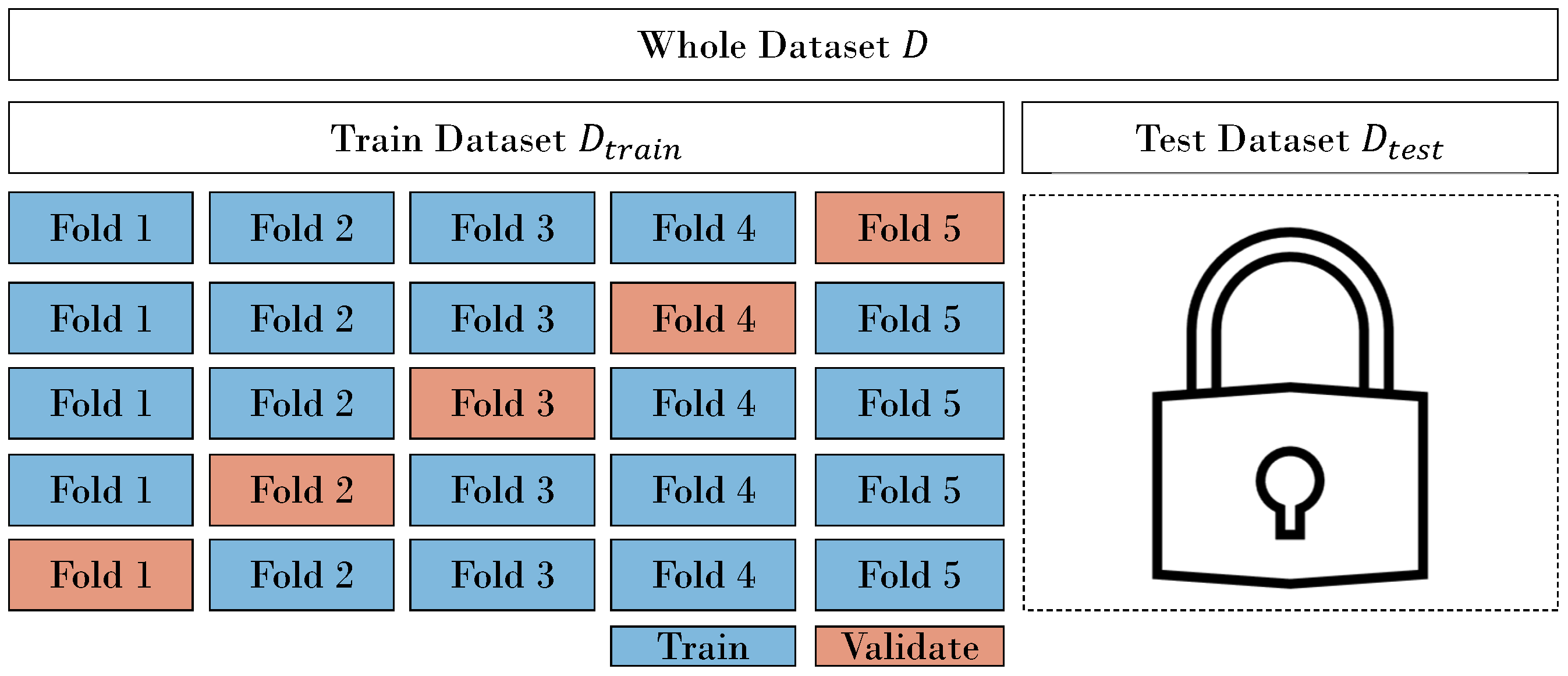
The term validation fold refers to the batch of samples that is used within the train set $D_{train}$ to validate chosen model architectures (see Figure 2). This is not to be confused with a hold-out test set. A test set conclusively evaluates model performance. Depending on the use case you are working on, you might want to reserve a hold-out test set, not utilized for model validation until the end. When we use a validation fold within $D_{train}$ and a hold-out test set $D_{test}$, we call this hold-out CV. Introducing a hold-out test set can help to mitigate overfitting to the dataset D, but it may reduce the available data for model training, potentially affecting the model’s robustness. A hold-out CV approach with random splitting is depicted in Figure 2.

2.1.2. Common Variations of Cross-Validation with Random Splits

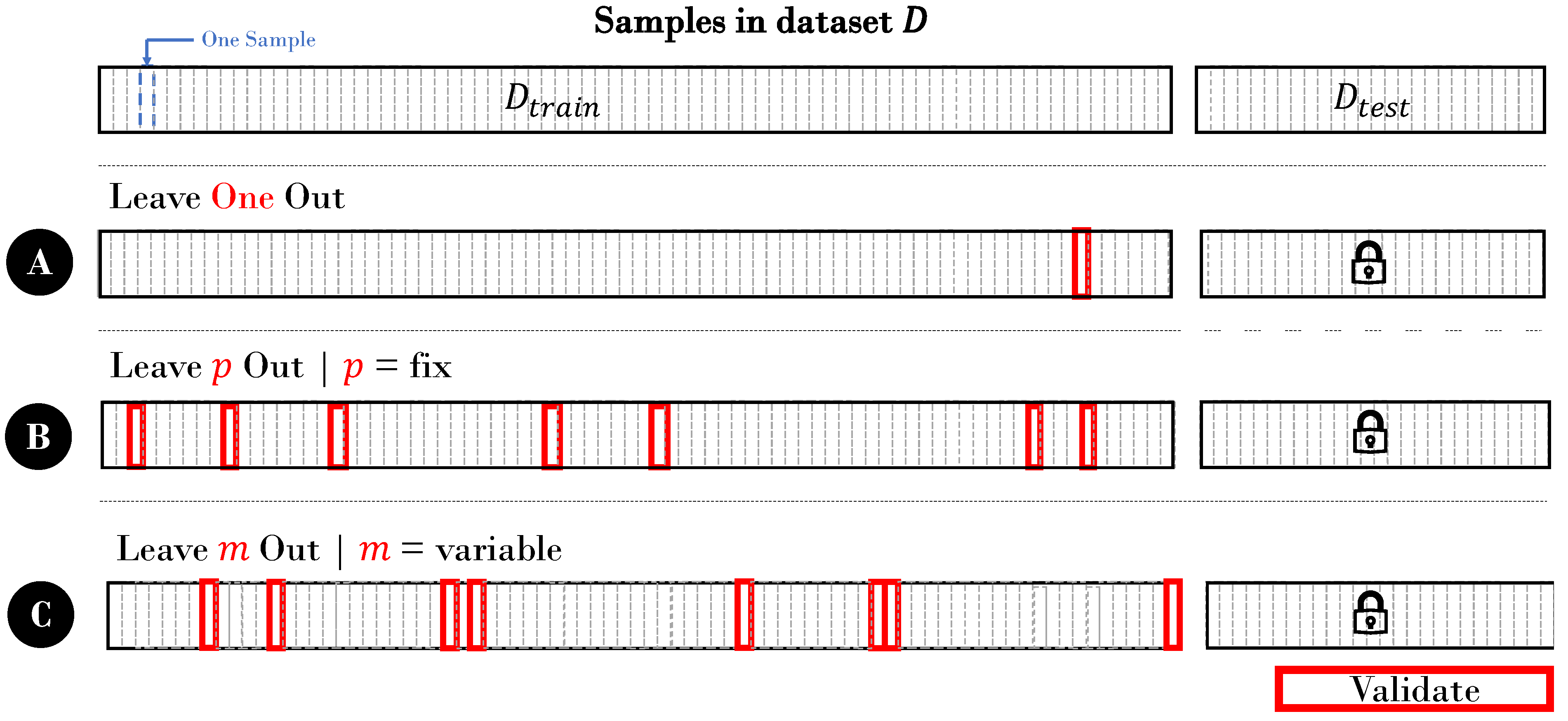
In the previous section, we have seen that we can randomly split the set $D_{train}$ into k folds with each fold equal in size. In this section, we want to summarize three common variations of this approach. In these approaches, the data are not split on a fixed ratio, but on a certain number (1 or p). Note that in classic k-fold CV, each sample is used once. In these variations, however, samples can be used more than once or even not at all. We illustrate these approaches in Figure 3.

Leave-One-Out Cross-Validation

In this approach, all samples except one are used to train the model where the remaining sample is used to validate it. It is useful for smaller datasets where one wants to use as much data as possible to train a more robust model. However, it is also computationally expensive as one has as many validation folds as samples within $D_{train}$. The idea of leaving one sample out for validation of the model was firstly introduced by [9].

Leave-P-Out Cross-Validation

In leave-p-out CV, we leave more than one but less than n samples out to validate our model [11]. n is the number of samples in $D_{train}$. The difference between k-fold CV, leave-one-out CV, and leave-p-out CV lies in the number of samples included in the validation fold: In k-fold CV, each validation fold has $\frac{n}{k}$ samples. In leave-one-out CV, there is only one sample in the validation fold in each iteration, and in leave-p-out CV, you decide the size of the validation fold with p, which can be any value that is not necessarily $\frac{n}{k}$.

The choice of p in leave-p-out CV is a hyperparameter, and selecting an appropriate value for p involves considering the bias–variance tradeoff. Its choice depends on the size of your dataset, the complexity of your model, and the computational resources available. A smaller p leads to lower bias, more computational cost, and high variance. A larger p means lower variance, higher bias, and less data available in the training folds.

Monte Carlo Cross-Validation

The term Monte Carlo is often used in various fields of science and engineering to refer to methods that rely on random sampling. It is inspired by the Monte Carlo Casino in Monaco, known for its games of chance. The Monte Carlo CV (MCCV) approach has one key distinction to the other approaches: Here, the samples in the validation fold are chosen randomly with replacement [12]. That is, samples can overlap between folds. The approach goes back to [13]. Monte Carlo cross-validation (MCCV) is also referred to as Repeated random subsampling validation [14]. We visualize it in Figure 3C. Monte Carlo cross-validation introduces an additional layer of randomness compared to traditional k-fold cross-validation. In classic k-fold CV, the number of samples in each fold remains constant, and the data are randomly split. However, in Monte Carlo CV, not only are the data randomly partitioned, but the number of samples in each fold is also randomly determined. This introduces the possibility of including samples in zero folds or multiple times.

2.1.3. Stratification on the Target

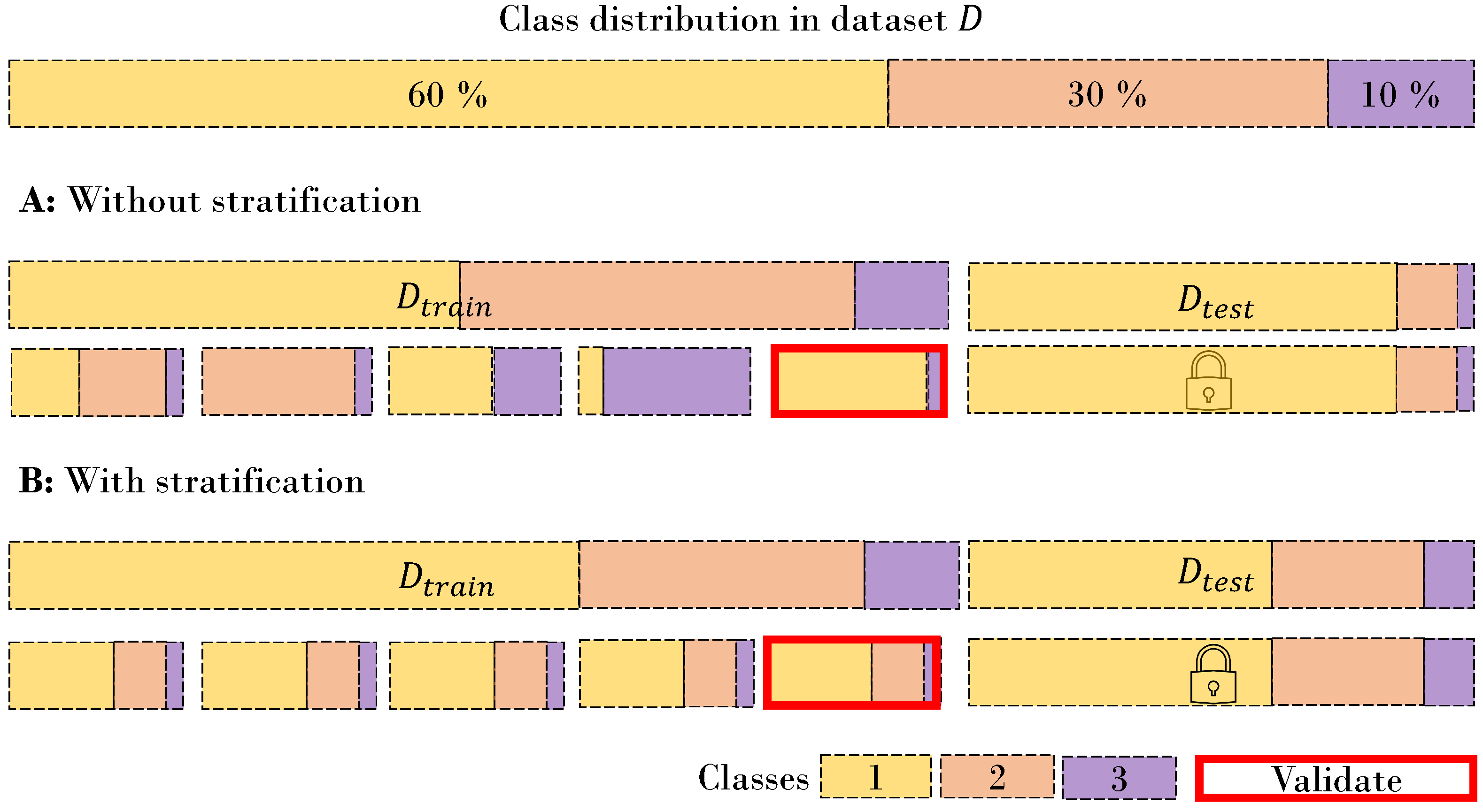
Especially for medical data, it is not uncommon that the target distribution is strongly skewed in one direction, meaning there are many negative cases and only a few positive cases. In medicine, for example, subject matter experts refer to this as prevalence. Prevalence refers to the proportion or percentage of a specific condition or characteristic within a population. In our case, these are samples that refer to a minority class. When performing CV and random splitting, the smaller the batch size of the folds or set, the more likely it is to mitigate a complete class within this set or fold. This is illustrated in Figure 4. When using performance metrics like F1-score, precision, or recall, the observed model performance can significantly fluctuate across folds. This variability is not primarily due to overfitting the data but is rather a result of substantial variations in the target distribution between these folds. You have at least two options to avoid this: Bootstrapping, and using metrics that do not vary due to different class distributions between folds, such as the Area Under The Receiver Operating Characteristic (AUROC). Bootstrap stratification is a resampling technique that retains the original class distribution by generating bootstrap samples. For example, if your original distribution is 10:1 and one of your folds has a distribution of 5:1, you bootstrap the five samples to artificially create that 10:1 ratio.

2.1.4. Grouped Cross-Validation

Grouped or block CV involves aggregating samples into groups. While each group must appear in only one fold, one fold can have several groups. We illustrated this for four groups and one group per fold in Figure 5.

Separating groups helps to prevent overfitting on these groups [8]. One example within the healthcare domain are hospitals: If we group patient data by hospital and ensure that the hospitals are separated during training, the model is more likely to perform well on an unseen hospital after deployment. A broader set of examples may include spatial, hierarchical, and genetic structures [8]. If you have multiple groups that affect model performance, you might want to make this group a feature if that is feasible. For instance, hospital or physician could be a feature. However, if you want to deploy your model in another hospital, hospital cannot be a feature anymore.

2.1.5. Time-Split Cross-Validation

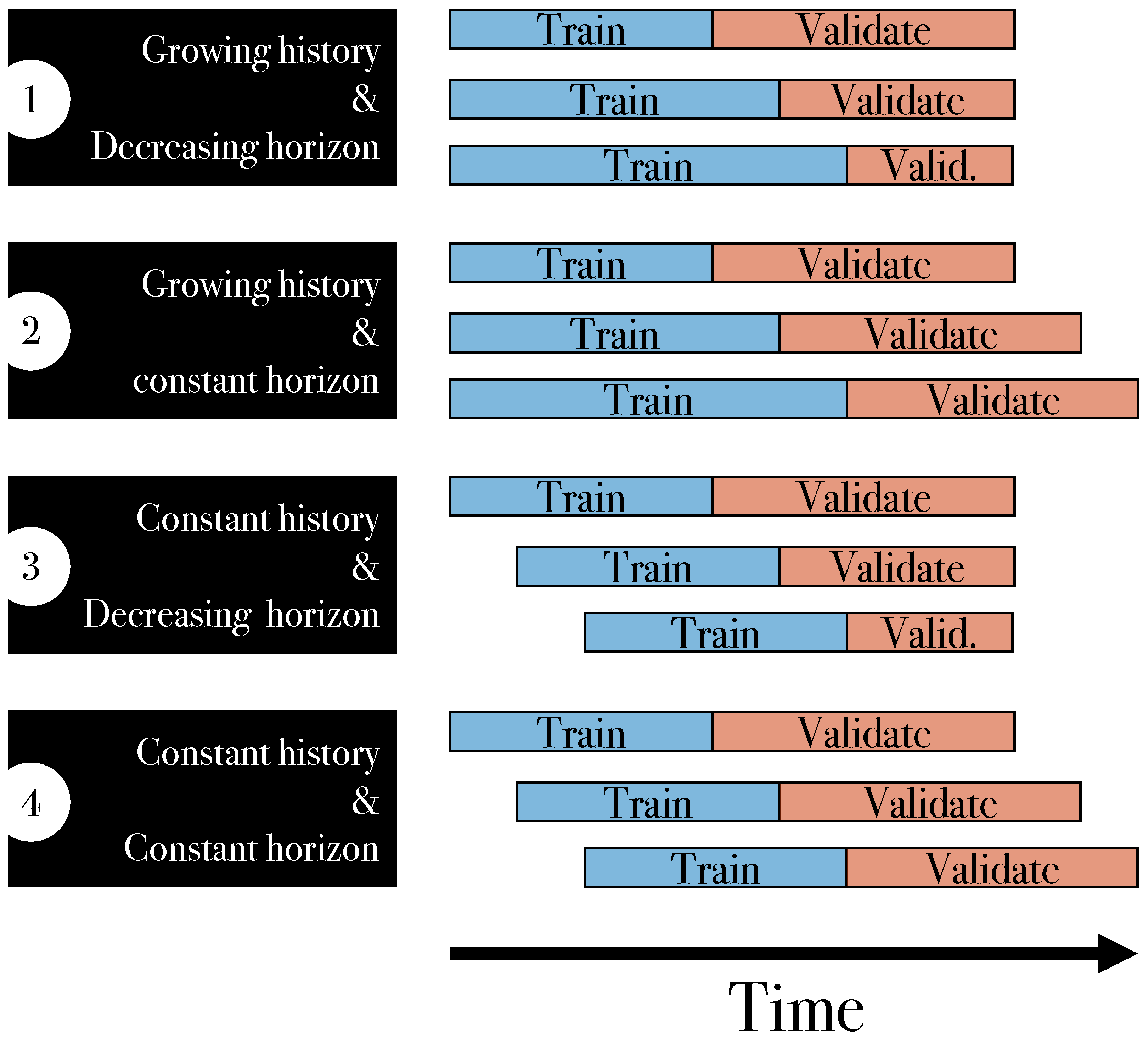
In the introduction, we defined a group as a set of samples that share a common characteristic. If we further know the timestamp of a sample, all samples from the same period of time (a day, a week, a season) can be considered a group [15]. Thus, time-split CV can be considered as a special case of grouped CV. Special for two reasons. First, if you want to train a time-series model, the groups should be ordered by time, and second, groups must not be shuffled during CV. In particular, the validation fold has to contain the “latest” data available at this time. Because we do not shuffle samples or groups, we can also state that this is not cross-validation, but just a train–validate split. However. we can think of four cases in time-split validation, which we drafted in Figure 6.

In scenario 1, the training dataset (=history) expands with each time step, while the validation dataset (=horizon) diminishes. This situation arises when there is a specific future time point of interest. In contrast, in scenario 2, the train data grow, while the size of the validation data remains constant. An example of this is dynamic system handling sensor data in real time with a constant prediction horizon. Scenario 3 mirrors scenario 1, with the exception being that the size of the historical data remains constant instead of growing. Lastly, in scenario 4, both sizes of historical and prospective datasets are fixed. These diverse approaches collectively fall under the umbrella term forward validation [16,17].

Addressing Potential Concept and Data Drift in Time-Split Cross-Validation

Concept drift occurs when the statistical properties of the target variable, which the model is trying to predict, change over time [18]. Data drift, on the other hand, refers to changes in the input data features themselves while keeping the prediction task constant. Especially for longitudinal datasets, the datasets might contain drift. For instance, if the test set contains data that have drifted, given that the folds are stratified and groups are distinct, one can use the time-split approach to check whether the model is robust enough to still perform well in a drifted test set.

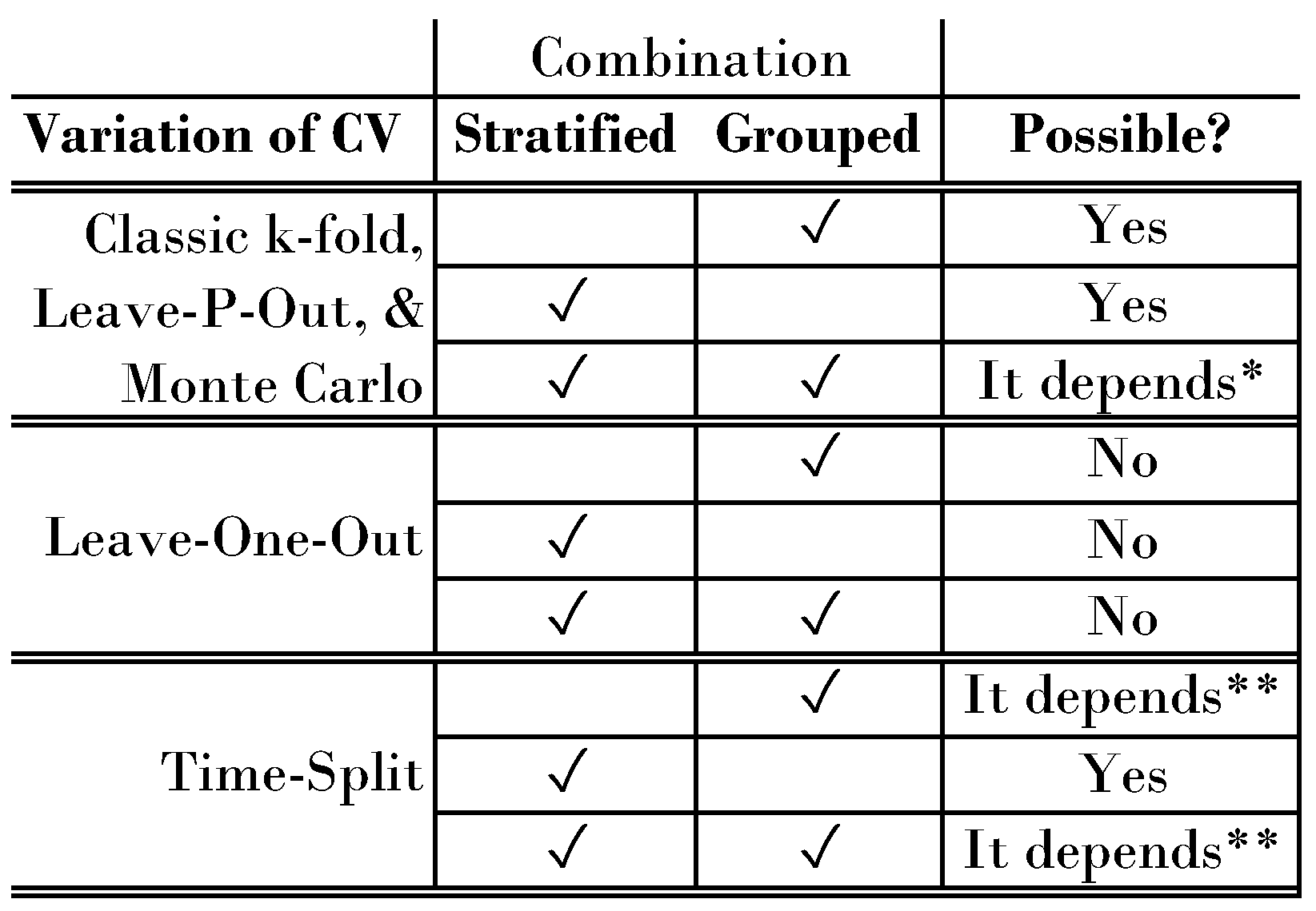
2.2. Limitations on Combining Advanced Methods

In classic k-fold CV, we split samples based on a ratio of $D_{train}$. For instance, a 5-fold CV would assign 20% of the samples to each fold. In contrast, leave-one-out, leave-p-out, and Monte Carlo assign a certain number of samples to the validation fold. When it comes to an extension or combination of the methods, however, we differentiate between the number of samples in the validation fold (1 for leave-one-out, >1 for classic k-fold, leave-p-out, and Monte Carlo). We visualize an overview of possible combinations in Figure 7.

2.3. How to Target the Bias–Variance Trade Off

Up to now, we have mentioned the bias–variance tradeoff several times. In this short section, we offer a formula that might help to handle it. Given k validation folds within $D_{train}$, we can calculate k performance scores $\nu$ and average them. In a validation fold i, we call one performance score ${\nu }_i$.

• ${\overline{\nu }}_{train}=\frac{1}{k}{\sum }_{i=1}^k{\nu }_i$
• To indicate the robustness of the model during training, we can also calculate the standard deviation $\sigma$ as a function of $\nu$:
  $\sigma \left({\nu }_{train}\right)=\sqrt{\frac{1}{k}{\sum }_{i=1}^k{({\nu }_i-{\overline{\nu }}_{train})}^2}$.
• Finally, we can determine the model performance in the test set, ${\nu }_{test}$.

We now have three numbers, the average performance in the training set ${\nu }_{\overline{\mathit{train}}}$, the standard deviation of the model between folds during training, $\sigma \left({\nu }_{train}\right)$, and the test set performance ${\nu }_{test}$. We now can either determine thresholds for two of three numbers and try to optimize the third one, or we combine the numbers to a final score ${\nu }_{final}$ and try to optimize this score. To suggest one combination: ${\nu }_{final}={\nu }_{test}-\sigma \left({\nu }_{train}\right)$. Depending on the use case, one could also add a factor $\alpha$ to the standard deviation score. The more important the model robustness is, the higher $\alpha$ is:

$${\nu }_{final}={\nu }_{test}-\alpha \sigma \left({\nu }_{train}\right)$$

(1)

It is crucial to be mindful of not overfitting our model to the test set $D_{test}$ while fine-tuning for the bias–variance tradeoff. To avoid this, we have two options: limit how often we repeat this step, or introduce a third test set to evaluate the model’s performance after deployment. This ensures the reliability and applicability of our proposed approach.

3. Discussion

In the introduction, we provided a short taxonomy on how to differentiate between datasets, fold, and sets. We differentiated between the sample and group level within CV to obtain more robust models and more accurate estimates of model performance. In the Methods Section, we provided several visualizations for advanced CV methods such as leave-one-out, leave-p-out, and Monte Carlo CV. We showed how stratification and separating groups can help to build more robust models. Next, we considered time-series CV as a special case of grouped CV and showed that here the groups should not be shuffled and the number of training folds increases successively throughout the CV process.

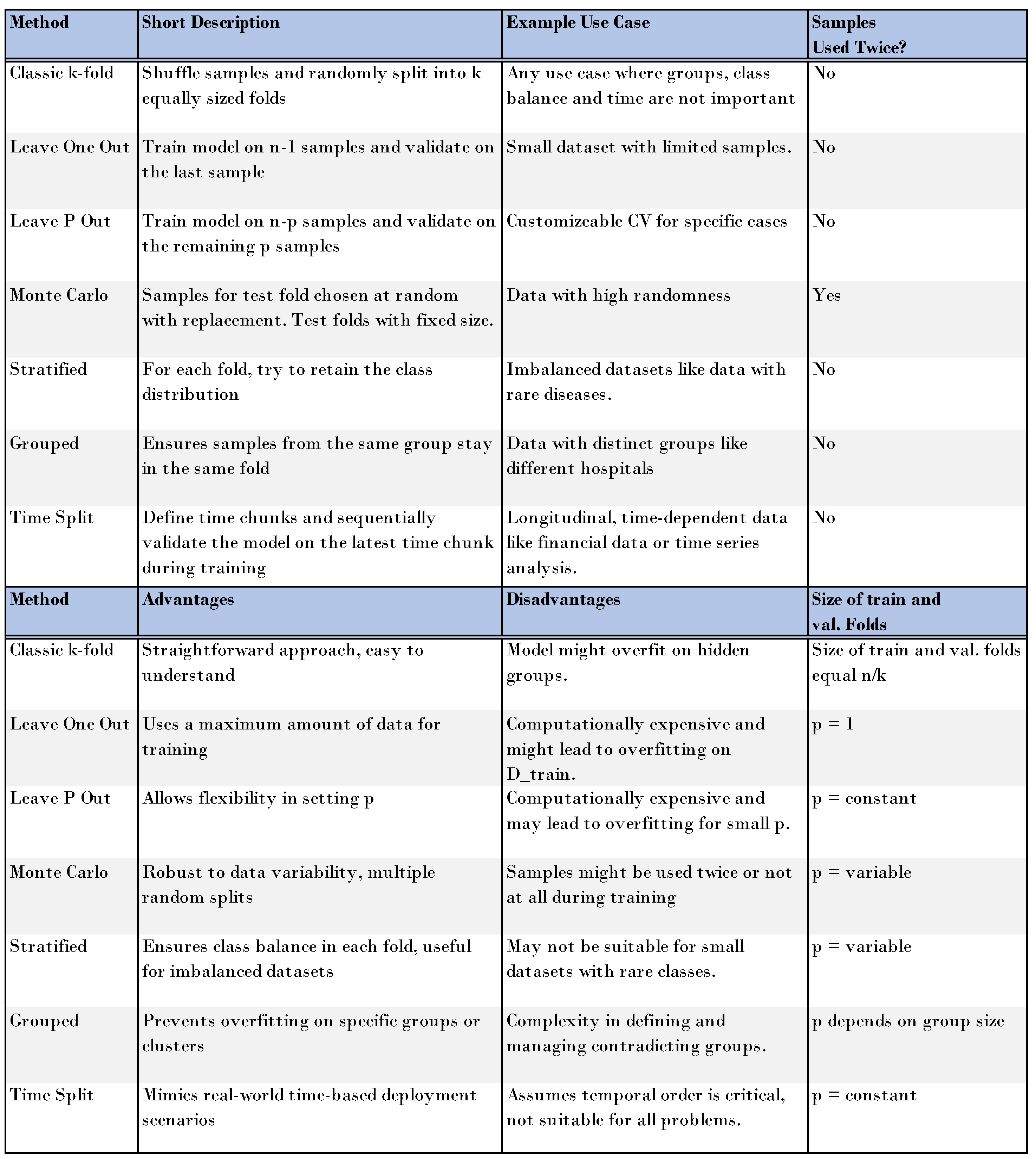
Finally, we provided a template on how to report model performance and explained the options of optimizing either one metric while keeping the others above a threshold, or combining these numbers to a single one while controlling for model robustness via a hyperparameter $\alpha$. We summarize all discussed methods with advantages, disadvantages, and example use cases in Figure 8.

Revisiting the Cross-Industry Standard Process for Data Mining (CRISP-DM) framework outlined in the introduction, it is imperative to acknowledge that selecting an appropriate cross-validation technique or a combination thereof represents merely a fractional component in the overarching schema required for the successful integration of a Machine Learning (ML) model within a production environment. Paramount considerations extend beyond mere methodology to encompass scalability, deployment architecture, and an array of non-technical parameters including legal compliance, transparency, trustworthiness, and the economic ramifications such as return on investment and enhancement of operational workflows, as highlighted by [19]. These dimensions gain clarity and can be more meticulously strategized when underpinned by a precise and reliable estimation of model performance, which is the focal point of this manuscript.

4. Future Directions

Validating machine learning models is essential for assessing their resilience, as highlighted by [19] in their discussion on the challenges of machine learning validation. Our analysis has outlined various validation techniques and their possible integration, underscoring the necessity of evaluating a model’s real-world applicability through its deployment performance. It is critical to acknowledge, as [20] emphasizes, that reliance on simulation-based testing is constrained by the underlying assumptions of the simulations, and thus cannot fully substitute for empirical testing in real-world scenarios. Consequently, we advocate for future studies to investigate the discrepancy between a model’s anticipated performance in testing environments and its actual efficacy in operational contexts. When the objective of a machine learning (ML) project is to enhance value through task automation or workflow simplification, it is crucial to align ML performance metrics with domain-specific relevance. For example, in a healthcare setting where the ML system is tasked with classifying X-ray images, the key question is whether the system effectively identifies straightforward cases, thereby liberating human experts to devote more time to intricate scenarios. Considering this perspective, future research should explore the development of broader connections between domain-specific metrics and ML performance metrics. Specifically, the focus should not solely be on cross-validating through various data splits, but rather on adapting to diverse domain-specific contexts in each of the folds. For instance, treating distinct hospital workflows as unique domain-specific scenarios could be approached through grouped cross-validation. The novelty lies in the approach’s orientation—seeing the ML use case through the subject matter expert’s eyes and translating these needs into different cross-validated sub-use cases.