Quantum-Enhanced Representation Learning: A Quanvolutional Autoencoder Approach against DDoS Threats

Abstract

Motivated by the growing threat of distributed denial-of-service (DDoS) attacks and the emergence of quantum computing, this study introduces a novel “quanvolutional autoencoder” architecture for learning representations. The architecture leverages the computational advantages of quantum mechanics to improve upon traditional machine learning techniques. Specifically, the quanvolutional autoencoder employs randomized quantum circuits to analyze time-series data from DDoS attacks, offering a robust alternative to classical convolutional neural networks. Experimental results suggest that the quanvolutional autoencoder performs similarly to classical models in visualizing and learning from DDoS hive plots and leads to faster convergence and learning stability. These findings suggest that quantum machine learning holds significant promise for advancing data analysis and visualization in cybersecurity. The study highlights the need for further research in this fast-growing field, particularly for unsupervised anomaly detection.

1. Introduction

Classic neural networks continue to show their diversity and intensive research has been undertaken by different groups worldwide [1,2,3]. They continue to impact a wide variety of applications in various areas positively. One of the most efficient neural network architectures for learning spatial dependencies is the convolutional neural network (CNN). The CNN is based on the convolutional operation that can be easily implemented in most software and hardware platforms. CNNs have been shown to be very competitive at learning representations from both single data sources [4,5] and also from multi-modal data [6,7]. In particular, autoencoder configurations of a CNN are usually preferred for learning unbiased representations of spatially correlated data [8,9].

There is a similar growth in interest in quantum machine learning (QML) models that may utilize quantum computing and quantum information techniques. In great introductory articles such as Refs. [10,11], the authors show different strategies that can be used to encode data into a quantum representation (quantum embeddings [12]) and techniques to perform fundamental quantum operations that facilitate learning in a way that is analogous to the classic machine learning paradigm [13,14,15]. These strategies and our understanding of QML have evolved into different attractive experimental models such as quanvolutional neural networks (QNNs) [16,17,18]. These types of networks have replaced the classic convolutional operation with a quantum operation that is equivalent and has the potential to perform faster and produce similar results. Given the nature of quantum computing and the error-prone nature of quantum circuit measurements, either simulated or real, making fair comparisons and quantifying its usefulness with precision can be challenging.

QML applications in cybersecurity are an emerging trend. While quantum computers are still in the developmental stage and not widely adopted for cybersecurity applications, the integration of quantum and classical deep learning techniques has shown promise in enhancing cybersecurity measures, particularly in areas like botnet DGA detection [19].

This paper aims to address two critical gaps in the existing literature. First, it introduces a pioneering QML architecture, the “quanvolutional autoencoder”, which synergistically combines quantum computing techniques with classical machine learning paradigms. Second, it applies this novel architecture to a pressing issue in cybersecurity—specifically, the analysis and visualization of time-series data related to DDoS attacks.

The motivation for developing the quanvolutional autoencoder is rooted in the search for more efficient methods to process complex, high-dimensional data. While classical autoencoders have their strengths, they can struggle with the computational demands of large-scale or intricate datasets. Quantum computing presents an alternative avenue, with theoretical predictions of speedup in specific computational tasks, particularly those suited to quantum algorithms’ strengths. For instance, Grover’s algorithm is known to offer exponential speedup in search problems over classical algorithms. Our prior work, detailed in [15], explores this aspect of quantum computing, demonstrating the potential of such algorithms in specific contexts. Here, we do not claim an exponential speedup for our quanvolutional autoencoder architecture; instead, we leverage the principles of quantum computation to aim for improvements in convergence times and learning stability within the capabilities of current quantum technology.

Our key contributions are as follows:

• The development and validation of a quanvolutional autoencoder, a quantum-based architecture designed to outperform classical autoencoders in terms of computational efficiency and learning stability.
• A comprehensive empirical analysis comparing the quanvolutional autoencoder with classical autoencoders, focusing on their ability to differentiate between normal traffic and DDoS attacks in an unsupervised setting.
• Evidence of faster and more stable convergence in the quantum-based model during training, substantiated by a rigorous loss function analysis.
• An exploration into the untapped potential of quantum-based autoencoders in the field of unsupervised anomaly detection, setting the stage for future research.

The remainder of this paper is organized as follows: Section 2 provides an in-depth review of related work in the domains of quantum autoencoders and DDoS attack analysis using hive plots. Section 3 explains our experimental methodology, followed by a detailed presentation of our results and discussion in Section 4. Section 5 concludes the paper.

2. Background and Related Work

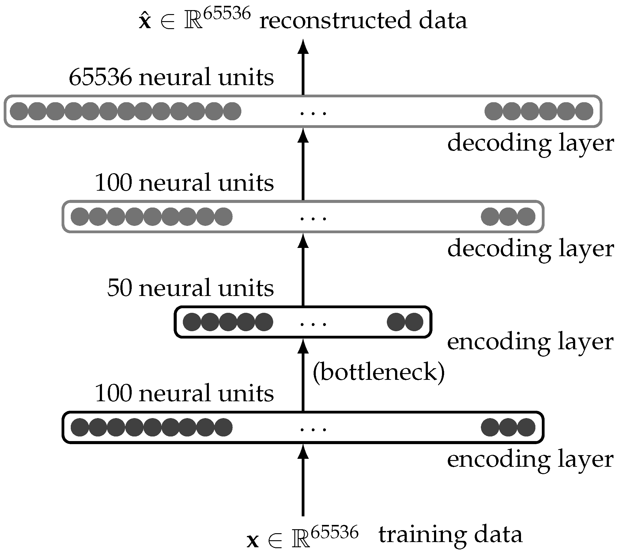
Autoencoders (AEs) have been a cornerstone in unsupervised learning, offering many applications ranging from dimensionality reduction to generative modeling [20]. The architecture of a classic autoencoder, as depicted in Figure 1, is particularly effective in learning compressed representations of high-dimensional data, such as images of size $256\times 256$ that flatten to a one-dimensional vector, $\mathbf{x}\in {\mathbb{R}}^{65536}$ [21]. The bottleneck layer, usually with the fewest neural units, is the central point of information compression [22,23].

Figure 1. Autoencoder architecture example using fully connected (dense) layers. Flattened input data goes through a series of encoding and decoding layers. The bottleneck offers access to compressed information of the input data.

Autoencoders have been extended to various forms, including convolutional autoencoders (CAEs), which are particularly effective in handling image data [24,25]. CAEs are a subset of CNNs and are generally trained in an unsupervised manner to learn spatial hierarchies of features [26,27]. They have been instrumental in various applications, from image denoising to anomaly detection [28,29]. Recent advancements have also led to the development of more complex variants like variational autoencoders (VAEs) and denoising AEs, which have shown promise in generative modeling and robust feature learning, respectively [30,31].

Quantum machine learning, particularly quantum autoencoders, is an emerging field that aims to leverage the computational advantages of quantum mechanics. Preliminary studies suggest that quantum autoencoders can perform comparably to their classical counterparts but with the added benefit of computational efficiency [32,33]. In cybersecurity, specifically for the analysis of DDoS attacks, hive plots serve as a multi-dimensional data visualization tool.

Our work builds upon both classical and quantum autoencoding techniques, aiming to push the boundaries of what is computationally possible and efficient in unsupervised learning [34,35].

2.1. Convolutional Autoencoder

CAEs have been the subject of extensive research, especially for unsupervised learning tasks [36,37]. They are a specialized type of autoencoder designed to handle grid-structured input data, like images [38,39]. The architecture typically consists of convolutional layers, adept at learning spatial hierarchies of features [36,37]. The primary objective of a CAE is to learn a compressed yet rich representation of the input data [40,41]. This is achieved by minimizing a reconstruction loss function, usually through backpropagation and gradient descent.

CAEs have found successful applications across various domains. For instance, researchers have used CAEs in agriculture to detect anomalies in agricultural vehicles [41]. In the field of power systems, engineers employ CAEs to detect high-impedance faults [42]. Similarly, the textile industry utilizes CAEs for identifying defects in fabrics [43]. In medical imaging, experts apply CAEs to assess lung cancer in CT images [44] and to detect infant cries and pain [40].

Furthermore, CAEs have been combined with other techniques to enhance their performance. For instance, combining CAEs with variational autoencoders (VAEs) has been used for unsupervised image clustering [45]. Integrating CAEs with long short-term memory (LSTM) networks has been employed for fall detection from thermal camera data [46]. Additionally, CAEs have been used in motion synthesis and editing, where they learn a representation of character motion [47].

CAEs are a powerful tool for unsupervised learning tasks, particularly in handling grid-structured input data like images. They have been successfully applied in various domains, including agriculture, power systems, fabric defect detection, medical imaging, and motion synthesis. Combining CAEs with other techniques has expanded their capabilities and improved their performance in different applications.

2.2. Quanvolutional Autoencoder for Computer Vision

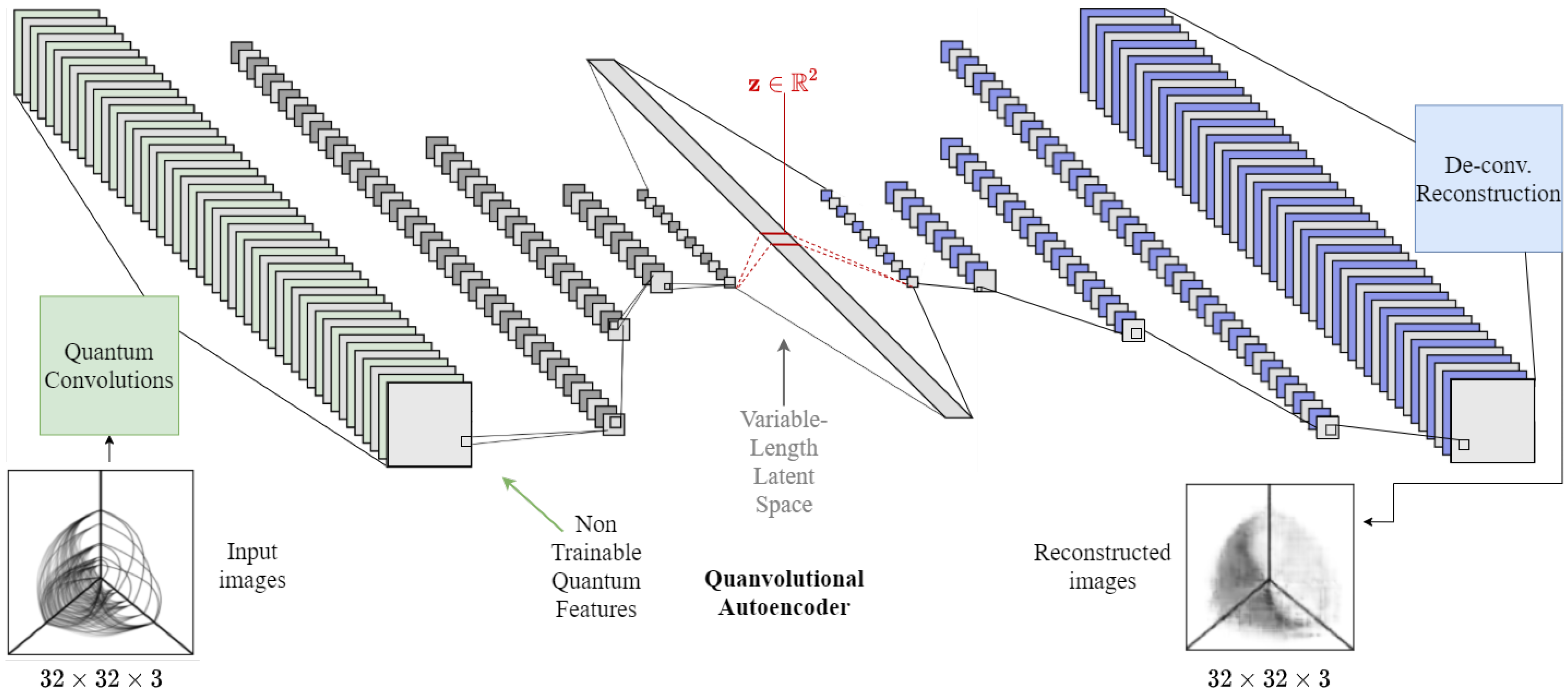
Quantum algorithms (QAs) hold great promise in the field of computer vision, offering rapid and secure information processing capabilities that are paramount for handling complex datasets. In this vein, we propose a novel architecture: a quanvolutional autoencoder (QAE), which combines the principles of quantum computing with the framework of a classical convolutional autoencoder to enhance feature learning and dimensionality reduction from image data. At the core of our approach is the replacement of conventional convolutional filters with quantum convolutions—a technique executed via a quantum circuit to perform feature extraction [48]. These quantum convolutions introduce a paradigm shift from classical processing, enabling the exploitation of quantum mechanical phenomena to handle the input data. Figure 2 depicts a streamlined view of the QAE architecture, delineating the progression from input to quanvolutional processing, subsequent encoding to a latent space, and final image reconstruction.

Figure 2. Generic architecture of a quanvolutional autoencoder. The quanvolutional layer initiates the feature extraction process from the input data. The encoder compresses these features into a dense latent space representation, $\mathbf{z}$, which is then expanded back to the original data structure by the decoder, culminating in the output.

Our interpretation of the QAE, while inspired by the original concept of quanvolutional neural networks [49], diverges significantly in both application and methodology. Unlike the classification focus of the prior work, our model is oriented towards unsupervised representation learning—a distinction that necessitates novel approaches to loss functions, layer design, and computational demands. Furthermore, our model is fully unsupervised and does not rely on labeled data, setting it apart from traditional supervised learning paradigms.

The efficacy of QAs in neural network architectures is partly constrained by the availability of qubits, which is a limitation more pronounced in physical implementations than in simulations. Despite this, the application of quantum information processing techniques to classical data represents a substantial advancement, harnessing both Gaussian and non-Gaussian quantum gates to achieve the linear and nonlinear transformations intrinsic to neural networks [50]. The adaptability of these quantum-based transformations to various data types has the potential to impact many areas, such as cybersecurity, which we will discuss next.

2.3. DDoS Attacks

In cybersecurity, a DDoS attack is a common type of organized attack. In particular, DDoS attacks are a common way to attack websites and other networked servers. These attacks are usually easy to perform and require little skill. The attack attempts to deplete a limited resource, such as server memory or CPU cycles, resulting in low service performance or significant delays in response time. Over the past year, the average DDoS attack size has increased by over 540%, with the maximum attack size exceeding a terabit/second. It is currently possible for unskilled attackers to rent botnets with about 500,000 connected devices. Such attacks are only expected to worsen since the number of minimally secured Internet of Things (IoT) devices that can be conscripted into botnets is expected to surpass 20 billion devices soon. DDoS attacks against organizations that use cloud services often cause bandwidth depletion and resource inaccessibility [51]. Thus, there is a significant need for new techniques that identify and mitigate DDoS attacks. In machine learning, DDoS detection and mitigation techniques can be addressed with machine learning algorithms [52,53,54,55]. Significant recent efforts include multi-channel CNNs for DDoS attack detection [56], multivariate regression analysis [57], and support vector machine-based techniques [58], to name a few. In this paper, we explore the novel approach of network traffic visualization using hive plots to investigate DDoS attacks.

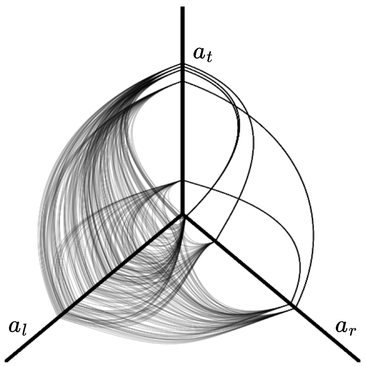
2.4. Introduction to Hive Plots

Attack pattern visualization is pivotal for extracting more meaningful information from complicated datasets. Researchers introduced hive plots as a straightforward approach to creating an informative, quantitative, and easily comparable depiction of multidimensional datasets [59,60,61,62]. Since then, hive plots have found applications in areas such as bioinformatics [61] and machine learning [53], to name a few. Hive plots are useful since they do not introduce artifacts like many other forms of data visualization. See Figure 3 as an example of a hive plot. In the figure, the example depicts a three-axis hive plot; for example, in a DDoS attack, these dimensions might represent the time of the attack, source IP address, and source country, which in the figure correspond to $a_l$, $a_r$, and $a_t$, respectively. The decision of which axis to use and how many axes to use depends on what we are trying to represent. This research will use hive plots to provide information about network traffic. This will enable us to study DDoS attacks from a QML perspective using convolutional AEs.

Figure 3. Example of a three-axis hive plot. Each axis $a_t$, $a_l$, and $a_r$ represents a dimension or information about the data. This example corresponds to a snapshot of network traffic; the top axis, $a_t$, represents the country of origin, the left axis, $a_l$, represents the time window, and the right axis, $a_r$, represents the source IP address; therefore, this example would be considered a DDoS attack pattern.

2.5. Quantum Autoencoder Implementation

Some tools can enable the implementation of a quantum autoencoder. The part that usually involves quantum computing operations is the execution of a quantum circuit. Qiskit is a language developed for quantum computing; it provides libraries, packages, and simulators with OpenQASM [63] and IBM-Q [64] quantum processors for implementing quantum circuits in a classical space. Deploying a feature_map function from the scikit-learn library has made quantum and classical data conversion possible, while IBM and QASM simulators provide a platform for developing a combination of quantum–classical applications. This research uses PennyLane libraries [65] that facilitate constructing a quantum circuit that can be executed in Qiskit or other similar platforms. PennyLane is a robust library, allowing for easy integration of quantum computing and machine learning platforms such as TensorFlow or PyTorch. Our research is based on TensorFlow and Qiskit through PennyLane.

2.6. Background on Quantum Computing

Quantum computing merges the principles of quantum physics with computer science, aiming to tackle specific problems that traditional computers find challenging. The quantum bit, or qubit, is a core element of quantum computing. It is capable of representing multiple states simultaneously through superposition, a feature distinct from the binary states of classical bits.

The unique capability of qubits to be in multiple states at once could theoretically enable quantum computers to solve particular problems much more efficiently than classical computers. Although the foundational concepts of quantum computing have been known for some time, it is only recently that practical quantum computers have started to become available. These devices are still in the early stages of capability, reminiscent of the early digital computers, and face significant limitations [66].

In the field of artificial intelligence and machine learning, quantum circuits are being explored for their potential to carry out classical computing tasks differently. Studies have shown that it is feasible to implement classical neural network algorithms, such as those used for training and evaluating neural networks, using quantum circuits [67]. This blending of classical and quantum computation is beginning to take shape in practical applications.

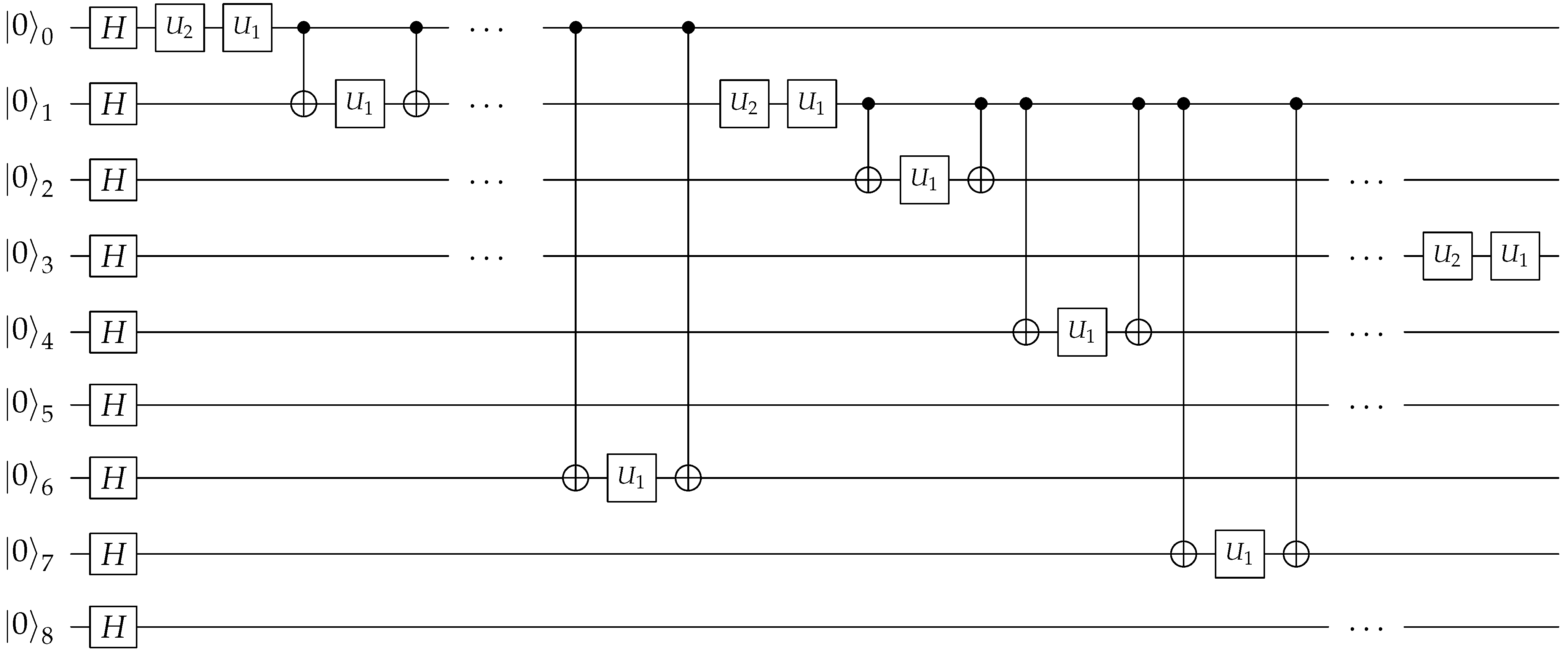
For example, researchers have designed quantum circuits that could streamline processes like k-fold cross-validation, a method widely used in machine learning, suggesting a quantum advantage in computational efficiency [68]. Our research contributes to this growing body of work by using a quantum circuit that incorporates a diverse array of quantum gates and operators. A segment of this circuit is shown in Figure 4 for illustrative purposes. The figure illustrates a 9-qubit portion of a larger 16-qubit circuit used in our experiments. It includes Hadamard gates, represented by H, and unitary operations, denoted by $U_i$. These operations, parameterizable by angles, are analogous to hyperparameters in classical machine learning [34]. Additionally, control and target qubits, represented by • and ⊕ symbols, respectively, are critical for the functioning of quantum gates and the subsequent manipulation of qubit states.

Figure 4. A sample 9-qubit quantum circuit with a quantum adiabatic algorithm that randomly implements different qubit operators. Note that our circuit uses 16 qubits with similar arbitrary placement of qubit operators to resemble and implement a quantum convolutional filter. Circuit drawn using the tool in [69].

The work of Shiba et al. also touches on this concept, employing a 9-qubit circuit for an autoencoder application [49]. Our research differentiates itself by exploring the use of random rotations to generate quantum convolutions, aiming to achieve efficient learning convergence and effective representation of data and matching or surpassing classical convolutional methods in performance. The specifics of our approach and its results will be detailed in Section 3.

2.7. Critical Review of the Existing Literature

The field of quantum machine learning has seen a surge in interest, particularly in the development of quantum autoencoders [24]. While these works have laid the foundation for quantum-based machine learning models, they often fall short in several key areas.

Firstly, the scalability of quantum autoencoders remains a significant concern. Most existing models are constrained by the number of qubits available, limiting their applicability to more complex datasets [24]. Secondly, the focus has primarily been on computational efficiency, often overlooking the model’s performance in real-world applications.

In the realm of classical autoencoders, particularly convolutional autoencoders, the literature is abundant but often lacks a focus on cybersecurity applications. While these classical models have been applied in various domains, their potential in cybersecurity, specifically in DDoS attack analysis, still needs to be explored [26].

Significantly, the existing literature on DDoS attacks primarily relies on classical machine learning algorithms, with little exploration into the potential of quantum machine learning [26]. This gap in understanding highlights the potential for quantum algorithms to revolutionize cybersecurity measures.

Our work introduces a novel concept in the field of quantum machine learning—the quanvolutional autoencoder. This model leverages the computational advantages of quantum mechanics and demonstrates its practical applicability in the realm of cybersecurity.

3. Methodology

Our central hypothesis is that a quanvolutional autoencoder can perform at the same level of accuracy as a traditional autoencoder but with faster convergence, using DDoS data as a test case. The experimental procedure we employed was designed to rigorously test our hypothesis. It is categorized into three parts: the first part discusses the dataset of hive plots, the second part describes the experimental setup, and the third part details the Qiskit implementation.

3.1. Hive Plots Dataset

For our experiments, we used a dataset comprising a large number of hive plots. In [53,54], the authors released a dataset that contains numerous instances of DDoS attacks and normal traffic represented using hive plots. Hive plots are frequently used for data visualization in big data mining. Simple visualization approaches such as bar charts and pie charts are generally ineffective for data depiction in the realm of big data mining [60]. For example, a hive plot can effectively illustrate computer networks and is a preferred method for data visualization and information communication. Unlike other network representation techniques like force diagrams, which do not always use a node coordinate system, hive plots organize nodes based on the structure of the network. These nodes are linked and positioned according to the network’s structural characteristics on radially arranged linear axes. Curved lines represent the edges connecting these nodes. Overall, hive plots are straightforward and easy to understand [60]. A hive plot can be constructed with multiple axes. The axes can represent the attributes of the data. The edges will be on the axes, which are linked with curves (Bezier curves), representing the relationships between the nodes. 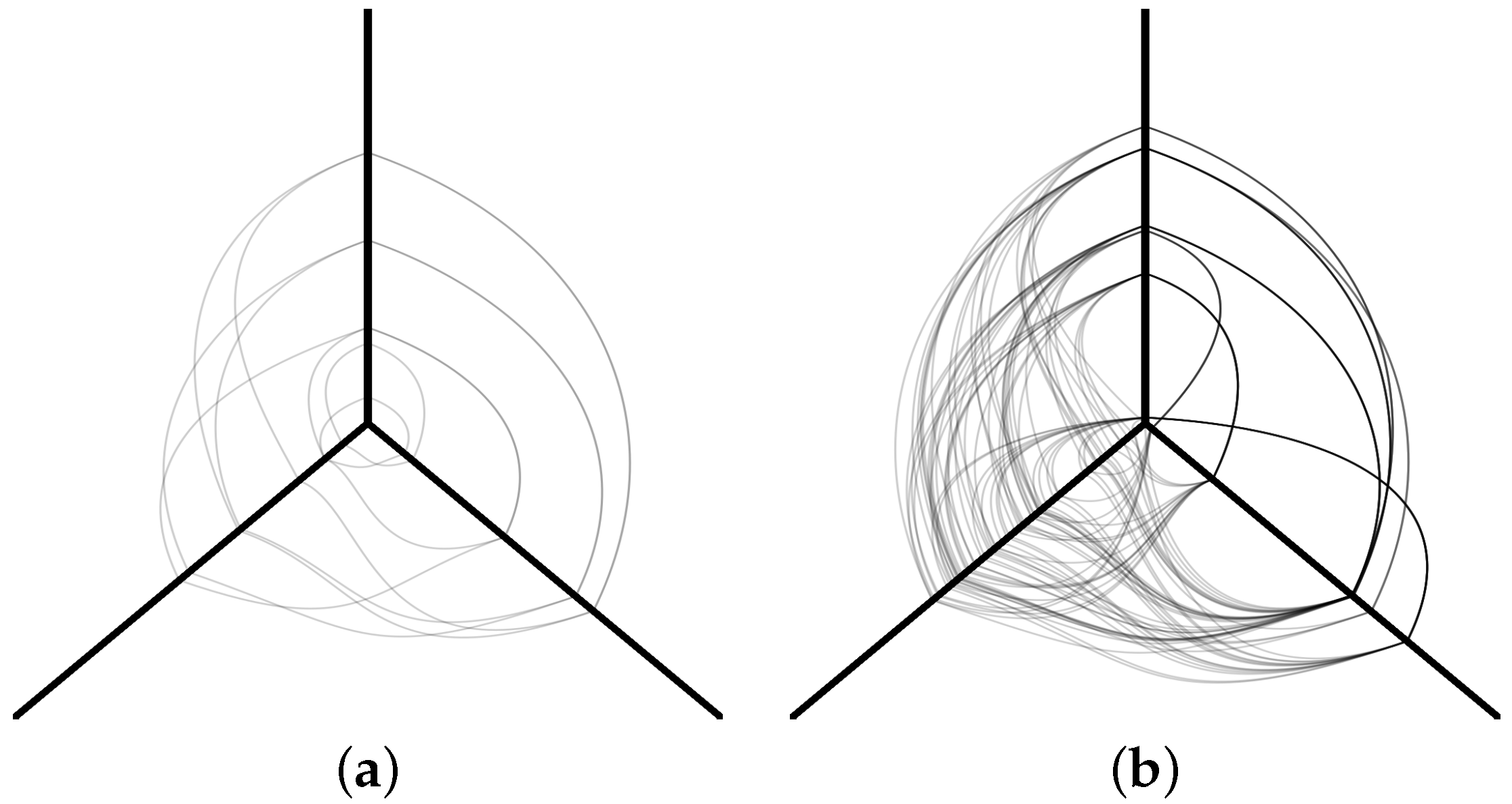Figure 5 depicts a sample hive plot diagram of three axes and multiple nodes and edges. The edges are the connections between nodes through the axes.

Figure 5. Example of a simple hive plot diagram from an experiment. (a) Normal traffic. (b) DDoS attack.

Figure 5a is a randomly selected sample from the hive plots corresponding to normal traffic, while Figure 5b depicts a DDoS attack hive plot. The figure has three axes: one going up, one right, and one left. The axis convention we followed was arbitrarily chosen as follows: the time in which the network traffic was recorded is shown on the left axis; the device’s source IP address is plotted on the right axis; and the country matching the source IP address is plotted on the top axis [53]. The hive plot dataset was built at Marist College by sending HTTPS requests in time steps into a honeypot called Peitho [53,54]. Randomization was used to simulate a real-world DDoS attack to determine the number of requests from each proxy to the honeypot. The attack data were received by submitting requests to an LCARS API (https://github.com/Marist-Innovation-Lab/LCARS, accessed on 14 February 2024). LCARS (Lightweight Cloud Application for Real-time Security) is an analysis and visualization tool used to perform graph analyses, hive plot visualizations, and relational analyses on collected log files of a honeynet [70]. LCARS aims to help explore correlations, frequencies, and outliers in cyberattack data.

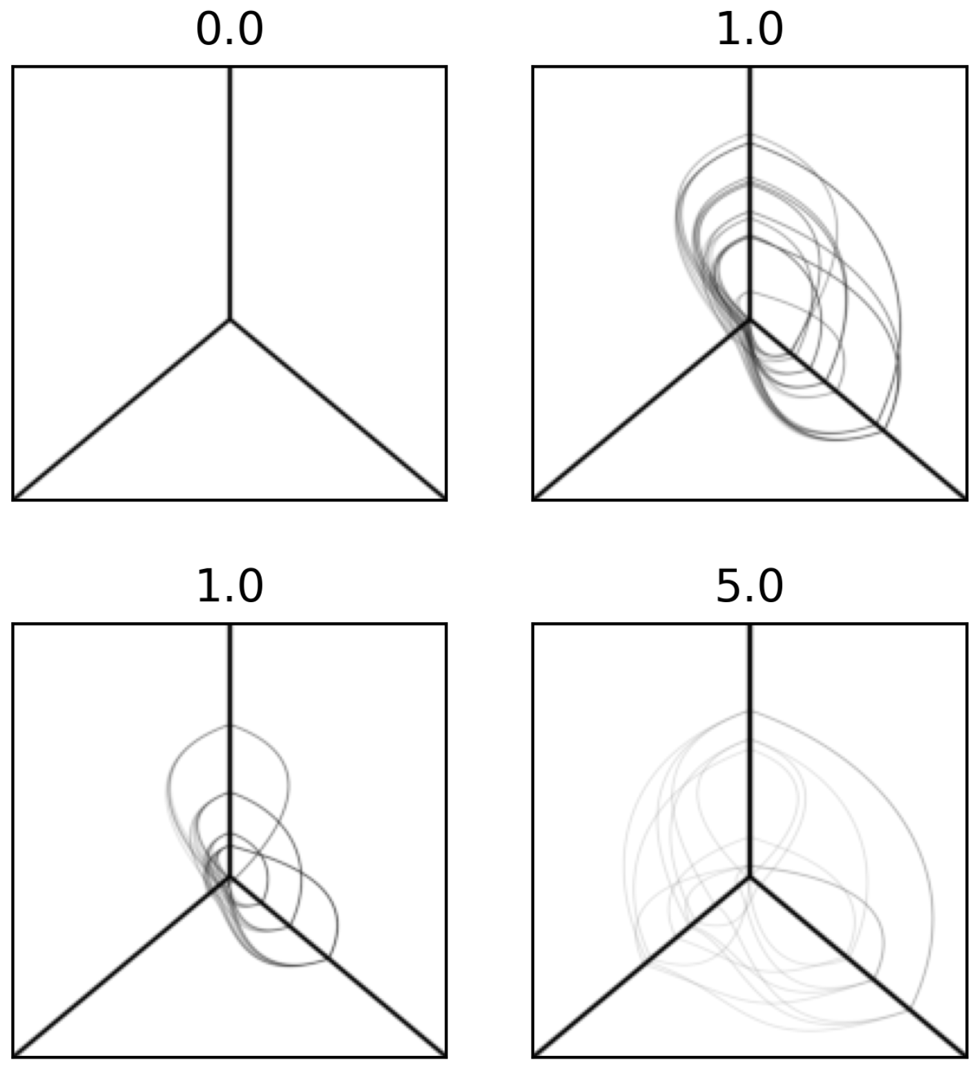
Using Python, one can display the hive plot along with information about the time sequence of the developing traffic for a specific time window; see Figure 6. The figure shows samples from the dataset taken at random from any sequence. The number at the top of the figure indicates the time step, which can vary from 0 to 7, which indicates the time step, t, in the sequence. The distance from the center represents a separation measure, e.g., the time gap between network traffic records. In Figure 6, the hive plot on the top left was taken at time step 0, and the hive plot on the top right was taken at time step 1. The bottom two figures are examples of different time steps, i.e., 1 and 5. Note that time step 0 is the same for all sequences, and it is used as a control group to make sure all such samples map to the same space induced by machine learning.

Figure 6. An example of hive plots from the hive plot dataset. The number on the top represents the time step. The three axes, top, left, and right, represent the country associated with the originating IP address, the number of times the service is requested, and the originating IP address, respectively. If fewer IP addresses from fewer countries are hitting more times, there is a possibility of DDoS attack formation, and if not, it represents a form of regular traffic.

From Figure 6 we can note on the top right that at time step 1 a DDoS attack is forming, as a small number of IP addresses and countries are hitting a significant number of times. The same description is true for the bottom left figure at time step 1. The bottom right hive plot, which is in time step 5, is an example of regular traffic, as several IP addresses and countries are hitting a minimal number of times.

3.2. Experimental Setup

We designed a simple autoencoder in a classical sense and another that takes advantage of quantum convolutions. The proposed quanvolutional (quantum convolutional) neural network architecture has a 16-qubit entanglement that acts as a receptive field, similar to the receptive field in the first layer of a CNN. The 16-qubits come from a $4\times 4$ window that acts as the CNN’s receptive field. A classic CNN learns filters (or matrices) that will be convolved with an input. CNN’s filters are learned using a gradient descent approach. A max-pooling procedure decreases the dimensionality of the results by taking the maximum of specific regions. Rectified linear unit (ReLU) activation functions are also used. In the middle of the classic autoencoder architecture, a bottleneck layer provides access to a latent space $\mathbf{z}\in {\mathbb{R}}^d$, after which the reconstruction process develops similarly. The process is repeated to construct the entire network with various filters at different sizes with the aforementioned traditional convolutional, pooling, deconvolutional, and upsampling layers.

Our proposed autoencoder for this experiment uses a set of non-trainable quantum-based filters, which are quantum circuits with entanglement. The classical version has 16 convolutional filters of size $9\times 9$, stride of $9\times 9$, and max pooling of size $3\times 3$ followed by ReLU. The next convolutional layer has 16 filters of size $3\times 3$ and stride $3\times 3$ followed by max pooling of size $2\times 2$ followed by ReLUs. The bottleneck has three dense layers of 512, 128, and 2 neural units. We are dressing the quantum version of this architecture with 16 qubits as a quanvolutional autoencoder. Figure 7 depicts our autoencoder architecture.

Figure 7. Convolutional neural network architecture for the hive plot experiment.

To train our model, we minimize a binary cross-entropy loss with the standard Adam optimizer with an initial learning rate of $0.001$ [71], and we stop the training after the model converges and has no improvement in the loss function for 15 epochs.

3.3. Python Implementation

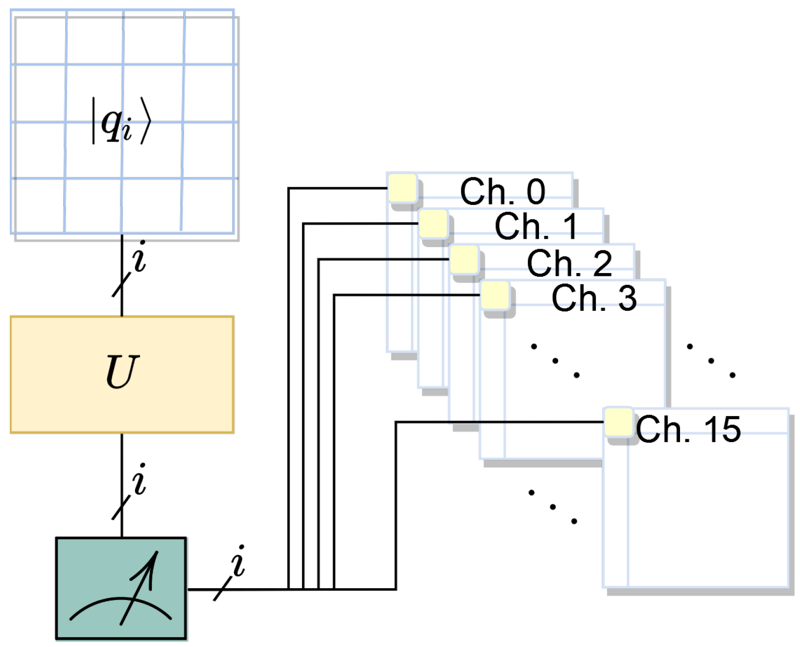
We employed the TensorFlow and Keras libraries to construct both the classical and quantum CNNs for our implementation. Our quanvolutional model leverages universal quantum circuits to process hive plots and extract spatial features for cyberattack analysis. The quantum circuit utilized in our model consists of 16 qubits with specific entanglement patterns, as depicted in Figure 8.

Figure 8. Diagram representing the quantum circuit used for quanvolution, featuring 16 qubits arranged in a $4\times 4$ grid. Each qubit is processed through the unitary operation U (refer to 1), and the outcome is measured and fed into one of 16 channels, denoted as Ch. 0 through Ch. 15. The notation $i=\{0,15\}$ specifies the index range of the qubits, indicating that each channel corresponds to the measurement of one qubit from the first (0) to the sixteenth (15). This configuration illustrates the mapping of a 16-qubit quantum state to a classical output, forming the basis for quantum-enhanced feature extraction.

Each qubit, denoted by $|q_i⟩$, corresponds to a spatial location in a $4\times 4$ grid, where $0\le i\le 15$. These qubits undergo a universal quantum gate operation U, defined as

$$\begin{array}{ccc}\hfill U& =& e^{i\alpha }{R}_{\widehat{n}}\left(\beta \right)R_{\widehat{m}}\left(\gamma \right)R_{\widehat{n}}\left(\delta \right).\hfill \end{array}$$

(1)

Here, $\alpha$ is a global phase, while $\beta ,\gamma ,\delta$ are rotation angles. The unit vectors $\widehat{m}$ and $\widehat{n}$ are non-parallel and define the axis of rotation. The operator $R_{\widehat{n}}\left(\theta \right)$ is a rotation matrix defined as $e^{-i\frac{\theta }{2}\widehat{n}·\overrightarrow{\sigma }}$, where $\overrightarrow{\sigma }$ represents the Pauli matrices [72].

The quantum circuit is parameterized by these angles and unit vectors, which are generally optimized during training. The optimization would usually be performed using gradient-based methods [35], and the backpropagation would be facilitated by parameter-shift rules specific to quantum circuits [73]. However, in our study, the circuits are non-trainable; instead, after the encoding described above, a randomized quantum circuit is applied, which consists of random layers generated by parameters drawn uniformly from the range $[0,2\pi )$. These layers include random rotations and entanglements acting on the qubits to process the encoded data. The random parameters for these layers are predetermined and remain fixed throughout the process, embodying the non-trainable aspect of our quantum model. The output of the quantum circuit is then measured, yielding expectation values with respect to the Z Pauli operator for each qubit. These values are interpreted as the processed features of the input patch and are utilized to construct the output feature maps of the quanvolutional layer.

This method allows for extracting complex spatial features from hive plots used in cyberattack analysis, leveraging the quantum mechanical properties of superposition and entanglement. Despite the non-trainable nature of the quantum circuits in our model, the random initialization of the circuit parameters facilitates a diverse and rich feature extraction mechanism distinct from conventional convolutional approaches.

To integrate the quantum layers into the classical CNN architecture, we used TensorFlow Quantum (TFQ), an extension of TensorFlow for hybrid quantum–classical machine learning. This allows seamless integration and enables the use of classical neural network layers alongside quantum layers.

The loss function used for training was binary cross-entropy, and the optimization was performed using the Adam optimizer with an initial learning rate of $0.001$ [71]. The training was halted if there was no improvement in the loss function for 15 consecutive epochs.

We refer to the specific steps outlined in Algorithm 1 for a comprehensive understanding of the proposed method.

Algorithm 1 Quanvolutional Autoencoder for DDoS Data Analysis

1: Input: Hive Plots Dataset   2: Output: Trained Quanvolutional Autoencoder Model                            ▹ Part 1: Hive Plots Dataset   3: Load the hive plots dataset [53,54]   4: Preprocess the dataset to fit the model architecture                            ▹ Part 2: Experimental Setup   5: Initialize classical and quantum autoencoder architectures   6: Set initial learning rate to $0.001$ [71]   7: Set loss function as binary cross-entropy   8: Set optimizer as Adam                          ▹ Part 3: Qiskit Implementation   9: Implement the 16-qubit quantum circuit as in Figure 8 10: Define the universal quantum operator U as in Equation (1)                                   ▹ Training 11: Train both classical and quantum models 12: Monitor the loss function for convergence 13: Stop training if no improvement for 15 epochs                                  ▹ Evaluation 14: Evaluate the models on test data 15: Compare the performance and convergence rate

3.4. Limitations of the Hive Plots Dataset

While extensive, the dataset used in this study is limited to hive plots generated from DDoS attacks and normal traffic. This specificity could introduce a bias in the model, making it less generalizable to other types of network traffic or cyberattacks. Additionally, the dataset was built at Marist College using a specific honeypot setup, which may not fully represent the diversity of real-world network configurations and DDoS attack strategies. Therefore, the results may only be universally applicable with further validation on more diverse datasets.

3.5. Computational Constraints and Non-Trainable Filters

The proposed quanvolutional autoencoder uses a 16-qubit entanglement, which, while innovative, introduces computational complexity that may not be easily scalable or practical for real-world applications at this time. Quantum computing resources are still nascent, and their availability is limited. Furthermore, the quantum-based filters in our architecture are non-trainable. This design choice was made to focus on the quantum advantages, but it also means that the model might need to adapt better to new or evolving types of DDoS attacks. The non-trainable nature of these filters could be a limitation regarding the model’s adaptability and long-term efficacy.

3.6. Unsupervised Nature and Class Separation in Quanvolutional Autoencoders

Autoencoders are inherently unsupervised learning models designed primarily for dimensionality reduction and feature learning. In the context of our research, the autoencoder is not used for classifying DDoS attacks from normal traffic; instead, it compresses the hive plot data into a lower-dimensional latent space. This latent space is then visualized to observe separations or clusters which could be labeled for classification.

It is important to note that while labels are used in the visualizations presented in this paper, the autoencoder model itself is not privy to these labels during the training phase. The labels are solely for the purpose of aiding human interpretation of the model’s performance and are not used as input or ground truth during the training process.

Furthermore, although autoencoders are not classifiers, they can be fine-tuned for classification tasks. One common approach is removing the autoencoder’s decoder portion and attaching a classification head to the bottleneck layer. However, this is beyond the scope of the current paper. Our primary focus is to demonstrate the potential of quanvolutional autoencoders in efficiently compressing and reconstructing hive plot data while showing through visual evidence that the compressed latent space could be helpful for classification tasks in future work.

4. Results and Discussion

Let us contrast the classical and quantum-based methodologies in a few different ways, including reconstruction ability, learned representations, and convergence.

4.1. Reconstruction Ability

Initially, we can look into the latent space induced by the autoencoder. An inspection of the latent space reveals the ability of the model to learn complex representations in low- and high-dimensional spaces. To vary the dimensionality of the latent space, we set the number of neurons in the intermediate dense layer, the “bottleneck”; see Figure 7 for reference. First, we set the bottleneck to encode down to 64 dimensions; second, the bottleneck encodes down to only 2 dimensions. This allows us to inspect the learned representations and observe their reconstruction abilities.

Figure 9 depicts the hive plot reconstructions achieved departing from latent spaces of 2 dimensions (a) and 64 dimensions (b). From the figure, we can visually observe slight differences in favor of better reconstructions using the high-dimensional representations. However, there are no significant differences from an information perspective; i.e., a trained human can still perceive whether a hive plot is an attack or regular traffic based solely on the reconstruction.

Figure 9. Classic convolutional autoencoder reconstructions from different latent space dimensions. (a) Reconstruction samples from 2 dimensions. (b) Reconstruction samples from 64 dimensions.

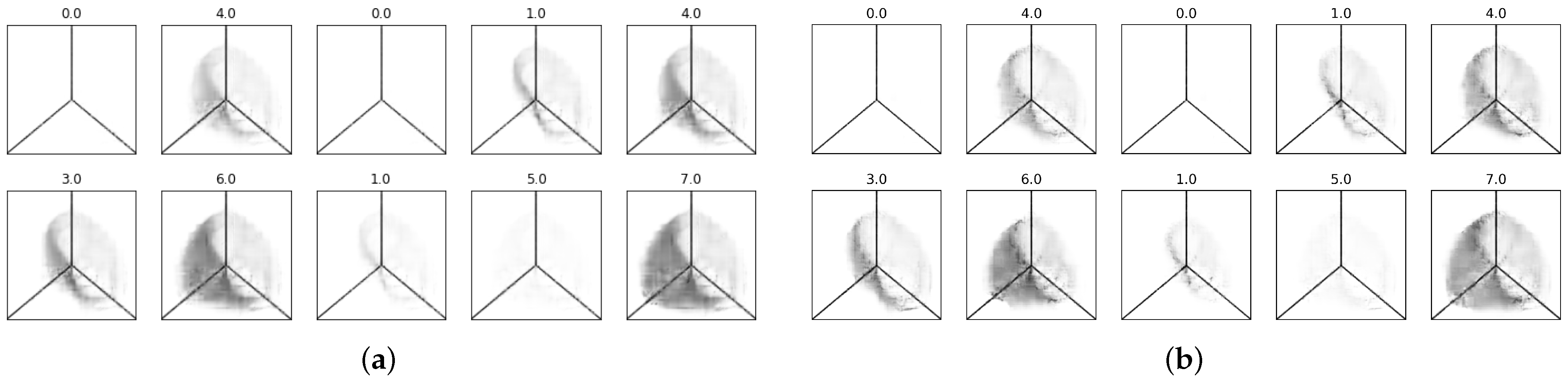
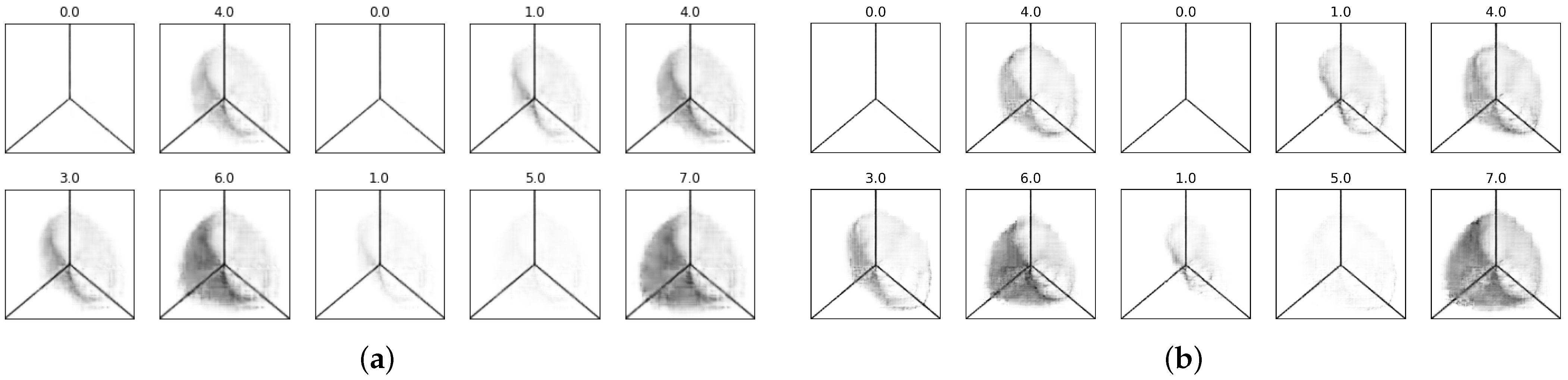
Similarly, Figure 10 shows the reconstructions obtained using our quanvolutional autoencoder model with both 2-dimensional (a) and 64-dimensional (b) latent space data. Both reconstructions look similar, although the one coming from the 64-dimensional space have more details. However, the important point is that a trained human can still distinguish whether a reconstructed sample represents normal traffic or a DDoS attack. For example, the right-most bottom two samples in Figure 10a,b are normal traffic and DDoS attacks, respectively.

Figure 10. Hive plots reconstructed with the quanvolutional autoencoder on latent spaces with different dimensions. (a) Reconstruction samples from 2 dimensions. (b) Reconstruction samples from 64 dimensions.

In comparison, both classic and quantum-based models exhibit similar reconstruction abilities; both can learn representations from hive plots. Based on the reconstructions learned down to different dimensions, visual inspection suggests similar reconstruction capabilities from a perceptual point of view. In particular, the reconstruction is thought to be optimal within the constraints given by the deep learning model itself, e.g., the information bottleneck and the loss function used, which are given by

$$\mathcal{L}(\theta ;\mathbf{x})=-\frac{1}{d}\sum _{i=1}^d{\mathbf{x}}_i·\log {\widehat{\mathbf{x}}}_i+\left(1-{\mathbf{x}}_i\right)·\log \left(1-{\widehat{\mathbf{x}}}_i\right),$$

(2)

where $\mathbf{x}\in {\mathbb{R}}^d$ is the input, $\widehat{\mathbf{x}}$ is the reconstruction, and $\theta$ are the model parameters. This is known as the binary cross-entropy loss. Minimizing this loss repeatedly, using random starts, yields consistent results across the board using the Adam optimizer with an initial learning rate of $0.0001$ and an automatic decay after a five-epoch plateau. The learning stops after no improvements in the validation loss after ten epochs.

4.2. Learned Representations

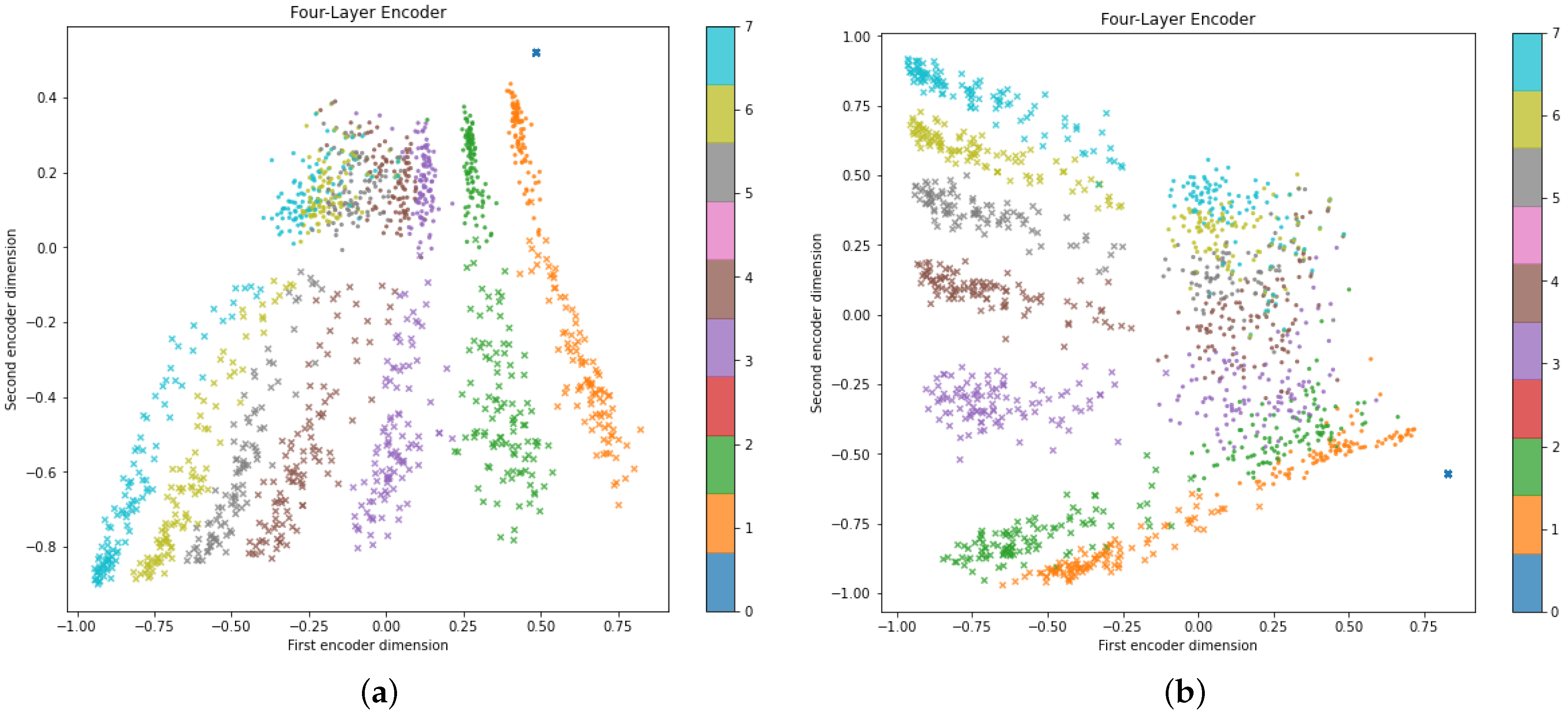
The next item to analyze is the learned latent space; this is arguably the most significant contribution of this paper. We begin by referring to Figure 11a, which shows every single hive plot on the dataset as a marker projected into a two-dimensional space induced by the autoencoder; dots (•) represent normal traffic, and crosses (×) represent the DDoS attacks, color-coded to show the stage of the attack. At time zero, all crosses and dots are in the same space on top of each other; both normal traffic and attack, since they are blank (no traffic) images of the axis, map to the same coordinates. This will serve as a “sanity check” to ensure the encoder is not learning spurious correlations among the input features.

Figure 11. Hive plot dataset compressed to a two-dimensional latent space using a classical and quanvolutional approach. (a) Learned representations with classic convolutional AE. (b) Learned representations with our quanvolutional AE.

Let us recall that the proposed autoencoder is not trained with any labels whatsoever. Yet, the model naturally makes two significant groupings: one group is lined up near the top, composed of normal traffic data (•); and the second group, DDoS attacks (×), are below the first group. This suggests that an autoencoder fine-tuned for binary classification could easily distinguish between regular traffic and an attack. The fine-tuning task is trivial, while the encoder–decoder design is novel. Furthermore, Figure 11a also indicates that eight different groups are also formed in different regions, each corresponding to the attack’s stage, t, and are indicated with different colors. These groups appear to be better differentiated, particularly when it comes to data representing attacks, while normal traffic data do not always form separate clusters for different time steps. Such a finding may also suggest that a fine-tuned autoencoder could determine whether an attack is happening and at which stage of development it is occurring.

Similarly, Figure 11b depicts the learned representations of the quanvolutional autoencoder. The learned space is very similar to a classic autoencoder; however, the dimensions induced by the encoder appear rotated in comparison. There are other minor differences concerning the separation between time steps, t, although overall, the results are comparable in performance. This suggests that the proposed autoencoder architecture is not degraded by replacing the convolutional feature maps at the input layer with quantum convolutional features.

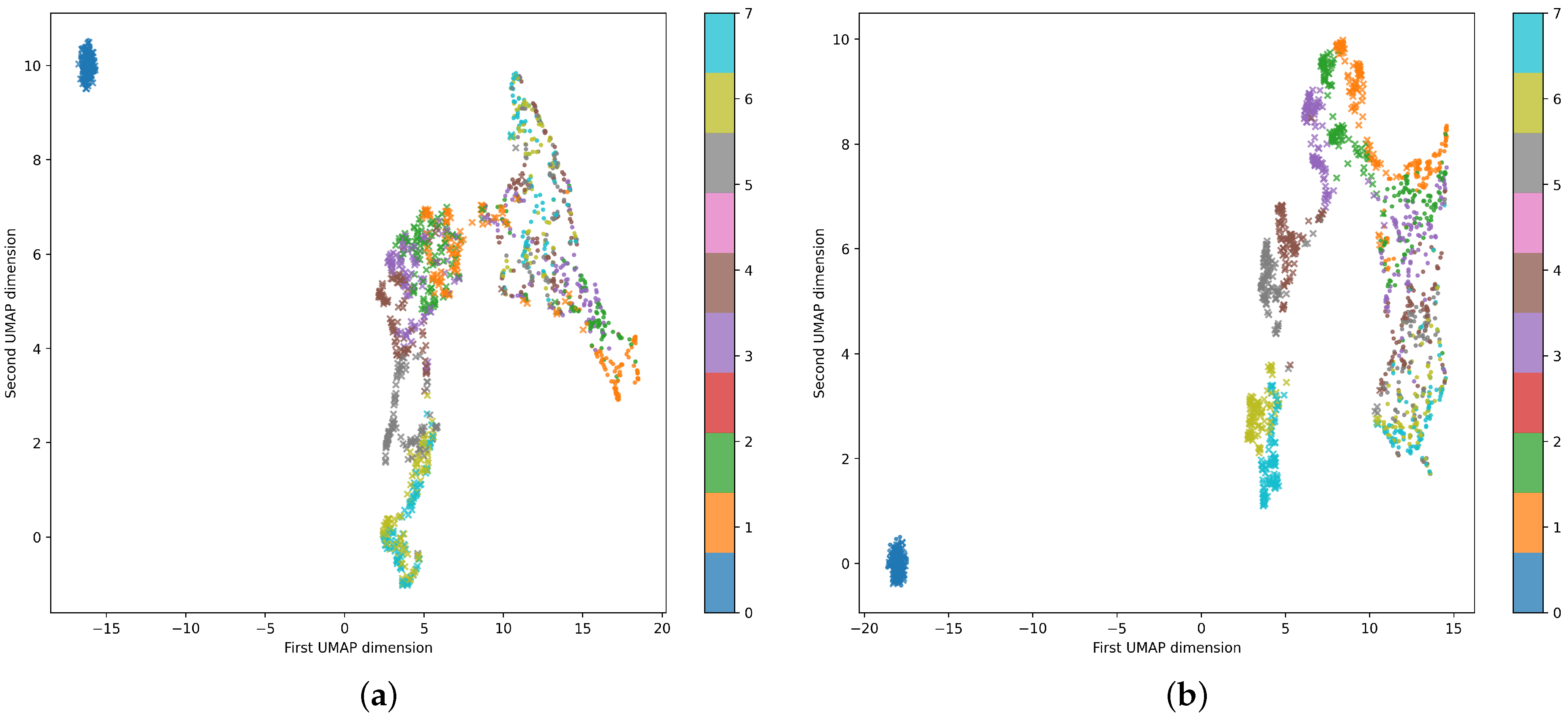
Similarly, Figure 12 focuses on analyzing the learned latent space using 64-dimensional data. The proposed autoencoder naturally divides the data into three major groups: no traffic (observed near the corner), normal traffic, and DDoS attacks. The model also differentiates between the different stages of an attack. The results of the quanvolutional autoencoder, Figure 12b, when compared with those of the classic autoencoder, Figure 12a, show that the proposed autoencoder architecture performs similarly and is not degraded by replacing the convolutional feature maps with quantum convolutional features. The plots in Figure 12 use UMAP to display 64-dimensional data in dimensions [74].

Figure 12. Comparison of the classification results from the quanvolutional and classical autoencoders with 64-dimensional data displayed in a two-dimensional plane using UMAP. (a) Classical neural network architecture on 64 dimensions. (b) Quanvolutional neural network architecture on 64 dimensions.

A more quantitative approach that demonstrates that our approach has a competitive advantage is discussed next in terms of convergence.

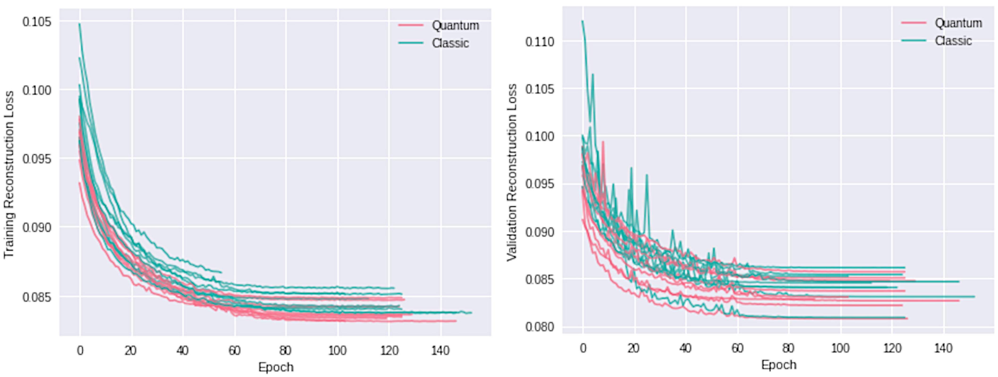
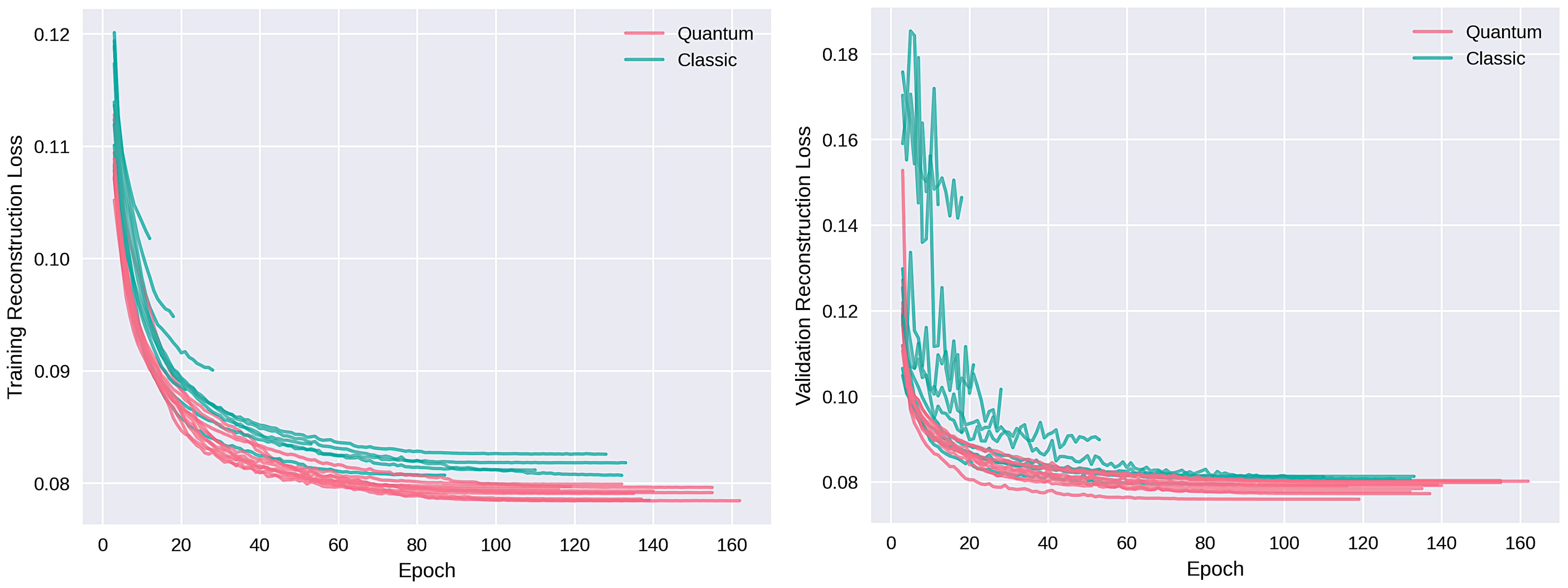
4.3. Convergence Efficiency

The loss in (2) is our function for evaluating convergence. Our quanvolutional autoencoder exhibits a promising decrease in loss, achieving final loss values comparable to the classical approach but within a notably shorter training span. Specifically, the quantum model attains equivalent loss levels 15 epochs earlier than its classical counterpart. In quantitative terms, if the classical model requires N epochs to converge, our quanvolutional autoencoder accomplishes a similar convergence by epoch $N-15$. This result is consistent across multiple runs with random initializations, as shown in Figure 13 and Figure 14 for two-dimensional data and for higher-dimensional data, respectively, which underscores the efficiency of our approach in rapid model fitting.

Figure 13. Losses for two-dimensional autoencoder. Left: Shows the training loss. Right: Shows the loss in validation data.

Figure 14. Losses for sixty-four-dimensional autoencoder. Left: Shows the training loss. Right: Shows the loss on validation data.

Training automatically terminates if no improvement in validation loss is observed for 50 consecutive epochs, enforcing a stringent criterion to prevent overfitting while also safeguarding against numerical instabilities commonly encountered in neural networks.

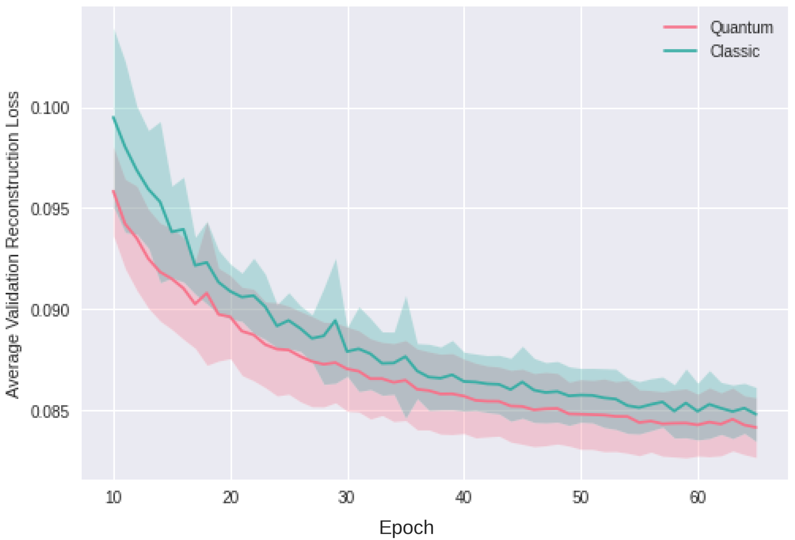
4.4. Learning Stability

The standard deviation of the loss function over distinct epoch intervals rigorously quantifies the stability of learning. During the initial 15 epochs, the quantum model demonstrates a stability index ($S_{1-15}$) of 0.06–0.10, reflecting 10 to 15 times greater stability compared to the classical approach, which has $S_{1-15}$ close to 1.0. This heightened stability is maintained in the 15–25 epoch interval, where the quantum model’s standard deviation is 10 to 5 times smaller ($S_{15-25}$), and continues to exhibit twice the stability ($S_{25-53}$ = 0.5) in the 25–53 epoch interval. 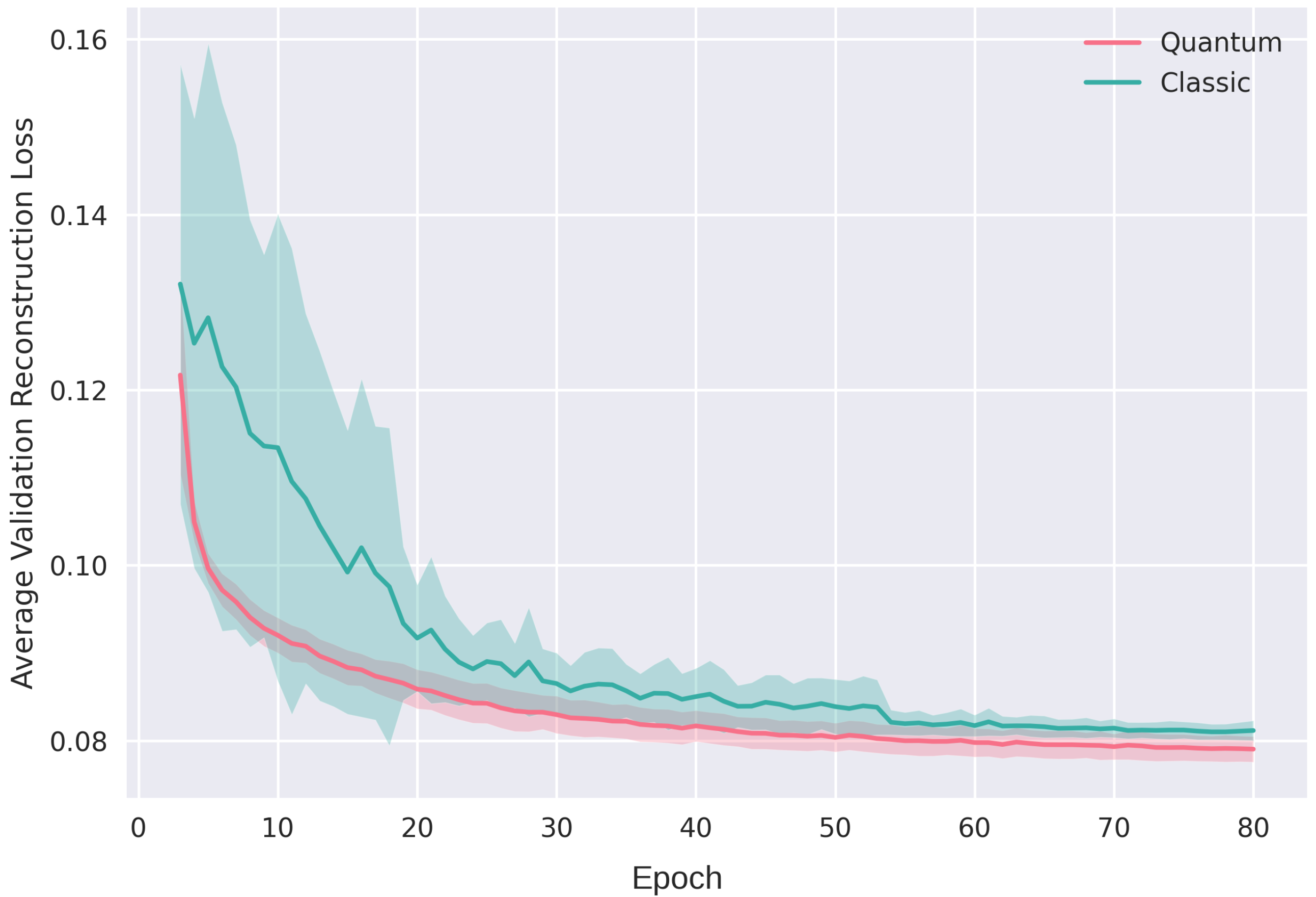Figure 15 and Figure 16 exclude initial outliers and concentrate on the epoch ranges indicative of most consistent performance, effectively visualizing the quantum model’s superior stability, particularly in handling 64-dimensional data challenges, validating its robustness in the gradient descent process.

Figure 15. Losses for validation of two-dimensional autoencoder.

Figure 16. Losses for validation of sixty-four-dimensional autoencoder.

4.5. Discussion on Scalability and Noise-Induced Barren Plateaus

As we explore the scalability of quantum autoencoders, with a specific focus on our proposed quanvolutional autoencoder, we must address not only the computational complexity but also the nuanced challenges introduced by quantum noise. Section 2.7 and Section 3.5 of our manuscript have already highlighted the dual hurdles of scaling computational complexity and managing noise in real-world applications. Here, we extend this discussion to incorporate the critical issue of noise-induced barren plateaus (NIBPs), as identified in recent research [75].

The computational complexity of quantum circuits, especially those leveraging entanglement and quanvolutional operations, is substantially influenced by the number of qubits, described as

$$C\left(n\right)={\alpha }_1·2^n+{\alpha }_2·n^2=\mathcal{O}\left(2^n\right),$$

(3)

where $C\left(n\right)$ denotes the computational complexity, n represents the number of qubits, and ${\alpha }_1$ and ${\alpha }_2$ quantify the base computational cost of quantum operations and the additional cost from entanglement and noise management, respectively. The exponential growth term, $2^n$, mirrors the expansion of the quantum state space, indicating a significant increase in computational complexity with larger qubit systems.

Crucially, the fidelity of quantum operations, a pivotal factor for the practical deployment of quantum algorithms, deteriorates with the system’s scale, as denoted by

$$F\left(n\right)=e^{-\gamma ·n},$$

(4)

where $F\left(n\right)$ signifies the operation’s fidelity and $\gamma$ represents the rate of decline in fidelity correlating with the increase in qubit count. This exponential decay highlights the challenge of preserving high-fidelity quantum operations in more extensive systems due to noise interference.

Incorporating insights from Wang et al. [75], we further understand that noise not only affects fidelity but also leads to NIBPs, where any kind of training associated with quantum algorithms becomes notably flat due to vanishing gradients, even if the circuit is not trainable, i.e., variational. This phenomenon grows exponentially more severe with the number of qubits, complicating the training of quantum and hybrid classic–quantum models on NISQ devices. For quantum circuits, particularly those with depths growing linearly with the number of qubits, the gradients can diminish exponentially, severely hindering the algorithm’s ability to learn and adapt the parameters of the circuit or model parameters surrounding the quantum circuit in the case of the dressed quantum model presented here. However, our model’s design, which incorporates non-learnable quanvolutional filters, is still susceptible to quantum noise interference but to a lesser degree, mitigating the risk of extreme detrimental effects arising from noise. Yet, at the current stage, expanding the system to include a larger number of qubits does not prove to be beneficial.

Addressing NIBPs and ensuring scalability requires innovative strategies beyond conventional error correction. Advanced error mitigation techniques and the development of noise-robust quantum algorithms emerge as essential for improving the practical viability and scalability of quantum autoencoders, including our quanvolutional autoencoder, for real-world applications. Our ongoing research, as detailed in [76], demonstrates a more resource-efficient approach to error mitigation by using a modified depolarizing channel, which reduces the reliance on complex matrix operations and avoids the use of the Pauli Y-gate. This approach enhances noise resilience and maintains a balance between circuit depth and computational efficiency. These findings currently guide our development of robust QML models and indicate potential extensions to multi-qubit systems for training more complex datasets. Future research will further explore these and other strategies, aiming to circumvent the limitations imposed by NIBPs and fully exploit the capabilities of quantum computing in complex domains.

5. Conclusions

This study contributes to the field of quantum machine learning by introducing the “quanvolutional autoencoder”, a novel architecture that leverages the computational advantages of quantum mechanics. The architecture was specifically designed to analyze time-series data from DDoS attacks, a critical issue in cybersecurity.

Our experimental results affirm that the quanvolutional autoencoder performs comparably to classical convolutional neural networks in visualizing and learning from DDoS hive plots. Notably, the quantum-based model demonstrated superior convergence rates and learning stability, as evidenced by Figure 13, Figure 14, Figure 15 and Figure 16. These findings validate the proposed model’s efficacy and highlight its potential advantages in real-world applications.

The intellectual merit of this work lies in its innovative fusion of quantum mechanics and machine learning algorithms. By employing a 16-qubit quantum convolutional neural network, the study pushes the boundaries of what is achievable with classical autoencoders, particularly in the context of cybersecurity.

However, it is crucial to acknowledge the limitations of this study. The dataset used is specific to hive plots generated from DDoS attacks, which may limit the model’s generalizability. Additionally, the computational complexity introduced by the 16-qubit entanglement and the non-trainable nature of the quantum filters could pose challenges in scalability and adaptability. These limitations suggest future research avenues, including exploring the model’s applicability to diverse datasets and its scalability in real-world scenarios.

This study is foundational for applying quantum machine learning in cybersecurity. It opens up new avenues for research, particularly in unsupervised anomaly detection, and sets the stage for future investigations that can build upon these initial findings.

References

- Chen, B.; Luo, W.; Luo, D. Identification of Audio Processing Operations Based on Convolutional Neural Network. In Proceedings of the 6th ACM Workshop on Information Hiding and Multimedia Security, New York, NY, USA, 20–22 June 2018; pp. 73–77. [Google Scholar] [CrossRef]
- Suganuma, M.; Kobayashi, M.; Shirakawa, S.; Nagao, T. Evolution of Deep Convolutional Neural Networks Using Cartesian Genetic Programming. Evol. Comput. 2020, 28, 141–163. [Google Scholar] [CrossRef] [PubMed]
- Suganuma, M.; Shirakawa, S.; Nagao, T. A Genetic Programming Approach to Designing Convolutional Neural Network Architectures. In Proceedings of the Genetic and Evolutionary Computation Conference, New York, NY, USA, 15–19 July 2017; pp. 497–504. [Google Scholar] [CrossRef]
- Kinnikar, A.; Husain, M.; Meena, S.M. Face Recognition Using Gabor Filter And Convolutional Neural Network. In Proceedings of the International Conference on Informatics and Analytics, New York, NY, USA, 25–26 August 2016. [Google Scholar] [CrossRef]
- Wang, H.; Tan, Y.; Liu, X.; Liu, N.; Chen, B. Face Recognition from Depth Images with Convolutional Neural Network. In Proceedings of the 2020 6th International Conference on Robotics and Artificial Intelligence, New York, NY, USA, 20–22 November 2020; pp. 15–18. [Google Scholar] [CrossRef]
- Chen, M.; Jiang, L.; Ma, C.; Sun, H. Bimodal Emotion Recognition Based on Convolutional Neural Network. In Proceedings of the 2019 11th International Conference on Machine Learning and Computing, New York, NY, USA, 22–24 February 2019; pp. 178–181. [Google Scholar] [CrossRef]
- Zhang, S.; Zhang, S.; Huang, T.; Gao, W. Multimodal Deep Convolutional Neural Network for Audio-Visual Emotion Recognition. In Proceedings of the 2016 ACM on International Conference on Multimedia Retrieval, New York, NY, USA, 6–9 June 2016; pp. 281–284. [Google Scholar] [CrossRef]
- Chen, M.; Shi, X.; Zhang, Y.; Wu, D.; Guizani, M. Deep features learning for medical image analysis with convolutional autoencoder neural network. IEEE Trans. Big Data 2017. [Google Scholar] [CrossRef]
- Ghasedi Dizaji, K.; Herandi, A.; Deng, C.; Cai, W.; Huang, H. Deep clustering via joint convolutional autoencoder embedding and relative entropy minimization. In Proceedings of the IEEE International Conference on Computer Vision, Venice, Italy, 22–29 October 2017; pp. 5736–5745. [Google Scholar]
- Biamonte, J.; Wittek, P.; Pancotti, N.; Rebentrost, P.; Wiebe, N.; Lloyd, S. Quantum machine learning. Nature 2017, 549, 195–202. [Google Scholar] [CrossRef] [PubMed]
- Schuld, M.; Sinayskiy, I.; Petruccione, F. An introduction to quantum machine learning. Contemp. Phys. 2015, 56, 172–185. [Google Scholar] [CrossRef]
- Gianani, I.; Mastroserio, I.; Buffoni, L.; Bruno, N.; Donati, L.; Cimini, V.; Barbieri, M.; Cataliotti, F.S.; Caruso, F. Experimental Quantum Embedding for Machine Learning. arXiv 2021, arXiv:2106.13835. [Google Scholar] [CrossRef]
- Schuld, M.; Killoran, N. Quantum machine learning in feature Hilbert spaces. Phys. Rev. Lett. 2019, 122, 040504. [Google Scholar] [CrossRef]
- Khanal, B.; Rivas, P. Evaluating the Impact of Noise on Variational Quantum Circuits in NISQ Era Devices. In Proceedings of the 2023 Congress in Computer Science, Computer Engineering, & Applied Computing (CSCE), Las Vegas, NV, USA, 24–27 July 2023; pp. 1–7. [Google Scholar]
- Khanal, B.; Orduz, J.; Rivas, P.; Baker, E.J. Supercomputing leverages quantum machine learning and grover’s algorithm. J. Supercomput. 2022, 79, 6918–6940. [Google Scholar] [CrossRef]
- Henderson, M.; Shakya, S.; Pradhan, S.; Cook, T. Quanvolutional neural networks: Powering image recognition with quantum circuits. Quantum Mach. Intell. 2020, 2, 2. [Google Scholar] [CrossRef]
- Mattern, D.; Martyniuk, D.; Willems, H.; Bergmann, F.; Paschke, A. Variational Quanvolutional Neural Networks with enhanced image encoding. arXiv 2021, arXiv:2106.07327. [Google Scholar]
- Tayba, M.N.; Maruf, A.A.; Rivas, P.; Baker, E.; Orduz, J. Using Quantum Circuits with Convolutional Neural Network for Pneumonia Detection. In Proceedings of the The Southwest Data Science Conference 2022, Waco, TX, USA, 25–26 March 2022; pp. 1–12. [Google Scholar]
- Suryotrisongko, H.; Musashi, Y.; Tsuneda, A.; Sugitani, K. Adversarial robustness in hybrid quantum-classical deep learning for botnet dga detection. J. Inf. Process. 2022, 30, 636–644. [Google Scholar] [CrossRef]
- Zeiler, M.D.; Fergus, R. Visualizing and understanding convolutional networks. In Proceedings of the Computer Vision–ECCV 2014: 13th European Conference, Zurich, Switzerland, 6–12 September 2014; Proceedings, Part I 13. Springer: Berlin/Heidelberg, Germany, 2014; pp. 818–833. [Google Scholar]
- Havlíček, V.; Córcoles, A.; Temme, K.; Harrow, A.; Kandala, A.; Chow, J.; Gambetta, J. Supervised learning with quantum-enhanced feature spaces. Nature 2019, 567, 209–212. [Google Scholar] [CrossRef] [PubMed]
- Akimoto, N.; Mitarai, K.; Leonardo, P.; Sugimoto, T.; Fujii, K. Vqe-generated quantum circuit dataset for machine learning. arXiv 2023, arXiv:2302.09751. [Google Scholar] [CrossRef]
- Mitarai, K.; Negoro, M.; Kitagawa, M.; Fujii, K. Quantum circuit learning. Phys. Rev. A 2018, 98, 032309. [Google Scholar] [CrossRef]
- Li, T.; Yao, Z.; Huang, X.; Zou, J.; Lin, T.; Li, W. Application of the quantum kernel algorithm on the particle identification at the besiii experiment. J. Phys. Conf. Ser. 2023, 2438, 012071. [Google Scholar] [CrossRef]
- Rebentrost, P.; Mohseni, M.; Lloyd, S. Quantum support vector machine for big data classification. Phys. Rev. Lett. 2014, 113, 130503. [Google Scholar] [CrossRef]
- Hou, S. Quantum lyapunov control with machine learning. Quantum Inf. Process. 2019, 19, 8. [Google Scholar] [CrossRef]
- Halladay, J.; Cullen, D.; Briner, N.; Warren, J.; Fye, K.; Basnet, R.; Bergen, J.; Doleck, T. Detection and characterization of ddos attacks using time-based features. IEEE Access 2022, 10, 49794–49807. [Google Scholar] [CrossRef]
- Blance, A.; Spannowsky, M. Quantum machine learning for particle physics using a variational quantum classifier. J. High Energy Phys. 2021, 2021, 212. [Google Scholar] [CrossRef]
- Zhang, C. Impact of defending strategy decision on ddos attack. Complexity 2021, 2021, 6694383. [Google Scholar] [CrossRef]
- Wei, Y.; Jang-Jaccard, J.; Sabrina, F.; Singh, A.; Xu, W.; Camtepe, S. Ae-mlp: A hybrid deep learning approach for ddos detection and classification. IEEE Access 2021, 9, 146810–146821. [Google Scholar] [CrossRef]
- Dong, S.; Sarem, M. Ddos attack detection method based on improved knn with the degree of ddos attack in software-defined networks. IEEE Access 2020, 8, 5039–5048. [Google Scholar] [CrossRef]
- Gyongyosi, L.; Imre, S. Optimizing high-efficiency quantum memory with quantum machine learning for near-term quantum devices. Sci. Rep. 2020, 10, 135. [Google Scholar] [CrossRef] [PubMed]
- Gao, J.; Qiao, L.; Jiao, Z.; Ma, Y.; Hu, C.; Ren, R.; Yang, A.; Tang, H.; Yung, M.; Jin, X. Experimental machine learning of quantum states. Phys. Rev. Lett. 2018, 120, 240501. [Google Scholar] [CrossRef] [PubMed]
- Rivas, P.; Zhao, L.; Orduz, J. Hybrid Quantum Variational Autoencoders for Representation Learning. In Proceedings of the 2021 International Conference on Computational Science and Computational Intelligence (CSCI), Las Vegas, NV, USA, 15–17 December 2021; pp. 52–57. [Google Scholar] [CrossRef]
- Rivas, P.; Zhao, L. On Unsupervised Reconstruction with Dressed Multilayered Variational Quantum Circuits. In Proceedings of the 2022 International Conference on Computational Science and Computational Intelligence (CSCI), Las Vegas, NV, USA, 14–16 December 2022; pp. 85–88. [Google Scholar] [CrossRef]
- Girshick, R.; Donahue, J.; Darrell, T.; Malik, J. Rich Feature Hierarchies for Accurate Object Detection and Semantic Segmentation. In Proceedings of the IEEE Conference on Computer Vision and Pattern Recognition (CVPR), Columbus, OH, USA, 23–28 June 2014. [Google Scholar] [CrossRef]
- Dai, J.; Qi, H.; Xiong, Y.; Li, Y.; Zhang, G.; Hu, H.; Wei, Y. Deformable Convolutional Networks. In Proceedings of the IEEE International Conference on Computer Vision (ICCV), Venice, Italy, 22–29 October 2017. [Google Scholar] [CrossRef]
- Carreira, J.; Zisserman, A. Quo Vadis, Action Recognition? A New Model and the Kinetics Dataset. In Proceedings of the IEEE Conference on Computer Vision and Pattern Recognition (CVPR), Honolulu, HI, USA, 21–26 July 2017. [Google Scholar] [CrossRef]
- Grais, E.M.; Plumbley, M.D. Single channel audio source separation using convolutional denoising autoencoders. In Proceedings of the 2017 IEEE Global Conference on Signal and Information Processing (GlobalSIP), Montreal, QC, Canada, 14–16 November 2017; pp. 1265–1269. [Google Scholar] [CrossRef]
- Kristian, Y.; Simogiarto, N.; Sampurna, M.; Hanindito, E.; Visuddho, V. Ensemble of multimodal deep learning autoencoder for infant cry and pain detection. F1000Research 2023, 11, 359. [Google Scholar] [CrossRef]
- Mujkic, E.; Philipsen, M.; Moeslund, T.; Christiansen, M.; Ravn, O. Anomaly detection for agricultural vehicles using autoencoders. Sensors 2022, 22, 3608. [Google Scholar] [CrossRef] [PubMed]
- Rai, K.; Hojatpanah, F.; Ajaei, F.; Grolinger, K. Deep learning for high-impedance fault detection: Convolutional autoencoders. Energies 2021, 14, 3623. [Google Scholar] [CrossRef]
- Han, Y.; Yu, H. Fabric defect detection system using stacked convolutional denoising auto-encoders trained with synthetic defect data. Appl. Sci. 2020, 10, 2511. [Google Scholar] [CrossRef]
- Silva, F.; Pereira, T.; Morgado, J.; Frade, J.; Mendes, J.; Freitas, C.; Negrão, E.; Lima, B.; Silva, M.; Madureira, A.; et al. EGFR assessment in lung cancer ct images: Analysis of local and holistic regions of interest using deep unsupervised transfer learning. IEEE Access 2021, 9, 58667–58676. [Google Scholar] [CrossRef]
- Chen, P.; Huang, J. A hybrid autoencoder network for unsupervised image clustering. Algorithms 2019, 12, 122. [Google Scholar] [CrossRef]
- Nogas, J.; Khan, S.S.; Mihailidis, A. Fall detection from thermal camera using convolutional lstm autoencoder. EasyChair Prepr. 2019. [Google Scholar] [CrossRef]
- Holden, D.; Saito, J.; Komura, T. A deep learning framework for character motion synthesis and editing. ACM Trans. Graph. 2016, 35, 1–11. [Google Scholar] [CrossRef]
- Sooksatra, K.; Rivas, P.; Orduz, J. Evaluating Accuracy and Adversarial Robustness of Quanvolutional Neural Networks. In Proceedings of the 2021 International Conference on Computational Science and Computational Intelligence (CSCI), Las Vegas, NV, USA, 15–17 December 2021; pp. 152–157. [Google Scholar] [CrossRef]
- Shiba, K.; Sakamoto, K.; Yamaguchi, K.; Malla, D.B.; Sogabe, T. Convolution filter embedded quantum gate autoencoder. arXiv 2019, arXiv:1906.01196. [Google Scholar]
- Killoran, N.; Bromley, T.R.; Arrazola, J.M.; Schuld, M.; Quesada, N.; Lloyd, S. Continuous-variable quantum neural networks. Phys. Rev. Res. 2019, 1, 033063. [Google Scholar] [CrossRef]
- Deshmukh, R.V.; Devadkar, K.K. Understanding DDoS attack & its effect in cloud environment. Procedia Comput. Sci. 2015, 49, 202–210. [Google Scholar]
- Villalobos, J.J.; Rodero, I.; Parashar, M. An Unsupervised Approach for Online Detection and Mitigation of High-Rate DDoS Attacks Based on an In-Memory Distributed Graph Using Streaming Data and Analytics. In Proceedings of the Fourth IEEE/ACM International Conference on Big Data Computing, Applications and Technologies, Austin, TX, USA, 5–8 December 2017; pp. 103–112. [Google Scholar] [CrossRef]
- Rivas, P.; DeCusatis, C.; Oakley, M.; Antaki, A.; Blaskey, N.; LaFalce, S.; Stone, S. Machine Learning for DDoS Attack Classification Using Hive Plots. In Proceedings of the 2019 IEEE 10th Annual Ubiquitous Computing, Electronics & Mobile Communication Conference (UEMCON), New York, NY, USA, 10–12 October 2019; pp. 0401–0407. [Google Scholar]
- Guarino, M.; Rivas, P.; DeCusatis, C. Towards Adversarially Robust DDoS-Attack Classification. In Proceedings of the 2020 11th IEEE Annual Ubiquitous Computing, Electronics & Mobile Communication Conference (UEMCON), New York, NY, USA, 28–31 October 2020; pp. 0285–0291. [Google Scholar]
- Huang, K.; Yang, L.; Yang, X.; Xiang, Y.; Tang, Y. A low-cost distributed denial-of-service attack architecture. IEEE Access 2020, 8, 42111–42119. [Google Scholar] [CrossRef]
- Chen, J.; Yang, Y.T.; Hu, K.K.; Zheng, H.B.; Wang, Z. DAD-MCNN: DDoS Attack Detection via Multi-channel CNN. In Proceedings of the 2019 11th International Conference on Machine Learning and Computing, Zhuhai, China, 22–24 February 2019; pp. 484–488. [Google Scholar] [CrossRef]
- Nagaraja, A.; Boregowda, U.; Vangipuram, R. Study of Detection of DDoS attacks in cloud environment Using Regression Analysis. In Proceedings of the International Conference on Data Science, E-learning and Information Systems 2021, Ma’an, Jordan, 5–7 April 2021; pp. 166–172. [Google Scholar] [CrossRef]
- Mehr, S.Y.; Ramamurthy, B. An SVM Based DDoS Attack Detection Method for Ryu SDN Controller. In Proceedings of the 15th International Conference on Emerging Networking Experiments and Technologies, Orlando, FL, USA, 9–12 December 2019; pp. 72–73. [Google Scholar] [CrossRef]
- Krzywinski, M.; Kasaian, K.; Morozova, O.; Birol, I.; Jones, S.J.M.; Marra, M. Linear Layout for Visualization of Networks. 2010. Available online: https://hiveplot.com/talks/hive-plot.pdf (accessed on 14 February 2024).
- Krzywinski, M.; Birol, I.; Jones, S.J.; Marra, M.A. Hive plots—Rational approach to visualizing networks. Brief. Bioinform. 2012, 13, 627–644. [Google Scholar] [CrossRef] [PubMed]
- Pocock, M.J.O.; Evans, D.M.; Fontaine, C.; Harvey, M.; Julliard, R.; McLaughlin, O.; Silvertown, J.; Tamaddoni-Nezhad, A.; White, P.C.L.; Bohan, D.A. Chapter Two-The Visualisation of Ecological Networks, and Their Use as a Tool for Engagement, Advocacy and Management. In Advances in Ecological Research; Woodward, G., Bohan, D.A., Eds.; Academic Press: Cambridge, MA, USA, 2016; Volume 54, pp. 41–85. [Google Scholar] [CrossRef]
- Engle, S.; Whalen, S. Visualizing distributed memory computations with hive plots. In Proceedings of the Ninth International Symposium on Visualization for Cyber Security-VizSec ’12, Seattle, WA, USA, 15 October 2012; pp. 56–63. [Google Scholar] [CrossRef]
- McKay, D.C.; Alexander, T.; Bello, L.; Biercuk, M.J.; Bishop, L.; Chen, J.; Chow, J.M.; Córcoles, A.D.; Egger, D.; Filipp, S.; et al. Qiskit backend specifications for openqasm and openpulse experiments. arXiv 2018, arXiv:1809.03452. [Google Scholar]
- Cross, A. The IBM Q experience and QISKit open-source quantum computing software. APS March Meet. Abstr. 2018, 2018, L58–003. [Google Scholar]
- Bergholm, V.; Izaac, J.; Schuld, M.; Gogolin, C.; Alam, M.S.; Ahmed, S.; Arrazola, J.M.; Blank, C.; Delgado, A.; Jahangiri, S.; et al. Pennylane: Automatic differentiation of hybrid quantum-classical computations. arXiv 2018, arXiv:1811.04968. [Google Scholar]
- Montanaro, A. Quantum algorithms: An overview. npj Quantum Inf. 2016, 2, 15023. [Google Scholar] [CrossRef]
- Allcock, J.; Hsieh, C.Y.; Kerenidis, I.; Zhang, S. Quantum Algorithms for Feedforward Neural Networks. ACM Trans. Quantum Comput. 2020, 1, 1–24. [Google Scholar] [CrossRef]
- dos Santos, P.G.; Araujo, I.C.; Sousa, R.S.; da Silva, A.J. Quantum Enhanced k-fold Cross-Validation. In Proceedings of the 2018 7th Brazilian Conference on Intelligent Systems (BRACIS), Sao Paulo, Brazil, 22–25 October 2018; pp. 194–199. [Google Scholar] [CrossRef]
- Eastin, B.; Flammia, S.T. Q-circuit tutorial. arXiv 2004, arXiv:quant-ph/0406003. [Google Scholar]
- Gisolfi, D.N.; Gutierrez, M.; Rimaldi, T.V.; DeCusatis, C.; Labouseur, A.G. A honeynet environment for analyzing malicious actors. In Proceedings of the 2018 IEEE MIT Undergraduate Research Technology Conference (URTC), Cambridge, MA, USA, 5–7 October 2018; pp. 1–5. [Google Scholar]
- Kingma, D.P.; Ba, J. Adam: A method for stochastic optimization. arXiv 2014, arXiv:1412.6980. [Google Scholar]
- Nielsen, M.A.; Chuang, I. Quantum Computation and Quantum Information; Cambridge University Press: Cambridge, UK, 2002. [Google Scholar]
- Cerezo, M.; Arrasmith, A.; Babbush, R.; Benjamin, S.C.; Endo, S.; Fujii, K.; McClean, J.R.; Mitarai, K.; Yuan, X.; Cincio, L.; et al. Variational quantum algorithms. Nat. Rev. Phys. 2021, 3, 625–644. [Google Scholar] [CrossRef]
- McInnes, L.; Healy, J.; Melville, J. Umap: Uniform manifold approximation and projection for dimension reduction. arXiv 2018, arXiv:1802.03426. [Google Scholar]
- Wang, S.; Fontana, E.; Cerezo, M.; Sharma, K.; Sone, A.; Cincio, L.; Coles, P.J. Noise-Induced Barren Plateaus in Variational Quantum Algorithms. Nat. Commun. 2021, 12, 6961. [Google Scholar] [CrossRef]
- Khanal, B.; Rivas, P. A Modified Depolarization Approach for Efficient Quantum Machine Learning. arXiv 2024, arXiv:2404.07330. [Google Scholar]
Figure 1.
Autoencoder architecture example using fully connected (dense) layers. Flattened input data goes through a series of encoding and decoding layers. The bottleneck offers access to compressed information of the input data.
Figure 2.
Generic architecture of a quanvolutional autoencoder. The quanvolutional layer initiates the feature extraction process from the input data. The encoder compresses these features into a dense latent space representation, , which is then expanded back to the original data structure by the decoder, culminating in the output.
Figure 3.
Example of a three-axis hive plot. Each axis , , and represents a dimension or information about the data. This example corresponds to a snapshot of network traffic; the top axis, , represents the country of origin, the left axis, , represents the time window, and the right axis, , represents the source IP address; therefore, this example would be considered a DDoS attack pattern.
Figure 4.
A sample 9-qubit quantum circuit with a quantum adiabatic algorithm that randomly implements different qubit operators. Note that our circuit uses 16 qubits with similar arbitrary placement of qubit operators to resemble and implement a quantum convolutional filter. Circuit drawn using the tool in [
69].
Figure 5.
Example of a simple hive plot diagram from an experiment. (a) Normal traffic. (b) DDoS attack.
Figure 6.
An example of hive plots from the hive plot dataset. The number on the top represents the time step. The three axes, top, left, and right, represent the country associated with the originating IP address, the number of times the service is requested, and the originating IP address, respectively. If fewer IP addresses from fewer countries are hitting more times, there is a possibility of DDoS attack formation, and if not, it represents a form of regular traffic.
Figure 7.
Convolutional neural network architecture for the hive plot experiment.
Figure 8.
Diagram representing the quantum circuit used for quanvolution, featuring 16 qubits arranged in a
grid. Each qubit is processed through the unitary operation
U (refer to
1), and the outcome is measured and fed into one of 16 channels, denoted as Ch. 0 through Ch. 15. The notation
specifies the index range of the qubits, indicating that each channel corresponds to the measurement of one qubit from the first (0) to the sixteenth (15). This configuration illustrates the mapping of a 16-qubit quantum state to a classical output, forming the basis for quantum-enhanced feature extraction.
Figure 9.
Classic convolutional autoencoder reconstructions from different latent space dimensions. (a) Reconstruction samples from 2 dimensions. (b) Reconstruction samples from 64 dimensions.
Figure 10.
Hive plots reconstructed with the quanvolutional autoencoder on latent spaces with different dimensions. (a) Reconstruction samples from 2 dimensions. (b) Reconstruction samples from 64 dimensions.
Figure 11.
Hive plot dataset compressed to a two-dimensional latent space using a classical and quanvolutional approach. (a) Learned representations with classic convolutional AE. (b) Learned representations with our quanvolutional AE.
Figure 12.
Comparison of the classification results from the quanvolutional and classical autoencoders with 64-dimensional data displayed in a two-dimensional plane using UMAP. (a) Classical neural network architecture on 64 dimensions. (b) Quanvolutional neural network architecture on 64 dimensions.
Figure 13.
Losses for two-dimensional autoencoder. Left: Shows the training loss. Right: Shows the loss in validation data.
Figure 14.
Losses for sixty-four-dimensional autoencoder. Left: Shows the training loss. Right: Shows the loss on validation data.
Figure 15.
Losses for validation of two-dimensional autoencoder.
Figure 16.
Losses for validation of sixty-four-dimensional autoencoder.