Distributed Learning in the IoT–Edge–Cloud Continuum

Abstract

The goal of the IoT–Edge–Cloud Continuum approach is to distribute computation and data loads across multiple types of devices taking advantage of the different strengths of each, such as proximity to the data source, data access, or computing power, while mitigating potential weaknesses. Most current machine learning operations are currently concentrated on remote high-performance computing devices, such as the cloud, which leads to challenges related to latency, privacy, and other inefficiencies. Distributed learning approaches can address these issues by enabling the distribution of machine learning operations throughout the IoT–Edge–Cloud Continuum by incorporating Edge and even IoT layers into machine learning operations more directly. Approaches like transfer learning could help to transfer the knowledge from more performant IoT–Edge–Cloud Continuum layers to more resource-constrained devices, e.g., IoT. The implementation of these methods in machine learning operations, including the related data handling security and privacy approaches, is challenging and actively being researched. In this article the distributed learning and transfer learning domains are researched, focusing on security, robustness, and privacy aspects, and their potential usage in the IoT–Edge–Cloud Continuum, including research on tools to use for implementing these methods. To achieve this, we have reviewed 145 sources and described the relevant methods as well as their relevant attack vectors and provided suggestions on mitigation.

1. Introduction

The power of IoT devices has increased to the level of being able to run machine learning (ML) algorithms both for inference and training. This has enabled a paradigm shift in machine learning from “big data” to “small data”, leading to the need for new methods for the safety and privacy in such ML models. Typically, the data are gathered in a centralized cloud location, where one central entity is the main controller of the ML operations (MLOps); however, with the described paradigm shift, the data can be processed in a distributed manner across the IoT–Edge–Cloud Continuum (IECC), creating a more distributed environment by scattering the influence of the MLOps to many devices. The IECC comes with a different set of potential issues in security and privacy due to the fact that data are exchanged between IoT, edge, and cloud devices, which usually have asymmetric access to data and asymmetric resources for processing. This leads to direct trade-offs between privacy and performance. Distributed learning (DL) has been proposed as the method that increases the safety and privacy of the models in such scenarios. To help with bringing DL to IoT devices, transfer learning is used to port models, e.g., from the cloud to IoT devices. In this paper, a review of distributed learning approaches and tools is provided together with discussion and guidance for potential implementers, allowing them to make educated decisions when implementing DL in IECC. In addition, because of the distributed manner of the IECC environment’s underpinnings, we strive to provide the necessary information in order to emphasize the aggregation nature of such systems. For this reason, this article focuses on the IECC domain as a whole and a more in-depth dive into each specific layer (IoT, Edge, etc.) of the IECC is left for future works. However, certain aspects of each layer are described and have been looked into in relation to implementing DL into the IECC.

The rest of the paper is structured as follows. Section 2 describes the field of the IoT–Edge–Cloud Continuum and its future directions. Section 3 focuses on distributed learning and the research on the methods it includes—federated learning and split learning. Section 4 is devoted to the transfer learning method research. In Section 5, the description for combinations of the DL and TL methods is provided. Section 6 describes the attack vectors in the scope of the researched methods, e.g., DL and TL, and Section 7 provides information about the attack mitigation approaches. Section 8 focuses on the tools to use for implementing the DL and TL methods. Discussion and future directions are described in Section 9, followed by the conclusions.

Related Works

The IECC domain is quite spread out, while many articles define their research focus in this domain, they sometimes have different specifications and small deviations. For example, the concept of the IoT–Fog–Cloud continuum [1,2] largely focuses on the same aspects with some differences. Here, the middle part—the fog—is more closer to the cloud, whereas the edge would be closer to the IoT layers [1]. This has been researched by Moreschini et al. [1]. They created a systematic mapping study in order to clarify the definitions for the cloud continuum.

Five review articles [2,3,4,5,6] and three survey articles [7,8,9] were found that research similar aspects of the IECC. Kampars et al. [3] reviewed the application layer communication protocols that can be used for interconnecting the layers of the IECC. S-Julián et al. [4] provide a review of the necessary capabilities of cloud-edge nodes in order to reach a fully equipped autonomous system. In order to reach a clearer consensus about the meaning of the edge–cloud continuum, Khalyeyev et al. [5] reviewed and generalized existing research articles in the field of the edge–cloud continuum. They emphasize the features that are expected as well as the challenges related to real-world deployments. In the field of IoT–Fog–Cloud computing, Bittencourt et al. [2] reviewed the challenges of the organization and management of such systems. In addition, they analyzed the directions in which applications can benefit from this computing paradigm. In order to provide a taxonomy for orchestration in the cloud-to-things compute continuum, Ullah et al. [6] reviewed existing state-of-the-art research on orchestration in this field. In addition, they proposed a high-level conceptual framework of orchestration. To categorize the current state of resource management simulation in the cloud-to-thing continuum, Bendechache et al. [7] developed a survey for the evaluation of software tools that are used for finding the most suitable methods, algorithms, and specific simulation approaches. The survey article from Gkonis et al. [8] combined the current technological advancements of the IECC, focusing on challenges as well as identifying open issues and limitations. Oliveira et al. [9] researched the mobile device technologies that could support the development of Edge–Cloud continuum systems by analyzing their mobility, characteristics, and popularity.

None of the found review and survey articles focus on the distributed learning methods for the IECC. Some mention federated learning [4,5,8,9] and transfer learning [8] However, they do not deeply research the innate challenges and problems related to this direction, such as security and privacy enhancing methods for DL in relation to the IECC domain. For this reason, this article focuses exactly on this subject in relation to the IECC.

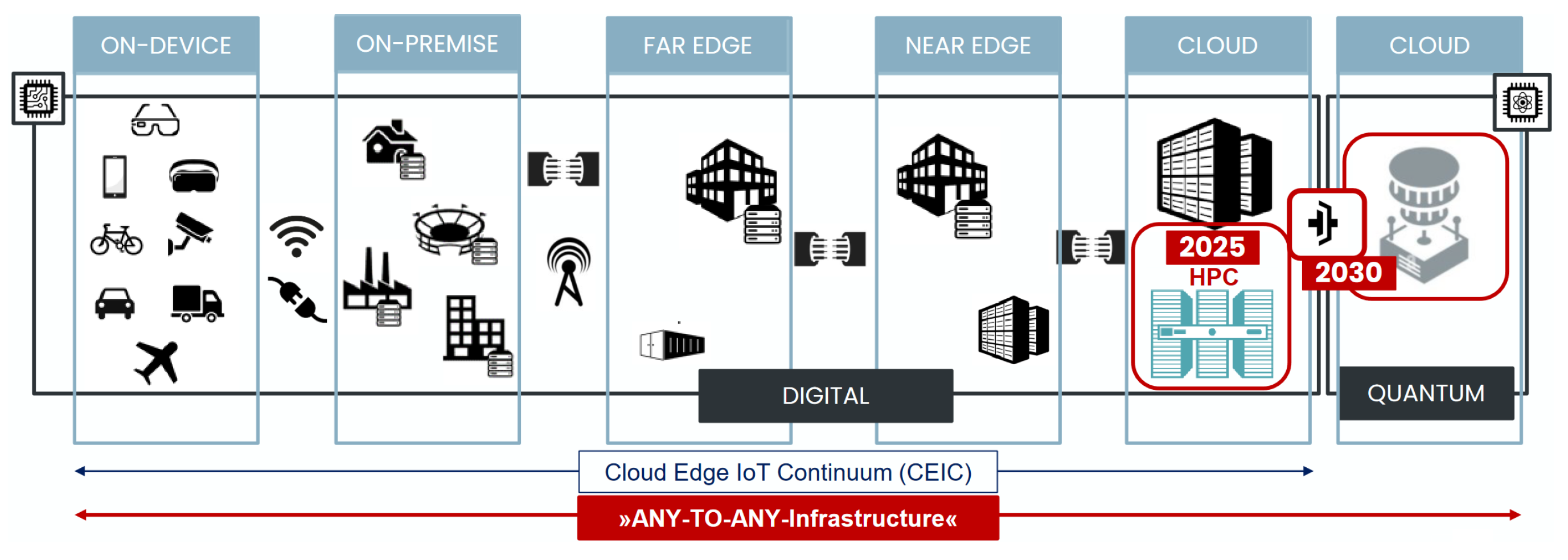
2. IoT–Edge–Cloud Continuum

One of the main goals of the IECC is to create a communication network where all layers—IoT, edge, and the Cloud—are indistinguishable and create one seamless continuum. In order to achieve a robust and smooth data path to the cloud, edge, and IoT devices [10]. To reach this goal, the research should be focused on a wide range of directions.

In Figure 1, current and future directions of the IECC are shown. As it is shown, the IECC could also be defined as the “Cloud Edge IoT Continuum”, which is essentially the same. We can see that the IECC starts at on-device deployments such as IoT devices or mobile phones and continues on on-premise venues, e.g., home server or PC, meaning the edge. These two layers may be connected through typical mediums, e.g., WiFi or LAN Ethernet. Further on, there are more edge layers using different long-distance connection types, for example, fiber optic cables or 4G/5G connections, until reaching the cloud, where high-performance clusters (HPC) may be used for high-performance computing tasks. In the future, quantum computing could be involved in this continuum [11]. All layers together create an any-to-any infrastructure. The idea is that any layer can be reached from any other layer, e.g., IoT-to-Cloud. Quantum computing could help in computational effectiveness as well as security but may also create problems related to post-quantum encryption resulting in certain encryption schemes being too vulnerable to quantum computing attacks. For this reason, practitioners should also think ahead and plan their security approaches to be safe against such computing power [12]. Further research related to quantum computing and security practices in this domain is out of the scope of this article.

The main challenge of implementing the IECC would be enforcing resilience, safety, security, and sovereignty (R3ST) using a system of systems, containing, for example, machine learning operations (MLOps) (see Figure 2), while concentrating on openness, such as the use of open-source tools. This article reviews the ways of overcoming this IECC challenge using distributed learning under the scope of MLOps, providing information about DL theory including security and privacy methods, as well as both open-source and proprietary tools available to implement DL methods. DL can help to solve the obstacles to IECC implementation. More specifically, DL tackles the obstacle of obtaining powerful-enough infrastructure performance for demanding workloads by distributing the computational burden throughout the continuum, incorporating as many layers as possible with optimal performance. This results in decentralized computing paradigms rather than a single central entity that does the main ML operations and that may become a bottleneck. Here, the whole continuum could be part of the MLOps computing task.

3. Distributed Learning

Li W. et al. [13] proposed a distribution diagram for machine learning on the Edge (see Figure 3). Here DL is part of the learning branch and splits into two methods—federated learning (FL) and split learning (SL).

Each DL approach was created to fix the shortcomings of the other method and to make ML operations more distributed and flexible to various hardware configurations and their distribution in multi-device networks. Other learning branch methods, e.g., transfer learning, are also frequently used in combination with DL methods because of the advantages this provides, specifically for devices with lower resources in comparison to the cloud infrastructure.

DL provides many ways to adapt to certain situations. In Figure 4, we can see three types of DL implementations. In (a), the classical method is described in which we have many local model training devices that send their results to a centralized entity—a cloud aggregation server. That will send the aggregated model back to each local device. The second method (b) works by utilizing only the Edge layer as the aggregation server. Here, local devices send their model results to the Edge aggregation server. That will send the aggregated results back. Lastly, the third method (c) describes a hierarchical model sometimes also called a cross-silo model [13,14,15]. Here, we have the Edge layer working as the intermediate aggregation server in which each Edge device has its own silo of local devices, e.g., hospitals or other facilities that send their data to this device for aggregation, but the Edge device sends the aggregated models to the cloud aggregation server to continue the aggregation process [13]. In this way, the computation process is more evenly distributed throughout the layers of the IECC—the aggregation is now hosted on both the cloud and the edge layers. The third approach increases the security from malicious activities from local clients because such clients could be filtered out in the edge layer and preventing the attack from reaching the main global model that is created in the cloud. From the privacy perspective, if the silos have homogeneous data, then we increase the privacy of the client model by increasing the size of the data; however, conversely, if we have heterogeneous data, we may stumble upon a problem of losing a great amount of model utility by the necessity of increasing privacy.

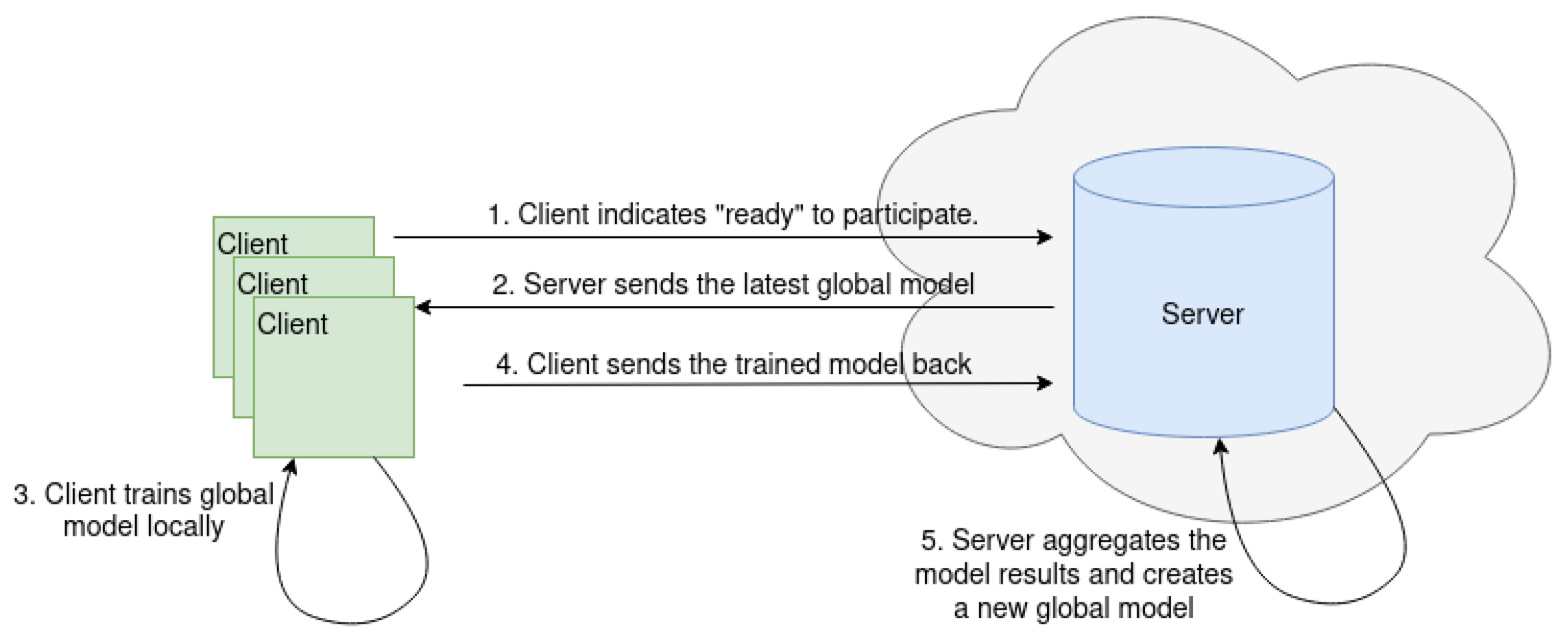
3.1. Federated Learning

The first reviewed DL method is federated learning (FL). Research in this domain is mostly concentrated on the proposed definition by Google (see Figure 5). This method is also sometimes called horizontal federated learning (HFL). Here, the assumption is that the clients share their feature spaces. However, that is not always the case. For this reason, vertical federated learning (VFL) was developed to tackle the difference in data feature space between clients [16]. Further analysis of the different FL directions can be found in [16] and is out of scope for this work.

The main idea of FL is to use ML algorithms on edge devices to increase data privacy and security by not letting each edge device’s data leave the data owner’s device. This can be accomplished by using privacy and security methods, e.g., differential privacy and secure aggregation. However, current research shows that whether or not the usage of FL implies the usage of the mentioned privacy and security methods is not strictly defined [17,18,19].

Federated learning allows us to train multiple ML model versions in parallel and to aggregate their results into one central model in order to reduce the necessary communication bandwidth by exchanging only the model results and not the initial data that the models are being trained on [19]. For example, let us imagine that our mobile phones are all part of the federated learning training network for a keyboard input recognition task. On each of our phones, a local model would be trained with our keyboard inputs to better recognize our writing style. Then, all or some of the models would be sent to the cloud for aggregation, resulting in a new global model. That is later sent to each mobile phone, replacing the local model to start another training round by training the newly received model [20].

This method can be deployed in many environments, such as, where the training process is synchronous or asynchronous. Let us take the synchronous example first. Figure 6 describes the synchronous FL model. After the client is ready to participate (step 1), the first step is for the client to send a request to join the training process to the server; (steps 2, 3) After the server has sent its global model, the client starts to train the model locally with the client’s local data; (step 4) If the server has chosen the client for the aggregation of the global model, the client sends the model results to the server for aggregation; and (step 5) After the server has aggregated the client model results, the training round starts over with step 1, if required—if the model has converged, the training need not continue [21,22].

By choosing to implement FL with the synchronous approach, certain clients may become a bottleneck and increase the training round time because of their inability to perform the training operations and send the model results fast enough. This may be the result of specific client-side or communication network problems such as less powerful computation resources in comparison to other edge devices. For example, if we have a federated learning network with multiple clients, their model download, local training, and upload times may differ, resulting in long waiting times in cases when some of the clients take longer than others. This brings to the fore the necessity for asynchronous aggregation of client model results [21,22].

John Nguyen et al. [22] created an FL asynchronous approach. The process of model download and training is the same as in the synchronous approach, but the model upload time limit is set. For this reason, clients who cannot upload their results in time are skipped and the aggregation procedure is executed without their results. However, the straggler results are still incorporated into the global model after they finish uploading them, to a certain degree determined by factoring in the delay of the upload.

In Figure 7, a comparison between asynchronous and synchronous federated learning is shown. We can see that in synchronous learning, denoted by SyncFL, the concurrent client count decreases drastically when the server has to wait for stragglers in each training round. However, if we look at the asynchronous approach, denoted by AsynchFL, we see that the concurrency at any given time t is almost equal throughout the training process. Furthermore, it is almost identical to the maximum achievable concurrency [22].

The aggregation of model results is actively being researched. There are many methods available. To name just a few:

• FedAvg—The default aggregating method that takes the average of received model results [23];
• FedProx—Improves the FedAvg method by adding regularization to optimize the aggregation results by limiting the differences between the local and global models. This method decreases the influence of result heterogeneity. Tian Li et al. [24] proposed this method and compared its effectiveness to FedAvg. The results showed that, in cases where there are no stragglers, both methods have essentially the same performance. However, by increasing the straggler count, the FedProx method beat FedAvg by a large margin. This was achieved by introducing a proximal term that defines the proximity of the local model in relation to the global model—this controls how far the local model can train away from the global model; thus, limiting the overfitting to the local model features. This results in the local model being closer to the global model. This problem may be the result of the local models having different local data features, dimensions, and other characteristics that make the model train further from other local models, including the global model. The FedProx method gets the best results because it uses the results from stragglers later on in the training process, and even uses their unfinished training results, while FedAvg just ignores them [24];
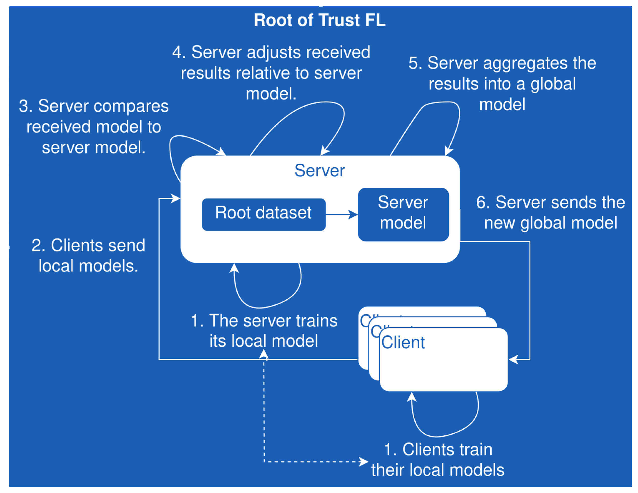
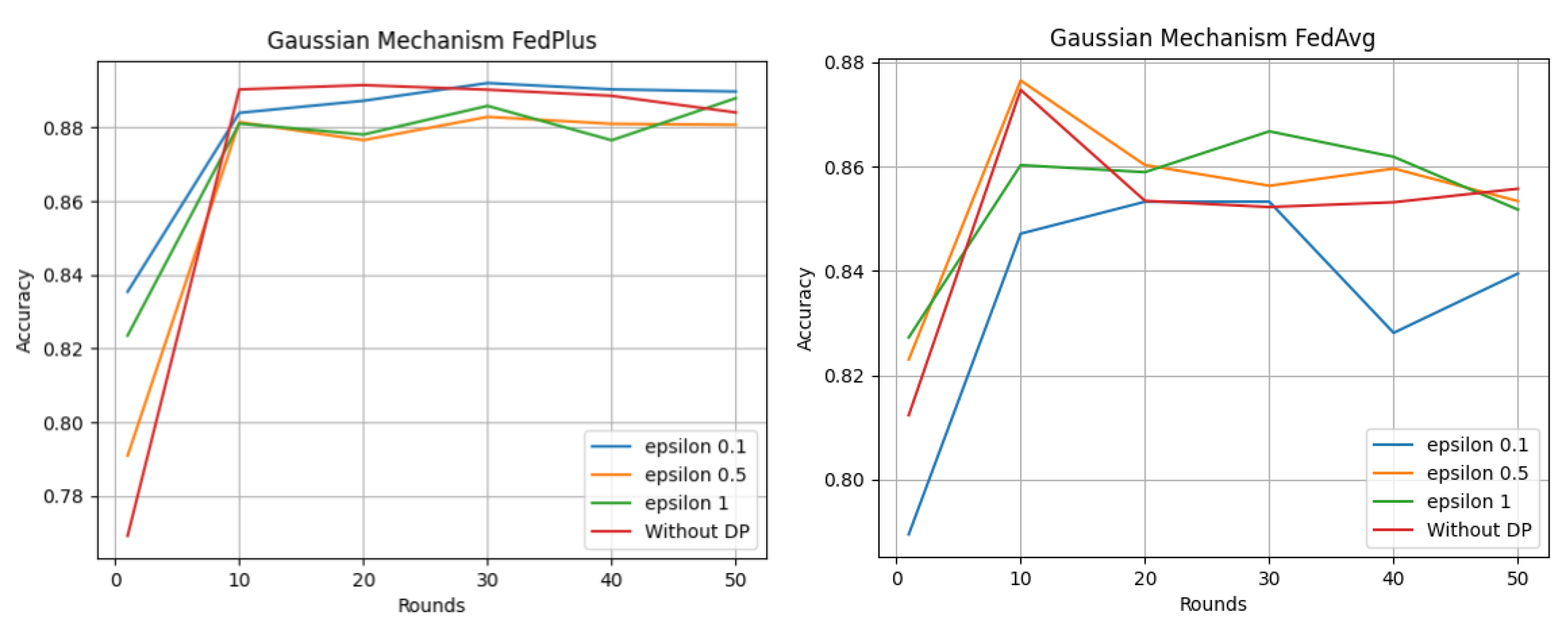
• Fed+—With this method, the clients have to start each training round with the local model gradients of the previous round. In this way, the local model features do not get lost after the aggregation step. This is why the usage of one global model is not required. This allows the aggregation to be organized in a hybrid manner—using Fel+ with other methods, e.g., FedAvg [25]. Pedro Ruzafa-Alcázar et al. [26] compared differential privacy approaches using two aggregation methods—Fed+ and FedAvg. In Figure 8, it can be seen that Fed+ reaches more stable and better results in comparison to the FedAvg method when the number of training rounds is increased. Epsilon denotes the privacy level of the training—the smaller the epsilon, the more private the training. The task of the models was to classify the intrusion type in IoT networks, e.g., DoS (Denial-of-Service) attacks using an open dataset;
• FedPAQ—Reisizadeh et al. [27] presented the method in which the aggregation rounds are created periodically, but the local model gradients are updated constantly. In order to decrease the delay that is created when the nodes are exchanging the model results and in order to make the model converge faster, client model results are quantized before sending them to the server. The authors analyzed the resulting training time for the new method by comparing it to the FedAvg approach. For all quantization levels that were used, the proposed approach allowed the model to converge faster in comparison to FedAvg;
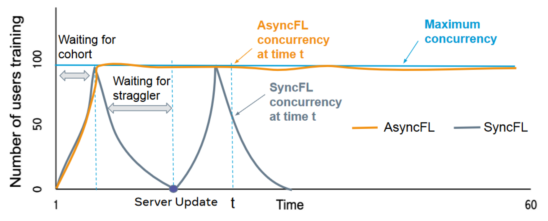
• FedBuff—This is an asynchronous FL aggregation method that aggregates the client gradients at the server with increased security by saving their gradients in a secure buffer, e.g., a trusted execution environment. In

  Table 1. Comparison between FedBuff and other methods [22].

  Dataset	Precision	FedBuff	FedAvg	FedProx
  CelebA	90%	31.9	231 (8.5x)	228 (8.4x)
  Sent140	69%	124.7	>600	>600
  CIFAR-10	60%	67.5	386.7 (5.7x)	292.7 (4.3x)

  , a performance comparison between FedBuff, FedAvg, and FedProx can be seen. Three datasets were used—CelebA, Send140, and CIFAR-10. The precision column shows the achievable precision for each dataset. The columns for aggregation methods describe the necessary communication time count between the clients and the server. One unit represents 1000 trips. Table 1 shows that with FedBuff, we obtain an approximately 8.5x speedup in comparison to other methods for CelebA, a 5.7x speedup in comparison to FedAvg, and a 4.3x speedup in comparison to FedProx for CIFAR-10. Lastly, FedBuff achieved the goal precision for Send140 with 124,700 communication trips, while FedAvg and FedProx did not manage to reach the goal precision in the predefined limit (600,000 times) [22].

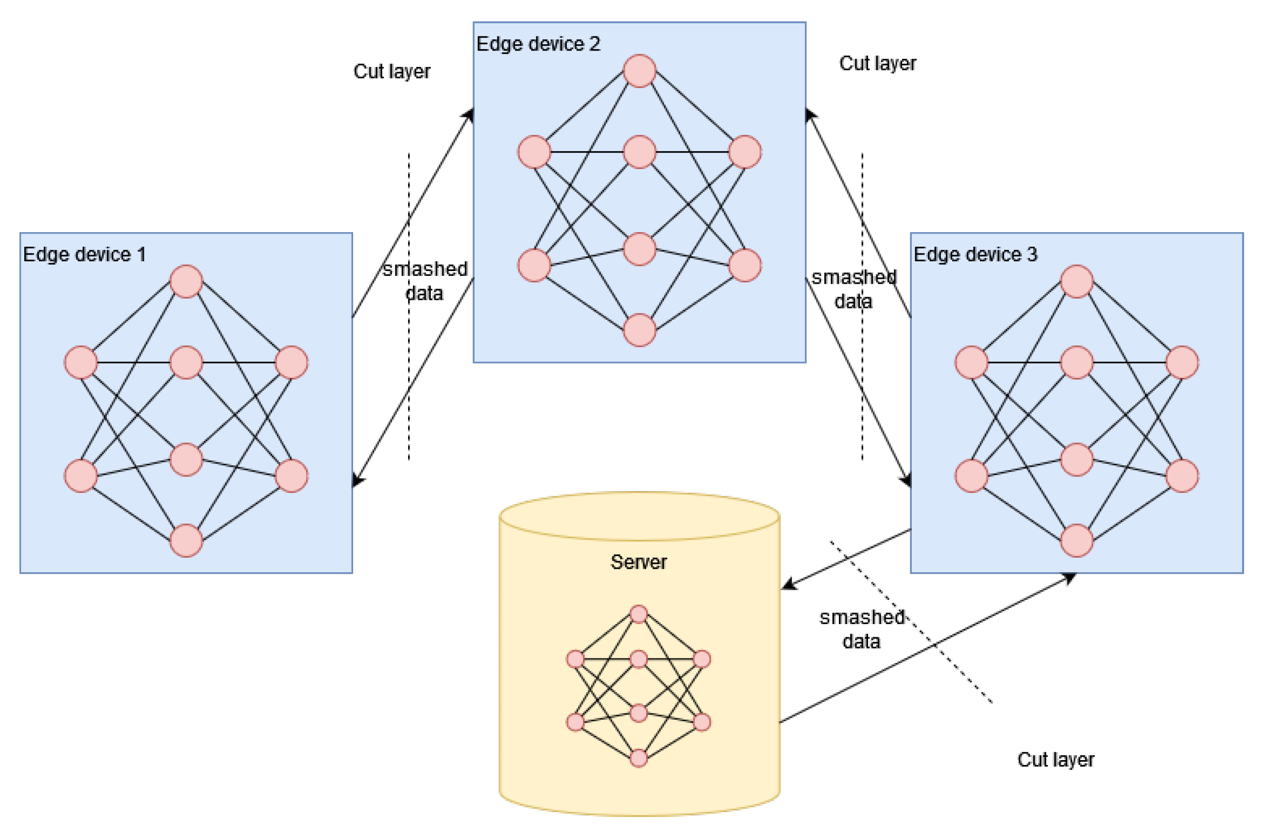
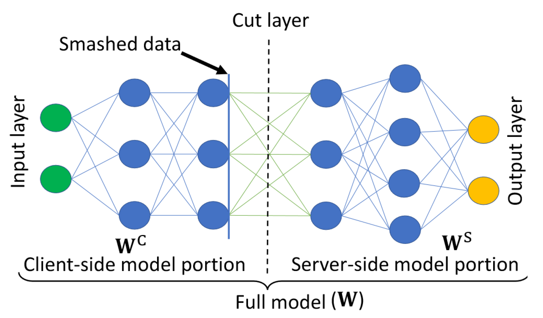
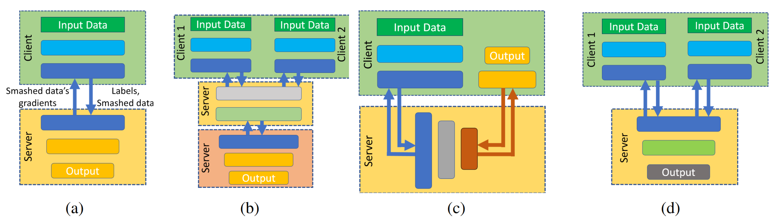
The above-mentioned methods represent only a small part of the existing aggregation methods. More detailed research on FL aggregation methods is out of the scope of this review article and would call for another review article concentrating on this specific purpose because of the sheer quantity of methods and the possibilities of the analysis directions. There are many more methods with more features, e.g., privacy and security aspects [13,24,28,29,30,31,32,33,34,35,36].

Federated learning increases the privacy of the data because the local input data do not leave the local device. Only the model results are sent onward, to the central server or other clients. That said, there are approaches with which one could possibly retrieve the input data or parts from them by utilizing only the model gradients using gradient inversion attacks. For example, if we have a model that is trained on image data, it could be possible to retrieve the initial input images or a specific image using this attack. This means that the model gradients still leak information about the initial input data [21]. Not only image data can be retrieved using this attack, even text can be retrieved. Ruisi Zhang et al. [37] showed how model inversion attacks can be used to reconstruct text input data from transformer models. However, model inversion produces the average of the features that, at best, can characterize an entire output class. It does not: (1) construct a specific member of the training dataset, or (2) give an input and a model, determining if this specific input was used to train the model [38]. Regardless, we need a method that could reduce the success rate of model inversion attacks. In addition, training the whole model on low-power devices, e.g., a Raspberry Pi, may not suffice in the age of large language models and transformers. That is why we need a method that allows us to distribute the computation more evenly in relation to the available resources of the devices in the network.

The FL method has been widely used. For example, Walskaar et al. [39] developed an FL implementation for COVID-19 X-ray lung scan data analysis. Liu et al. [40] created VFL and HFL frameworks for power consumption forecasting. Stripelis et al. [41] used FL for neuroimaging analysis. A wider analysis of the applications of FL can be seen in [42], in which Shaheen and co-authors present the wide range of directions in which the FL method has been applied. These include healthcare, autonomous vehicles, and finance [42].

3.2. Split Learning

In split learning, models are divided into two or more parts and scattered around the device network. All these devices combined will train one model in a sequential manner, relative to the way the model is distributed.

This method is the successor to federated learning; however, it has not yet gained much traction. Consequently, there are fewer available research articles regarding existing SL approaches, and privacy and security methods for SL, in comparison to the FL method.

In Figure 9, an example of SL is shown. Here, one model is divided into two parts. On the left-hand side, we have a client-side portion ($W_C$), which could be deployed, e.g., on your Raspberry Pi or other Edge or IoT device. On the right-hand side, we have the server-side portion ($W_S$), which could be deployed in the cloud. The part where the model is divided is called the Cut Layer, and the data that are distributed between the model parts are called smashed data. The training and inference process is sequential. In a forward propagation task, the client starts the propagation until the cut layer using the input data. The activations of the last layer (smashed data) are then sent to the server side. The server receives the smashed data as input data and continues the propagation. However, in backpropagation, after the calculation of the loss function, the server starts the propagation by calculating the gradients and the activation values for all layers until the cut layer. After that, the server sends the results (smashed data) to the client side, where the client continues the backpropagation [43].

There are various directions you could take to implement the split learning method. Figure 10 shows four such direction. Firstly, in (a) we can see the same configuration as that shown in Figure 9. The gradients and the labels are shared between two parts of the model, one of which is located on a client device and the other on a server. In (b), however, an intermediate node is used. This configuration reduces the computational load on the server by moving some layers from the server node to the intermediate node when the client device count is increased. You could think of this as the hierarchical model in DL (see Figure 4). If the client devices do not want to share any information about the data labels, the output layers could be left on the client devices, as shown in (c). This approach is also called the U approach because, for example, we start and end the inference at the client device. Here, we could offload the main computational load to the server without providing information about the labels. The last configuration (d) is for clients with vertically distributed data—each client has a different set of features. When the server has received all client smashed data, it aggregates the received datasets and continues the propagation further. Backpropagation functions as usual—until the cut layer, then the server sends the smashed data to the clients to continue the propagation [43].

Even though SL allows the distribution of the computation more evenly throughout the devices, in some cases it shows worse results than federated learning [43]. That said, we get increased privacy and security levels because of the model distribution. With this, we limit the chances of successful model inversion and other attacks because the intermediate parts of the whole model may not be trained well enough to be able to leak information [44].

Qiang Duan et al. [45] observed that the sequential nature of SL may give rise to the forgetfulness problem of the model because the global model may be more based on the results of the last client that updated the global model.

Let us emphasize the multi-node configuration of SL. When we increase the model portion count—split the model into more parts—we increase the necessary communication for the portions to exchange smashed data [43]. In Figure 11, a simple three-client and one-server split learning example is shown. Here, one edge device after the other will send their smashed data to the next device until the data reaches the server. We reduce the data size that is sent, but we increase the frequency of the communication in comparison to federated learning because we only send intermediate parts of the model and not the whole model by sending these parts more frequently. For this reason, current research is concerned with analyzing the communication load in split learning [46].

Table 2. SL communication load in comparison to FL [43].

Method	Load per Client	Total Load
SL with client weight sharing	$2(p/K)q+\eta N$	$2pq+\eta NK$
SL without client weight sharing	$2(p/K)q$	$2pq$
FL	$2N$	$2KN$

contains the results of an analysis of communication load in SL and FL. K is the number of clients, N is the number of model parameters, p is the total dataset size, q is the smashed layer’s size, and $\eta$ is the fraction of the whole model parameters that belong to a client. Usually, the input dataset is distributed between the clients, so each client dataset size is denoted by p/K. When the client count increases, the dataset size for each client may decrease, but that may not always be the case. Thus, the results show that when we have large models and many clients, SL is more effective, but when we have smaller models with fewer clients, the FL method is more effective [43].

Existing research about client-side computational efficiency for the SL and FL methods shows that SL achieves better efficiency in comparison to FL. In

Table 3. SL client-side computational efficiency in comparison to FL using CIFAR10 over the VGG [43].

Client Count	Load per Client in SL (TFlops)	Load per Client in FL (TFlops)
100	0.1548	29.4
500	0.03	5.89

, the client-side computational efficiency analysis results are shown. Here, the SL and FL methods were used for training a visual geometry group (VGG) model on the CIFAR10 dataset. We can see that in both client configurations (100 and 500), SL reached better load per client values with 0.1548 TFlops and 0.03 TFlops, respectively. Compared to FL, SL achieves an about 190x and 196x decrease in computational load [43].

Research on convergence rates for the SL and FL methods analyzes performance using two data types—independent and identically distributed (IID) and non-IID. IID data are distributed among the clients with IID sampling from the total dataset, where each sample has the same probability distribution and is mutually independent of each other. The non-IID dataset distribution in a distributed setup with multiple clients refers to the difference in the distribution and any dependencies of the local datasets among the clients. For example, different numbers of samples in different clients or samples belonging to different labels. For IID data, SL shows higher validation/test accuracy and faster convergence with a large number of clients in comparison to FL. However, an increase in the number of clients makes the convergence curve of SL fluctuate more. In the case of non-IID data, SL is highly more sensitive than FL. For this reason, FL outperforms SL in accuracy and convergence with non-IID data [43].

Another research direction for split learning is the influence of cut layer position on the probability of successful attacks [44]. Liu, Junlin et al. [44] developed a clustering method that can find feature clusters inside the smashed data sent between split learning model portions. Their results showed that clustering the gradients (from backpropagation) from the last layer results in the most distinct clusters in comparison to clustering further from the end. Furthermore, clustering the smashed data (from forward propagation) showed worse results in comparison to gradients. Nevertheless, it was concluded that such an attack can be successful even when used on smashed data. The authors used the k-means clustering method that creates k clusters in the given dataset. This method utilizes Euclidean distance to determine how many clusters to create. For data with a high number of dimensions, the authors emphasize the possibility of using the dimension reduction method principal component analysis (PCA) [44]. The authors further analyzed the influence of cut layer position on the accuracy of this attack. Clustering from gradients always achieved a value close to the maximum accuracy. Clustering the smashed data achieved better results when the attack was done on the later layers of the model, except in the case of the fashion-mnist example, where the results do not show the same increase in accuracy seen for the other datasets. Guessing the label at the inference stage achieves close to zero accuracy in all examples except for the dogs vs. cats and hist cancer detector datasets. In the latter two cases, the accuracy is close to 0.5 throughout the layer attack interval [44].

Other directions, e.g., dimensionality reduction for gradients, different batch sizes, and epoch configurations, are also being researched [44].

The definition of distributed learning is not concrete, which is why in some articles, the term “DL” is used to describe the general idea of DL—the distribution of ML computation to many entities—without specifying further methods, i.e., FL or SL. For example, Gupta et al. [47] created an approach to train multiple neural networks in parallel using multiple agents, which are the sources of data. They essentially created a split learning approach in which they have the client-side model portion (Alice) and the server-side model portion (Bob). The training starts at the data sources—the clients (Alice)—and then the intermediate results are sent to the supercomputer (Bob) to continue the model training. They also proposed a more secure approach, where the labels are not shared with the central entity (Bob) but instead stay at the client side [47]. This is similar to the approach described in Figure 10.

Distributed learning may sometimes also be referred to as distributed collaborative machine learning (DCML) [43]. This essentially describes the same idea. Furthermore, collaborative machine learning is used to describe DL in some articles, in which the FL and SL methods are defined as collaborative learning systems [48,49].

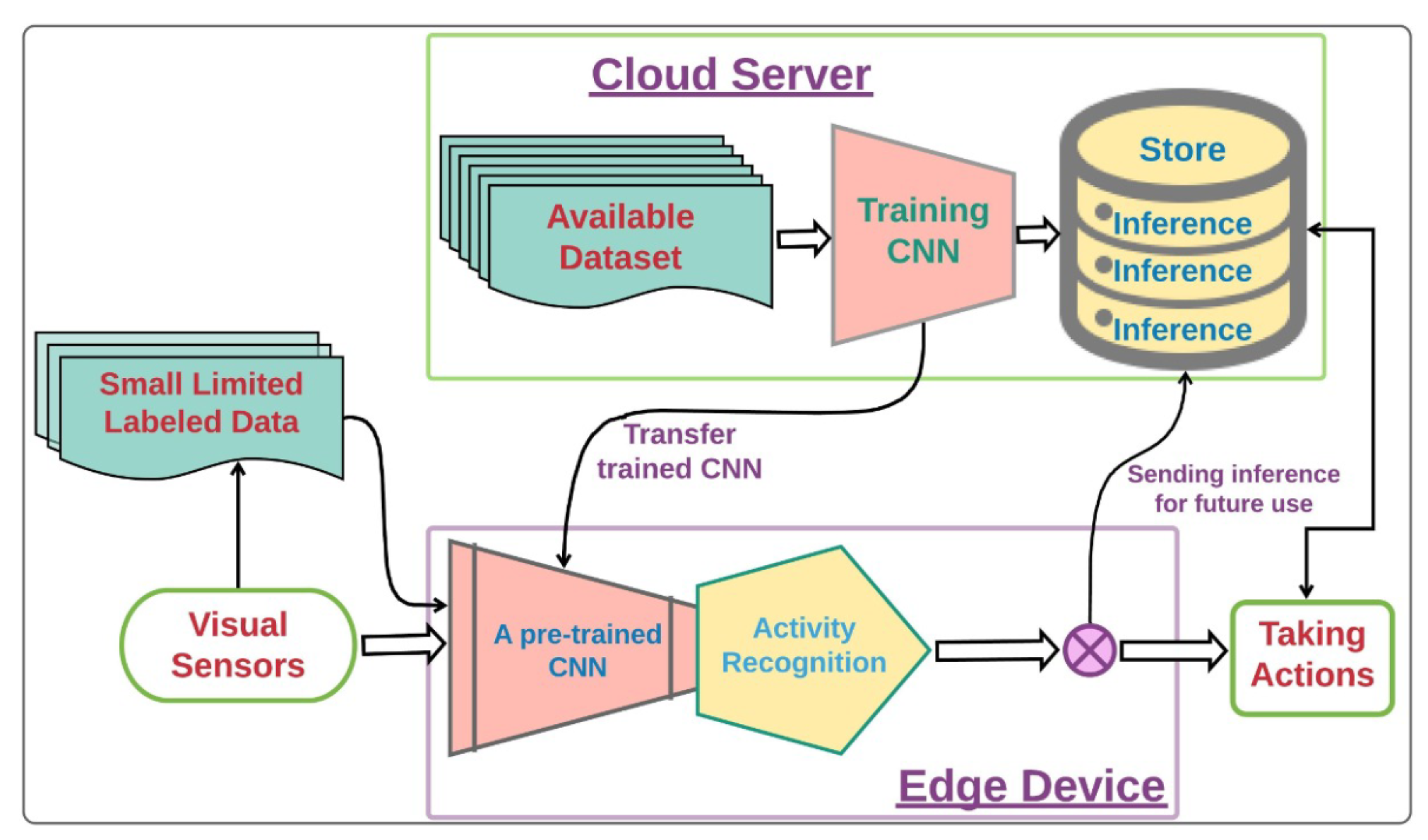
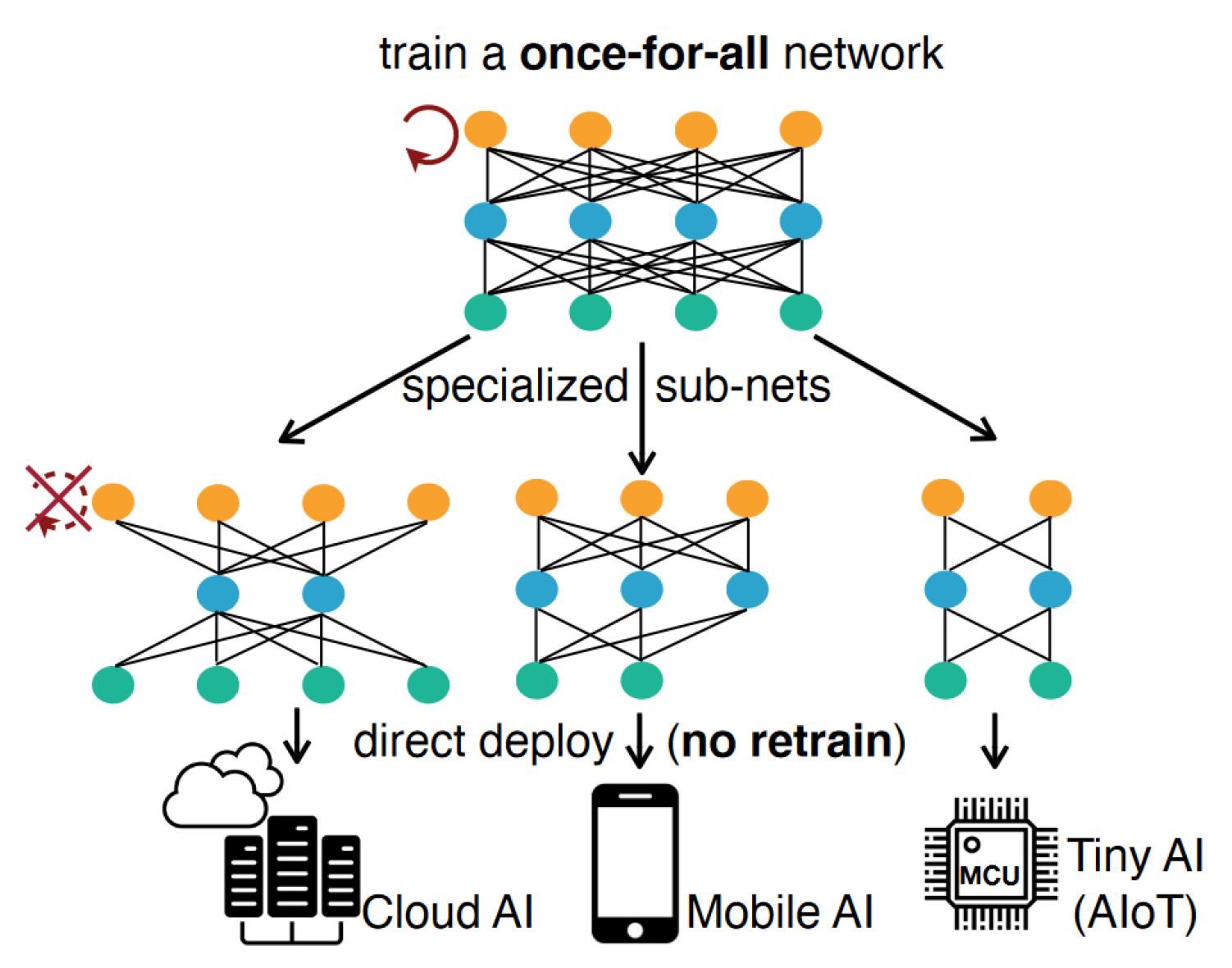
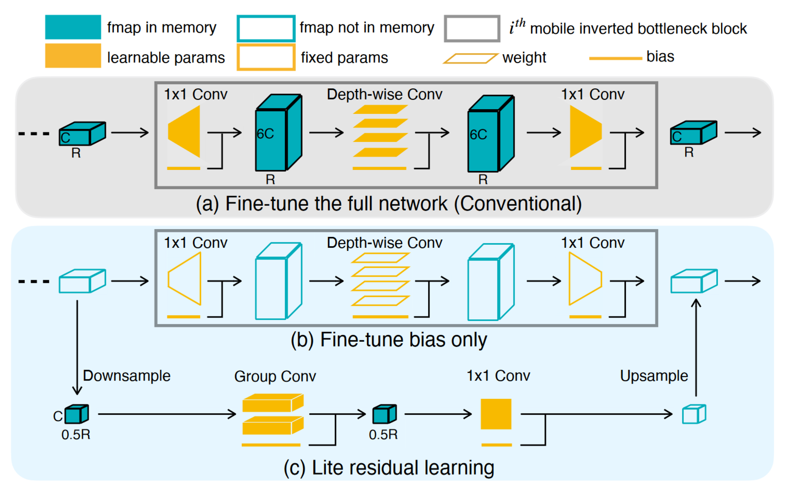
4. Transfer Learning

The first method described in the literature for IoT usage cases was transfer learning. The goal of TL is to use a previously trained ML model, e.g., a once-for-all network, and deploy it or parts from it on more resource-constrained devices such as IoT devices. If model portions are taken, some studies research the idea of adding more layers to the already chosen model part to continue training the model partially to help the model make the predictions more precisely [13,50,51,52]. This approach is included in this review because of its potential contributions to the IECC IoT and Edge layers. Furthermore, current state-of-the-art research shows that this method is actively being used in IoT use cases.

In Figure 12, an example of a once-for-all network is shown. At the top level, there is a model that is trained for a specific problem. The training may be done at a cloud data center or elsewhere with large computing resources. Subnets of the trained network are able to predict certain features for diverse problems. Thus, it is possible to select these subnets and deploy them on different architectural levels, e.g., on other cloud data centers, or mobile or IoT devices without retraining the networks [53].

Overall, the main research direction of TL is low-powered devices, as, because of their resource constraints, such devices are not able to train or run inference on large models. A survey of the literature shows that the most popular tool for implementing transfer learning is TinyML from MIT. This tool allows the utilization of low-powered devices for ML operations [50,51,52,54].

H. Cai et al. [52] created a TinyTL (tiny-transfer-learning) method using the TinyML project for continuing the training of a previously trained model more effectively on low-powered devices.

The method contains a novel approach to model training (see Figure 13). Usually, all model weights are updated, as shown in Figure 13a. However, this requires large RAM resources. The proposed solution is to leave the model weights unchanged and change only the model bias (b). However, when fine-tuning the model bias, the resulting model has low performance. For this reason, lite residual training was added (c). This allows the intermediate feature maps to be refined with a low memory footprint by adding residual mapping to the fixed gradients. With only bias updates, the layer is defined as:

$$a_i+1=F_w\left(a_i\right)+b$$

(1)

where $F_w\left(a_i\right)$ is the frozen weight i and b is the bias. However, the definition with added lite residual training changes to:

$$a_i+1=F_w\left(a_i\right)+b+F_{w_r}(a_i^{\prime }=reduce\left(a_i\right))$$

(2)

where the reduced activations ($a_i^{\prime }=reduce\left(a_i\right)$) are used rather than the full activations ($a_i$), thereby, reducing the memory footprint [52].

J. Lin et al. [51] also created an approach that allowed model training to be continued on low-powered devices with only 256 KB of RAM that was deployed on STM32F756 devices.

Figure 14 shows the ML model optimization results for low-powered devices with only 256 KB of RAM in comparison to popular ML libraries—TensorFlow, PyTorch, and others. The authors were able to achieve an approximately 2300x RAM usage decrease in comparison to PyTorch using five optimization methods:

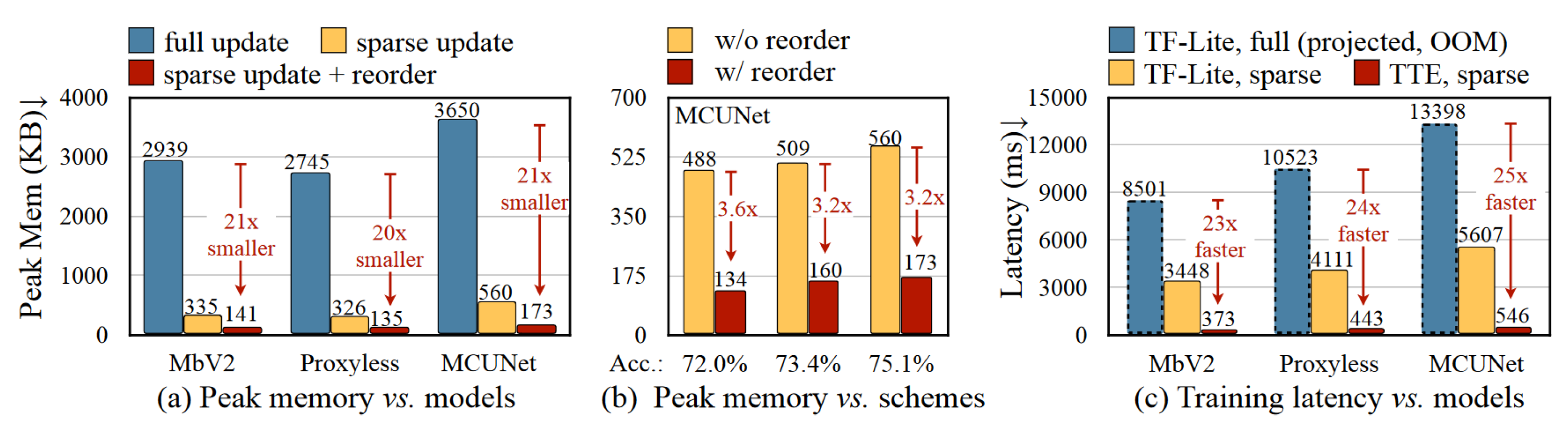
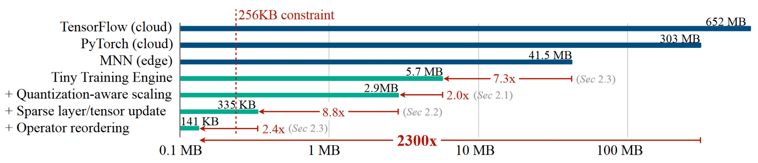
• Tiny Training Engine—The authors found the optimal training method, which includes reducing the runtime overhead, by moving parts of the computational tasks to compilation time;
• Quantization-aware-scaling—Gradients were automatically scaled with different levels of precision;
• Operator reordering—Model gradients were reordered in order to be able to apply gradient updates directly without needing to complete, e.g., the whole backpropagation cycle;
• Pruning—Model size was reduced by removing less important weights from the model;
• Sparse update—During the model training process, only the key layers were updated to reduce the new gradient impact on the whole computational load.

Figure 15 shows the results of the peak memory and latency analysis. In (a), the sparse update with reordering reduces the peak memory usage at least 20 times. However, in (b), the reordering impact on the results in three accuracy settings is shown. Reordering achieves an at-least 3.2x decrease in peak memory usage in all three cases. Lastly, in (c), the latency results are shown for the proposed solution (TTE, sparse) and TensorFlow-Lite (TF-Lite) implementations. The proposed solution outperforms TF-Lite by at least 23 times in all model settings [51].

The TinyML framework is open-source. In addition to STM devices, there are studies in which it is used in combination with Arduino Nano 33 BLE Sense devices [50,55].

Transfer learning is also used for less-resource-constrained devices such as commodity hardware that could be used as edge devices.

In cases when the initial model training requires large computing resources, e.g., to complete the training in a reasonable time period, cloud infrastructure and HPC could be used to train the model. Abu Sufian et al. [56] created a transfer-learning-based edge computing method for home health monitoring. They used cloud computing resources to train a CNN network. After training, the model was then transferred to a different location—to an edge device (see Figure 16). In this example, no optimization techniques were used. The end-user device is perfectly capable of continuing inference and training operations without the help of the cloud or HPC [56].

Transfer learning for low-powered devices is always used in combination with model preprocessing operations, e.g., pruning (removing weights in order to reduce the model size) and quantization (reducing the floating point precision relative to the precision supported by the device) in order to reach the device resource constraint limits [50,51,52]. This results in very specific implementations that are not able to adapt to ever-changing environments.

5. Method Combinations

Current state-of-the-art research analyzes the combination of distributed learning methods, including transfer learning. This is mainly because of end-user device resource constraints and the potential of one method to fix or alleviate the impact of the drawbacks of another method. For example, Chandra Thapa et al. [57] merged the SL and FL methods. The main goals were reducing the computing load that arises from running the whole model on a device in FL and the bottlenecks that arise from the sequential training manner of SL, i.e., the forgetfulness of the SL global model. The proposed method works as follows. Clients handle the client-side model portion—for example, in a medical domain, each hospital could have its own local model portion. Then, there are two servers, which are described as follows. The first is the FL server, which controls the aggregation of the client-side models into a new global client-side model. However, the forward and backpropagation functions use the client model portions and the second server—the main server—that holds the server-side model portion. This server receives all smashed data and gradients and completes the propagation server-side tasks. During backpropagation, it sends the gradients of the smashed data to the clients. However, after that, it updates the server model using the FedAvg method using the gradients it computes. Lastly, clients compute their gradients [57].

Another method was developed that changes how server-side aggregation works. Previously, aggregation was carried out on all results, denoted by SFLV1. However, with the new method (SFLV2), aggregation was carried out sequentially on receiving each client result. This results in the following communication load order when increasing the client count—SFLV2 < SFLV1 < SL. This means that the communication load for the SL+FL method using sequential aggregation of each client result achieved better results than SL and the SL+FL method that aggregates all results at once. These findings showed that a large client count decreases SL effectiveness [57].

The created methods were compared to FL and SL using the ResNet18 model with uniform data from the HAM10000 dataset. The models were split from the third layer (out of 18), where the first three layers were the client-side portion and the others, the server-side portion. For a skin pigment lesions detection task, all methods reached similar precision—approximately 76%. However, the results showed that FL and the created methods converge slower than SL—from around 20 epochs. Other tests showed that if SL is unable to converge, then SFLV1 and SFLV2 will also not be able to converge [57].

Kavya Kopparapu et al. [50] combined TL and FL in order to use FL on microcontrollers. The task of TL was to transform a CNN (Convolutional Neural Network) into a feature extractor. The authors took the last fully connected dense layer, from which a feature vector was extracted. The chosen model was not trained for a specific problem but rather for significant feature generation using large datasets—ImageNet and Visual Wake Words. Outputs of the feature extractor were used as inputs to a fully connected layer whose outputs were processed with a softmax function (adding probabilities to classes). During the training process, only the newly created fully connected layer was updated. An Arduino Nano 33 BLE Sens was chosen as the client device but a Macbook was used as the global server. Model inference and training were developed in C++ due to the absence of available libraries, although MobileNetV2 implementation from TF Lite and TinyML was used [50].

The results of the TLFL method proof of concept simulation can be seen in Figure 17. The approach without FL is denoted by a single device. Results are stable overall and all device configurations achieved similar accuracy. However, we can see that the larger number of devices achieved worse results overall than one- and three-device configurations. This may be the result of data heterogeneity, where certain features were lost during the training process. The authors mentioned that the simulation was created in order to skip having to wait for training and transfer of the weights to occur, but the results should still be identical to those of real-world deployment [50].

6. Attack Vectors

Possible attack vectors were briefly described in previous sections but these mostly concentrated on some of the possible drawbacks of the discussed method’s innate properties—the whole model gradient exchange for FL and cut layer position influence on attack performance for SL. In this section, attack vectors will be analyzed more widely from the data privacy, data security, and network security perspectives.

6.1. Attacks on Federated Learning

In FL, we essentially have three main attack vectors: trying to poison the global model by hijacking the client device and uploading infectious local model results; if a centralized format is chosen, hijacking the aggregation entity and trying to apply attacks on received ML models or also poisoning the global model; and a man-in-the-middle attack, in which the adversary eavesdrops or also poisons the model results sent to a central entity or another network node. In summary, there are two main goals—local input data retrieval and influencing the global or local model training results.

Akarsh K. Nair, et al. developed a comprehensive analysis of the state-of-the-art attacks on FL models. They define the attack types as insider and outsider attacks. Outsider attacks are from the viewpoint of an adversary who monitors the FL network communication. However, the more harmful attacks are those that are executed from the inside—insider attacks. In this case, we have malicious entities that hijack clients or central aggregators. Further attacks may be divided into two scenarios: honest but curious and malicious. A client device that listens to the network communication may be classified as honest but curious, while a malicious client device would be a client that poisons the local model. Attacks on FL models are possible at two stages—training and inference. During the training phase, poisoning and inference attacks could be carried out, because in this stage, it is possible to influence the global model and retrieve local input data. However, at the inference phase, attacks concentrate more on influencing predictions or acquiring information about model attributes. The next two main attack methods are poisoning attacks and inference attacks. Poisoning attacks can be divided into two types—model and data poisoning. The first type poisons the model directly, while the second poisons the training dataset. Conversely, inference attacks can be divided according to initial input data reconstruction and membership, property, and attribute attacks. In the first type, the goal is to retrieve the initial input data using the given global or local model, while in the latter three types, inference attacks are used to gain information about whether a specific record is part of the initial dataset (membership), what kind of properties the dataset possesses (property), and information about attributes of a specific record (attribute) [58].

Attacks on FL models are being widely researched. There are many review articles that provide a broad analysis of the current state of the art. However, most of these concentrate on the mentioned types of attacks—poisoning and inference attacks—and go deeper into their specific subtypes. For example, Chulin Xie et al. developed a new model poisoning method that uses a distributed backdoor attack rather than the conventional centralized configuration. The idea was to create a backdoor into the global model for each local model for the adversary to exploit while making sure that the global model works as usual for the intended goal of other users [59]. Virat Shejwalkar et al. evaluated poisoning attack performance on FL models. They concentrated on untargeted attacks with the goal of reducing model performance for arbitrary inputs. This was done because according to the authors, this type is more relevant to real-world examples. Their results showed that poisoning attacks are not as effective as was presumed. Even with low-cost defenses, FL models kept their robustness throughout the experiments [60]. Junchuan Liang et al. surveyed the current state of the art for poisoning attacks and defenses. Here, the authors researched targeted and untargeted poisoning attacks. They defined specific risk levels for each attack method. Among the targeted types, backdoor attacks and label reversal attacks were assigned high-risk levels. In the latter attack, the goal is to control the clients in order to make sample predictions with predefined labels. Meanwhile, the partial corruption attack type was assigned a low-risk level. The purpose of this attack is to corrupt the task of the model. Among the untargeted attack types, disruption untargeted poisoning attacks were assigned a high-risk level, while the utilization untargeted poisoning attack was assigned a low-risk level. The goal of the first attack is to make the model unable to converge. The goal of the second attack is to use the global model for secret communication [61]. Milad Nasr et al. designed white-box inference attacks for deep learning models and more specifically for FL use cases. By using gradient ascent with a malicious aggregator node, they were able to reach 87.3% inference accuracy for the CIFAR100 dataset using a DenseNet model architecture, while, using a fully connected model architecture, they reached 82.5% inference accuracy [62]. Minghong Fang et al. developed local model poisoning attacks for byzantine-robust federated learning methods. “Byzantine-robust” means that these FL methods are robust against byzantine attacks from client devices. The byzantine attack is used to massively impact the global model and its resulting accuracy by not complying with network protocols and sending random messages to the server. Byzantine-robust FL methods are able to differentiate between normal clients and these malicious clients, ignoring their updated information. However, the authors results showed using their local model poisoning attack that byzantine-robust FL methods are still vulnerable [63].

6.2. Attacks on Split Learning

Every attack mentioned in the previous section could also apply to SL methods, but only to a certain degree. For each of the possible SL configurations (see Figure 10), we could have a different attack setup. For example, if we have four nodes that train one model, the adversary could hijack one or many of these nodes and start executing poisoning or inference attacks. In comparison to FL, there are more directions the adversary could take in order to attack the model because of the many ways the model could be configured. However, it seems that the attacker should seek to control more nodes than in the federated learning setting because the results of the attack probably will not be as good when the adversary controls only one client node with, e.g., 3 out of 15 layers, compared to when an adversary controls a node with the whole model in FL. Nevertheless, poisoning of the model is still possible; however, the success of inference attacks is more limited due to the distribution of the model to more nodes. This increases the complexity required to implement the attack because the adversary needs to hijack more network nodes to increase the chances for the attack to be successful.

Attacks on SL models are also a popular research direction, but sadly no comprehensive article was found that covered the whole scope of attacks in SL, as it was done in [58] for the FL method. However, many articles were found that considered the problem from the point of view of the attack scope, e.g., inference attacks. For example, Maria Rigaki et al. created a survey of privacy attacks in machine learning. Here, the authors delved into DL, including SL. They emphasize that the central node in SL model training is still highly impactful because it receives all intermediate results and may execute attacks on these results or on all the participating nodes. They mention that data reconstruction attacks in SL are still possible. For example, when there are two portion configurations with clients and the central server, the server could reconstruct the initial data by using the received client portions of the model [64]. Mingyuan Fan et al. researched the robustness of split learning when the adversary has hijacked the server and has access to intermediate layers of the model. The configuration corresponds to Figure 10c. In this case, the attacker has no knowledge of the labels as well as input and output data. In order to compensate for the missing input layers, the authors propose a shadow model training approach. The goal of the attacker is to direct the model to the wrong predictions for given samples. The results show that for some cases, it is possible to achieve an approximately 45% reduction in accuracy, averaging 31.92%, 27.37%, 38.45%, and 39.04% for the ResNet, EfficientNet, DenseNet, and MobileNet model architectures, respectively, [65]. Behrad Tajalli et al. developed a new backdoor attack on split learning models and analyzed its performance. This attack was tested on the vanilla SL configuration (see Figure 10a). In the threat model, the adversary controls only the server node. Two cases were implemented. In the first case, the server utilizes a surrogate client node that other clients do not know about to inject the backdoor trigger. In the second, an autoencoder was used to inject the backdoor trigger that processes the normal client smashed data into poisoned smashed data. The results showed that SL is robust against such attacks. The authors emphasize the difficulty of injecting backdoor triggers with only the server-side portion of the model [66]. Dario Pasquini et al. proposed a new attack model—the feature-space hijacking attack. Here, they also used the SL label protection configuration (Figure 10c). The adversary controls the server but has no information on client models and the task of the whole model. However, the adversary has a dataset $X_{pub}$ that contains data from the same scope as the client input data. For example, if client data contains images of cars, then the adversary dataset will also contain such images. The goal here is to replace the existing task of the model and shift the clients towards a specific feature space chosen by the malicious server. In such a case, the server will be able to recover the private local input data by inverting the known feature space. This attack is a specialized type of inference attack and reached below 0.05 reconstruction error for image datasets—MNIST, Fashion-MNIST, CelebA, and Omniglot—being able to determine from which client data the reconstructed data came. However, the success of this attack is related to how close the dataset $X_{pub}$ is to the scope of the client dataset [67]. Oscar Li et al. analyzed label leakage in vanilla SL (see Figure 10a) exploiting a private intersection protocol, in which the client (non-label party) finds intersections with server-side data (label-party). With this approach, a malicious client may retrieve label information. Their results showed that it is possible for the malicious client to retrieve label information with up to a 100% success rate without using any mitigation methods [68].

6.3. Attacks on Transfer Learning

The general idea of attacking TL models is the same as that in the previous sections. Imagine we have a model that is trained on a cloud data center because of the “unlimited” resources it provides for us to train a large model with a massive input dataset in a reasonable time. The cloud virtual machine (VM), on which the training is done, could be hijacked, resulting in potential leakage of the input data or the adversary poisoning the model. If the training has already been done and the VM has no direct access to the initial input data, the model could be used for inference attacks. From the communication perspective, the man-in-the-middle attack could also be executed to poison the model on its way to the end-user or retrieve it for later inference attack execution. By hijacking the end-user device, the same attack vectors could be exploited, and possibly more vulnerabilities could be used to gain information or access to the entity that trained the model.

Attacks on TL are not a very popular research direction, although some articles can still be found. For example, Bolun Wang et al. developed a method for poisoning the input data for inference in order to make the model misclassify the inputs. In the threat model, an adversary has knowledge about the transferred model (teacher) but not the actual end-user device model (student), and the end user can add some changes to the model. By analyzing the layers of the teacher model, the authors developed a perturbation technique to perturb samples so that they would be classified as images from other classes. The resulting perturbation goal was to still look similar to the original sample but to be misclassified. With a reasonable perturbation level, the authors achieved approximately 90% effectiveness with this attack for the face recognition task [69]. Yinghua Zhang et al. analyzed the robustness of a fine-tuned transferred model against fast gradient signed method (FGSM) attacks when the target is accessible to the adversary (white-box attack). This attack also has the goal of making the model misclassify a given input without changing the general characteristics of the image in order for humans to be unable to distinguish between the poisoned and real image. The results showed that a fine-tuned model is robust against such attacks. However, the authors proposed an attack for a black-box approach, where the adversary has access to the source model of the fine-tuned model. They reached the same 90% accuracy with approximately the same perturbation level as in the previous article on some datasets [70]. Xue Jiang et al. developed a poisoning attack in order to create backdoors in TL models for brain–computer interfaces. The idea is to select random samples from the initial dataset and add crafted triggers to these samples to change their classes to the chosen class. When this poisoned data is used in TL training, the backdoor is successfully set. As a result, it reached an average of around 90% attack success rate using various model architectures and datasets [71]. Another backdoor attack model was proposed by Shuo Wang et al., in which the goal was to defeat defenses such as pruning, retraining, and input preprocessing. They used ranking-based sample selection mechanisms to overcome pruning and retraining defenses. In addition, the authors created an autoencoder for robust trigger generation to defeat input preprocessing defense, as well as defense-aware retraining—retraining the model with a poisoned dataset after pruning. As a result, they reached over 90% attack success rate on image and electrocardiography recording (ECG) datasets [72]. Yang Zou et al. evaluated membership inference attacks against TL models. They emphasize three potential directions: the attacker has access to the teacher model, with the goal of inferring a sample from the teacher dataset; the attacker has access to the student model, with the goal of inferring a sample from the teacher dataset; and with the same access privileges, the attacker hopes to infer a sample from the student dataset. They reached 75.3% accuracy for the first direction, approximately 49% on average for the second, and approximately 89.4% on average for the third direction. However, these results were for models with the same architectures. After that, experiments were carried out in which student and teacher models were different. Here, they achieved an Area Under the ROC Curve (AUC) of 0.9. A higher AUC value means better attack performance. In conclusion, an unknown model architecture was not an obstacle to the membership inference attack in TL [73].

7. Attack Mitigation

To summarize, the main attack methods used are model poisoning and information inference attacks. Other attacks such as for IoT devices, edge devices, or cloud VM hijacking using vulnerabilities of hardware, software, firmware, or network configuration are out of scope for this article. Given the main attack methods, we need a method for limiting access to the initial model as well as limiting the information that the model learns. Firstly, by limiting access, we would secure the model from an adversary acquiring the model in plaintext, meaning we could implement secure communication channels; we could also secure access to the model itself, for example, by encrypting it. Secondly, as, even when we use encryption methods that require decrypting the model for aggregation or applying it to client devices in FL, the model can still be retrieved by an adversary, we need to implement a more robust approach, for example, using data perturbation techniques. In this case, even though the adversary still may launch the mentioned attacks in these scenarios, with perturbation methods, we could limit how much the model remembers–although this requires a trade-off between model utility and data privacy. Nevertheless, with this approach, we could have more confidence about data not leaving the data owners (e.g., IoT or edge) device because of the added noise from using perturbation methods.

7.1. Secure Aggregation

Aggregating data that were received from multiple parties, where no party reveals its data to others (even the aggregator), is called Secure Aggregation (SA). With this method, the client can be certain that the server will only receive the aggregated result and not the individual client data [74]. As a result, we achieve better security by obfuscating the model until the aggregation is finished, as well as improving the privacy of the client data to the extent of the resulting global model. This is because, even if an adversary has retrieved information from the global model, e.g., specific records, he has no direct information about which client this information came from. In FL, an adversary that is located on the aggregator device could retrieve only the global model, while an adversary located on the client device could possibly control the local model that is sent to the aggregator and retrieve the global model. In this case, an important problem may arise: a malicious client may poison the local model in order to influence the global model. The aggregator would not be able to assess the legitimacy of the received local model because it has access only to the aggregated result. For this reason, SA is for limiting aggregator and network adversary access to client locally trained models. With this in mind, at the very least, an adversary would have to hijack each client device in order to retrieve each client’s local model.

7.1.1. Secure Multi-Party Computation

One of the methods by which SA is being implemented is secure multi-party computation (SMPC, sometimes also known as MPC or SMC). With this, we can perform computations on data from many parties without disclosing any party’s private inputs to other parties. Parties agree upon what function to compute and then use an SMPC protocol to jointly compute the output of the chosen function on their secret inputs without revealing them [75]. However, SMPC secures only the process and not the output of the function. That is why the output may still leak information. In addition, inputs are also not secured. An adversary may input false information and still be able to jointly compute the function [76]. The key part of this method is that there is no third party that computes the function. Only the data owners can do this computation [75]. There are two main basic primitives:

• Secret sharing—In a (t, n)-secret sharing scheme, we split the secret s into n shares, where any t − 1 shares reveal no information about s, while any t shares allow the reconstruction of the secret s. In this scheme, t could also be equal to n, resulting in (n, n)-secret sharing schemes, where all n shares would be required to reconstruct the secret [75];
• Random oracle—This is a heuristic model for security of hash functions, treating them as public, idealized random functions. In this model, all parties have access to the public function H: ${\left\{0,1\right\}}^{*}$→${\left\{0,1\right\}}^k$, implemented as a stateful oracle. On input x $ϵ$${\left\{0,1\right\}}^{*}$, H looks up its history calls. If H(x) had never been called, H chooses a random $r_x$$ϵ$${\left\{0,1\right\}}^k$, remembers the pair x, $r_x$, and returns $r_x$. If H(x) had been called before, H returns $r_x$. As a result, this method is a randomly-chosen function ${\left\{0,1\right\}}^{*}$→${\left\{0,1\right\}}^k$ [75].

SMPC is a quite popular method for securing joint computations in FL, although frequently it is implemented further from its definition, e.g., using a third party for computing a function. For example, Keith Bonawitz et al. created a SA method using secret sharing. The authors used SMPC for computing sums over vectors securely using a third party with limited trust for the FL scenario. In addition, they proved that this method is also secure in the random oracle model [74]. David Byrd et al. also used secret sharing to create secure FL. The authors based their SA protocol on the implementation from Bonawitz et al. [74]. However, they also used differential privacy to improve initial data owners’ privacy [77]. There are many more similar SMPC implementations such as [78,79,80].

7.1.2. Homomorphic Encryption

When computations are held at a third party that is not trusted, e.g., an aggregator entity (the server) in FL, clients can use homomorphic encryption (HE) to encrypt their local models and send them to the server, where the server aggregates the models while they still are encrypted. For this reason, the aggregator never receives access to any local models and even the aggregated result but only computes the aggregation and sends the encrypted result back to the clients. The difference between SMPC and HE is that SMPC does not require a third party for computations, while, using HE, there is usually a third party that computes a function on homomorphically encrypted datasets [75]. Nevertheless, both HE and SMPC are sometimes used together [81]. The encryption scheme can be defined as homomorphic if

$${\forall }_{m1,m2}ϵM,E\left(m1\right)oE\left(m2\right)=E\left(m1om2\right),$$

(3)

where $E\left(m_n\right)$ is the ciphertext of message $m_n$ from a set of messages M, and o is the operation that is used with the ciphertexts, e.g., addition or multiplication [82]. This method could also be used in a decentralized setting. For example, in FL, one of the clients could be the aggregator of other client models and control the aggregation and encrypted global model distribution process. There are three HE types divided according to their operations and application frequency:

• Partially Homomorphic Encryption (PHE)—Allows the execution of one type of operation an unlimited amount of times;
• Somewhat Homomorphic Encryption (SWHE)—Allows the execution of a few operations a limited amount of times;
• Fully Homomorphic Encryption (FHE)—Allows the execution of any operation an unlimited amount of times [82].

The research for ML use cases mostly focuses on the third type—FHE. However, articles using other types of HE can also be found. For example, Haizhou Liu et al. used Paillier PHE with FL for securing the models from the central aggregator, while the server only executed the aggregation operations [40]. However, Paillier PHE by definition allows only the addition operation and a few extra operations under certain conditions. That said, there are more recent methods that improve upon the Paillier scheme [82]. In the recent literature, the main focus is on FHE and more specifically, the Cheon–Kim–Kim–Song (CKKS) scheme. This scheme fully supports FHE and even floating point numbers, which is crucial for ML use cases [83]. For example, Jing Ma et al. developed an FL model with multi-key homomorphic encryption using the CKKS scheme [84]. Overall, the CKKS scheme is widely researched, e.g., in FL [39,41,85,86], SL [87,88], and TL [86,89,90].

However, some publications [19,91] note the high computational costs that this method brings; for example, with such novel methods as homomorphic encryption. This results in them being of limited use for low-powered devices on the edge and constrains us from using such devices. As a result, more powerful computing power should be used, e.g., cloud computing solutions.

7.2. Robust Aggregation

Securing the models in DL is an important step towards a more robust deployment. Sadly, security methods can get you only so far, because they can give no implicit promises about the rigidness of the aggregation. To be more precise, an aggregator in FL or an intermediate node in SL is not obligated or even able to check received inputs and deduce whether or not the data are legitimate or should be discarded. For example, in centralized FL using HE, an adversary may control one of the clients in the network, poisoning the local model in order to influence the global model. When the aggregation takes place, there is no part in the communication protocol in which a node in the network checks the legitimacy of the received model. Thus, an adversary may train a local model far from the global characteristics and as a result, poison the global model. Similar to IoT, there is a requirement of root of trust (RoT). For example, Xiaoyu Cao et al. showed that in the current state of the art, there are no root-of-trust methods in FL [92]. This led the authors to propose an approach for establishing RoT in FL.

Figure 18 illustrates their proposed RoT method in FL. In the first step, clients and the server train a local model, whereby, clients have their own local datasets but the server has a root dataset with similar characteristics. Next, clients send their local models to the server for aggregation. The server now compares the received models to the server model and adjusts the results relative to the server model. After that, aggregation is done, and the global model is sent to the clients [92]. With this approach, we, to a certain degree, are able to verify which clients might be trying to poison the global model. More specifically for FL use cases, such methods are defined as robust aggregation schemes. The main goal is to analyze client interactions in the network and their sent models and to decide whether or not the client is malicious, as a result, attenuating or completely removing their models from further aggregation or training operations [15]. However, in order for an entity in the network to improve certainty as to which clients can be trusted, new vulnerabilities are introduced, such as the server having direct access to the local model results in FL as well as data located on the server.

Some articles discuss the use of blockchain technology to improve the robustness of the aggregation scheme. The working principle for this approach is to incorporate blockchain primitives into FL networks:

• Transactions—The data to be stored on the chain, sent from one of the nodes in the network;
• Shared ledger—An accounting mechanism of all verified transactions in the blockchain network;
• Consensus mechanism—In order to verify a transaction, a network consensus has to be reached in which network nodes agree upon whether or not to accept a transaction;
• Peer-to-peer (P2P) networking—Decentralized communication mechanism;
• On-chain and off-chain storage—Data that are kept on-chain are usually smaller in size in order for the chain not to become too large, e.g., metadata about transactions. That is why off-chain storage is used, e.g., the interplanetary file system (IPFS), for storing large data such as ML models, as is the case in FL [93,94].

By using blockchain technology, we acquire traceable information of all node results in the network using the shared ledger that holds information on all transactions (local model updates) that are accepted using the consensus mechanism, as, for example, transactions that are unaccepted may be malicious. By default, the use of blockchain technology allows the creation of an FL network in a decentralized fashion using both on-chain and off-chain storage for metadata and larger model storage, respectively. As a result, e.g., in FL with this approach, we are able to track each model update in the network in a decentralized setting. For example, Mansoor Ali et al. proposed a solution for malicious node detection in cross-silo FL using blockchain technology. The authors used blockchain technology in silos to be able to trace back model history in case the aggregated model has deviated from the expected model result [94]. A deeper dive into blockchain usage with DL is out of the scope of this article; however, survey articles, e.g., refs. [93,95] hold a great deal of information regarding this specific topic.

7.3. Differential Privacy

In addition to security and robustness against poisoning attacks, the privacy of local data owners is a hot topic in current research. The main problem is that the trained model memory holds information about the data it uses for training, meaning that the models remember certain parts of the initial data records, which results in privacy leakage, e.g., even specific record retrieval. Christopher A. Choquette-Choo et al. analyzed defenses against membership inference attacks in ML use cases. The main conclusion of their work was that the only current defenses against such attacks are differential privacy (DP) and L2 regularization, with DP providing the strongest defense overall [96]. Christopher Briggs et al. reviewed preserving privacy in FL. They found that in addition to perturbation methods such as DP, anonymity methods, e.g., k-anonymity and its successors—l-diversity and t-closeness—are a possible research direction; however, the research showed that the current state of the art has directed the research focus onto more rigorous approaches such as the aforementioned DP. This is mainly because anonymity methods are prone to leaking information under linkage attacks. Linkage attacks use existing public datasets to link anonymized datasets in order to deanonymize the private dataset, for example, to be able to identify specific individuals [19].

Differential privacy also provides defense against backdoor attacks. Sun et al. [97] researched whether or not you can defend against backdoor attacks in FL. One of the defenses they mentioned is weak differential privacy. In this approach, in comparison to vanilla DP, the added noise amount is smaller, hence the name Weak DP, but the approach still provides the defense characteristics. A similar direction has also been researched by Miao et al. [98]. Here, they used DP in combination with clip norm decay with the idea of reducing the clipping threshold in order to increase the accuracy as well as defending against backdoor attacks [98].

DP was first defined in 2006, where the main purpose was database obfuscation in order to replace anonymity methods. The main goal of DP is to perturb the data in order to obfuscate individual records from being identified while keeping the general characteristics of the dataset intact [99]. DP has many implementation approaches, but they are mostly related to two baselines:

• ($\epsilon$)-DP—The original DP method with the most robust privacy rules. This method is defined as follows:

  $$Pr\left(M\left(x\right)ϵS\right)<=e^{\epsilon }Pr\left(M\left(x^{\prime }\right)ϵS\right)$$

  (4)
  The probability of acquiring a result, part of S, where $S\subseteq Range\left(M\right)$, when using a mechanism M on a given dataset x is less than or equal to $e^{\epsilon }$ or approximately $1+\epsilon$, multiplied by the probability of acquiring a result, that is part of the same S, applying the same mechanism M on an adjacent dataset x’, where the difference between datasets x and x’ is at most one record. Here, there is only one parameter to tune—$\epsilon$—where, the smaller the $\epsilon$, the more private the end result, because the difference between adjacent datasets will be smaller. Best practices describe choosing the $\epsilon <1$. However, this method adds too much noise to the result, which is why this method is not used in ML use cases, because of the high perturbation level resulting in too high utility loss [100,101];
• ($\epsilon ,\delta$)-DP—To make DP more friendly to ML use cases, a relaxation of ($\epsilon$)-DP was proposed, by adding an extra parameter $\delta$, such that the definition changes to

  $$Pr\left(M\left(x\right)ϵS\right)<=e^{\epsilon }Pr\left(M\left(x^{\prime }\right)ϵS\right)+\delta$$

  (5)
  In this format, the new parameter adds the possibility of incorporating less noise during the application of the mechanism, resulting in better utility. It follows that an adversary can successfully identify $\delta \ast n$ records. For this reason, the recommendation for the new parameter is to set $\delta <<\frac{1}{n}$, where n is the dataset size. In addition, the definition holds for $\epsilon <10$. However, usually in practice, smaller $\epsilon$ values are chosen such as below eight or even smaller [100,101].

There are many mechanisms M used that add noise to the adjacent datasets in order to implement DP in both of these approaches. For example, in ($\epsilon$)-DP, the Laplace mechanism is the baseline mechanism. Here, added noise is taken from the Laplace probability distribution function (PDF). This mechanism limits its usage to only scalar data. However, in ($\epsilon ,\delta$)-DP, the baseline is the Gaussian mechanism, which does not promise ($\epsilon$)-DP privacy guarantees. Here, the noise sampled from the Gaussian PDF results in less added noise in comparison to the Laplacian because, even far from the center of the PDF, the noise is much greater in the Laplacian PDF than it is in the Gaussian PDF. In addition, the $\delta$ parameter is employed to add extra noise relaxation. This mechanism is used in popular DP ML approaches, e.g., DP-SGD, which is a differentially private optimizer. Similar to the Laplacian, the Gaussian mechanism is also limited to scalar values. There are many more DP mechanisms, for example the Exponential mechanism, that can work with more arbitrary data types, such as text [101].

DP can be applied in many scenarios, whether it is with a central entity that executes the DP method or in a distributed manner, e.g., similar to FL, where each node adds DP noise to its local model result. These two types are defined as

• Global differential privacy (GDP)—In this approach, there is one node that applies DP to the data, e.g., the global model in FL, and other nodes just send and request data from this node. For example, in FL GDP, clients would send their models without adding DP locally, and the aggregator server would add DP to the aggregated model and send the global model back to the clients [101];
• Local differential privacy (LDP)—Not adding the DP noise locally creates potential privacy leakage because the data can be intercepted on its way to the node that applies DP. That is why LDP was proposed in order for the data owners to apply DP locally; however, this results in higher utility costs because the composite noise level increases in comparison to GDP [13,101,102]. Even without DP, the FL method may not converge in the training process if the data distribution varies largely from clients [13]. Thus, by adding DP, and especially LDP, the resulting convergence rate could decrease substantially. However, some articles research the idea of shuffling the sent data before handing it over to the aggregator. This results in a higher privacy level with a less or equal amount of noise [103]. Nevertheless, LDP is popular among FL implementations, and many articles can be found that use the LDP method in addition to FL [29,104,105,106,107,108,109]. For example, Arachchige et al. proposed a framework that uses FL, DP, blockchain, and smart contracts for ML in Industrial IoT. Here, the DP was used to obfuscate the model in a local data-owner device before encrypting it. After that, it was placed in an off-chain storage medium [106]. Meanwhile, Lichao Sun et al. proposed a new LDP method optimization technique in order to fight the DP noise explosion, arising from model weight high dimensionality, as well as to fight different model weight ranges in different layers [109].

DP usage is also being researched in SL use cases [43,57,110,111,112,113,114]. For example, Xin Yang et al. proposed a transcript private split learning for label protection using split learning. The authors focused on protecting the label information by adding DP noise to both the gradients and the model updates [112]. Hang Xu et al. developed two denoising techniques for using DP with SL. In addition, the authors mention that the denoised result has better security against state-of-the-art attacks in comparison to baseline DP protection methods [113].

In TL, the usage of differential privacy is also being researched [115,116,117,118,119]. Isaac Shiri et al. proposed a new method for preserving privacy for positron emission tomography (PET) image artifact detection using FL and TL. They used the previously proposed sequential FL method that uses the TL method to exchange models in a sequential manner [120], to which the authors added DP in order to increase the privacy of PET image owners [117]. Yizhe Li et al. proposed a new teacher–student model private training approach, that they compared to transfer learning. The authors showed that their approach with DP achieves better utility with higher privacy in comparison to TL with DP [118].

In order to apply DP in distributed learning methods using LDP, certain properties need to be taken into account. Firstly, there is the sequential composition that states that if DP is applied sequentially on the private data, then the resulting privacy level will be equal to the sum of all $\epsilon$ values. Next, in parallel composition, when applying DP on a disjoint dataset, the resulting privacy level will be the maximum $\epsilon$ value. Lastly, a post-processing property is at play. Here the composition of a private mechanism $M_1$ and a non-private mechanism $M_2$ still results in a privacy level identical to the mechanism $M_1$ [103,121].

The application of DP in the ML scope in general could take place at four stages: at the input level, during training, on the resulting model, or on the predictions. The main idea is that the closer you are to the end result (the predictions), the better the privacy vs. utility trade-off will be. The most popular DP application stage is during training using a chosen DP optimizer, e.g., DP-SGD [101]. To implement DP into your solution, for a simple ML model without using DL methods, one could incorporate DP by analyzing the privacy–utility costs using accountant mechanisms [101]. Such mechanisms are included in popular ML libraries, e.g., TensorFlow and PyTorch [122,123,124]. These mechanisms take into account the hyperparameters of DP methods and data size and output the privacy level that will be achieved if the DP is applied using these parameters to the chosen dataset [101]. However, current research shows that calculating a posteriori the achieved privacy level is still important in order to audit the DP application process because hyperparameter tuning is complex and may result in unwanted and unnoticed errors. That is why there are methods to calculate approximate lower and higher limits of the proposed privacy level [101,125,126,127,128]. For example, Florian Tramèr et al. debugged a recently proposed DP training mechanism, proving with ∼99.9% confidence that the proposed method reaches not the proposed $\epsilon =0.21$ lower bound privacy level but rather $\epsilon >2.79$. This was done by using strong membership inference attacks [127]. Zanella-Béguelin et al. proposed a Bayesian estimation method for DP privacy level bound detection. As a result, they exceptionally reduced the necessary computing resources as well as achieved from 34% to 40% privacy level interval reduction in comparison to previous methods [128].

In addition to auditing, DP privacy–utility a priori analysis is being researched. The main reason for this is the great effort that is required in order to find optimal privacy and utility values. With this, the goal is to decrease the necessary time and computing resources in order to find the target privacy–utility trade-off using empirical risk minimization (ERM). However, such research is limited to specific use cases, e.g., objective function perturbation [125,129]. For this reason, implementers could use more abstract guidelines. For example, Ponomareva et al. from Google created a comprehensive guide on how to apply differential privacy in ML use cases [101].

8. Tools

In order to create DL implementations into IECC use cases, one could use existing tools for each method. However, doing everything by hand is still an option. For example, implementing FL using only base ML libraries such as Tensorflow or PyTorch. Federated learning has risen in popularity quite considerably, which is why many tools are available. Not only implementation tools but also benchmarking and simulation tools are being created and researched in order to analyze the performance of various FL settings. Currently, some research is focused on comparing the existing tools. For example, Guendouzi et al. compared current FL tools, concentrating on their node data partition configurations and scalability, also mentioning the diverse flexibility, privacy, and security features. Some tools are more of a configuration type without great adaptation possibilities, but others allow almost limitless adaptation because the tool is open-source and programmable rather than configurable [130,131]. Rodríguez-Barroso et al. created a software tool analysis concentrating on FL with DP. In addition, the authors proposed their own framework sherpa.ai. The authors analyzed each FL framework in detail with respect to their privacy features, FL aggregation mechanisms, documentation quality, support of ML libraries, and other characteristics [131]. Articles in which a new FL framework is proposed also usually have some analysis of other alternative tools [132,133,134]. For example, Beutel et al. presented the Flower open-source FL framework. Comparing heterogeneous client support (clients with different hardware), ML framework agnosticism (different ML library support), communication agnosticism (different communication protocol support), language agnosticism (different programming language support), and many other features with other frameworks [133,135].

The split learning method is not as popular as FL. For this reason, tool availability can be a problem. However, Chaoyang He et al. developed an FL framework FedML that supports split learning as well. In addition to other features, the authors compared the support for SL with other frameworks. Two tools were found that also support SL: PaddleFL [136] and PySyft [137]. With all three of the SL supporting tools being open-source, the proposed FedML tool was described as better than the alternatives in relation to FL, benchmarking, flexibility, and computing paradigm features [134]. In addition to this, more articles can be found that propose frameworks that include or concentrate on SL. Unfortunately, they do not provide public access to these tools [138,139]. Nevertheless, as with FL, manually creating split learning implementation is a possible direction. For example, for using SL together with FL, one could add SL functionality to an open-source FL tool similar to FedML, PaddleFL, or PySyft.

In transfer learning, the tools could take a wide range of directions. For example, some tools focus on ML model exchange in teams [140], some on heterogeneous edge and IoT hardware and optimization [141], and others on optimization for specific hardware vendors such as STMicroelectronics [142]. However, all these tools are part of MLOps platforms—cloud-based machine learning operations because the knowledge transfer is used in addition to model training and optimization in the cloud. Hymel et al. proposed the edge impulse framework. The authors compared the tool with seven more alternatives from large companies such as Amazon and Microsoft in relation to five features—data analysis and collection, digital signal processing (DSP) and model design, embedded deployment, autoML (assisting non-domain experts in developing ML models), active learning (maximizing model utility using as few samples as possible [143]), and IoT monitoring and management. The proposed tool was shown to support every feature fully except the last one (IoT monitoring and management), which it supports only partially. However, it shows the best result overall [141].

In the scope of the IECC, the implementer should probably focus on tools that concentrate on or at least include features concerning edge and IoT deployments. In FL, the Flower framework is one such example. As their focus is on client heterogeneity, clients can have various hardware architectures, base ML libraries, and programming languages. In SL, the choice is more difficult because there are not many alternatives. However, FedML has support for edge and IoT devices. For this reason, this tool could also be adopted for FL and SL implementations. For TL, overall, the most flexible tool for the IECC seems to be edge impulse because it focuses on both the training on the cloud and optimization for different hardware architectures including edge and IoT devices; thus, having the flexibility of choosing the end-user device. Nevertheless, the possible alternatives that were looked into while analyzing the edge impulse framework [141], e.g., the Azure ML & IoT tool [144,145], which also showed good results, and others [140,142], should be taken into account.

9. Discussion and Future Directions

Technological advances have brought us to a time where even small IoT devices are able to be part of MLOps tasks. This helps to establish IECC layer—IoT, edge, and cloud—integration into one seamless continuum by distributing the computational burden throughout the whole continuum. However, the further we travel from the cloud, the less computing power will be available. Thus, for large model training, with high floating-point precision, the utilization of power-constrained devices will not be an option.

Distributed learning holds various research directions for implementing ML in the IECC. Federated learning helps to move further from centralized data servers by distributing the models to all data owners and training the model there. Split learning tries to fix the whole model training problem by splitting the model into parts and distributing it to many devices in order to reduce the computational complexity by using many devices. In addition to DL, transfer learning allows the use of the teacher–student training model for knowledge transfer from high-computing-power nodes to more power-constrained nodes. All these methods and their combinations alleviate some of the innate implementation challenges that the IECC has in order to implement ML in the continuum. Nevertheless, as research has shown, there are certain challenges regarding the security, privacy, and robustness of the methods. For example, in FL, there is a security and robustness trade-off. In order for other nodes or the central aggregator to check the quality of the received model, it has to be able to retrieve it in plaintext, either directly or by deciphering it. Thus, if the aggregator is malicious, it can try to execute, e.g., inference attacks on the received model. We could perhaps overcome this problem by using a homomorphic-encryption-type approach, which would allow us to check the received models with an algorithm that outputs, e.g., the quality or distance from the current global model while keeping the models encrypted. From the privacy perspective, in differential privacy, there also is a trade-off between privacy and utility. Therefore, that the implementer has to choose what is the most suitable trade-off for them. Here, the implementation steps are still not entirely clear, but certain articles have defined specific guidelines about hyperparameter tuning [101]. Because of the high implementation complexity, DP auditing is being researched, showing that the privacy level can be determined with lower and higher bounds after the DP has been applied. However, there is still a lack of precise privacy level detection.

There are many available tools for DL and TL method implementation, both open-source and proprietary. Some articles have analyzed how the tools compare using various metrics, e.g., client-count increase in FL and model design support in TL [133,134,141]. Our review showed that federated learning has the most tools available, followed by TL and then SL. Split learning had no individual tools, but rather has been added as a feature to some FL tools [134]. In the IECC, all these tools could be of use, e.g., to port a model from the cloud, using TL, to edge and IoT layers. FL could be used to control federated training using edge devices as servers and IoT devices as clients or decentralized, in which SL could be used as the computation distributor to many client devices, resulting in a framework that would combine all these methods.

10. Conclusions

This article presents a review of distributed learning concentrating on the implications in the field of the IoT–Edge–Cloud Continuum. The methods of DL and transfer learning were investigated, including the tools to use for implementations. Attack vectors for all these methods were also looked into, allowing us to provide information about their mitigation using privacy, security, and method robustness-enhancing techniques. Differential privacy was found to be the most popular and effective tool for establishing privacy protection. However, because of the high implementation complexity, research has shown that a good practice would be to include auditing in order to check the privacy level after the DP application. Securing the data in DL can be established with secure aggregation using secure multi-party computation and homomorphic encryption. However, the resulting performance may be downgraded because such methods require a higher amount of computational complexity. The robustness of the implementation can be developed by creating protocols that require establishing root of trust. For example, blockchain technology was found to be a popular research direction in this area. In the end, achieving the balance between ML model privacy, utility, and robustness is a hard problem that is actively being researched. Each heterogeneous implementation of any DL approach, including TL, requires a great amount of work to configure the parameters of the chosen architecture to achieve a goal, or more frequently, a compromise between the costs of computation, security, privacy, and utility.

References

1. Moreschini, S.; Pecorelli, F.; Li, X.; Naz, S.; Hästbacka, D.; Taibi, D. Cloud Continuum: The definition. IEEE Access 2022, 10, 131876–131886. [Google Scholar] [CrossRef]
2. Bittencourt, L.; Immich, R.; Sakellariou, R.; Fonseca, N.; Madeira, E.; Curado, M.; Villas, L.; DaSilva, L.; Lee, C.; Rana, O. The internet of things, fog and cloud continuum: Integration and challenges. Internet Things 2018, 3, 134–155. [Google Scholar] [CrossRef]
3. Kampars, J.; Tropins, D.; Matisons, R. A review of application layer communication protocols for the IoT edge cloud continuum. In Proceedings of the 2021 62nd International Scientific Conference on Information Technology and Management Science of Riga Technical University (ITMS), Riga, Latvia, 14–15 October 2021. [Google Scholar]
4. S-Julián, R.; Lacalle, I.; Vaño, R.; Boronat, F.; Palau, C.E. Self-* Capabilities of Cloud-Edge Nodes: A Research Review. Sensors 2023, 23, 2931. [Google Scholar] [CrossRef] [PubMed]
5. Khalyeyev, D.; Bureš, T.; Hnětynka, P. Towards characterization of edge-cloud continuum. In Proceedings of the European Conference on Software Architecture, Prague, Czech Republic, 19–23 September 2022; Springer: Berlin/Heidelberg, Germany, 2022; pp. 215–230. [Google Scholar]
6. Ullah, A.; Kiss, T.; Kovács, J.; Tusa, F.; Deslauriers, J.; Dagdeviren, H.; Arjun, R.; Hamzeh, H. Orchestration in the Cloud-to-Things compute continuum: Taxonomy, survey and future directions. J. Cloud Comput. 2023, 12, 135. [Google Scholar] [CrossRef]
7. Bendechache, M.; Svorobej, S.; Takako Endo, P.; Lynn, T. Simulating resource management across the cloud-to-thing continuum: A survey and future directions. Future Internet 2020, 12, 95. [Google Scholar] [CrossRef]
8. Gkonis, P.; Giannopoulos, A.; Trakadas, P.; Masip-Bruin, X.; D’Andria, F. A Survey on IoT-Edge-Cloud Continuum Systems: Status, Challenges, Use Cases, and Open Issues. Future Internet 2023, 15, 383. [Google Scholar] [CrossRef]
9. Rodrigues, D.O.; de Souza, A.M.; Braun, T.; Maia, G.; Loureiro, A.A.; Villas, L.A. Service Provisioning in Edge-Cloud Continuum Emerging Applications for Mobile Devices. J. Internet Serv. Appl. 2023, 14, 47–83. [Google Scholar] [CrossRef]
10. IECC Description. Available online: https://eucloudedgeiot.eu/ (accessed on 24 April 2023).
11. Fritz, M. General Challenges for a Computing Continuum. 2023. Available online: https://eucloudedgeiot.eu/wp-content/uploads/2023/05/AIOps_merged.pdf (accessed on 13 June 2023).
12. Bernstein, D.J.; Lange, T. Post-quantum cryptography. Nature 2017, 549, 188–194. [Google Scholar] [CrossRef]
13. Li, W.; Hacid, H.; Almazrouei, E.; Debbah, M. A Review and a Taxonomy of Edge Machine Learning: Requirements, Paradigms, and Techniques. arXiv 2023, arXiv:2302.08571. [Google Scholar] [CrossRef]
14. Kholod, I.; Yanaki, E.; Fomichev, D.; Shalugin, E.; Novikova, E.; Filippov, E.; Nordlund, M. Open-source federated learning frameworks for IoT: A comparative review and analysis. Sensors 2020, 21, 167. [Google Scholar] [CrossRef]
15. Huang, C.; Huang, J.; Liu, X. Cross-Silo Federated Learning: Challenges and Opportunities. arXiv 2022, arXiv:2206.12949. [Google Scholar]
16. Yang, Q.; Liu, Y.; Chen, T.; Tong, Y. Federated machine learning: Concept and applications. ACM Trans. Intell. Syst. Technol. (TIST) 2019, 10, 1–19. [Google Scholar] [CrossRef]
17. Bellwood, L.; McCloud, S. Google Federated Learning Illustration. Available online: https://federated.withgoogle.com/ (accessed on 10 April 2023).
18. Konečnỳ, J.; McMahan, H.B.; Yu, F.X.; Richtárik, P.; Suresh, A.T.; Bacon, D. Federated learning: Strategies for improving communication efficiency. arXiv 2016, arXiv:1610.05492. [Google Scholar]
19. Briggs, C.; Fan, Z.; Andras, P. A review of privacy-preserving federated learning for the Internet-of-Things. In Federated Learning Systems: Towards Next-Generation AI; Springer: Cham, Switerland, 2021; pp. 21–50. [Google Scholar]
20. McMahan, B.D.R. Google FL Description. Available online: https://ai.googleblog.com/2017/04/federated-learning-collaborative.html (accessed on 10 April 2023).
21. Rabbat, M. Meta FL Research Presentation. Available online: https://semla.polymtl.ca/wp-content/uploads/2022/11/Rabbat-AsyncFL-SEMLA22.pdf (accessed on 15 April 2023).
22. Nguyen, J.; Malik, K.; Zhan, H.; Yousefpour, A.; Rabbat, M.; Malek, M.; Huba, D. Federated learning with buffered asynchronous aggregation. In Proceedings of the International Conference on Artificial Intelligence and Statistics, PMLR, Virtual Event, 28–30 March 2022; pp. 3581–3607. [Google Scholar]
23. McMahan, B.; Moore, E.; Ramage, D.; Hampson, S.; y Arcas, B.A. Communication-efficient learning of deep networks from decentralized data. In Proceedings of the Artificial Intelligence and Statistics, PMLR, Fort Lauderdale, FL, USA, 20–22 April 2017; pp. 1273–1282. [Google Scholar]
24. Li, T.; Sahu, A.K.; Zaheer, M.; Sanjabi, M.; Talwalkar, A.; Smith, V. Federated optimization in heterogeneous networks. Proc. Mach. Learn. Syst. 2020, 2, 429–450. [Google Scholar]
25. Kundu, A.; Yu, P.; Wynter, L.; Lim, S.H. Robustness and Personalization in Federated Learning: A Unified Approach via Regularization. In Proceedings of the 2022 IEEE International Conference on Edge Computing and Communications (EDGE), Barcelona, Spain, 10–16 July 2022; pp. 1–11. [Google Scholar]
26. Ruzafa-Alcázar, P.; Fernández-Saura, P.; Mármol-Campos, E.; González-Vidal, A.; Hernández-Ramos, J.L.; Bernal-Bernabe, J.; Skarmeta, A.F. Intrusion detection based on privacy-preserving federated learning for the industrial IoT. IEEE Trans. Ind. Inform. 2021, 19, 1145–1154. [Google Scholar] [CrossRef]
27. Reisizadeh, A.; Mokhtari, A.; Hassani, H.; Jadbabaie, A.; Pedarsani, R. Fedpaq: A communication-efficient federated learning method with periodic averaging and quantization. In Proceedings of the International Conference on Artificial Intelligence and Statistics, PMLR, Online, 26–28 August 2020; pp. 2021–2031. [Google Scholar]
28. da Silva, L.G.F.; Sadok, D.F.; Endo, P.T. Resource Optimizing Federated Learning for use with IoT: A Systematic Review. J. Parallel Distrib. Comput. 2023, 175, 92–108. [Google Scholar] [CrossRef]
29. Xu, Q.; Zhao, L.; Su, Z.; Fang, D.; Li, R. Secure Federated Learning in Quantum Autonomous Vehicular Networks. IEEE Netw. 2023, 1–8. [Google Scholar] [CrossRef]
30. Zhang, H.; Zou, Y.; Yin, H.; Yu, D.; Cheng, X. CCM-FL: Covert communication mechanisms for federated learning in crowd sensing IoT. Digit. Commun. Netw. 2023. [Google Scholar] [CrossRef]
31. Caldarola, D.; Caputo, B.; Ciccone, M. Improving generalization in federated learning by seeking flat minima. In Proceedings of the European Conference on Computer Vision, Tel Aviv, Israel, 23–27 October 2022; Springer: Berlin/Heidelberg, Germany, 2022; pp. 654–672. [Google Scholar]
32. Wang, J.; Liu, Q.; Liang, H.; Joshi, G.; Poor, H.V. Tackling the objective inconsistency problem in heterogeneous federated optimization. Adv. Neural Inf. Process. Syst. 2020, 33, 7611–7623. [Google Scholar]
33. Karimireddy, S.P.; Kale, S.; Mohri, M.; Reddi, S.; Stich, S.; Suresh, A.T. Scaffold: Stochastic controlled averaging for federated learning. In Proceedings of the International Conference on Machine Learning, PMLR, Virtual, 13–18 July 2020; pp. 5132–5143. [Google Scholar]
34. Dinsdale, N.K.; Jenkinson, M.; Namburete, A.I. FedHarmony: Unlearning scanner bias with distributed data. In Proceedings of the International Conference on Medical Image Computing and Computer-Assisted Intervention, Singapore, 18–22 September 2022; Springer: Berlin/Heidelberg, Germany, 2022; pp. 695–704. [Google Scholar]
35. Kim, J.; Kim, G.; Han, B. Multi-level branched regularization for federated learning. In Proceedings of the International Conference on Machine Learning, PMLR, Baltimore, MD, USA, 17–23 July 2022; pp. 11058–11073. [Google Scholar]
36. Tan, Y.; Long, G.; Liu, L.; Zhou, T.; Lu, Q.; Jiang, J.; Zhang, C. Fedproto: Federated prototype learning across heterogeneous clients. In Proceedings of the AAAI Conference on Artificial Intelligence, Online, 22 February–1 March 2022; Volume 36, pp. 8432–8440. [Google Scholar]
37. Zhang, R.; Hidano, S.; Koushanfar, F. Text revealer: Private text reconstruction via model inversion attacks against transformers. arXiv 2022, arXiv:2209.10505. [Google Scholar]
38. Shokri, R.; Stronati, M.; Song, C.; Shmatikov, V. Membership inference attacks against machine learning models. In Proceedings of the 2017 IEEE Symposium on Security and Privacy (SP), San Jose, CA, USA, 22–24 May 2017; pp. 3–18. [Google Scholar]
39. Walskaar, I.; Tran, M.C.; Catak, F.O. A Practical Implementation of Medical Privacy-Preserving Federated Learning Using Multi-Key Homomorphic Encryption and Flower Framework. Cryptography 2023, 7, 48. [Google Scholar] [CrossRef]
40. Liu, H.; Zhang, X.; Shen, X.; Sun, H. A federated learning framework for smart grids: Securing power traces in collaborative learning. arXiv 2021, arXiv:2103.11870. [Google Scholar]
41. Stripelis, D.; Saleem, H.; Ghai, T.; Dhinagar, N.; Gupta, U.; Anastasiou, C.; Ver Steeg, G.; Ravi, S.; Naveed, M.; Thompson, P.M.; et al. Secure neuroimaging analysis using federated learning with homomorphic encryption. In Proceedings of the 17th International Symposium on Medical Information Processing and Analysis, Campinas, Brazil, 17–19 November 2021; Volume 12088, pp. 351–359. [Google Scholar]
42. Shaheen, M.; Farooq, M.S.; Umer, T.; Kim, B.S. Applications of federated learning; Taxonomy, challenges, and research trends. Electronics 2022, 11, 670. [Google Scholar] [CrossRef]
43. Thapa, C.; Chamikara, M.; Camtepe, S.A. Advancements of federated learning towards privacy preservation: From federated learning to split learning. arXiv 2020, arXiv:2011.14818. [Google Scholar]
44. Liu, J.; Lyu, X. Clustering Label Inference Attack against Practical Split Learning. arXiv 2022, arXiv:2203.05222. [Google Scholar]
45. Duan, Q.; Hu, S.; Deng, R.; Lu, Z. Combined federated and split learning in edge computing for ubiquitous intelligence in internet of things: State-of-the-art and future directions. Sensors 2022, 22, 5983. [Google Scholar] [CrossRef] [PubMed]
46. Zhou, T.; Hu, Z.; Wu, B.; Chen, C. SLPerf: A Unified Framework for Benchmarking Split Learning. arXiv 2023, arXiv:2304.01502. [Google Scholar]
47. Gupta, O.; Raskar, R. Distributed learning of deep neural network over multiple agents. arXiv 2018, arXiv:1810.06060. [Google Scholar] [CrossRef]
48. Hu, Y.; Niu, D.; Yang, J.; Zhou, S. FDML: A collaborative machine learning framework for distributed features. In Proceedings of the 25th ACM SIGKDD International Conference on Knowledge Discovery & Data Mining, Anchorage, AK, USA, 4–8 August 2019; pp. 2232–2240. [Google Scholar]
49. Usynin, D.; Ziller, A.; Makowski, M.; Braren, R.; Rueckert, D.; Glocker, B.; Kaissis, G.; Passerat-Palmbach, J. Adversarial interference and its mitigations in privacy-preserving collaborative machine learning. Nat. Mach. Intell. 2021, 3, 749–758. [Google Scholar] [CrossRef]
50. Kopparapu, K.; Lin, E. Tinyfedtl: Federated transfer learning on tiny devices. arXiv 2021, arXiv:2110.01107. [Google Scholar]
51. Lin, J.; Zhu, L.; Chen, W.M.; Wang, W.C.; Gan, C.; Han, S. On-device training under 256kb memory. Adv. Neural Inf. Process. Syst. 2022, 35, 22941–22954. [Google Scholar]
52. Cai, H.; Gan, C.; Zhu, L.; Han, S. Tinytl: Reduce memory, not parameters for efficient on-device learning. Adv. Neural Inf. Process. Syst. 2020, 33, 11285–11297. [Google Scholar]
53. Cai, H.; Gan, C.; Wang, T.; Zhang, Z.; Han, S. Once-for-all: Train one network and specialize it for efficient deployment. arXiv 2019, arXiv:1908.09791. [Google Scholar]
54. TinyML Description. Available online: https://tinyml.mit.edu/ (accessed on 3 October 2023).
55. Llisterri Giménez, N.; Monfort Grau, M.; Pueyo Centelles, R.; Freitag, F. On-device training of machine learning models on microcontrollers with federated learning. Electronics 2022, 11, 573. [Google Scholar] [CrossRef]
56. Sufian, A.; You, C.; Dong, M. A Deep Transfer Learning-based Edge Computing Method for Home Health Monitoring. arXiv 2021, arXiv:2105.02960. [Google Scholar]
57. Thapa, C.; Arachchige, P.C.M.; Camtepe, S.; Sun, L. Splitfed: When federated learning meets split learning. In Proceedings of the AAAI Conference on Artificial Intelligence, Online, 22 February–1 March 2022; Volume 36, pp. 8485–8493. [Google Scholar]
58. Nair, A.K.; Raj, E.D.; Sahoo, J. A robust analysis of adversarial attacks on federated learning environments. Comput. Stand. Interfaces 2023, 103723. [Google Scholar] [CrossRef]
59. Xie, C.; Huang, K.; Chen, P.Y.; Li, B. Dba: Distributed backdoor attacks against federated learning. In Proceedings of the International Conference on Learning Representations, New Orleans, LA, USA, 6–9 May 2019. [Google Scholar]
60. Shejwalkar, V.; Houmansadr, A.; Kairouz, P.; Ramage, D. Back to the drawing board: A critical evaluation of poisoning attacks on production federated learning. In Proceedings of the 2022 IEEE Symposium on Security and Privacy (SP), San Francisco, CA, USA, 23–25 May 2022; pp. 1354–1371. [Google Scholar]
61. Lianga, J.; Wang, R.; Feng, C.; Chang, C.C. A survey on federated learning poisoning attacks and defenses. arXiv 2023, arXiv:2306.03397. [Google Scholar]
62. Nasr, M.; Shokri, R.; Houmansadr, A. Comprehensive privacy analysis of deep learning: Passive and active white-box inference attacks against centralized and federated learning. In Proceedings of the 2019 IEEE Symposium on Security and Privacy (SP), San Francisco, CA, USA, 20–22 May 2019; pp. 739–753. [Google Scholar]
63. Fang, M.; Cao, X.; Jia, J.; Gong, N. Local model poisoning attacks to {Byzantine-Robust} federated learning. In Proceedings of the 29th USENIX Security Symposium (USENIX Security 20), Boston, MA, USA, 12–14 August 2020; pp. 1605–1622. [Google Scholar]
64. Rigaki, M.; Garcia, S. A survey of privacy attacks in machine learning. Acm Comput. Surv. 2023, 56, 1–34. [Google Scholar] [CrossRef]
65. Fan, M.; Chen, C.; Wang, C.; Zhou, W.; Huang, J. On the Robustness of Split Learning against Adversarial Attacks. arXiv 2023, arXiv:2307.07916. [Google Scholar]
66. Tajalli, B.; Ersoy, O.; Picek, S. On Feasibility of Server-side Backdoor Attacks on Split Learning. In Proceedings of the 2023 IEEE Security and Privacy Workshops (SPW), San Francisco, CA, USA, 25 May 2023; pp. 84–93. [Google Scholar]
67. Pasquini, D.; Ateniese, G.; Bernaschi, M. Unleashing the tiger: Inference attacks on split learning. In Proceedings of the 2021 ACM SIGSAC Conference on Computer and Communications Security, Virtual Event, Republic of Korea, 15–19 November 2021; pp. 2113–2129. [Google Scholar]
68. Li, O.; Sun, J.; Yang, X.; Gao, W.; Zhang, H.; Xie, J.; Smith, V.; Wang, C. Label leakage and protection in two-party split learning. arXiv 2021, arXiv:2102.08504. [Google Scholar]
69. Wang, B.; Yao, Y.; Viswanath, B.; Zheng, H.; Zhao, B.Y. With great training comes great vulnerability: Practical attacks against transfer learning. In Proceedings of the 27th USENIX Security Symposium (USENIX Security 18), Baltimore, MD, USA, 15–17 August 2018; pp. 1281–1297. [Google Scholar]
70. Zhang, Y.; Song, Y.; Liang, J.; Bai, K.; Yang, Q. Two sides of the same coin: White-box and black-box attacks for transfer learning. In Proceedings of the 26th ACM SIGKDD International Conference on Knowledge Discovery & Data Mining, Virtual Event, 23–27 August 2020; pp. 2989–2997. [Google Scholar]
71. Jiang, X.; Meng, L.; Li, S.; Wu, D. Active poisoning: Efficient backdoor attacks on transfer learning-based brain–computer interfaces. Sci. China Inf. Sci. 2023, 66, 1–22. [Google Scholar] [CrossRef]
72. Wang, S.; Nepal, S.; Rudolph, C.; Grobler, M.; Chen, S.; Chen, T. Backdoor attacks against transfer learning with pre-trained deep learning models. IEEE Trans. Serv. Comput. 2020, 15, 1526–1539. [Google Scholar] [CrossRef]
73. Zou, Y.; Zhang, Z.; Backes, M.; Zhang, Y. Privacy analysis of deep learning in the wild: Membership inference attacks against transfer learning. arXiv 2020, arXiv:2009.04872. [Google Scholar]
74. Bonawitz, K.; Ivanov, V.; Kreuter, B.; Marcedone, A.; McMahan, H.B.; Patel, S.; Ramage, D.; Segal, A.; Seth, K. Practical secure aggregation for privacy-preserving machine learning. In Proceedings of the 2017 ACM SIGSAC Conference on Computer and Communications Security, Dallas, TX, USA, 30 October–3 November 2017; pp. 1175–1191. [Google Scholar]
75. Evans, D.; Kolesnikov, V.; Rosulek, M. A pragmatic introduction to secure multi-party computation. Found. Trends® Priv. Secur. 2018, 2, 70–246. [Google Scholar] [CrossRef]
76. Lindell, Y. Secure multiparty computation. Commun. ACM 2020, 64, 86–96. [Google Scholar] [CrossRef]
77. Byrd, D.; Polychroniadou, A. Differentially private secure multi-party computation for federated learning in financial applications. In Proceedings of the First ACM International Conference on AI in Finance, New York, NY, USA, 15–16 October 2020; pp. 1–9. [Google Scholar]
78. Mugunthan, V.; Polychroniadou, A.; Byrd, D.; Balch, T.H. Smpai: Secure multi-party computation for federated learning. In Proceedings of the NeurIPS 2019 Workshop on Robust AI in Financial Services, Vancouver, BC, Canada , 8–14 December 2019; MIT Press: Cambridge, MA, USA, 2019; pp. 1–9. [Google Scholar]
79. Kanagavelu, R.; Li, Z.; Samsudin, J.; Yang, Y.; Yang, F.; Goh, R.S.M.; Cheah, M.; Wiwatphonthana, P.; Akkarajitsakul, K.; Wang, S. Two-phase multi-party computation enabled privacy-preserving federated learning. In Proceedings of the 2020 20th IEEE/ACM International Symposium on Cluster, Cloud and Internet Computing (CCGRID), Melbourne, Australia, 11–14 May 2020; pp. 410–419. [Google Scholar]
80. Fereidooni, H.; Marchal, S.; Miettinen, M.; Mirhoseini, A.; Möllering, H.; Nguyen, T.D.; Rieger, P.; Sadeghi, A.R.; Schneider, T.; Yalame, H.; et al. SAFELearn: Secure aggregation for private federated learning. In Proceedings of the 2021 IEEE Security and Privacy Workshops (SPW), San Francisco, CA, USA, 27 May 2021; pp. 56–62. [Google Scholar]
81. Truex, S.; Baracaldo, N.; Anwar, A.; Steinke, T.; Ludwig, H.; Zhang, R.; Zhou, Y. A hybrid approach to privacy-preserving federated learning. In Proceedings of the 12th ACM Workshop on Artificial Intelligence and Security, London, UK, 15 November 2019; pp. 1–11. [Google Scholar]
82. Acar, A.; Aksu, H.; Uluagac, A.S.; Conti, M. A survey on homomorphic encryption schemes: Theory and implementation. ACM Comput. Surv. (Csur) 2018, 51, 1–35. [Google Scholar] [CrossRef]
83. Cheon, J.H.; Kim, A.; Kim, M.; Song, Y. Homomorphic encryption for arithmetic of approximate numbers. In Advances in Cryptology–ASIACRYPT 2017, Proceedings of the 23rd International Conference on the Theory and Applications of Cryptology and Information Security, Hong Kong, China, 3–7 December 2017; Proceedings, Part I 23; Springer: Berlin/Heidelberg, Germany, 2017; pp. 409–437. [Google Scholar]
84. Ma, J.; Naas, S.A.; Sigg, S.; Lyu, X. Privacy-preserving federated learning based on multi-key homomorphic encryption. Int. J. Intell. Syst. 2022, 37, 5880–5901. [Google Scholar] [CrossRef]
85. Sanon, S.P.; Reddy, R.; Lipps, C.; Schotten, H.D. Secure Federated Learning: An Evaluation of Homomorphic Encrypted Network Traffic Prediction. In Proceedings of the 2023 IEEE 20th Consumer Communications & Networking Conference (CCNC), Las Vegas, NV, USA, 8–11 January 2023; pp. 1–6. [Google Scholar]
86. Zhang, L.; Saito, H.; Yang, L.; Wu, J. Privacy-preserving federated transfer learning for driver drowsiness detection. IEEE Access 2022, 10, 80565–80574. [Google Scholar] [CrossRef]
87. Pereteanu, G.L.; Alansary, A.; Passerat-Palmbach, J. Split HE: Fast secure inference combining split learning and homomorphic encryption. arXiv 2022, arXiv:2202.13351. [Google Scholar]
88. Khan, T.; Nguyen, K.; Michalas, A.; Bakas, A. Love or hate? share or split? privacy-preserving training using split learning and homomorphic encryption. arXiv 2023, arXiv:2309.10517. [Google Scholar]
89. Lee, S.; Lee, G.; Kim, J.W.; Shin, J.; Lee, M.K. HETAL: Efficient Privacy-preserving Transfer Learning with Homomorphic Encryption. In Proceedings of the International Conference on Machine Learning, Honolulu, HI, USA, 23–29 July 2023. [Google Scholar]
90. Walch, R.; Sousa, S.; Helminger, L.; Lindstaedt, S.; Rechberger, C.; Trügler, A. CryptoTL: Private, efficient and secure transfer learning. arXiv 2022, arXiv:2205.11935. [Google Scholar]
91. Gilad-Bachrach, R.; Dowlin, N.; Laine, K.; Lauter, K.; Naehrig, M.; Wernsing, J. Cryptonets: Applying neural networks to encrypted data with high throughput and accuracy. In Proceedings of the International Conference on Machine Learning, PMLR, New York, NY, USA, 20–22 June 2016; pp. 201–210. [Google Scholar]
92. Cao, X.; Fang, M.; Liu, J.; Gong, N.Z. Fltrust: Byzantine-robust federated learning via trust bootstrapping. arXiv 2020, arXiv:2012.13995. [Google Scholar]
93. Witt, L.; Heyer, M.; Toyoda, K.; Samek, W.; Li, D. Decentral and incentivized federated learning frameworks: A systematic literature review. IEEE Internet Things J. 2022, 10, 3642–3663. [Google Scholar] [CrossRef]
94. Ali, M.; Karimipour, H.; Tariq, M. Integration of blockchain and federated learning for Internet of Things: Recent advances and future challenges. Comput. Secur. 2021, 108, 102355. [Google Scholar] [CrossRef]
95. Qu, Y.; Uddin, M.P.; Gan, C.; Xiang, Y.; Gao, L.; Yearwood, J. Blockchain-enabled federated learning: A survey. ACM Comput. Surv. 2022, 55, 1–35. [Google Scholar] [CrossRef]
96. Choquette-Choo, C.A.; Tramer, F.; Carlini, N.; Papernot, N. Label-only membership inference attacks. In Proceedings of the International Conference on Machine Learning, PMLR, Virtual, 18–24 July 2021; pp. 1964–1974. [Google Scholar]
97. Sun, Z.; Kairouz, P.; Suresh, A.T.; McMahan, H.B. Can you really backdoor federated learning? arXiv 2019, arXiv:1911.07963. [Google Scholar]
98. Miao, L.; Yang, W.; Hu, R.; Li, L.; Huang, L. Against backdoor attacks in federated learning with differential privacy. In Proceedings of the ICASSP 2022—2022 IEEE International Conference on Acoustics, Speech and Signal Processing (ICASSP), Singapore, 22–27 May 2022; pp. 2999–3003. [Google Scholar]
99. Dwork, C. Differential privacy. In Automata, Languages and Programming, Proceedings of the 33rd International Colloquium, ICALP 2006, Venice, Italy, 10–14 July 2006; Proceedings, Part II 33; Springer: Berlin/Heidelberg, Germany, 2006; pp. 1–12. [Google Scholar]
100. Dwork, C.; McSherry, F.; Nissim, K.; Smith, A. Calibrating noise to sensitivity in private data analysis. J. Priv. Confid. 2016, 7, 17–51. [Google Scholar]
101. Ponomareva, N.; Hazimeh, H.; Kurakin, A.; Xu, Z.; Denison, C.; McMahan, H.B.; Vassilvitskii, S.; Chien, S.; Thakurta, A.G. How to dp-fy ml: A practical guide to machine learning with differential privacy. J. Artif. Intell. Res. 2023, 77, 1113–1201. [Google Scholar] [CrossRef]
102. Bebensee, B. Local differential privacy: A tutorial. arXiv 2019, arXiv:1907.11908. [Google Scholar]
103. Yang, M.; Lyu, L.; Zhao, J.; Zhu, T.; Lam, K.Y. Local differential privacy and its applications: A comprehensive survey. arXiv 2020, arXiv:2008.03686. [Google Scholar] [CrossRef]
104. Seif, M.; Tandon, R.; Li, M. Wireless federated learning with local differential privacy. In Proceedings of the 2020 IEEE International Symposium on Information Theory (ISIT), Los Angeles, CA, USA, 21–26 June 2020; pp. 2604–2609. [Google Scholar]
105. Anastasakis, Z.; Psychogyios, K.; Velivassaki, T.; Bourou, S.; Voulkidis, A.; Skias, D.; Gonos, A.; Zahariadis, T. Enhancing Cyber Security in IoT Systems using FL-based IDS with Differential Privacy. In Proceedings of the 2022 Global Information Infrastructure and Networking Symposium (GIIS), Argostoli, Kefalonia Island, Greece, 26–28 September 2022; pp. 30–34. [Google Scholar]
106. Arachchige, P.C.M.; Bertok, P.; Khalil, I.; Liu, D.; Camtepe, S.; Atiquzzaman, M. A trustworthy privacy preserving framework for machine learning in industrial IoT systems. IEEE Trans. Ind. Inform. 2020, 16, 6092–6102. [Google Scholar] [CrossRef]
107. Shen, X.; Liu, Y.; Zhang, Z. Performance-enhanced federated learning with differential privacy for internet of things. IEEE Internet Things J. 2022, 9, 24079–24094. [Google Scholar] [CrossRef]
108. Wang, T.; Zhang, X.; Feng, J.; Yang, X. A comprehensive survey on local differential privacy toward data statistics and analysis. Sensors 2020, 20, 7030. [Google Scholar] [CrossRef]
109. Sun, L.; Qian, J.; Chen, X. LDP-FL: Practical private aggregation in federated learning with local differential privacy. arXiv 2020, arXiv:2007.15789. [Google Scholar]
110. Gawron, G.; Stubbings, P. Feature space hijacking attacks against differentially private split learning. arXiv 2022, arXiv:2201.04018. [Google Scholar]
111. Abuadbba, S.; Kim, K.; Kim, M.; Thapa, C.; Camtepe, S.A.; Gao, Y.; Kim, H.; Nepal, S. Can we use split learning on 1d cnn models for privacy preserving training? In Proceedings of the 15th ACM Asia Conference on Computer and Communications Security, Taipei, Taiwan, 5–9 October 2020; pp. 305–318. [Google Scholar]
112. Yang, X.; Sun, J.; Yao, Y.; Xie, J.; Wang, C. Differentially private label protection in split learning. arXiv 2022, arXiv:2203.02073. [Google Scholar]
113. Xu, H.; Dutta, A.; Liu, W.; Li, X.; Kalnis, P. Denoising Differential Privacy in Split Learning. OpenReview.net 2023. [Google Scholar]
114. Wu, M.; Cheng, G.; Li, P.; Yu, R.; Wu, Y.; Pan, M.; Lu, R. Split Learning with Differential Privacy for Integrated Terrestrial and Non-Terrestrial Networks. IEEE Wirel. Commun. 2023. [Google Scholar] [CrossRef]
115. Luo, Z.; Wu, D.J.; Adeli, E.; Fei-Fei, L. Scalable differential privacy with sparse network finetuning. In Proceedings of the IEEE/CVF Conference on Computer Vision and Pattern Recognition, Nashville, TN, USA, 20–25 June 2021; pp. 5059–5068. [Google Scholar]
116. Blanco-Justicia, A.; Sanchez, D.; Domingo-Ferrer, J.; Muralidhar, K. A critical review on the use (and misuse) of differential privacy in machine learning. Acm Comput. Surv. 2022, 55, 1–16. [Google Scholar] [CrossRef]
117. Shiri, I.; Salimi, Y.; Maghsudi, M.; Jenabi, E.; Harsini, S.; Razeghi, B.; Mostafaei, S.; Hajianfar, G.; Sanaat, A.; Jafari, E.; et al. Differential privacy preserved federated transfer learning for multi-institutional 68Ga-PET image artefact detection and disentanglement. Eur. J. Nucl. Med. Mol. Imaging 2023, 51, 40–53. [Google Scholar] [CrossRef]
118. Li, Y.; Tsai, Y.L.; Yu, C.M.; Chen, P.Y.; Ren, X. Exploring the benefits of visual prompting in differential privacy. In Proceedings of the IEEE/CVF International Conference on Computer Vision, Paris, France, 2–6 October 2023; pp. 5158–5167. [Google Scholar]
119. Zhao, J. Distributed deep learning under differential privacy with the teacher-student paradigm. In Proceedings of the Workshops at the Thirty-Second AAAI Conference on Artificial Intelligence, New Orleans, LA, USA, 2–7 February 2018. [Google Scholar]
120. Shiri, I.; Vafaei Sadr, A.; Akhavan, A.; Salimi, Y.; Sanaat, A.; Amini, M.; Razeghi, B.; Saberi, A.; Arabi, H.; Ferdowsi, S.; et al. Decentralized collaborative multi-institutional PET attenuation and scatter correction using federated deep learning. Eur. J. Nucl. Med. Mol. Imaging 2023, 50, 1034–1050. [Google Scholar] [CrossRef]
121. Xiong, X.; Liu, S.; Li, D.; Cai, Z.; Niu, X. A comprehensive survey on local differential privacy. Secur. Commun. Netw. 2020, 2020, 8829523. [Google Scholar] [CrossRef]
122. Tensorflow Privacy. Available online: https://github.com/tensorflow/privacy (accessed on 19 October 2023).
123. PyTorch Privacy. Available online: https://github.com/pytorch/opacus (accessed on 19 October 2023).
124. Google Privacy. Available online: https://github.com/google/differential-privacy (accessed on 19 October 2023).
125. Li, Y.; Liu, Y.; Li, B.; Wang, W.; Liu, N. Towards practical differential privacy in data analysis: Understanding the effect of epsilon on utility in private erm. Comput. Secur. 2023, 128, 103147. [Google Scholar] [CrossRef]
126. Zhou, T. Hierarchical federated learning with gaussian differential privacy. In Proceedings of the 4th International Conference on Advanced Information Science and System, Sanya, China, 25–27 November 2022; pp. 1–6. [Google Scholar]
127. Tramer, F.; Terzis, A.; Steinke, T.; Song, S.; Jagielski, M.; Carlini, N. Debugging differential privacy: A case study for privacy auditing. arXiv 2022, arXiv:2202.12219. [Google Scholar]
128. Zanella-Béguelin, S.; Wutschitz, L.; Tople, S.; Salem, A.; Rühle, V.; Paverd, A.; Naseri, M.; Köpf, B.; Jones, D. Bayesian estimation of differential privacy. In Proceedings of the International Conference on Machine Learning, PMLR, Honolulu, HI, USA, 23–29 July 2023; pp. 40624–40636. [Google Scholar]
129. Ligett, K.; Neel, S.; Roth, A.; Waggoner, B.; Wu, S.Z. Accuracy first: Selecting a differential privacy level for accuracy constrained erm. Adv. Neural Inf. Process. Syst. 2017, 30, 2563–2573. [Google Scholar]
130. Guendouzi, B.S.; Ouchani, S.; Assaad, H.E.; Zaher, M.E. A systematic review of federated learning: Challenges, aggregation methods, and development tools. J. Netw. Comput. Appl. 2023, 220, 103714. [Google Scholar] [CrossRef]
131. Rodríguez-Barroso, N.; Stipcich, G.; Jiménez-López, D.; Ruiz-Millán, J.A.; Martínez-Cámara, E.; González-Seco, G.; Luzón, M.V.; Veganzones, M.A.; Herrera, F. Federated Learning and Differential Privacy: Software tools analysis, the Sherpa. ai FL framework and methodological guidelines for preserving data privacy. Inf. Fusion 2020, 64, 270–292. [Google Scholar] [CrossRef]
132. Ziller, A.; Trask, A.; Lopardo, A.; Szymkow, B.; Wagner, B.; Bluemke, E.; Nounahon, J.M.; Passerat-Palmbach, J.; Prakash, K.; Rose, N.; et al. Pysyft: A library for easy federated learning. In Federated Learning Systems: Towards Next-Generation AI; Springer: Cham, Switerland, 2021; pp. 111–139. [Google Scholar]
133. Beutel, D.J.; Topal, T.; Mathur, A.; Qiu, X.; Fernandez-Marques, J.; Gao, Y.; Sani, L.; Li, K.H.; Parcollet, T.; de Gusmão, P.P.B.; et al. Flower: A Friendly Federated Learning Framework. arXiv 2022, arXiv:2007.14390v. [Google Scholar]
134. He, C.; Li, S.; So, J.; Zeng, X.; Zhang, M.; Wang, H.; Wang, X.; Vepakomma, P.; Singh, A.; Qiu, H.; et al. Fedml: A research library and benchmark for federated machine learning. arXiv 2020, arXiv:2007.13518. [Google Scholar]
135. Judvaitis, J.; Balass, R.; Greitans, M. Mobile iot-edge-cloud continuum based and devops enabled software framework. J. Sens. Actuator Netw. 2021, 10, 62. [Google Scholar] [CrossRef]
136. PaddleFL Github Repository. Available online: https://github.com/PaddlePaddle/PaddleFL (accessed on 23 October 2023).
137. PySyft Github Repository. Available online: https://github.com/OpenMined/PySyft (accessed on 23 October 2023).
138. Yuan, X.; Pu, L.; Jiao, L.; Wang, X.; Yang, M.; Xu, J. When Computing Power Network Meets Distributed Machine Learning: An Efficient Federated Split Learning Framework. arXiv 2023, arXiv:2305.12979. [Google Scholar]
139. Zhou, W.; Qu, Z.; Zhao, Y.; Tang, B.; Ye, B. An efficient split learning framework for recurrent neural network in mobile edge environment. In Proceedings of the Conference on Research in Adaptive and Convergent Systems, Aizuwakamatsu, Japan, 3–6 October 2022; pp. 131–138. [Google Scholar]
140. Neptune AI Github Repository. Available online: https://github.com/neptune-ai/neptune-client (accessed on 23 October 2023).
141. Hymel, S.; Banbury, C.; Situnayake, D.; Elium, A.; Ward, C.; Kelcey, M.; Baaijens, M.; Majchrzycki, M.; Plunkett, J.; Tischler, D.; et al. Edge Impulse: An MLOps Platform for Tiny Machine Learning. arXiv 2022, arXiv:2212.03332. [Google Scholar]
142. X-Cube-AI STM Library. Available online: https://www.st.com/en/embedded-software/x-cube-ai.html (accessed on 2 May 2023).
143. Ren, P.; Xiao, Y.; Chang, X.; Huang, P.Y.; Li, Z.; Gupta, B.B.; Chen, X.; Wang, X. A survey of deep active learning. ACM Comput. Surv. (CSUR) 2021, 54, 1–40. [Google Scholar] [CrossRef]
144. Klein, S. IoT Solutions in Microsoft’s Azure IoT Suite; Springer: Berlin/Heidelberg, Germany, 2017. [Google Scholar]
145. Azure IoT AI. Available online: https://learn.microsoft.com/en-us/azure/architecture/guide/iot-edge-vision/machine-learning (accessed on 23 October 2023).
Figure 1. Cloud Edge IoT Continuum and future directions. Reproduced with permission from Michael Fritz [11].
Make 06 00015 g001
Figure 2. IECC implementation challenges. Reproduced with permission from Michael Fritz [11].
Make 06 00015 g002
Figure 3. Edge machine learning distribution [13].
Make 06 00015 g003
Figure 4. Distributed learning types [13].
Make 06 00015 g004
Figure 5. Federated learning baseline [17].
Make 06 00015 g005
Figure 6. Synchronous federated learning example.
Make 06 00015 g006
Figure 7. Comparison of asynchronous and synchronous FL. Reproduced with permission from John Nguyen [22].
Make 06 00015 g007
Figure 8. FedAvg and Fed+ differentially private training result comparison. Reproduced with permission from Pedro Ruzafa Alcaraz [26].
Make 06 00015 g008
Figure 9. Split learning example [43].
Make 06 00015 g009
Figure 10. Examples of split learning configurations [43].
Make 06 00015 g010
Figure 11. Split learning multi-node example.
Make 06 00015 g011
Figure 12. A once-for-all network [53].
Make 06 00015 g012
Figure 13. TinyTL implementation. Reproduced with permission from Han Cai [52].
Make 06 00015 g013
Figure 14. Resource usage optimization for devices with 256 KB of RAM. Reproduced with permission from Ji Lin [51].
Make 06 00015 g014
Figure 15. Peak memory and latency analysis. Reproduced with permission from Ji Lin [51].
Make 06 00015 g015
Figure 16. Transfer learning with the full model [56].
Make 06 00015 g016
Figure 17. TLFL method results [50].
Make 06 00015 g017
Figure 18. Root of Trust example [92].
Make 06 00015 g018