Abstract
Polyethylene terephthalate (PET) bottle recycling is a highly automated task; however, manual quality control is required due to inefficiencies of the process. In this paper, we explore automation of the quality control sub-task, namely visual bottle detection, using convolutional neural network (CNN)-based methods and synthetic generation of labelled training data. We propose a synthetic generation pipeline tailored for transparent and crushed PET bottle detection; however, it can also be applied to undeformed bottles if the viewpoint is set from above. We conduct various experiments on CNNs to compare the quality of real and synthetic data, show that synthetic data can reduce the amount of real data required and experiment with the combination of both datasets in multiple ways to obtain the best performance.
1. Introduction
The recycling of PET bottles is usually performed by conveyor belts that perform washing, cap and label removal, crushing, shredding, sorting and melting of the plastic. Due to inefficiencies in the process, humans perform quality control, which consists of sorting plastic bottles in piles based on factors, such as type or colour of plastic, cleanliness and absence of a cap, a label or a bottle ring. More specifically, the task of quality control could be subdivided into visual bottle localization, classification, pose estimation, grasping and relocation, performed in that order. Optimising this task would require an automatic visual-based robotic grasping approach [1]. In this paper, we only focus on automating the first two steps of quality control, namely visual multiple object localization and classification, i.e., multi-class object detection.
In recent years, one of the key competencies for process optimization has been connected to smart systems and their integration [2]. In addition, several different kinds of smart robot control methods have been proposed. [3]. The respective experiments performed in this article are a first step in the overall development of a robotic pick and place pipeline, whereas the main goal of this article is to detect objects in 2D images that are the most promising to end up in a successful grasp. The information acquired by object detection can be further used in grasp pose estimation, enabling the process of picking and moving, e.g., throwing the waste bottles to a specified location [4].
Deep learning methods for object detection, such as CNNs, have long proven their effectiveness on visual object detection benchmarks, such as ILSVRC [5], PASCAL VOC [6] and MS COCO [7]. However, their biggest drawback is the requirement for large datasets of labelled images to train successful models. For tasks such as the detection of common objects, vehicles or animals, large pre-made datasets such as ImageNet or MS COCO already exist; however, in niche applications, such datasets can be small or may not even exist. For our application, we found a few similar datasets for plastic waste classification [8], waste classification [9], waste detection [10,11] and PET bottle detection [12]; however, they cannot be used directly due to differences in purpose, their small in size, or they are not publicly available.
Our goal is to create a long-term solution that can adapt to plastic bottles through retraining; thus, we focus on reducing the effort needed during data collection. For our task of visual quality control of plastic bottles, manual dataset collection would consist of randomly placing plastic bottles in piles in different environments, photographing and labelling bottle positions, sizes and classes. As most of this manual work can be automated by the physics engine, we turned to synthetic data generation.
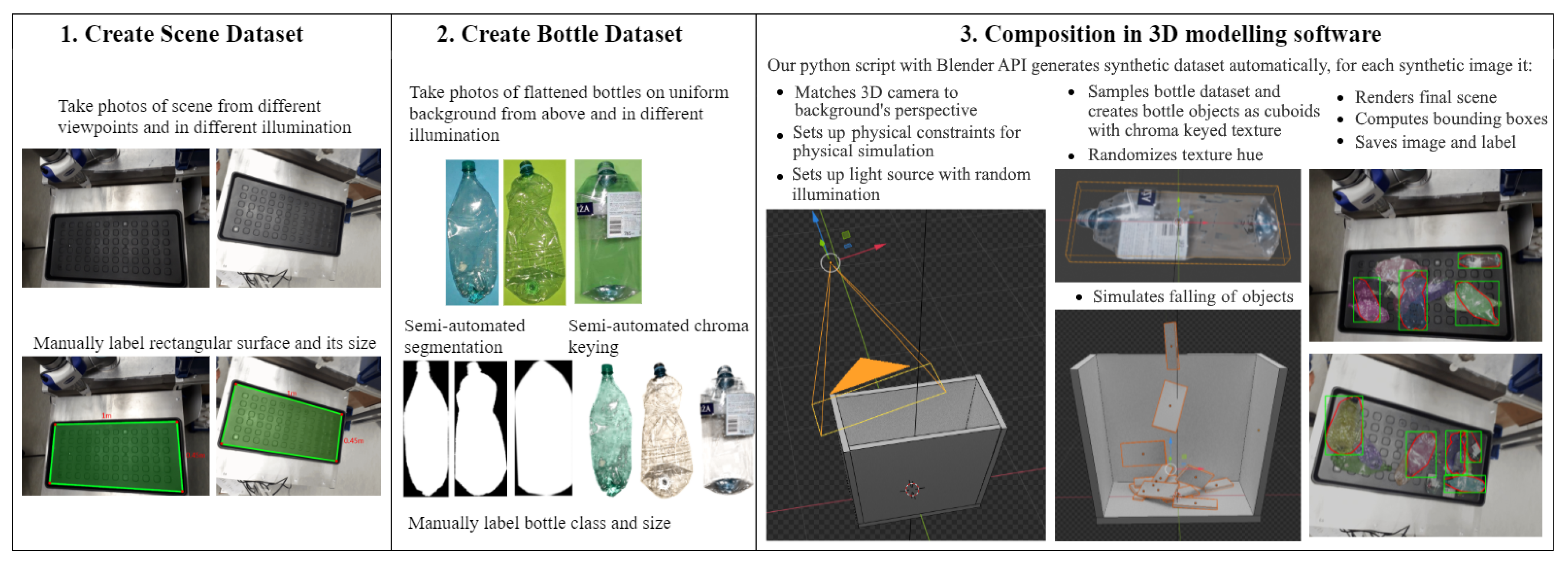
Similar to the synthetic data generation pipelines proposed in [13,14,15], we developed a synthetic data generation pipeline tailored for the task of visually recognizing piles of plastic bottles. For 3D physics and rendering engine, we uses the open-source Blender 3D creation suite [16], which provides Python API that allows automating virtual scene construction and rendering. We reconstructed a virtual environment from 2D photos of the scene containing a rectangular planar surface. Due to notable difficulty in 3D scanning of transparent objects, we only reconstructed bottles as planar objects with the 2D texture of real bottles. This solution does not harm our application as plastic bottles are expected to be crushed, i.e., flattened; however, for undeformed bottles, a camera can be placed above the scene. An overview of our proposed pipeline is given in Figure 1. The proposed data generation methodology can also be applied to different kinds of objects and materials as long as 3D models of objects of interest are available. The code and data for the synthetic data generator and for reproducing all results are availableat https://pubgit.edi.lv/vitalijs.fescenko/synthetic-data-for-pet-bottle-detection, accessed on 19 October 2022.
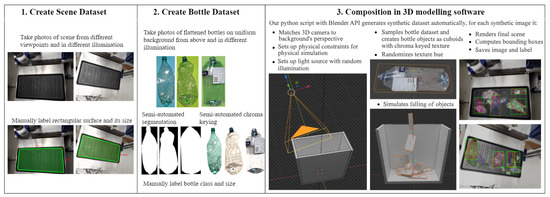
Figure 1.
Proposed approach of generating synthetic data for detecting transparent bottles in piles.
The contribution of our work consists of:
- Photo-realistic synthetic data generation pipeline tailored to the task of visually detecting piles of flattened plastic multi-class bottles.
- Detailed quality evaluation of the generated synthetic data against a real dataset gathered in a conventional way by comparing the performance of object detection in both cases.
The rest of this paper is organized as follows: Section 2 reviews related works on synthetic data generation and object detection. Section 3 describes our methodology of generating synthetic data as well as the collection of real data. Experimental results are shown and discussed in Section 4. Section 5 gives the conclusion.
2. Related Work
2.1. Object Detection
Object detection is one of the main computer vision tasks and refers to the identification and localization of objects in images or videos, with a wide range of applications such as medical diagnosis systems, video analysis and monitoring systems and autonomous robotic systems.
Nowadays, artificial neural networks (ANN) prevail in object detection tasks due to state-of-the-art performance of classical CNN methods, such as Fast R-CNN [17], Faster R-CNN [18], YOLO family [19,20,21,22,23] and SSD [24], as well as more recent EfficientDet [25] and visual transformer methods, such as DETR [26].
The YOLO family of object detectors is known for a good trade-off between performance and speed when compared to other methods. According to [19], YOLO performs slightly worse than Fast R-CNN and Faster R-CNN on the PASCAL VOC dataset while performing significantly faster. YOLOv3 performs similarly to SSD on MS COCO, while performing three times faster [21]. More recent YOLO incarnations include YOLOv4 [22] and Ultralytics’ “YOLOv5” repository [23].
In this paper, we use the “YOLOv5” repository as it is implemented in PyTorch, thus simplifying experimentation, deployment and re-training of the object detector. Moreover, YOLOv3 has already been successfully applied to PET bottle detection on conveyor belts and classification by colour [12], proving the applicability of YOLO detectors for a similar task.
2.2. Synthetic Data
Synthetic data are a tempting alternative to manual collection on a large scale due to the ease of data generation after an initial effort to set up the generator. The goal is to generate synthetic data that generalizes to the real domain.
In visual object detection tasks, synthetic data consist of images generated by placing foreground objects on background scenes, i.e., composition, with an additional variation, such as change of object and camera position, illumination, object texture and shape. Object placing can be random, using out-of-context backgrounds [27,28,29], with additional contextual guidance [30,31] or realistic placing using rules or physical simulation [13,15,32,33].
Methods, such as [27,28,30], use 2D cut-and-paste techniques for data generation, where objects are cut from images and placed on top of a separate set of background images. In [30], the authors used pre-made datasets of segmented objects; Ref. [28] used computer vision algorithms for segmentation, while [27] trained a dedicated segmentation model. Similar methods are only suitable for generation of 2D labels, such as bounding boxes or segmentation mask; however, they are often simpler in terms of complexity and data acquisition.
With the availability of large datasets of 3D CAD models, such as “3D Warehouse” (3D CAD model warehouse: https://3dwarehouse.sketchup.com/, accessed on 19 October 2022) and ShapeNet [34], datasets of 3D scanned models [35] and advances in computer graphics, recent work in synthetic data [13,14,15,31,32,36,37] has shifted to 3D graphical engines that allow easy integration of 3D background scenes and 3D objects, enabling more variation and more realistic scene reconstruction and object placement. Some work uses pre-made 3D background scenes [13,14], while others use complex 3D scanning techniques to recreate the target environment [15]. Older methods use 2D background images for 3D object placement [31]; however, additional scene analysis or manual labelling is required for realistic object placement. Objects can also be taken from pre-made datasets [13,14,29,31] and reconstructed either manually [32] or by scanning real objects for more realism [15].
For a custom task, the reuse of pre-made datasets might not be possible. Thus, similar to [15,27], our work presents a full pipeline of collecting objects and backgrounds as well as a method that allows generating an object detection dataset for a cluttered scene. However, our solution is tailored more to the detection of flat transparent objects, such as crushed plastic bottles. We use photos of backgrounds and bottles. We follow a realistic object placement approach by reconstructing a virtual 3D scene in Blender from a background photo using a rectangular surface and performing a 3D physics simulation.
Most recent work on synthetic data either train models on generated data exclusively [28,29,32,38] or simply merge real and generated datasets in some proportions due to superior performance [13,14,15,27,39]. However, it might introduce bias in favour of synthetic data due to larger dataset size. Therefore, we propose to use a multi-task [40] inspired loss function that views synthetic and real datasets as equal tasks and balances their contribution by weighting respective gradients.
3. Methods
3.1. Synthetic Data Generation
Our proposed synthetic dataset generation approach can be summarized as follows. First, we collect and label datasets of background and bottle photos. Then, we generate synthetic data in a 3D modelling software by reconstructing a virtual environment from the background photos, reconstructing bottle objects from the bottle photos, simulating cluttering of the bottle objects and render the final scene with bounding box labels. An overview of our approach is given in Figure 1.
3.1.1. Background Dataset Creation
A background dataset is required for the composition of backgrounds and foreground objects. We further describe our approach to collecting and processing backgrounds.
Collecting background scene photos: We take different photos of the same scene from above with slight variations in perspective and illumination. This camera placement provides the best visibility of flattened bottles and enables the use of undeformed bottles. We limit photos to just one scene, which consists of an experimental setup of a table with a robot arm attached and a rectangular plastic tray for placing bottles; however, our approach can also be used with multiple scenes, assuming they all contain planar rectangular surfaces such as a tabletop, conveyor belt or a floor.
Labelling: The label for each photo consists of the dimensions and corner points of the rectangular surface. This information is necessary for a realistic up-to-scale virtual scene reconstruction described in Section 3.1.3. Label calculation can be automated using pose estimation of fiducial markers, e.g., Aruco markers [41].
The described background dataset creation approach is simple for the end user, as it only requires a photo from the desired viewpoint and a label, while not requiring any 3D software knowledge or a complex pipeline for the 3D scene reconstruction. However, the main drawback is object placement only in a predefined region with predefined physical constraints.
3.1.2. Bottle Dataset Creation
For foreground objects, we collect, scan and process transparent bottles in a specific way suitable for the proposed synthetic data pipeline.
Collecting bottle instances and photos: We collected 136 PET bottles of common beverages and bottled water. Bottles were manually flattened to correspond to expected conditions. Then, for each bottle instance, we took multiple photos at varying illumination from different flat sides on a uniform background. The colour of the background should not be included in the object for proper post-processing described later in this paper. We mostly used green and blue backgrounds.
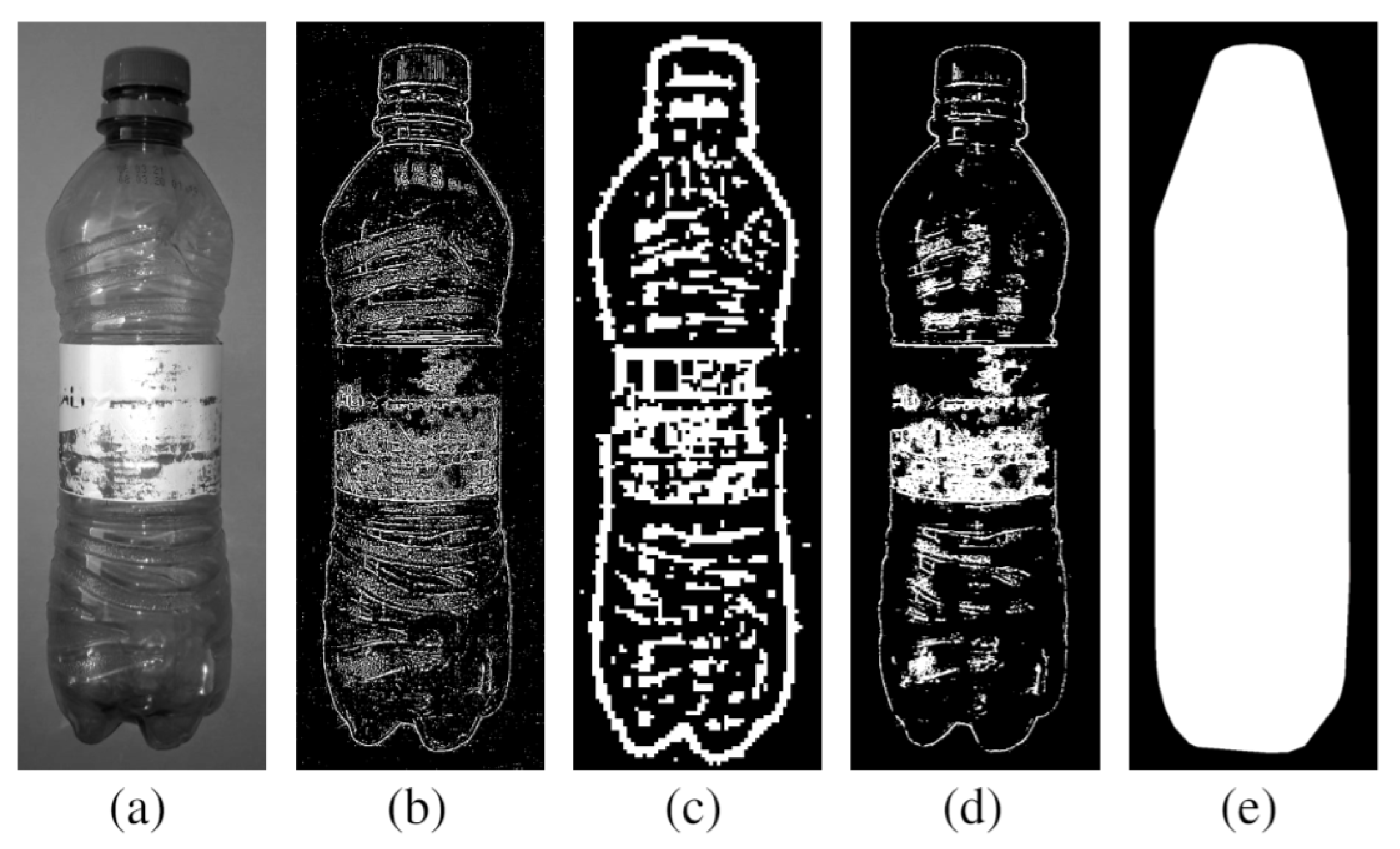
Segmentation: Segmentation is necessary for bottle localization in a photo and for establishing a hard boundary. For this purpose, we developed a GUI Python application using OpenCV [42] computer vision library. Clear separation of a background from a bottle by intensity threshold is not always possible due to transparency and varying colours of the background; thus, we used an edge-based method that we empirically found to work well for transparent bottles on a uniform background (Figure 2a). For our segmentation method, we used Laplacian pyramid [43] which acts as a band-pass filter for certain frequency features. The first layer keeps only high-frequency features, such as edges or noise, while the last layer keeps lower-frequency features. We converted both layers to binary images (Figure 2b,c) and performed a pixel-wise AND binary operation (Figure 2d) to leave only pronounced edges while filtering out noise. The user of our application is required to eyeball the depth of a pyramid, such that only noise is filtered, while enough edges are preserved. Then, in case of a discontinuity of the object’s edges, we compute a convex hull from all remaining edges (Figure 2e). Convex hull preserves the bounding box of an object, which suits our task of object detection; however, for the segmentation task, additional effort would be required for computing a more precise boundary.
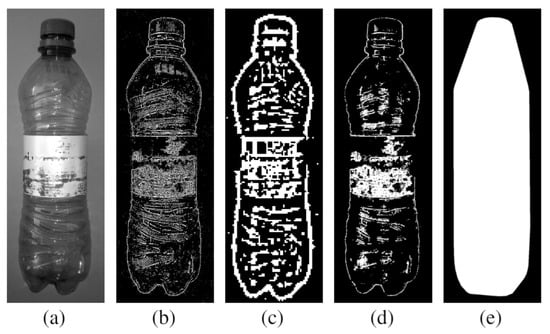
Figure 2.
Bottle segmentation steps (left to right): (a) input grayscale image; (b) binary first Laplacian pyramid layer; (c) binary last (4th) Laplacian pyramid layer; (d) pixel-wise AND of (b,c); (e) convex hull.
Image matting: The extraction of opacity information of a foreground object, such as a bottle, from an image is known as image matting. We use Blender’s implementation of the image matting algorithm by chroma keying [44] designed to work with transparent or translucent objects. We wrap it in a Python script that accepts the image and chroma key the RGB value as arguments. The chroma key value is calculated as an average intensity of a background. However, we found that the results of this algorithm depend on the background illumination and can leave part of the background translucent. This can be mitigated to some extent by masking the result with a segmentation mask or selecting a better chroma key value. For this reason, we do not consider this step to be fully automated yet, and further research into better image matting methods should be conducted.
Labelling: We manually label bottle size and class for each bottle instance. In this paper we consider four classes determined by the presence of a cap or a label: both present, only cap, only label and none. Approximate bottle size can also be computed automatically knowing the pixel/centimetre ratio.
Overall, this approach could be simple for the end user, assuming less manual intervention in image matting and segmentation would be required. In comparison with the conventional labelling approach, where the amount of labels required is equal to the total occurrences of objects in all images, our method only requires a label for each object instance.
3.1.3. Composition
We create a Python script with the Blender-API that automatically generates a synthetic dataset. For each synthetic image, it performs the composition of background scenes and bottles inside Blender. For composition, we introduce multiple simulated sources of variation, namely the bottle’s colour, hue and size variations, scene illumination and an amount of uniquely cluttered scenes per dataset as a way to augment the dataset and deal with missing or imprecise information, as well as to make our detector robust against small changes in terms of variation. This approach, although on a smaller scale, follows a similar principle to domain randomization [32], namely extensive simulation of variation in the hope of also covering the real domain. We further describe our composition script and its key steps.
Scene reconstruction: Our script launches Blender software and loads a random background photo from the background dataset described in Section 3.1.1. It matches the perspective and scale of a background to a virtual 3D camera object using a Blender add-on for camera calibration [45], which uses perspective views of rectangles for estimating camera position based on the algorithm introduced in [46]. Then, our script sets up a physical constraints box that prevents objects from falling outside the labelled rectangular surface. We do not reconstruct correct illumination as it is challenging to extract from a single photo; instead, our script creates a 3D light object with varying softness and brightness.
Loading bottles: Next, our script samples a few bottle instances from the bottle dataset described in Section 3.1.2 and for each bottle loads its dimensions, chroma-keyed textures and segmentation masks. For each sampled bottle instance, the script creates a 2D rectangular object that matches the real-life size and randomly samples one of the bottle’s chroma-keyed photos to use as the bottle object’s texture. For physical simulation stability, an additional thin 3D bounding box is created around each bottle object. All bottle objects are stacked vertically without overlap on top of a constraints box. For each synthetic image, the rotation and position of bottle objects and their hue and size. The number of bottles to load is varied. We also vary the amount of uniquely cluttered scenes per dataset; namely, we either select bottles randomly for each scene in the dataset or repeat one bottle selection in multiple scenes.
Simulation and rendering: Cluttering is achieved by applying a force of gravity to bottle objects and running a physical simulation during which objects fall inside the constraints box. After simulation, our script renders and saves the final scene using Blender’s Cycles physically based rendering engine.
Label generation: Our final goal is to acquire bounding box labels for unobstructed, i.e., topmost bottles, which represent pickable bottles. For this task, each bottle’s outline is computed from the segmentation mask and is projected onto the camera’s image plane. Then, using the Python Shapely library [47] for manipulation and analysis of planar geometric objects, overlapping bottles are determined via intersection over union (IOU) between their outlines. Bottles that do not overlap are considered unobstructed, while for overlapping pairs we determine the topmost bottle by comparing their altitude in a simulated environment with respect to the virtual camera. Finally, bounding boxes of the unobstructed bottles are computed and exported to the YOLO label format.
3.2. Datasets
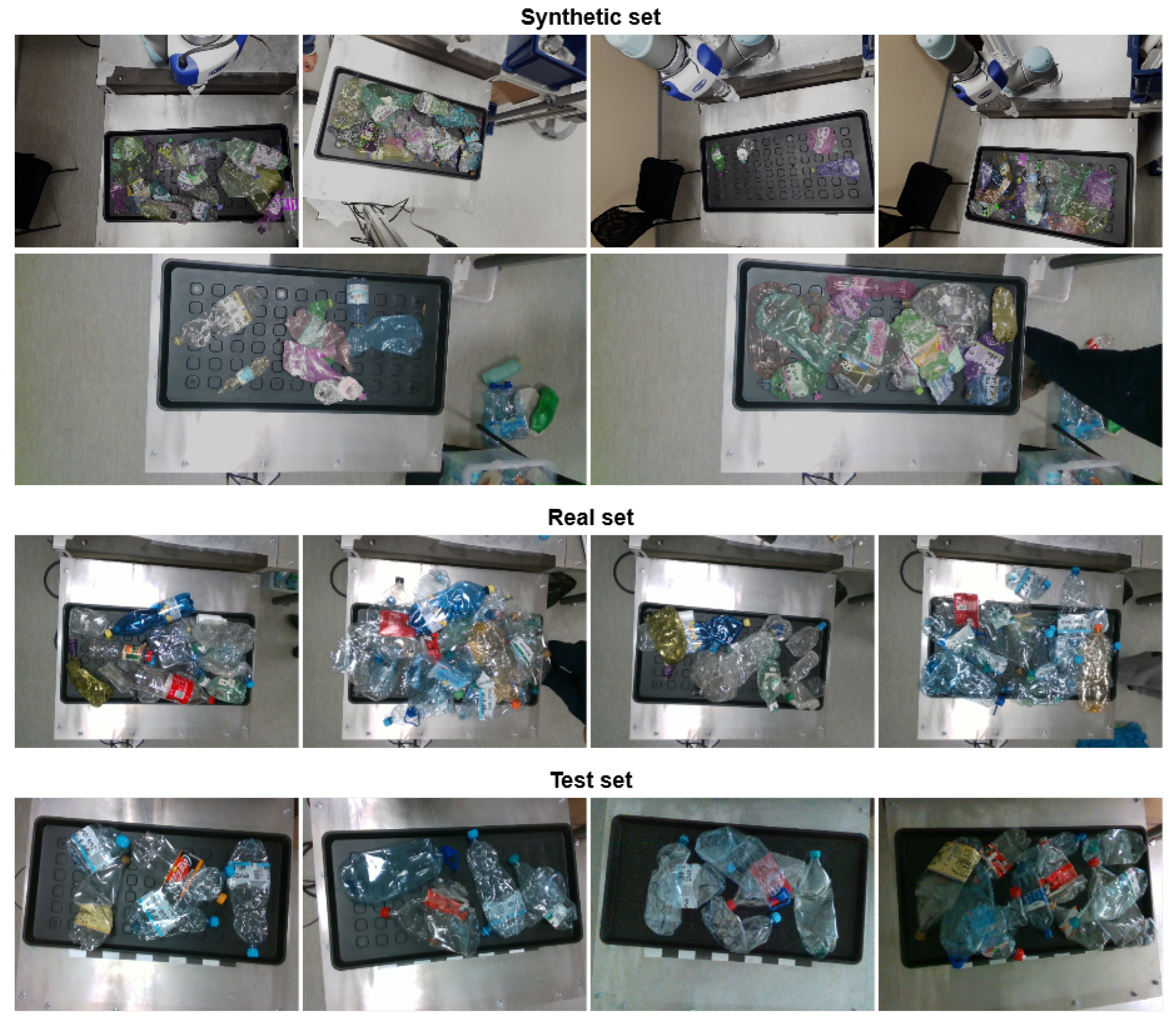
We further describe synthetic and real datasets we have collected for training object detectors in multiple scenarios. See Figure 3 for samples from those datasets.

Figure 3.
Samples from different datasets. For the synthetic set, we show samples generated using all sources of variation.
3.2.1. Synthetic Datasets
Using the approach described in Section 3.1, we generated several synthetic datasets with various sources of variation consisting of 5000 images each. Unless stated otherwise, we use synthetic data with all sources of variation enabled. We use 80% for training and the rest for validation.
3.2.2. Real Datasets
Real data were collected in the same environment described in Section 3.1.1. We manually clutter the plastic tray on the table with the same bottles used in synthetic dataset generation and take photos with a camera mounted above. Then, with the help of our colleagues, we manually labelled bounding boxes and classes.
Real set: We denote a real set as data collected for training and validation. It consists of 2031 photos taken in bright illumination from a single viewpoint and with a small amount of uniquely cluttered scenes, where in-between photos capture the consecutive addition or removal of a few bottles from the tray, which yields significant overlap in nearby photos in terms of pixel values. We split the dataset consecutively using the first 80% of photos for training and the rest for validation, as we found random splitting harms generalization due to overlap in training and validation sets. While this data collection method does not fully represent our target domain as it contains a smaller amount of variation than we expect our object detector to cover, it is easier to manually collect and label data in this way in the real environment, where regular retraining is expected.
Test set: The test set consists of real data that captures all the variation we expect from a good object detector to cover, in other words, it represents our target domain. It consists of 51 uniquely cluttered scenes with 3 illumination conditions (bright lamp, dim lamp, ambient light) and 4 camera positions from above, 612 images in total.
3.3. Object Detector
For all experiments, we use Ultralytics “YOLOv5” object detector, specifically the smallest architecture available named “YOLOv5s” with weights pre-trained on ImageNet. All size models use the same architecture with the only difference being depth and width scaling factors, which add more layers in-depth or add more parameters at each layer, respectively.
For each prediction, “YOLOv5” outputs bounding box coordinates and confidence and classification score. Similarly to YOLOv3, class probabilities and confidence are computed using independent logistic classifiers. Confidence, i.e., objectiveness, score is trained to have a value of 1 if the predicted bounding box overlaps best with ground truth. During prediction, confidence is used as a proxy for assessing the quality of the predicted bounding box. Similarly to YOLOv3, “YOLOv5” predicts bounding box coordinates as for the top-left corner and for dimensions; however, the formula used to convert the output into bounding box coordinates slightly differs to improve stability during training:
where is the anchor’s width and height, is the anchor’s offset from the top left corner of the image, are predicted offsets with regard to the anchor’s position, and are predicted scaling ratios with regard to the anchor’s dimensions. Anchors are computed by clustering bounding boxes in a dataset using k-means. “YOLOv5” by default uses anchors pre-trained on the MS COCO dataset adopted from [21].
For evaluation of the object detector, we use the mAP@0.5:0.95 performance metric implementation provided in “YOLOv5” based on code from [48] that uses a 101-point interpolation for precision × recall curve approximation. The mean average precision (mAP) metric is often used for the evaluation of object detectors’ performance in competitions; mAP is computed as the mean of average precision (AP) scores per object class. The standard AP metric considers the predicted bounding box as true positive if it overlaps with ground truth by at least 50% from their total covered area, i.e., their intersection over union (IOU) threshold is 50%. The mAP@0.5:0.95 computes the mean value of 10 mAP scores with IOU thresholds varying in a range of 50% to 95% with steps of 5% [48]. In contrast to standard mAP, the mAP@0.5:0.95 metric better depicts the localization precision of predicted bounding boxes.
3.4. Training
We train all models using default hyper-parameters and configuration in the “YOLOv5” implementation, namely 300 training epochs, mini-batch gradient descent with Nesterov momentum of 0.937 [49] and mini-batch size of 32 images, weight decay, cosine learning rate decay strategy [50] from 0.01 to 0.002 at the final epoch and a learning rate and momentum warmup heuristic [50] for 3 initial epochs. For image augmentations, “YOLOv5” by default uses mosaic augmentation [22], random HSV colour space adjustment and horizontal flip. For evaluation on the test set, we only select the best weights among all epochs in terms of mAP@0.5:0.95 performance on the respective validation set.
During experiments, we train multiple object detector model variants. For each model variant, we trained 6 models in order to reduce noise in the results. We measure mAP@0.5:0.95 metrics on the test set.
We further refer to models trained on either synthetic or real datasets as single dataset models or synthetic and real models, respectively. For models trained on both synthetic and real datasets, we refer to them as either concatenated or combined models depending on the method (see further discussion).
Concatenated model: The simplest way of combining two datasets is to merge, i.e., concatenate, train sets and validations, sets respectively. We trained two concatenated model variants. The first variant validates on concatenated validation sets from both datasets. The second one only validates on a real validation set, but due to similar performance and for a fair comparison with the combined models (explained in the next paragraph), we only report the latter model.
Combined model: Synthetic data are usually more abundant than real data. Thus, simply merging both datasets “synthetic” gradient can suppress the “real” gradient during optimization. We use a multi-task-inspired loss function to balance the contribution of “real” and “synthetic” gradients. More specifically, we scale the “YOLOv5” mini-batch loss using the following expression:
where and denote synthetic and real training sets, respectively, B is a mini-batch sampled from either set, and is an additional scaling parameter that weights the contribution of each set to the gradient. In experiments, we use for equal contribution unless stated otherwise. A bigger value means a larger real set contribution, while a smaller value means a larger synthetic set contribution. We save best weights by only validating on a real validation set as it facilitates our goal to generalize the detector to a real domain and frees us from additionally weighting validation performance on both sets.
4. Results
We perform multiple experiments in order to evaluate our generated data against data collected in a conventional way.
4.1. Synthetic Data versus Real
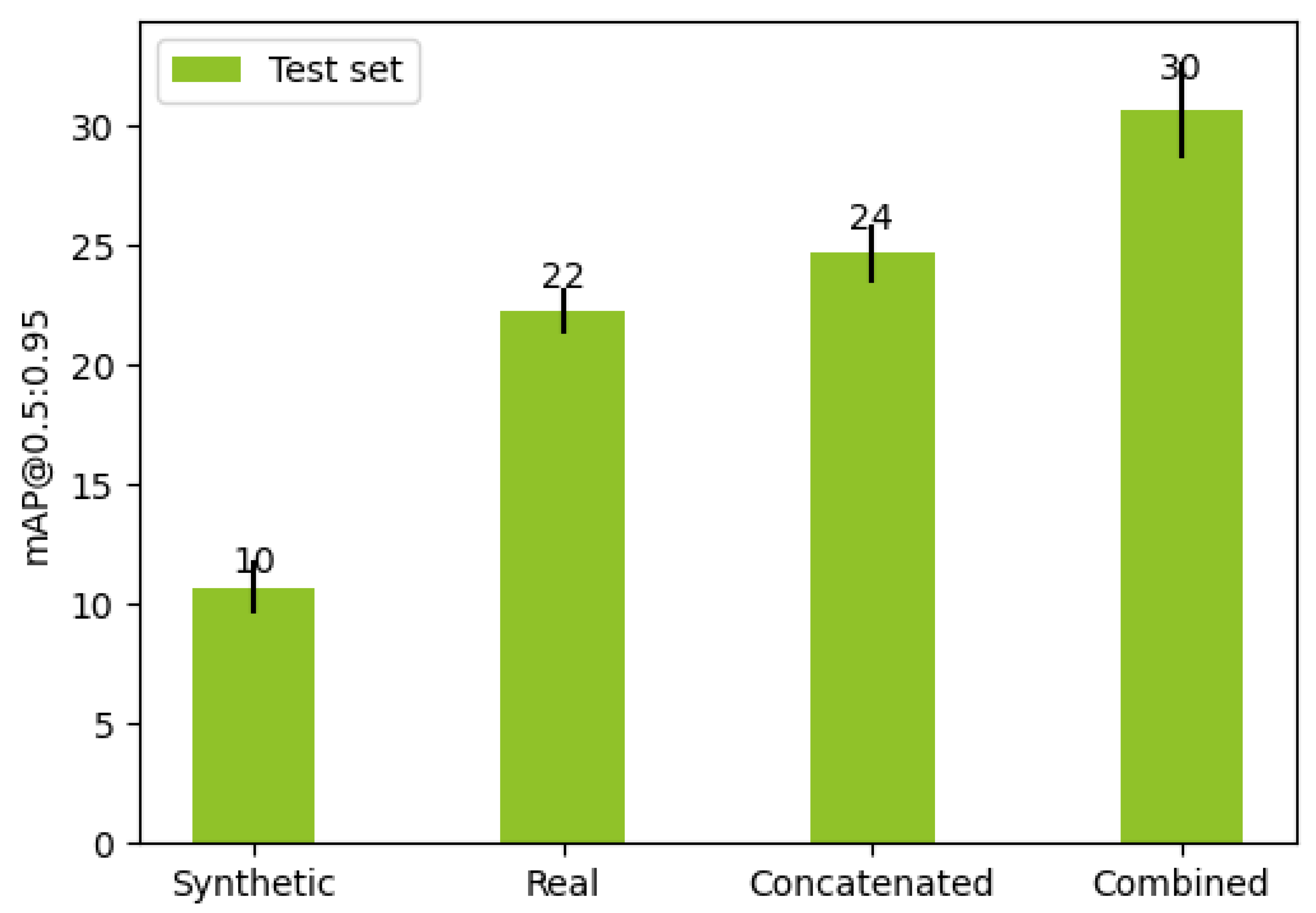
First, we compare the performance of models trained on real, synthetic and combined datasets. Figure 4 shows the results of our experiment.
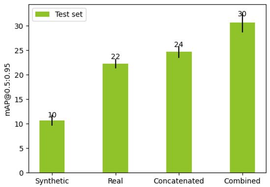
Figure 4.
Average performance of models. Lines represent one standard deviation.
Results show that models that use a combination of synthetic and real data perform better on average. Combined models on the test set achieved 30 mAP@0.5:0.95 on average which is 1.36 times more than real models and 1.25 times more than concatenated.
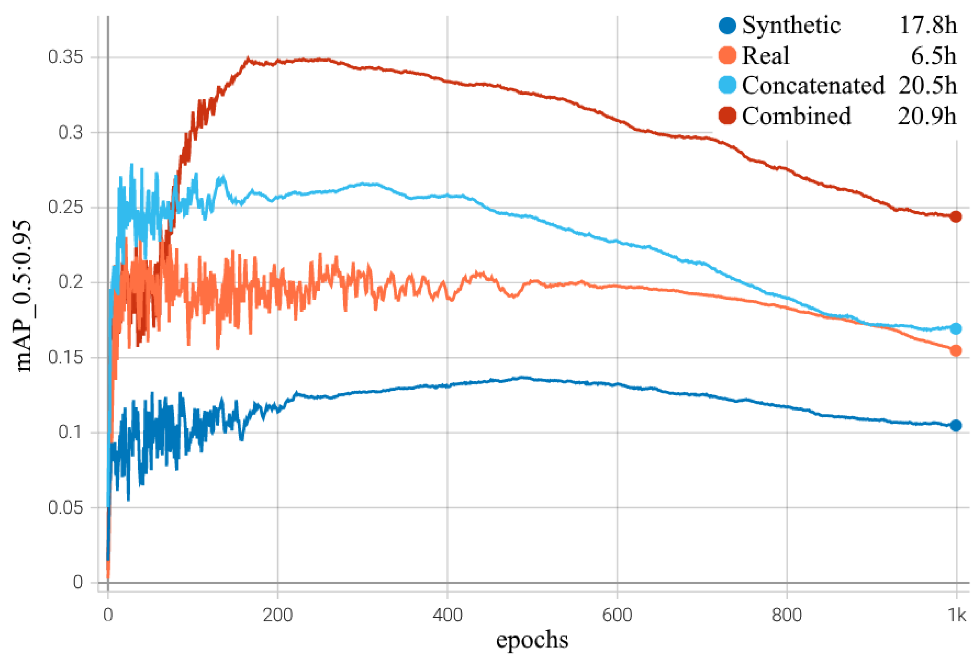
We perform an additional experiment to confirm that the worse performance of single dataset models on the test set is not caused by smaller datasets, i.e., fewer mini-batch weight updates. Combined and concatenated models use 5624 training images, thus having 176 mini-batches per epoch or 52,800 for 300 epochs. Synthetic models have 125 mini-batches per epoch, and real models have 51. Thus, for an equal number of weight updates, synthetic and real models should train for 423 and 1035 epochs, respectively. We train each model variant for 1000 epochs and plot performance on the test set for each epoch (see Figure 5). As can be seen from the figure, even at a similar number of weight update steps, the performance of the synthetic and real models is similar to that reported in Figure 4 and becomes worse due to overfitting.
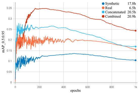
Figure 5.
Test performance with respect to epochs with time measured on Nvidia Quadro RTX 4000.
4.2. Ablation Study
To study the significance of the simulated variation in the synthetic data, we perform an ablation study by restricting some sources of variation during data generation. Sources of variations we explore are random colour (hue), multiple camera viewpoints, random illumination, multiple photos for each bottle and the amount of uniquely cluttered scenes. To remove the variation introduced from multiple camera viewpoints or bottle photos, we restrict backgrounds to one viewpoint and bottles to one photo. To remove random illumination, we fix Blender’s light object to one position and brightness. To reduce the variation from uniquely cluttered scenes, we use only 50 unique bottle selections per dataset. For each synthetic dataset variant, we train both the synthetic and combined models. Table 1 summarizes our results.

Table 1.
Ablation studies on the sources of variation in the synthetic dataset. We generate various synthetic datasets by restricting one or more sources of variation and evaluate the performance of models trained on these datasets.
For the synthetic-only models, results show that all sources of variation except for uniquely cluttered scenes improve performance. The most significant sources of variations are multiple photos of each bottle and random colours. Uniquely cluttered scenes harm the performance.
For the combined dataset models, only multiple camera viewpoints and multiple photos of each bottle provide significant improvement. Uniquely cluttered scenes and random colour harm the performance.
Overall, results suggest that variation plays an important role in generalization, especially in the synthetic-only models. Using multiple photos of each bottle significantly improves the performance; however, such variation is manually collected rather than simulated. Among simulated variation, randomization of bottles’ colour provides improvement when trained without real data, while slightly harming performance in combination with real data. Randomization of illumination in a simulated environment tends to slightly improve performance on the target domain. Using a unique selection of bottles per scene hurts the performance as reusing the same bottle selection performs better; however, we do not explore this phenomenon further.
4.3. Comparison of Dataset Sizes
In order to find out whether the combined model’s performance could be traded away in favour of a smaller real dataset size, we experiment with different sizes. We divide the real dataset into three subsets, namely 25%, 50% and 75%, by taking only the corresponding percentage of data from the beginning of the full dataset for both training and validation sets. We additionally train the real models on those subsets to confirm that reducing data reduces performance, which might not be the case if images contained a lot of redundant information due to overlap. For the combined models, we use a full synthetic dataset. Table 2 summarizes our results.

Table 2.
Performance (mAP@0.5:0.95) with respect to real dataset size.
The best results are achieved by the combined models trained on 100% of real data. The combined models with only 25% of real data achieve a similar performance to the real models on the test set, which suggests that in our case the amount of real data can be reduced by a factor of four if trained in combination with synthetic data. However, for the validation set, only 25% of the real data can be removed without performance loss.
4.4. Contribution of Datasets
We perform additional tests to find an optimal contribution ratio between synthetic and real training sets, more specifically we train combined models with multiple values in the combined loss (Equation (2)). A bigger value means more real set contribution, while a smaller value means more synthetic set contribution. For models with we reuse combined models from previous experiments, while and models, corresponding to the real and synthetic models, respectively, are trained from scratch due to minor differences from using combined loss. Results are summarized in Figure 6.
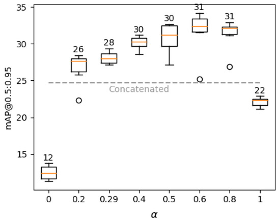
Figure 6.
Box plot of the combined models with respect to alpha values in combined loss. Average performance is shown above the boxes. Grey dashed line represents average performance of the concatenated models.
Models with ranging from 0.4 to 0.8 achieve good results with minor differences; however, favouring real data slightly more () gives the best result. By favouring synthetic data four times more (), we obtain worse results than by favouring real data by the same amount (), confirming the real data is more important. As expected, models score similar performance to their regular loss function analogues (see Figure 4); however, both are outperformed by models, suggesting that even a small contribution from an opposite set significantly improves performance.
By simply merging both datasets, performance should be close to models due to having a proportion of real training data among the whole concatenated training set. However, surprisingly, we observed worse performance for concatenated models, which might be caused by different loss scales due to the use of combined loss. Nevertheless, even models perform worse than by favouring real data, confirming that balancing the contribution of datasets is useful when using larger synthetic datasets.
5. Conclusions
We show promising results that the proposed synthetic data generation method can be used for the visual detection of transparent bottles. From our results, we conclude that generated synthetic data are not a good replacement for real data on its own due to worse performance; however, it can provide additional information due to the vast amount of variations. We also show that in our case, synthetic data can substitute 75% of real data without performance loss, suggesting our generator could ease data collection under the assumption that preparing datasets for the generator will become more automated.
We also show that balancing both datasets achieves performance 1.36 times better than models trained only on real data and 1.25 times better than by simply merging both datasets. We also show the importance of amplifying real dataset gradient during training for better generalisation to the real target domain, which cannot be achieved by simply merging both datasets if synthetic data is more abundant.
Thus, future work includes fully automating our proposed pipeline, specifically segmentation and chroma keying steps, and bridging the gap between real and synthetic domains.
Author Contributions
Conceptualization, V.F., R.K. and J.Ā.; methodology, V.F. and J.Ā.; software, V.F.; validation, V.F.; formal analysis, V.F.; investigation, V.F.; resources, R.K. and V.F.; data curation, V.F., J.Ā. and R.K.; writing—original draft preparation, V.F. and J.Ā.; writing—review and editing, V.F., R.K. and J.Ā.; visualization, V.F.; supervision, R.K.; project administration, R.K.; funding acquisition, R.K. All authors have read and agreed to the published version of the manuscript.
Funding
This work has received funding from Latvian state budget under agreement No ES RTD/2021/13, H2020 ECSEL Joint Undertaking project IMOCO4.E under grant agreement No 101007311, and H2020 ESCEL Joint Undertaking project VIZTA under grant agreement No 826600.
Institutional Review Board Statement
Not applicable.
Informed Consent Statement
Not applicable.
Data Availability Statement
The data presented in this study are openly available in our repository at https://pubgit.edi.lv/vitalijs.fescenko/synthetic-data-for-pet-bottle-detection (accessed on 29 December 2022).
Conflicts of Interest
The authors declare no conflict of interest.
References
- Torres, P.; Arents, J.; Marques, H.; Marques, P. Bin-Picking Solution for Randomly Placed Automotive Connectors Based on Machine Learning Techniques. Electronics 2022, 11, 476. [Google Scholar] [CrossRef]
- Čech, M.; Beltman, A.J.; Ozols, K. Digital Twins and AI in Smart Motion Control Applications. In Proceedings of the 2022 IEEE 27th International Conference on Emerging Technologies and Factory Automation (ETFA), Stuttgart, Germany, 6–9 September 2022; pp. 1–7. [Google Scholar]
- Arents, J.; Greitans, M. Smart Industrial Robot Control Trends, Challenges and Opportunities within Manufacturing. Appl. Sci. 2022, 12, 937. [Google Scholar] [CrossRef]
- Racinskis, P.; Arents, J.; Greitans, M. A Motion Capture and Imitation Learning Based Approach to Robot Control. Appl. Sci. 2022, 12, 7186. [Google Scholar] [CrossRef]
- Russakovsky, O.; Deng, J.; Su, H.; Krause, J.; Satheesh, S.; Ma, S.; Huang, Z.; Karpathy, A.; Khosla, A.; Bernstein, M.; et al. ImageNet Large Scale Visual Recognition Challenge. Int. J. Comput. Vis. (IJCV) 2015, 115, 211–252. [Google Scholar] [CrossRef]
- Everingham, M.; Gool, L.; Williams, C.K.I.; Winn, J.; Zisserman, A. The Pascal Visual Object Classes (VOC) Challenge. Int. J. Comput. Vis. 2009, 88, 303–338. [Google Scholar] [CrossRef]
- Lin, T.Y.; Maire, M.; Belongie, S.; Hays, J.; Perona, P.; Ramanan, D.; Dollár, P.; Zitnick, C.L. Microsoft COCO: Common Objects in Context. In Proceedings of the Computer Vision— ECCV 2014; Fleet, D., Pajdla, T., Schiele, B., Tuytelaars, T., Eds.; Springer International Publishing: Cham, Switzerland, 2014. [Google Scholar]
- Bobulski, J.; Piatkowski, J. PET Waste Classification Method and Plastic Waste DataBase–WaDaBa. In Proceedings of the Image Processing and Communications Challenges 9; Choraś, M., Choraś, R.S., Eds.; Springer International Publishing: Cham, Switzerland, 2018; pp. 57–64. [Google Scholar] [CrossRef]
- Thung, G.; Yang, M. Trashnet Dataset for Garbage Classification. 2016. Available online: https://github.com/garythung/trashnet (accessed on 20 October 2022).
- Proença, P.F.; Simões, P. TACO: Trash Annotations in Context for Litter Detection. arXiv 2020, arXiv:2003.06975. [Google Scholar] [CrossRef]
- Lai, Y.L.; Lai, Y.K.; Shih, S.Y.; Zheng, C.Y.; Chuang, T.H. Deep-learning Object Detection for Resource Recycling. J. Phys. Conf. Ser. 2020, 1583, 012011. [Google Scholar] [CrossRef]
- Jeon, Y.; Um, S.; Yoo, J.; Seo, M.; Jeong, E.; Seol, W.; Kang, D.; Song, H.; Kim, K.S.; Kim, S. Development of real-time automatic sorting system for color PET recycling process. In Proceedings of the 2020 20th International Conference on Control, Automation and Systems (ICCAS), Busan, Republic of Korea, 13–16 October 2020; pp. 995–998. [Google Scholar] [CrossRef]
- Rajpura, P.S.; Bojinov, H.; Hegde, R.S. Object Detection Using Deep CNNs Trained on Synthetic Images. arXiv 2017, arXiv:1706.06782. [Google Scholar] [CrossRef]
- Tremblay, J.; To, T.; Sundaralingam, B.; Xiang, Y.; Fox, D.; Birchfield, S. Deep Object Pose Estimation for Semantic Robotic Grasping of Household Objects. arXiv 2018, arXiv:1809.10790. [Google Scholar]
- Wang, K.; Shi, F.; Wang, W.; Nan, Y.; Lian, S. Synthetic Data Generation and Adaption for Object Detection in Smart Vending Machines. arxiv 2019, arXiv:1904.12294. [Google Scholar] [CrossRef]
- Blender Online Community. Blender—A 3D modelling and rendering package (Version 2.80); Blender Foundation, Stichting Blender Foundation: Amsterdam, The Netherlands, 2019; Available online: http://www.blender.org (accessed on 20 October 2022).
- Girshick, R.B. Fast R-CNN. In Proceedings of the 2015 IEEE International Conference on Computer Vision (ICCV), Santiago, Chile, 7–13 December 2015; pp. 1440–1448. [Google Scholar] [CrossRef]
- Ren, S.; He, K.; Girshick, R.; Sun, J. Faster R-CNN: Towards Real-Time Object Detection with Region Proposal Networks. IEEE Trans. Pattern Anal. Mach. Intell. 2017, 39, 1137–1149. [Google Scholar] [CrossRef] [PubMed]
- Redmon, J.; Divvala, S.; Girshick, R.; Farhadi, A. You Only Look Once: Unified, Real-Time Object Detection. In Proceedings of the 2016 IEEE Conference on Computer Vision and Pattern Recognition (CVPR), Las Vegas, NV, USA, 27–30 June 2016; pp. 779–788. [Google Scholar] [CrossRef]
- Redmon, J.; Farhadi, A. YOLO9000: Better, Faster, Stronger. arXiv 2016, arXiv:1612.08242. [Google Scholar] [CrossRef]
- Redmon, J.; Farhadi, A. YOLOv3: An Incremental Improvement. arXiv 2018, arXiv:1804.02767. [Google Scholar] [CrossRef]
- Bochkovskiy, A.; Wang, C.Y.; Liao, H.Y.M. YOLOv4: Optimal Speed and Accuracy of Object Detection. arXiv 2020, arXiv:2004.10934. [Google Scholar] [CrossRef]
- Jocher, G. Ultralytics “YOLOv5”. 2020. Available online: https://github.com/ultralytics/yolov5 (accessed on 20 October 2022).
- Liu, W.; Anguelov, D.; Erhan, D.; Szegedy, C.; Reed, S.; Fu, C.Y.; Berg, A.C. SSD: Single Shot MultiBox Detector. In Proceedings of the Computer Vision—ECCV 2016; Leibe, B., Matas, J., Sebe, N., Welling, M., Eds.; Springer International Publishing: Cham, Switzerland, 2016; pp. 21–37. [Google Scholar]
- Tan, M.; Pang, R.; Le, Q.V. EfficientDet: Scalable and Efficient Object Detection. In Proceedings of the 2020 IEEE/CVF Conference on Computer Vision and Pattern Recognition (CVPR), Seattle, WA, USA, 13–19 June 2020; pp. 10778–10787. [Google Scholar] [CrossRef]
- Carion, N.; Massa, F.; Synnaeve, G.; Usunier, N.; Kirillov, A.; Zagoruyko, S. End-to-End Object Detection with Transformers. In Proceedings of the Computer Vision—ECCV 2020; Vedaldi, A., Bischof, H., Brox, T., Frahm, J.M., Eds.; Springer International Publishing: Cham, Switzerland, 2020; pp. 213–229. [Google Scholar]
- Dwibedi, D.; Misra, I.; Hebert, M. Cut, Paste and Learn: Surprisingly Easy Synthesis for Instance Detection. In Proceedings of the 2017 IEEE International Conference on Computer Vision (ICCV), Venice, Italy, 22–29 October 2017; pp. 1310–1319. [Google Scholar] [CrossRef]
- Buls, E.; Kadikis, R.; Cacurs, R.; Ārents, J. Generation of synthetic training data for object detection in piles. Proc. SPIE Int. Soc. Opt. Eng. 2019, 11041, 110411Z. [Google Scholar] [CrossRef]
- Hinterstoisser, S.; Pauly, O.; Heibel, H.; Martina, M.; Bokeloh, M. An Annotation Saved is an Annotation Earned: Using Fully Synthetic Training for Object Detection. In Proceedings of the 2019 IEEE/CVF International Conference on Computer Vision Workshop (ICCVW), Seoul, Republic of Korea, 27–28 October 2019; pp. 2787–2796. [Google Scholar] [CrossRef]
- Dvornik, N.; Mairal, J.; Schmid, C. Modeling Visual Context Is Key to Augmenting Object Detection Datasets. In Proceedings of the Computer Vision—ECCV 2018; Ferrari, V., Hebert, M., Sminchisescu, C., Weiss, Y., Eds.; Springer International Publishing: Cham, Switzerland, 2018; pp. 375–391. [Google Scholar] [CrossRef]
- Peng, X.; Sun, B.; Ali, K.; Saenko, K. Learning Deep Object Detectors from 3D Models. In Proceedings of the 2015 IEEE International Conference on Computer Vision (ICCV), Santiago, Chile, 7–13 December 2015; pp. 1278–1286. [Google Scholar] [CrossRef]
- Tobin, J.; Fong, R.; Ray, A.; Schneider, J.; Zaremba, W.; Abbeel, P. Domain randomization for transferring deep neural networks from simulation to the real world. In Proceedings of the 2017 IEEE/RSJ International Conference on Intelligent Robots and Systems (IROS), Vancouver, BC, Canada, 24–28 September 2017; pp. 23–30. [Google Scholar] [CrossRef]
- Tremblay, J.; To, T.; Birchfield, S. Falling Things: A Synthetic Dataset for 3D Object Detection and Pose Estimation. In Proceedings of the 2018 IEEE/CVF Conference on Computer Vision and Pattern Recognition Workshops (CVPRW), Salt Lake City, UT, USA, 18–22 June 2018; pp. 2119–21193. [Google Scholar] [CrossRef]
- Chang, A.X.; Funkhouser, T.; Guibas, L.; Hanrahan, P.; Huang, Q.; Li, Z.; Savarese, S.; Savva, M.; Song, S.; Su, H.; et al. ShapeNet: An Information-Rich 3D Model Repository. arXiv 2015, arXiv:1512.03012. [Google Scholar] [CrossRef]
- Calli, B.; Singh, A.; Walsman, A.; Srinivasa, S.; Abbeel, P.; Dollar, A.M. The YCB object and Model set: Towards common benchmarks for manipulation research. In Proceedings of the 2015 International Conference on Advanced Robotics (ICAR), Istanbul, Turkey, 27–31 July 2015; pp. 510–517. [Google Scholar] [CrossRef]
- Sela, M.; Xu, P.; He, J.; Navalpakkam, V.; Lagun, D. GazeGAN—Unpaired Adversarial Image Generation for Gaze Estimation. arXiv 2017, arXiv:1711.09767. [Google Scholar] [CrossRef]
- Arents, J.; Lesser, B.; Bizuns, A.; Kadikis, R.; Buls, E.; Greitans, M. Synthetic Data of Randomly Piled, Similar Objects for Deep Learning-Based Object Detection. In Proceedings of the International Conference on Image Analysis and Processing; Springer: Berlin/Heidelberg, Germany, 2022; pp. 706–717. [Google Scholar]
- Rahnemoonfar, M.; Sheppard, C. Deep Count: Fruit Counting Based on Deep Simulated Learning. Sensors 2017, 17, 905. [Google Scholar] [CrossRef]
- Georgakis, G.; Mousavian, A.; Berg, A.C.; Kosecka, J. Synthesizing training data for object detection in indoor scenes. arXiv 2017, arXiv:1702.07836. [Google Scholar]
- Caruana, R. Multitask Learning: A Knowledge-Based Source of Inductive Bias. In Proceedings of the Tenth International Conference on Machine Learning, Amherst, MA, USA, 27–29 June 1993; Morgan Kaufmann: San Francisco, CA, USA; pp. 41–48. [Google Scholar]
- Garrido-Jurado, S.; Muñoz-Salinas, R.; Madrid-Cuevas, F.; Marín-Jiménez, M. Automatic generation and detection of highly reliable fiducial markers under occlusion. Pattern Recognit. 2014, 47, 2280–2292. [Google Scholar] [CrossRef]
- Bradski, G. The OpenCV Library. 2000. Available online: https://github.com/opencv/opencv/wiki/CiteOpenCV (accessed on 19 October 2022).
- Burt, P.; Adelson, E. The Laplacian Pyramid as a Compact Image Code. IEEE Trans. Commun. 1983, 31, 532–540. [Google Scholar] [CrossRef]
- Jack, K. Digital Video Processing. In Video Demystified (Fourth Edition); Elsevier: Burlington, NJ, USA, 2005; Chapter 7; pp. 219–230. [Google Scholar]
- Rossini, M. Blender Add-On: Camera Calibration Using Perspective Views of Rectangles. 2017. Available online: https://github.com/mrossini-ethz/camera-calibration-pvr (accessed on 20 October 2022).
- Tan, T.N.; Sullivan, G.D.; Baker, K.D. Recovery of Intrinsic and Extrinsic Camera Parameters Using Perspective Views of Rectangles. In Proceedings of the 1995 British Conference on Machine Vision (BMVC ’95); BMVA Press: Durham, UK, 1995; Volume 1, pp. 177–186. [Google Scholar]
- Gillies, S.; van der Wel, C.; Van den Bossche, J.; Taves, M.W.; Arnott, J.; Ward, B.C.; Tonnhofer, O.; Wasserman, J.; Caruso, T.; Adair, A.; et al. Shapely: Manipulation and Analysis of Geometric Objects (Version 1.7.0). 2020. Available online: https://github.com/Toblerity/Shapely (accessed on 20 October 2022).
- Padilla, R.; Netto, S.L.; da Silva, E.A.B. A Survey on Performance Metrics for Object-Detection Algorithms. In Proceedings of the 2020 International Conference on Systems, Signals and Image Processing (IWSSIP), Niteroi, Brazil, 1–3 July 2020; pp. 237–242. [Google Scholar] [CrossRef]
- Nesterov, Y. A method of solving a convex programming problem with convergence rate . Doklady Akademii Nauk SSSR 1983, 269, 543–547. Available online: http://mi.mathnet.ru/dan46009 (accessed on 20 October 2022).
- He, T.; Zhang, Z.; Zhang, H.; Zhang, Z.; Xie, J.; Li, M. Bag of Tricks for Image Classification with Convolutional Neural Networks. In Proceedings of the 2019 IEEE/CVF Conference on Computer Vision and Pattern Recognition (CVPR), Long Beach, CA, USA, 15–20 June 2019; pp. 558–567. [Google Scholar] [CrossRef]
Disclaimer/Publisher’s Note: The statements, opinions and data contained in all publications are solely those of the individual author(s) and contributor(s) and not of MDPI and/or the editor(s). MDPI and/or the editor(s) disclaim responsibility for any injury to people or property resulting from any ideas, methods, instructions or products referred to in the content. |
© 2022 by the authors. Licensee MDPI, Basel, Switzerland. This article is an open access article distributed under the terms and conditions of the Creative Commons Attribution (CC BY) license (https://creativecommons.org/licenses/by/4.0/).

