Article

A Novel Pipeline Age Evaluation: Considering Overall Condition Index and Neural Network Based on Measured Data

1
Department of Electrical and Electronics Engineering, Islamic Azad University of Saveh, Saveh 14778-93855, Iran
2
Electrical Engineering Department, Iran University of Science & Technology, Tehran 13114-16846, Iran
3
Department of Industrial Engineering, Dalhousie University, 5269 Morris Street, Halifax, NS B3H 4R2, Canada
*
Author to whom correspondence should be addressed.
Mach. Learn. Knowl. Extr. 2023, 5(1), 252-268; https://doi.org/10.3390/make5010016
Submission received: 13 January 2023 / Revised: 14 February 2023 / Accepted: 17 February 2023 / Published: 20 February 2023
(This article belongs to the Section Network)

Abstract

:
Today, the chemical corrosion of metals is one of the main problems of large productions, especially in the oil and gas industries. Due to massive downtime connected to corrosion failures, pipeline corrosion is a central issue in many oil and gas industries. Therefore, the determination of the corrosion progress of oil and gas pipelines is crucial for monitoring the reliability and alleviation of failures that can positively impact health, safety, and the environment. Gas transmission and distribution pipes and other structures buried (or immersed) in an electrolyte, by the existing conditions and due to the metallurgical structure, are corroded. After some time, this disrupts an active system and process by causing damage. The worst corrosion for metals implanted in the soil is in areas where electrical currents are lost. Therefore, cathodic protection (CP) is the most effective method to prevent the corrosion of structures buried in the soil. Our aim in this paper is first to investigate the effect of stray currents on failure rate using the condition index, and then to estimate the remaining useful life of CP gas pipelines using an artificial neural network (ANN). Predicting future values using previous data based on the time series feature is also possible. Therefore, this paper first uses the general equipment condition monitoring method to detect failures. The time series model of data is then measured and operated by neural networks. Finally, the amount of failure over time is determined.

1. Introduction

Realizing the remaining useful life of equipment helps managers and decision-makers estimate, plan, cost, budget, etc. This is very effective in planning missions, purchasing planning, annual budgets, and direct budgets. It is considered that estimating the remaining useful life of equipment is especially important in deciding critical industrial areas, especially in oil and gas. In addition, early replacement involves additional costs, and late replacement also causes loss of life and money and increases maintenance costs. The management of apparatuses and equipment can be facilitated by knowing the useful life of the equipment. The primary purpose of this paper is to provide a model for estimating the remaining useful life of gas pipes under CP in operating conditions, which is a suitable tool for operation management.
Wandering currents are classified into direct, alternating, and telluric currents. Sources of stray currents include the presence of a CP system in the pipes adjacent to the attacked pipe, the use of the direct current in drilling operations, and welding processes using direct current. Underground electric train systems, similar systems, and the Earth’s magnetic field around the attack tube affect and disrupt.
A system typically operates under different operating conditions which may affect the destruction path of the system differently, thereby reducing the accuracy of estimating the remaining useful life. As the oil and gas industry becomes more economical and changeable, companies are keenly looking for advanced methods to become more effective by simplifying production, decreasing costs, and developing worker protection, among other things. Many managers are looking to digitize themselves from market shocks, remain beneficial at lower oil prices, and create a reasonable benefit during improvement.
The structure of the paper is as follows: The literature review is presented in the second part. Evaluation methods, including the overall condition index and ANN, will be introduced in the third part of this paper. The data monitoring is presented in the fourth part. Then, in the fifth part, the case study on the real sample is given, considering two subsections of results from the overall condition index, and predicting the failure time of CP by the ANN. At the end, the conclusion of this paper is presented.

2. Literature Review

A recent study [1] has proposed a long-window model to deal with this issue. Initially, a long-time window is created in the data processing. Then, in model development, multiple degradation properties are extracted by an improved differential method and these properties are added to the raw data as additional properties. With the advent of sensor technology, machine learning (ML) algorithms have become promising in estimating machine components’ remaining useful life (RUL). Another study [2] presents the repeated architecture concerning the RUL of turbofan engines. First, a deep long short-term memory network (DLSTM) with multi-layer deviation is proposed to predict RUL. Next, it upgrades the DLSTM model to control the sequence back and forth using a bidirectional deep long short-term memory (BiDLSTM). Finally, an attention-based deep LSTM (Attn-DLSTM) considers all the time steps in RUL estimation. The inclusion of the attention mechanism helps to improve the accuracy as well as the interpretability of the LSTM deep network. A related study [3] suggests a time-dependent survival neural network that incrementally estimates the risk of latent failure and performs several binary classifications to predict a specific possible RUL failure. A neural network with a new survival learning standard is provided. A hybrid method for predicting the RUL of multi-functional spoiler (MFS) systems is proposed [4]. Additionally, a multi-tank echo mode network is used to estimate the degradation of the fuel cell and its remaining useful life, which is a method for predicting the evolution of the fuel cell output voltage over time [5]. According to another piece of related research [6], performance and maintenance data are reported from a list of CP systems in the Netherlands installed on about a hundred structures between 1987 and 2010. Many of them provide corrosion protection for a long time. Failure of components and entire systems is determined as a function of age. Based on the field data’s statistical analysis, a CP system’s maintenance cost is predicted using a life cycle cost model. Evaluating direct current (DC) and alternating current (AC) corrosion phenomena on steel fibers and analyzing the main influencing parameters are discussed [7]. Instrumental methods in electrochemistry, including polarization, cyclic potentiodynamics and electrochemical impedance spectroscopy (EIS), were used to evaluate the corrosion resistance of many reinforced steel fibers. A similar study [8] also created a mathematical model of the stray current distribution. Some studies [9,10,11,12,13] have also estimated life on the railroad.
ML is a subsection of Artificial Intelligence (AL) [14,15,16,17,18]. In the oil and gas industries, several forms of data are gathered from the surface and subsurface to identify the hydrocarbon potential [19,20,21]. The sensors are discovered to be essential to accumulate these data in large numbers. Plotting and analyzing these data with technical analysis and intervention is necessary [22,23,24]. The ML methods provides associations among input variables and forecasts the output [25]. In ML, the physical behavior of the system does not intervene [26,27]. The data associated with the oil and gas industries are huge, and the process is very complex for data connections [28].
In ML, the principal concern is recognizing the mark of arriving at novel unlabeled input data requiring the training assembly of established marks belonging to classification. In this setting, the sorting question will be focused on supervised learning, where it is possible to examine a group of adequately labeled and associated training information [29,30].
A context can be determined to support data mining, AI, supervised and unsupervised learning, and other project administration methods as a supportive solution to conventional upstream frameworks in the oil and gas industries [31,32,33].
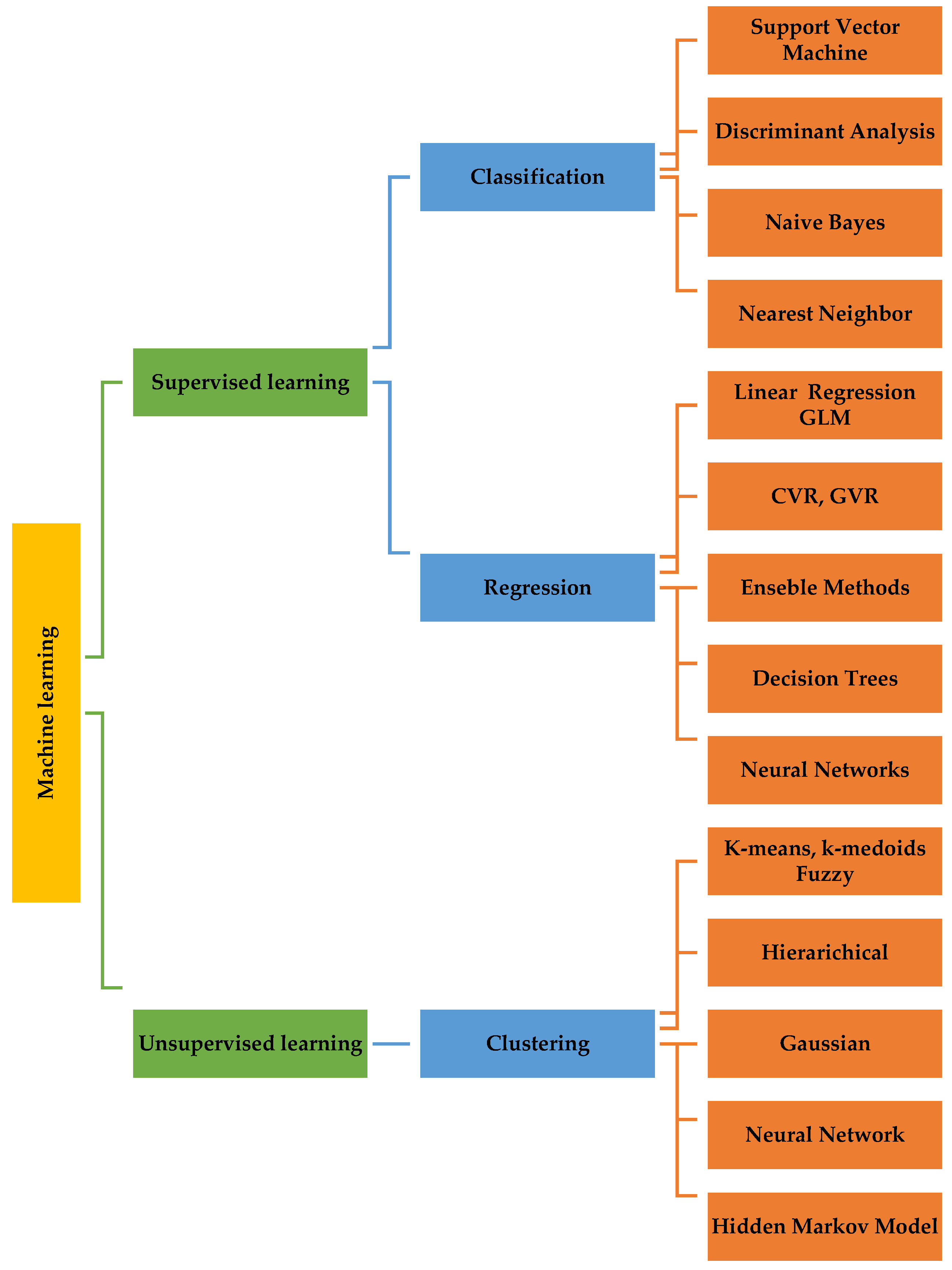
Deep Learning (DL) is a subsection of ML. In DL, a structure called ANN recognizes the perception of data. Neural networks are one set of algorithms used in ML for modeling the data [34,35,36]. A DL algorithm in the oil and gas industry improves the management of huge amounts of data and attains the best performance with large data [37]. Characters are extracted without human interference. DL algorithms perform complicated operations, while ML algorithms cannot. Inputs are run through neural networks. ANN is an effective ML technique for solving complex problems [38,39,40]. In oil and gas industries, ANN is mostly applied in nonlinear and complex problems which a linear relationship cannot solve.
Figure 1 shows the correlation among the expanded AI, ML, and DL fields.
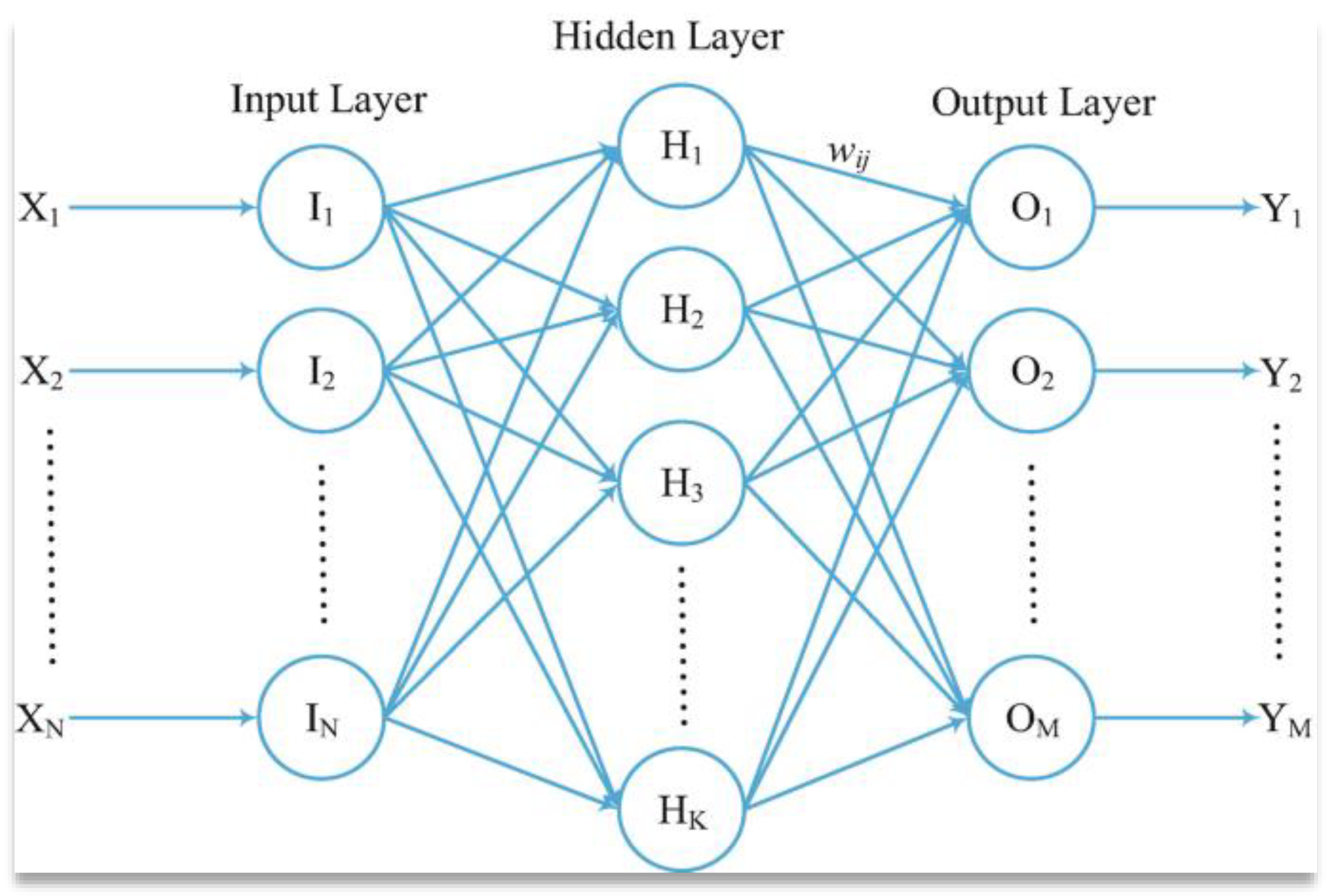
The ANN model helps to forecast pipeline conditions; it supports operators in evaluating and predicting the conditions of pipelines. The ML model can be employed to find the percentage of sand in the reservoir [41,42]. Figure 2 shows the basic structure of ANN.
ANN is knowledge based on brain and nervous system analyses, as depicted in Figure 2. These networks contend with a biological neural network, but they employ a lesser set of theories than biological neural systems. Mainly, ANN models simulate the brain and nervous system’s electrical activity [43,44]. Processing elements (also known as either a neuron or perceptron) are linked to other processing elements. Usually, the neurons are arranged in a layer or vector, with the output of one layer acting as the input to the next layer and possibly other layers [45,46]. A neuron may be linked to all or a subset of the neurons in the subsequent layer, with these connections simulating the brain’s synaptic networks. Weighted data signals entering a neuron simulate the electrical excitation of a nerve cell and, subsequently, the transmission of information within the network or brain [47,48].
The steps involved in ML are given in Figure 3.
The path forward keeps leveraging AI and ML-based skills, developing quickly and being implemented across the value chain. Numerous industries have revealed the advantages of this developing knowledge; consequently, we will continue to see more AI applications established in the future. In the framework of big data and manufacturing, ML techniques can manage high nonlinearity in complicated engineering predictions, consisting of energy, ecological science, hydrology, and construction [48].
An example of a complex neural network flowchart is shown in Figure 4.

3. Evaluation Methods

The overall condition index and neural network are presented in this part.

3.1. Overall Condition Index

To combine the effects of corrosion monitoring and cathodic protection parameters, it is necessary to normalize all monitored data. Equation (1), the Gaussian expression, performs this transformation [49].
C = e x r s 2
In this formula, C is the measurement of the normalization parameter, x is the value of the observed parameter, and r and s are the values calculated using Equations (2) and (3).
r = H + L 2
s = H L 2
H and L are each parameter’s upper and lower ranges, respectively. When x is equal to the value of its upper limit (H) or its lower limit (L), Equation (1) will become Equation (4).
C = e x r s 2 = e H L 2 2 H L 2 2 = e 1
C R indicates normalized constraints. This value can be used as a criterion for measuring the condition of the equipment in normal mode.
The equipment status is outside the defined range if the normalized parameter exceeds the C R value. If all the monitored C i parameters are shown after normalization, the overall condition index of corrosion will be in Equation (5).
Q = j = 1 N W i C i ,                                                                         A l l   C i > C R j = 1 M W i C i ,   A t   l e a s t   o n e   p a r a m e t e r   C i < C R
where N is the total number of normalized parameters, M is the total number of normalized parameters less than the value of C R and W i is the weighting coefficients of the importance of each parameter. Accordingly, the value of N is constant while the value of M will differ from the operating conditions of the equipment corrosion. W i values are selected to meet the following conditions:
i = 1 N W i = 1               o r               i = 1 M W i = 1  
No reference has examined which parameter is more important than the others. Accordingly, it is assumed that all the observed parameters are equally important [50].

3.2. Neural Network

According to the type of work, available data, and review of different neural networks, our selected network in this study is the nonlinear autoregressive with external input (NARX) dynamic neural network. The NARX structure is more accurate in estimation than other existing models. We want to evaluate the useful life of the three gas networks under CP and estimate the remaining useful life of the pipes. For this purpose, we can solve this problem by using the dynamic neural network and according to our data, which are continuous-time data, with the time series tool.
This network has a hidden layer, and the neurons number in this layer is considered trial and error of 10 neurons. The number of previous signals used in the model for the best fit is four for inputs and five for output. The stimulus function for latent layer neurons, the sigmoid function, and the output layer stimulus function are considered nonlinear.
To train the neural network, 70% of the data sampled by individuals and experts of the gas department has been applied. In addition, validation and test data sets are 15% of the original data. Using this data and the neural network toolbox in MATLAB, the neural network is trained and the nonlinear function f (nonlinear function of system inputs and outputs) is defined and it is determined that the output is shown after training.
The determination of indicators and their impact using sources, documents, and expert opinions is carried out according to approved standards (B31G (ANSI/ASME B31G) and B31.8 (ANSI/ASME B31.8)). Operating life is calculated by multiplying the calendar life by the effect of each effective indicator on the life of the relevant equipment and the coefficients related to the network conditions. Equation (7) shows this.
t f = i = 1 n W i T
This function is the functional age of the equipment, T is the actual life, W is the impact of the i th index, and i is the number of indicators affecting the operating life of the equipment.
The remaining operating life for each piece of equipment according to the multiplication of “standard remaining life” in the impact of each of the indicators affecting the life for the conditions in which the equipment is to operate in the future will be counted according to Equation (8).
R t f = i = 1 n 1 W i × t R
In this regard, R t f   is the operating life, and t R   is the standard life. The operating and standard life differences produce the remaining standard life from the following equation.
t R = t s t f
In this respect, t s is the standard life.

4. Data Monitoring

The data monitored in this paper were from 2013 to 2015.
  • The cathodic protection station (CPS) is set every 15 days, including pre-set voltage, pre-set current, pre-set injection voltage, pre-set cut-off voltage, post-set transformer voltage, and present, and the color is silica gel;
  • Test point measurement (TP) is carried out every four months. If it is in the form of a pool, the cleaning of the pool should also be carried out, and if it is in the form of science, it is measured from the three parts of the science valve, the sheath, and the surge arrester;
  • Measurement of flange insulation of turner broadcasting system (TBS) stations once every six months;
  • Anodic control is performed every six months to measure the flow of anodes;
  • Test the cover with a holiday device or by installing a current source by insulating the damaged points;
  • AC line voltage measurement (caused by stray currents), according to US NACL standards, can be omitted if it is less than 15 volts (every four months). This voltage enters the line from one point, and from where it exits it will cause corrosion of the pipe in the same place;
  • Existence of a protected structure next to a protected gas pipe (such as a water pipe). Additionally, two lines must be potentialized to prevent corrosion;
  • The presence of DC voltage (700 volts) on city trains is harmful;
  • The presence of AC voltage (20 kV) in the subway is harmful.
Therefore, according to the above, the data required for fault analysis are:
  • DC voltage of measuring points in gas networks; the normal value of this voltage is between 0.85 and 2.1 volts;
  • AC voltage of measuring points in gas networks; the maximum acceptable voltage is 15 volts;
  • DC voltage measuring points. Before adjusting, if the voltage value is more than 2.1 volts and less than 0.85 volts it should be checked;
  • The voltage of measuring points in the transformer off mode depends on the type of cover and transformer capacity;
  • Circuit resistance in GPS stations; if it is more than 3 ohms, the circuit should be checked;
  • Transformer output voltage depends on the injection voltage, and its value is adjusted according to the injection voltage;
  • Transformer output current is determined according to the surface of the pipe and the amount of damage to the cover;
  • Output current in 75 volts and 25 amps transformers can be from 1 to 25 amps;
  • Anode current rate: MMO in water is 8 amps, and silicon in water is 4 amps;
  • Water column: at the beginning of drilling, the well should be about 10 m above the anodes;
  • Circuit resistance: factors that increase it are lowering the water level, cable cross-section, end of anodes, incomplete coding, and sulfation of cable washer and busbars inbox.

5. Case Study

In this section, the results of the case study will be analyzed. As mentioned, two general methods of the general condition monitoring index and neural network method will be examined in this section.

5.1. Results from the Overall Condition Index

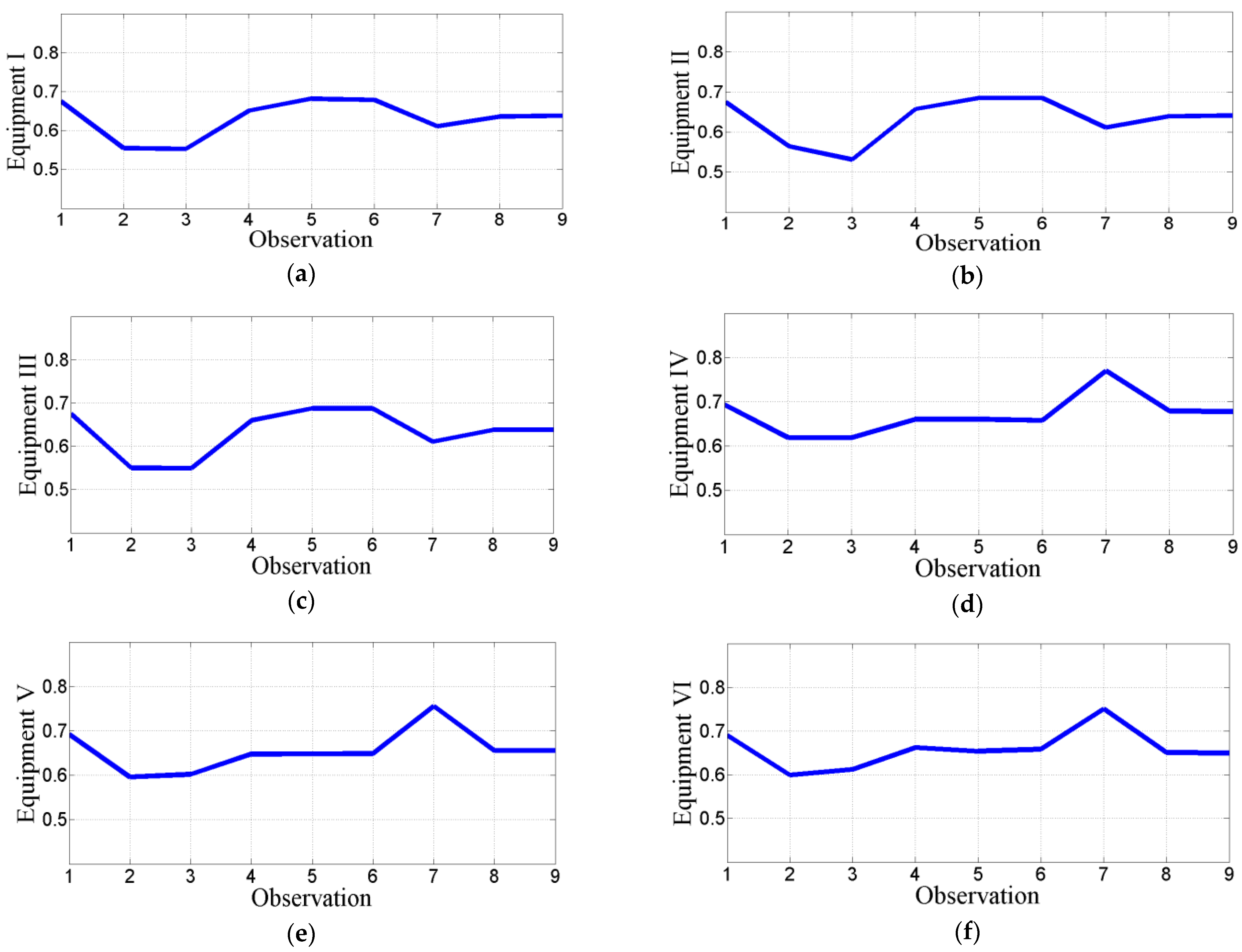
In the following, the conditions resulting from the general condition of the equipment will be checked. As can be seen in Figure 5, the overall condition index of the six types of equipment over time is examined. According to this analysis, the general equipment monitoring index trend is almost deteriorating. This procedure is unique for different equipment. In all the equipment, the index trend initially showed an improvement in the second sample and then went to failure. In equipment items 4, 5 and 6, the seventh data sample has the worst condition, while equipment items 1, 2 and 3 in these data have a much better situation. According to what has been said, when the values of these graphs are less than the value of e−1 = 0.367 the equipment conditions will be critical.
As a result of the complex state of the pipeline, the diagnostic approach based on the hypothetical model has weak reliability. To enhance this deficiency, ANN is applied to perform pattern recognition on the checking report. Leakage diagnosis is accomplished by evaluating the correlation between self-trained leakage points and symptoms of a neural network [51,52,53,54]. The leakage diagnosis method based on neural networks can prevent the computation and modeling of the pipeline network fluid parameters. Linear regression, ANN, and SVM are the ML methods normally employed. Compared with linear regression, ANN and SVM offer greater prediction accuracy. Recent research papers described how improved optimization algorithms could improve ML training. The improvement of the hybrid models develops prediction accuracy, which has been extensively applied in pipeline activities, including failure pressure prediction, leakage checking and reliability assessment. It is suggested that ML techniques can be applied to train the simulations with complicated physical structures [55,56,57,58]. Figure 6 also shows the monitoring of equipment conditions. According to this figure, the difference in equipment conditions is quite apparent.

5.2. Predicting the Failure Time of Cathodic Protection by the Neural Network

For this case study, we selected the NARX model of the neural network and used the Levenberg–Marquardt train model. A multilayer perceptron neural network estimated the remaining useful life. After performing the simulation with MATLAB software, we examined the output details. Figure 7 can predict the failure time of CP. The blue line is the training results, the green line is the validation result, and the red line is the test data. Due to the lack of data in this diagram, the training data diagram (train data) fits poorly with the test data diagram. Validation of the network training accuracy is possible by matching proof and test charts. When the training data diagram is most different from the test data, and there are sudden changes in the test data diagram, it is time to pay more attention to the CP system and check the condition of the tube.
Most preceding leakage diagnosis approaches were based on static rules; the technique requires controlling all the information of the gas flow principle and microscopic model of the pipeline. The checking value of the same node was influenced by the position of various leakage points [59,60,61]. Moreover, uncertain aspects including medium composition and working conditions made it complicated to establish the constraints needed for modeling, which made it easy to cause errors or mistake diagnoses. The operating conditions of the extraction pipeline were time-consuming and complicated, so the traditional leakage diagnosis method of the pipeline cannot reflect the leakage state of the pipeline [62,63,64,65]. To solve the problem of precisely diagnosing and locating leakage points in gas extraction pipelines, a method combining laboratory experiments and ML is proposed in this study. The suggested approach considered the power of various input parameters on diagnostic and positioning accuracy. According to Figure 8, when the CP is used correctly, the data scatter will be less than the regression line.
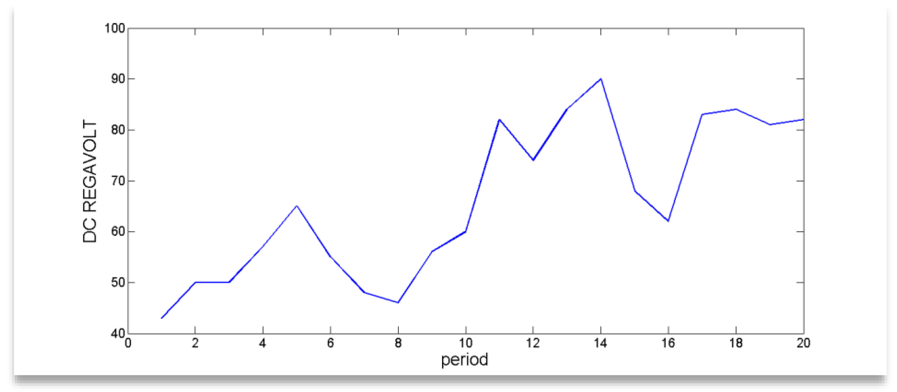
Figure 9 shows the Regavolt for 20 periods related to the Nazarabad city pipeline. The period is three months, and the amount of Regavolt is in terms of distance. Regavolt changes from zero to one hundred and fifty. If the amount of Regavolt is more than one hundred, the short visit period and the network should be monitored, and the necessary checks should be made on the pipe.
Data are available for up to twenty periods. Over time and by recording more data, it will be possible to draw a graph based on Figure 10. In this study, 120 periods are given for the sample, which can be drawn from the beginning to the end until the tube is replaced. Additionally, Regavolt is the line voltage regulator; therefore, changes in it must be considered.
Potential differences are measured and recorded at stations before and after transformers based on Figure 11. If this difference is significant, the visit periods will be shortened and the network will be monitored.
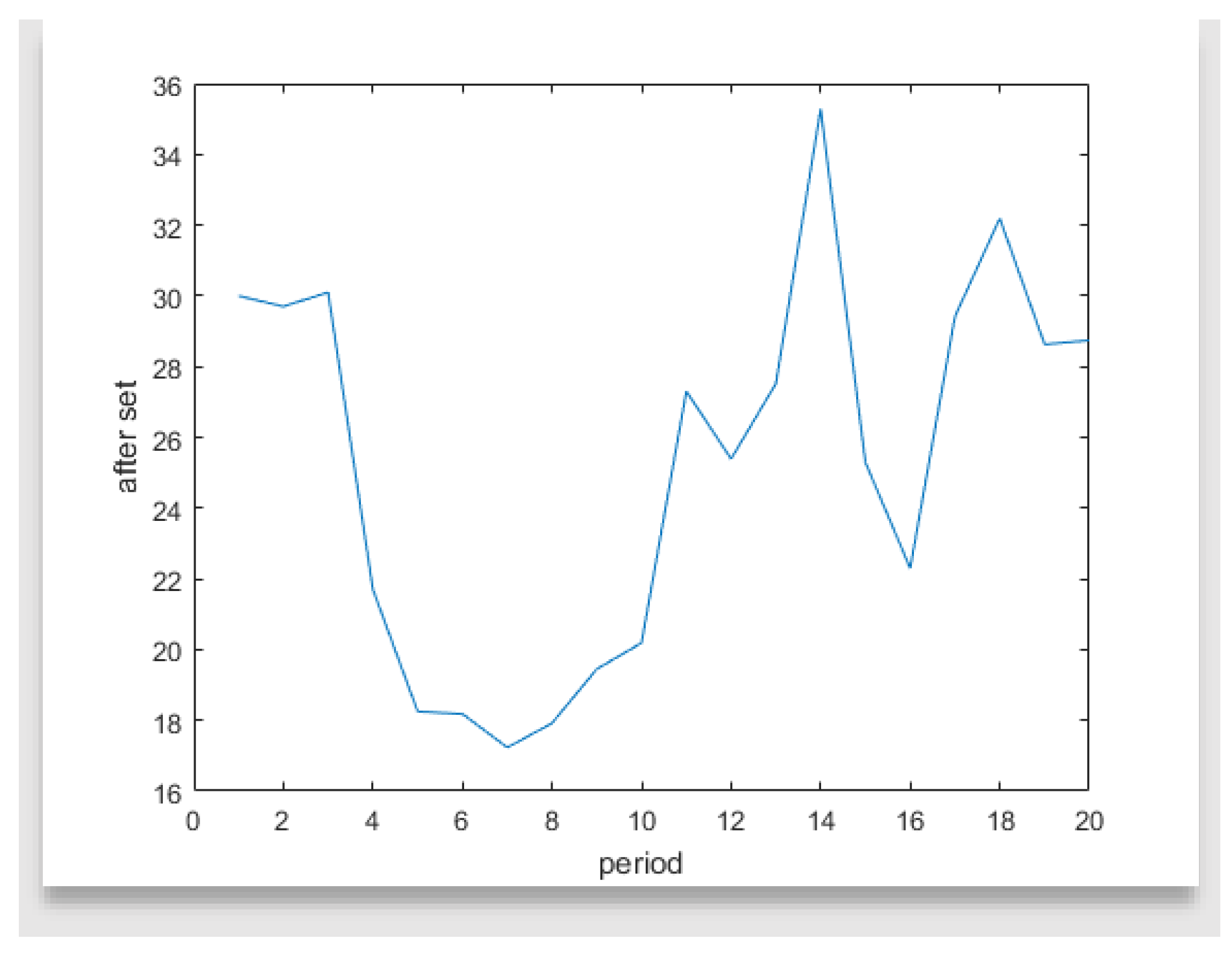
The potential difference is measured after adjustment based on Figure 12. If this value is more than 0.5 volts, the short visit period and the network should be monitored.
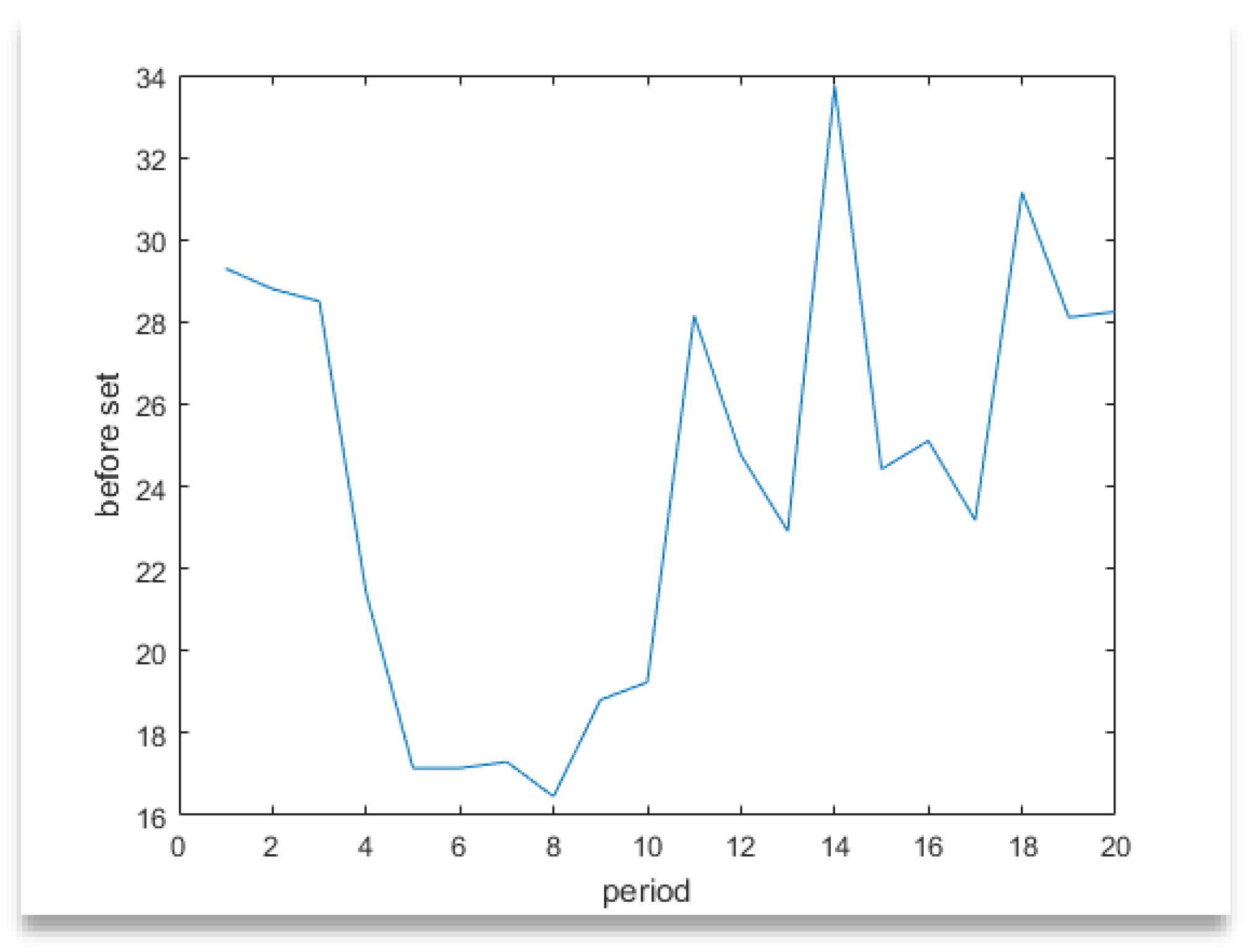
The potential difference is measured before adjustment based on Figure 13. If the potential difference value is more than 0.5 volts, the short visit period and the network should be monitored.
The comparison of implementing this method with the previous methods is described in Table 1. It is worth noting that the results of the two ways are close to each other. As a result, the correctness of the implementation steps of the new method is confirmed.
The previous model calculates the remaining life using standard organizational, operating and calendar life. The basis of the calculations is the application of indicators determined in mathematical formulas [66,67,68,69], while in the new method neural networks with more accuracy in estimation are used. Scientists have preferred ANN-based-predictive models in this domain against other AI methods because of the following advantages [70,71,72,73,74]:
  • Consistent prediction, and compatibility with other building energy simulation software [75,76,77];
  • Overcoming the nonlinearity among the energy-related data inputs and outputs [78,79];
  • Since training in applying ANN is not as expensive as traditional data collection (such as theoretical-based or empirical-based techniques), progressively more scientists are becoming attracted to the development of ANN [80,81].
One interesting thing about ANN is that they are trained, instead of being designed to perform specific tasks concerning data sets until they learn the patterns given to them [82,83,84,85].

6. Conclusions

In this paper, the effect of stray currents on estimating the remaining useful life of gas pipes under CP was investigated using an overall condition index of equipment and neural networks. According to the comprehensive condition index, the general equipment monitoring index trend was almost deteriorating, which was seen differently for different equipment. In all the types of equipment, the index trend initially improved in the second sample and then declined. Next, we proposed a model of neural networks. A multilayer perceptron neural network was used to estimate the remaining useful life. After studying and evaluating different optimization methods and selecting the appropriate method, MATLAB was used to assess and measure it and prove its optimality after simulation. In addition to estimating the remaining useful life of equipment in the industry, it manages the commercial risks that result from malfunctions and failures in the operation of devices. Industry, economic aspects, maintaining production safety, weighing preventing life and financial loss, applying high-reliability coefficients, analyzing unwanted stresses, unforeseen environmental and operational factors, applying outside design ranges (such as high temperature and cyclic load), the reduction of material properties in service in sensitive areas, experience, and damage analysis are factors identified in the case study. In addition to stating the extent of the failure and the remaining useful life, this article plans and announces the next visit time according to the pipe conditions and the latest information. Supposing that the existing equipment conditions in the current repair plan of the gas company are fine with future planning, this plan can be an excellent alternative to the existing repair plan.

Future Study

According to the proposed procedure, by updating the data obtained from any equipment in the future its life and failure rate can be estimated. Based on this, new data can be given to the neural network and its training can be made more complete, or the rate of failure in each period can be estimated. In addition, based on the evaluations in this study, CP is one of the most important contributors to pipeline condition prediction. However, other factors including metal loss, coating condition, age, support condition, joint condition, anode wastage, and free spans are still important for pipeline condition prediction and should be considered for future studies. Finally, the majority of the improved condition evaluation models are either subjective (i.e., dependent only on expert opinions, considering no historical data), or incomplete (i.e., considering just one failure cause). The objective of future research should be to develop a more comprehensive condition evaluation model that allows pipeline operators to take the required activities to avoid future devastating failures.

Author Contributions

Methodology, H.N., M.G., J.N., A.A. and M.M.; Conceptualization, H.N., M.G. and M.M.; Software, J.N., A.A. and M.G.; Validation, H.N.; Formal Analysis, M.G. and M.M.; Investigation, M.M.; Resources, H.N., A.A. and M.M.; Data Curation, H.N., M.G. and M.M.; Writing—Original Draft Preparation, M.M.; Writing—Review and Editing, M.M.; Visualization, J.N., A.A. and M.M.; Supervision, M.M.; Project Administration, H.N., M.G., J.N. and A.A. All authors have read and agreed to the published version of the manuscript.

Funding

This research received no external funding.

Data Availability Statement

The data used in the study are available from the authors and can be accessed upon acceptable request.

Acknowledgments

The authors would like to thank the reviewers and the editor-in-chief for their helpful comments and recommendations.

Conflicts of Interest

The authors declare no conflict of interest.

References

  1. Zhang, X.; Xiao, P.; Yang, Y.; Cheng, Y.; Chen, B.; Gao, D.; Liu, W.; Huang, Z. Remaining useful life estimation using CNN-XGB with extended time window. IEEE Access 2019, 7, 154386–154397. [Google Scholar] [CrossRef]
  2. Das, A.; Hussain, S.; Yang, F.; Habibullah, M.S.; Kumar, A. Deep recurrent architecture with attention for remaining useful life estimation. In Proceedings of the TENCON 2019–2019 IEEE Region 10 Conference (TENCON), Kochi, India, 17–20 October 2019; pp. 2093–2098. [Google Scholar]
  3. Zhang, J.; Wang, S.; Chen, L.; Guo, G.; Chen, R.; Vanasse, A. Time-dependent survival neural network for remaining useful life prediction. In Proceedings of the Pacific-Asia Conference on Knowledge Discovery and Data Mining, Macau, China, 14–17 April 2019; Springer: Cham, Switzerland; pp. 441–452. [Google Scholar]
  4. Kordestani, M.; Samadi, M.F.; Saif, M. A new hybrid fault prognosis method for MFS systems based on distributed neural networks and recursive bayesian algorithm. IEEE Syst. J. 2020, 14, 5407–5416. [Google Scholar] [CrossRef]
  5. Mezzi, R.; Morando, S.; Steiner, N.Y.; Péra, M.C.; Hissel, D.; Larger, L. Multi-reservoir echo state network for proton exchange membrane fuel cell remaining useful life prediction. In Proceedings of the IECON 2018-44th Annual Conference of the IEEE Industrial Electronics Society, Washington, DC, USA, 21–23 October 2018; pp. 1872–1877. [Google Scholar]
  6. Polder, R.B.; Leegwater, G.; Worm, D.; Courage, W. Service life and life cycle cost modelling of cathodic protection systems for concrete structures. Cem. Concr. Compos. 2014, 47, 69–74. [Google Scholar] [CrossRef] [Green Version]
  7. Tang, K. Stray alternating current (AC) induced corrosion of steel fibre reinforced concrete. Corros. Sci. 2019, 152, 153–171. [Google Scholar] [CrossRef] [Green Version]
  8. Wang, Y.; Li, Z.; He, H.; Lu, W.; Xu, Y.; Mao, Y. An Inductance Forcedly Absorbing Current Circuit to Reduce the Stray Current in the DC Power Supply System. In Proceedings of the 2019 14th IEEE Conference on Industrial Electronics and Applications (ICIEA), Xi’an, China, 19–21 June 2019; pp. 2303–2308. [Google Scholar]
  9. Avdeeva, K.V. Experimental Research of Stray Currents Influence of DC Railway Transport to Grounding Grid. In Proceedings of the 2019 Dynamics of Systems, Mechanisms and Machines (Dynamics), Omsk, Russia, 5–7 November 2019; pp. 1–4. [Google Scholar]
  10. Zhao, L.P.; Li, J.H.; Liu, M.J. Simulation and analysis of metro stray current based on multi-locomotives condition. In Proceedings of the 2016 35th Chinese Control Conference (CCC), Chengdu, China, 27–29 July 2016; pp. 9252–9258. [Google Scholar]
  11. Liu, W.; Li, T.; Zheng, J.; Pan, W.; Yin, Y. Evaluation of the Effect of Stray Current Collection System in DC-Electrified Railway System. IEEE Trans. Veh. Technol. 2021, 70, 6542–6553. [Google Scholar] [CrossRef]
  12. Yuan, P.; Mao, W.; Ye, H.; Liu, Y. Model Construction and Analysis of Transformer DC Magnetic Bias Induced by Rail Transit Stray Current. In Proceedings of the 2019 IEEE 3rd Conference on Energy Internet and Energy System Integration (EI2), Changsha, China, 8–10 November 2019; pp. 1710–1713. [Google Scholar]
  13. Lin, Y.; Li, K.; Su, M.; Meng, Y. Research on stray current distribution of metro based on numerical simulation. In Proceedings of the 2018 IEEE International Symposium on Electromagnetic Compatibility and 2018 IEEE Asia-Pacific Symposium on Electromagnetic Compatibility (EMC/APEMC), Suntec City, Singapore, 14–18 May 2018; pp. 36–40. [Google Scholar]
  14. Mirmozaffari, M.; Yazdani, R.; Shadkam, E.; Khalili, S.M.; Mahjoob, M.; Boskabadi, A. An integrated artificial intelligence model for efficiency assessment in pharmaceutical companies during the COVID-19 pandemic. Sustain. Oper. Comput. 2022, 3, 156–167. [Google Scholar] [CrossRef]
  15. Mirmozaffari, M.; Shadkam, E.; Khalili, S.M.; Yazdani, M. Developing a novel integrated generalised data envelopment analysis (DEA) to evaluate hospitals providing stroke care services. Bioengineering 2021, 8, 207. [Google Scholar] [CrossRef]
  16. El-Abbasy, M.S.; Senouci, A.; Zayed, T.; Mirahadi, F.; Parvizsedghy, L. Artificial neural network models for predicting condition of offshore oil and gas pipelines. Autom. Constr. 2014, 45, 50–65. [Google Scholar] [CrossRef]
  17. Mirmozaffari, M.; Yazdani, R.; Shadkam, E.; Tavassoli, L.S.; Massah, R. VCS and CVS: New combined parametric and non-parametric operation research models. Sustain. Oper. Comput. 2021, 2, 36–56. [Google Scholar] [CrossRef]
  18. Mirmozaffari, M.; Shadkam, E.; Khalili, S.M.; Kabirifar, K.; Yazdani, R.; Gashteroodkhani, T.A. A novel artificial intelligent approach: Comparison of machine learning tools and algorithms based on optimization DEA Malmquist productivity index for eco-efficiency evaluation. Int. J. Energy Sect. Manag. 2021, 15, 523–550. [Google Scholar] [CrossRef]
  19. Yazdani, M.; Jolai, F. Lion optimization algorithm (LOA): A nature-inspired metaheuristic algorithm. J. Comput. Des. Eng. 2016, 3, 24–36. [Google Scholar] [CrossRef] [Green Version]
  20. Zheng, J.; Liang, Y.; Xu, N.; Wang, B.; Zheng, T.; Li, Z.; Liao, Q.; Zhang, H. Deeppipe: A customized generative model for estimations of liquid pipeline leakage parameters. Comput. Chem. Eng. 2021, 149, 107290. [Google Scholar] [CrossRef]
  21. Al-Waeli, A.H.; Sopian, K.; Kazem, H.A.; Yousif, J.H.; Chaichan, M.T.; Ibrahim, A.; Mat, S.; Ruslan, M.H. Comparison of prediction methods of PV/T nanofluid and nano-PCM system using a measured dataset and artificial neural network. Sol. Energy 2018, 162, 378–396. [Google Scholar] [CrossRef]
  22. Aranizadeh, A.; Niazazari, I.; Mirmozaffari, M. A novel optimal distributed generation planning in distribution network using cuckoo optimization algorithm. Eur. J. Electr. Eng. Comput. Sci. 2019, 3. [Google Scholar] [CrossRef] [Green Version]
  23. Aranizadeh, A.; Kazemi, M.; Barahmandpour, H.; Mirmozaffari, M. MULTIMOORA Decision Making Algorithm for Expansion of HVDC and EHVAC in Developing Countries (A Case Study). Iran. J. Optim. 2020, 12, 63–71. [Google Scholar]
  24. Yazdani, R.; Mirmozaffari, M.; Shadkam, E.; Khalili, S.M. A Lion Optimization Algorithm for a Two-Agent Single-Machine Scheduling with Periodic Maintenance to Minimize the Sum of Maximum Earliness and Tardiness. Int. J. Ind. Syst. Eng. 2022. [Google Scholar] [CrossRef]
  25. Mirmozaffari, M.; Yazdani, M.; Boskabadi, A.; Ahady Dolatsara, H.; Kabirifar, K.; Amiri Golilarz, N. A novel machine learning approach combined with optimization models for eco-efficiency evaluation. Appl. Sci. 2020, 10, 5210. [Google Scholar] [CrossRef]
  26. Seghier, M.E.; Keshtegar, B.; Taleb-Berrouane, M.; Abbassi, R.; Trung, N.T. Advanced intelligence frameworks for predicting maximum pitting corrosion depth in oil and gas pipelines. Process Saf. Environ. Prot. 2021, 147, 818–833. [Google Scholar] [CrossRef]
  27. Shadkam, E.; Yazdani, R.; Mirmozaffari, M.; Adineh, F. The Hybrid DHP Method for Evaluation, Ranking, and Selection of Green Suppliers in the Supply Chain. Int. J. Math. Oper. Res. 2022. [Google Scholar] [CrossRef]
  28. Dawood, T.; Elwakil, E.; Novoa, H.M.; Delgado, J.F. Artificial intelligence for the modeling of water pipes deterioration mechanisms. Autom. Constr. 2020, 120, 103398. [Google Scholar] [CrossRef]
  29. Hu, X.; Zhang, H.; Ma, D.; Wang, R. A tnGAN-based leak detection method for pipeline network considering incomplete sensor data. IEEE Trans. Instrum. Meas. 2020, 70, 3510610. [Google Scholar] [CrossRef]
  30. Mirmozaffari, M.; Yazdani, R.; Shadkam, E.; Khalili, S.M.; Tavassoli, L.S.; Boskabadi, A. A novel hybrid parametric and non-parametric optimisation model for average technical efficiency assessment in public hospitals during and post-COVID-19 pandemic. Bioengineering 2021, 9, 7. [Google Scholar] [CrossRef] [PubMed]
  31. Sony, S.; Dunphy, K.; Sadhu, A.; Capretz, M. A systematic review of convolutional neural network-based structural condition assessment techniques. Eng. Struct. 2021, 226, 111347. [Google Scholar] [CrossRef]
  32. Tran, D.H.; Ng, A.W.; Perera, B.J.; Burn, S.; Davis, P. Application of probabilistic neural networks in modelling structural deterioration of stormwater pipes. Urban Water J. 2006, 3, 175–184. [Google Scholar] [CrossRef] [Green Version]
  33. Rahimi, A.; Hejazi, S.M.; Zandieh, M.; Mirmozaffari, M. A Novel Hybrid Simulated Annealing for No-Wait Open-Shop Surgical Case Scheduling Problems. Appl. Syst. Innov. 2023, 6, 15. [Google Scholar] [CrossRef]
  34. Parashar, A.; Parashar, A.; Ding, W.; Shekhawat, R.S.; Rida, I. Deep learning pipelines for recognition of gait biometrics with covariates: A comprehensive review. Artif. Intell. Rev. 2023, 1–65. [Google Scholar] [CrossRef]
  35. Chaki, S.; Routray, A.; Mohanty, W.K. Well-log and seismic data integration for reservoir characterization: A signal processing and machine-learning perspective. IEEE Signal Process. Mag. 2018, 35, 72–81. [Google Scholar] [CrossRef]
  36. Ahmad, Z.; Nguyen, T.K.; Kim, J.M. Leak detection and size identification in fluid pipelines using a novel vulnerability index and 1-D convolutional neural network. Eng. Appl. Comput. Fluid Mech. 2023, 17, 2165159. [Google Scholar] [CrossRef]
  37. Yazdani, M.; Kabirifar, K.; Frimpong, B.E.; Shariati, M.; Mirmozaffari, M.; Boskabadi, A. Improving construction and demolition waste collection service in an urban area using a simheuristic approach: A case study in Sydney, Australia. J. Clean. Prod. 2021, 280, 124138. [Google Scholar] [CrossRef]
  38. Yazdani, R.; Mirmozaffari, M.; Shadkam, E.; Taleghani, M. Minimizing total absolute deviation of job completion times on a single machine with maintenance activities using a Lion Optimization Algorithm. Sustain. Oper. Comput. 2022, 3, 10–16. [Google Scholar] [CrossRef]
  39. Bayat, R.; Talatahari, S.; Gandomi, A.H.; Habibi, M.; Aminnejad, B. Artificial Neural Networks for Flexible Pavement. Information 2023, 14, 62. [Google Scholar] [CrossRef]
  40. Sandhu, H.K.; Bodda, S.S.; Gupta, A. Post-hazard condition assessment of nuclear piping-equipment systems: Novel approach to feature extraction and deep learning. Int. J. Press. Vessel. Pip. 2023, 201, 104849. [Google Scholar] [CrossRef]
  41. Yesilnacar, E.; Topal, T.A. Landslide susceptibility mapping: A comparison of logistic regression and neural networks methods in a medium scale study, Hendek region (Turkey). Eng. Geol. 2005, 79, 251–266. [Google Scholar] [CrossRef]
  42. Atambo, D.O.; Najafi, M.; Kaushal, V. Development and Comparison of Prediction Models for Sanitary Sewer Pipes Condition Assessment Using Multinomial Logistic Regression and Artificial Neural Network. Sustainability 2022, 14, 5549. [Google Scholar] [CrossRef]
  43. Yang, Y.; Li, S.; Zhang, P. Data-driven accident consequence assessment on urban gas pipeline network based on machine learning. Reliab. Eng. Syst. Saf. 2022, 219, 108216. [Google Scholar] [CrossRef]
  44. Pal, R.; Sekh, A.A.; Kar, S.; Prasad, D.K. Neural network based country wise risk prediction of COVID-19. Appl. Sci. 2020, 10, 6448. [Google Scholar] [CrossRef]
  45. Mirmozaffari, M. Filtering in Image Processing. ENG Trans. 2020, 1, 1–5. [Google Scholar]
  46. Kumari, P.; Halim, S.Z.; Kwon, J.S.; Quddus, N. An integrated risk prediction model for corrosion-induced pipeline incidents using artificial neural network and Bayesian analysis. Process Saf. Environ. Prot. 2022, 167, 34–44. [Google Scholar] [CrossRef]
  47. Elshaboury, N.; Abdelkader, E.M.; Al-Sakkaf, A.; Alfalah, G. Teaching-learning-based optimization of neural networks for water supply pipe condition prediction. Water 2021, 13, 3546. [Google Scholar] [CrossRef]
  48. Roshani, M.; Phan, G.T.; Ali, P.J.; Roshani, G.H.; Hanus, R.; Duong, T.; Corniani, E.; Nazemi, E.; Kalmoun, E.M. Evaluation of flow pattern recognition and void fraction measurement in two phase flow independent of oil pipeline’s scale layer thickness. Alex. Eng. J. 2021, 60, 1955–1966. [Google Scholar] [CrossRef]
  49. Zhang, D.; Li, W.; Xiong, X.; Liao, R. Evaluating condition index and its probability distribution using monitored data of circuit breaker. Electr. Power Compon. Syst. 2011, 39, 965–978. [Google Scholar] [CrossRef]
  50. Zhong, J.; Li, W.; Billinton, R.; Yu, J. Incorporating a condition monitoring based aging failure model of a circuit breaker in substation reliability assessment. IEEE Trans. Power Syst. 2015, 30, 3407–3415. [Google Scholar] [CrossRef]
  51. Mirmozaffari, M. Eco-Efficiency Evaluation in Two-Stage Network Structure: Case Study: Cement Companies. Iran. J. Optim. 2019, 11, 125–135. [Google Scholar]
  52. Haseli, G.; Ranjbarzadeh, R.; Hajiaghaei-Keshteli, M.; Ghoushchi, S.J.; Hasani, A.; Deveci, M.; Ding, W. HECON: Weight assessment of the product loyalty criteria considering the customer decision’s halo effect using the convolutional neural networks. Inf. Sci. 2023, 623, 184–205. [Google Scholar] [CrossRef]
  53. Mirmozaffari, M. An Improved Non-dominated Sorting Method in Genetic Algorithm for Bi-objective Problems. ENG Trans. 2021, 2, 1–7. [Google Scholar]
  54. Calisir, T.; Çolak, A.B.; Aydin, D.; Dalkilic, A.S.; Baskaya, S. Artificial neural network approach for investigating the impact of convector design parameters on the heat transfer and total weight of panel radiators. Int. J. Therm. Sci. 2023, 183, 107845. [Google Scholar] [CrossRef]
  55. Wang, B.W.; Tang, W.Z.; Song, L.K.; Bai, G.C. Deep neural network-based multiagent synergism method of probabilistic HCF evaluation for aircraft compressor rotor. Int. J. Fatigue 2023, 170, 107510. [Google Scholar] [CrossRef]
  56. Niu, S.; Zhang, E.; Bazilevs, Y.; Srivastava, V. Modeling finite-strain plasticity using physics-informed neural network and assessment of the network performance. J. Mech. Phys. Solids 2023, 172, 105177. [Google Scholar] [CrossRef]
  57. Diao, Y.; Jelescu, I. Parameter estimation for WMTI-Watson model of white matter using encoder–decoder recurrent neural network. Magn. Reson. Med. 2023, 89, 1193–1206. [Google Scholar] [CrossRef]
  58. Miao, X.; Zhao, H.; Xiang, Z. Leakage detection in natural gas pipeline based on unsupervised learning and stress perception. Process Saf. Environ. Prot. 2023, 170, 76–88. [Google Scholar] [CrossRef]
  59. Zou, Z.; Ergan, S. Towards emotionally intelligent buildings: A Convolutional neural network based approach to classify human emotional experience in virtual built environments. Adv. Eng. Inform. 2023, 55, 101868. [Google Scholar] [CrossRef]
  60. Tajjour, S.; Garg, S.; Chandel, S.S.; Sharma, D. A novel hybrid artificial neural network technique for the early skin cancer diagnosis using color space conversions of original images. Int. J. Imaging Syst. Technol. 2023, 33, 276–286. [Google Scholar] [CrossRef]
  61. Wang, K.; Xu, C.; Li, G.; Zhang, Y.; Zheng, Y.; Sun, C. Combining convolutional neural networks and self-attention for fundus diseases identification. Sci. Rep. 2023, 13, 76. [Google Scholar] [CrossRef] [PubMed]
  62. Rasheed, H.A.; Davis, T.; Morales, E.; Fei, Z.; Grassi, L.; De Gainza, A.; Nouri-Mahdavi, K.; Caprioli, J. RimNet: A Deep Neural Network Pipeline for Automated Identification of the Optic Disc Rim. Ophthalmol. Sci. 2023, 3, 100244. [Google Scholar] [CrossRef]
  63. Amiri, M.H. Uncertainty Quantification in Neural Network-Based Classification Models. Ph.D. Thesis, University of Ottawa, Ottawa, ON, Canada, 2023. [Google Scholar]
  64. Oei, R.W.; Hsu, W.; Lee, M.L.; Tan, N.C. Using similar patients to predict complication in patients with diabetes, hypertension, and lipid disorder: A domain knowledge-infused convolutional neural network approach. J. Am. Med. Inform. Assoc. 2023, 30, 273–281. [Google Scholar] [CrossRef]
  65. Nogay, H.S.; Adeli, H. Diagnostic of autism spectrum disorder based on structural brain MRI images using, grid search optimization, and convolutional neural networks. Biomed. Signal Process. Control 2023, 79, 104234. [Google Scholar] [CrossRef]
  66. Rong, K.; Fu, M.; Huang, Y.; Zhang, M.; Zheng, L.; Zheng, J.; Scholz, M.; Yaseen, Z.M. Graph attention neural network for water network partitioning. Appl. Water Sci. 2023, 13, 1–14. [Google Scholar] [CrossRef]
  67. Yang, D.; Zhang, X.; Zhou, T.; Wang, T.; Li, J. A Novel Pipeline Corrosion Monitoring Method Based on Piezoelectric Active Sensing and CNN. Sensors 2023, 23, 855. [Google Scholar] [CrossRef]
  68. Pérez, E.; Ventura, S. A framework to build accurate Convolutional Neural Network models for melanoma diagnosis. Knowl.-Based Syst. 2023, 260, 110157. [Google Scholar] [CrossRef]
  69. Singh, P.B.; Singh, P.; Dev, H. Optimized convolutional neural network for glaucoma detection with improved optic-cup segmentation. Adv. Eng. Softw. 2023, 175, 103328. [Google Scholar] [CrossRef]
  70. Peykani, P.; Seyed Esmaeili, F.S.; Mirmozaffari, M.; Jabbarzadeh, A.; Khamechian, M. Input/output variables selection in data envelopment analysis: A shannon entropy approach. Mach. Learn. Knowl. Extr. 2022, 4, 688–699. [Google Scholar] [CrossRef]
  71. Mahjoob, M.; Fazeli, S.S.; Tavassoli, L.S.; Mirmozaffari, M.; Milanlouei, S. A green multi-period inventory routing problem with pickup and split delivery: A case study in flour industry. Sustain. Oper. Comput. 2021, 2, 64–70. [Google Scholar] [CrossRef]
  72. Mahjoob, M.; Fazeli, S.S.; Milanlouei, S.; Tavassoli, L.S.; Mirmozaffari, M. A modified adaptive genetic algorithm for multi-product multi-period inventory routing problem. Sustain. Oper. Comput. 2022, 3, 1–9. [Google Scholar] [CrossRef]
  73. Tavassoli, L.S.; Massah, R.; Montazeri, A.; Mirmozaffari, M.; Jiang, G.J.; Chen, H.X. A new multiobjective time-cost trade-off for scheduling maintenance problem in a series-parallel system. Math. Probl. Eng. 2021, 2021, 5583125. [Google Scholar] [CrossRef]
  74. Azeem, G.; Mirmozaffari, M.; Yazdani, R.; Khan, R.A. Exploring the impacts of COVID-19 pandemic on risks faced by infrastructure projects in Pakistan. Int. J. Appl. Decis. Sci. 2022, 15, 181–200. [Google Scholar] [CrossRef]
  75. Golilarz, N.A.; Mirmozaffari, M.; Gashteroodkhani, T.A.; Ali, L.; Dolatsara, H.A.; Boskabadi, A.; Yazdi, M. Optimized wavelet-based satellite image de-noising with multi-population differential evolution-assisted harris hawks optimization algorithm. IEEE Access 2020, 8, 133076–133085. [Google Scholar] [CrossRef]
  76. Mirmozaffari, M.; Alinezhad, A. Ranking of Heart Hospitals Using cross-efficiency and two-stage DEA. In Proceedings of the 2017 7th International Conference on Computer and Knowledge Engineering (ICCKE), Mashhad, Iran, 26–27 October 2017; pp. 217–222. [Google Scholar]
  77. Boskabadi, A.; Mirmozaffari, M.; Yazdani, R.; Farahani, A. Design of a distribution network in a multi-product, multi-period green supply chain system under demand uncertainty. Sustain. Oper. Comput. 2022, 3, 226–237. [Google Scholar] [CrossRef]
  78. Peykani, P.; Memar-Masjed, E.; Arabjazi, N.; Mirmozaffari, M. Dynamic performance assessment of hospitals by applying credibility-based fuzzy window data envelopment analysis. Healthcare 2022, 10, 876. [Google Scholar] [CrossRef]
  79. Mirmozaffari, M.; Zandieh, M.; Hejazi, S.M. An Output Oriented Window Analysis Using Two-stage DEA in Heart Hospitals. In Proceedings of the 10th International Conference on Innovations in Science, Engineering, Computers and Technology (ISECT-2017), Dubai, United Arab Emirates, 17–19 October 2017. [Google Scholar]
  80. Mirmozaffari, M.; Zandieh, M.; Hejazi, S.M. A Cloud Theory-based Simulated Annealing for Discovering Process Model from Event Logs. In Proceedings of the 10th International Conference on Innovations in Science, Engineering, Computers and Technology (ISECT-2017), Dubai, United Arab Emirates, 17–19 October 2017; Dignified Researchers Publication: Sahibzada Ajit Singh Nagar, India; pp. 70–75. [Google Scholar]
  81. Mirmozaffari, M.; Alinezhad, A. Window analysis using two-stage DEA in heart hospitals. In Proceedings of the 10th International Conference on Innovations in Science, Engineering, Computers and Technology (ISECT-2017), Dubai, United Arab Emirates, 17–19 October 2017; pp. 44–51. [Google Scholar]
  82. Mirmozaffari, M.; Golilarz, N.A.; Band, S.S. Machine Learning Algorithms Based on an Optimization Model. Preprints 2020, 2020090729. [Google Scholar] [CrossRef]
  83. Khan, A.; Rajendran, P.; Sidhu, J.S.; Thanigaiarasu, S.; Raja, V.; Al-Mdallal, Q. Convolutional neural network modeling and response surface analysis of compressible flow at sonic and supersonic Mach numbers. Alex. Eng. J. 2023, 65, 997–1029. [Google Scholar] [CrossRef]
  84. Wilberforce, T.; Alaswad, A.; Garcia–Perez, A.; Xu, Y.; Ma, X.; Panchev, C. Remaining useful life prediction for proton exchange membrane fuel cells using combined convolutional neural network and recurrent neural network. Int. J. Hydrogen Energy 2023, 48, 291–303. [Google Scholar] [CrossRef]
  85. Qi, J.; Yang, C.H.; Chen, P.Y.; Tejedor, J. Exploiting Low-Rank Tensor-Train Deep Neural Networks Based on Riemannian Gradient Descent with Illustrations of Speech Processing. IEEE/ACM Trans. Audio Speech Lang. Process. 2023, 31, 633–642. [Google Scholar] [CrossRef]
Figure 1. The correlation among the expanded AI, ML, and DL fields.
Make 05 00016 g001
Figure 2. The correlation among the expanded AI, ML and DL fields.
Make 05 00016 g002
Figure 3. Steps involved in ML problems.
Make 05 00016 g003
Figure 4. An example of a complex neural network flowchart.
Make 05 00016 g004
Figure 5. Monitoring the general condition of equipment, (a) Equipment item 1, (b) Equipment item 2, (c) Equipment item 3, (d) Equipment item 4, (e) Equipment item 5, (f) Equipment item 6.
Make 05 00016 g005
Figure 6. Monitoring the general condition of the equipment.
Make 05 00016 g006
Figure 7. Training output, validation, and neural network testing.
Make 05 00016 g007
Figure 8. Dispersion of data relative to the regression line.
Make 05 00016 g008
Figure 9. Regavolt chart for 20 time periods for the Nazarabad line.
Make 05 00016 g009
Figure 10. Damped Regavolt diagram for the total life of the pipe for the Nazarabad line.
Make 05 00016 g010
Figure 11. Chart of potential difference data before and potential difference after adjustment.
Make 05 00016 g011
Figure 12. Graphs were drawn for potential difference data after adjustment for 20 time periods.
Make 05 00016 g012
Figure 13. Graphs were drawn for pre-adjusted potential difference data for 20 time periods.
Make 05 00016 g013
Table 1. Comparison of implementing this method with the previous methods.
MethodNazar AbadEshtehardKaraj
Previous17 years and 7 months19 years and 9 months17 years and 2 months
New16 years and 3 months18 years and 3 months16 years and 1 month
Disclaimer/Publisher’s Note: The statements, opinions and data contained in all publications are solely those of the individual author(s) and contributor(s) and not of MDPI and/or the editor(s). MDPI and/or the editor(s) disclaim responsibility for any injury to people or property resulting from any ideas, methods, instructions or products referred to in the content.