Interpretable Topic Extraction and Word Embedding Learning Using Non-Negative Tensor DEDICOM


Abstract
:1. Introduction
2. Related Work
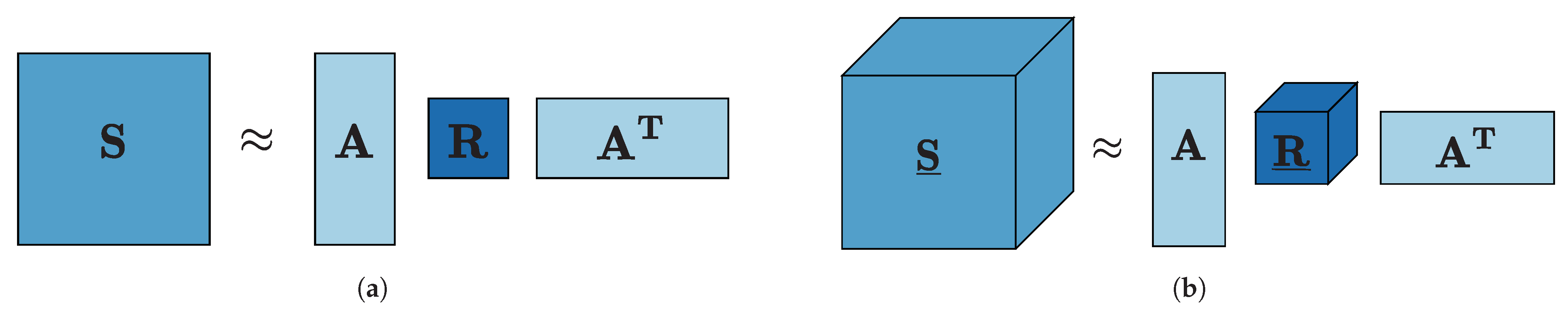
3. Constrained DEDICOM Models
3.1. The Row-Stochastic DEDICOM Model for Matrices
3.2. The Constrained DEDICOM Model for Tensors
3.3. On Symmetry
3.4. On Interpretability
4. Experiments and Results
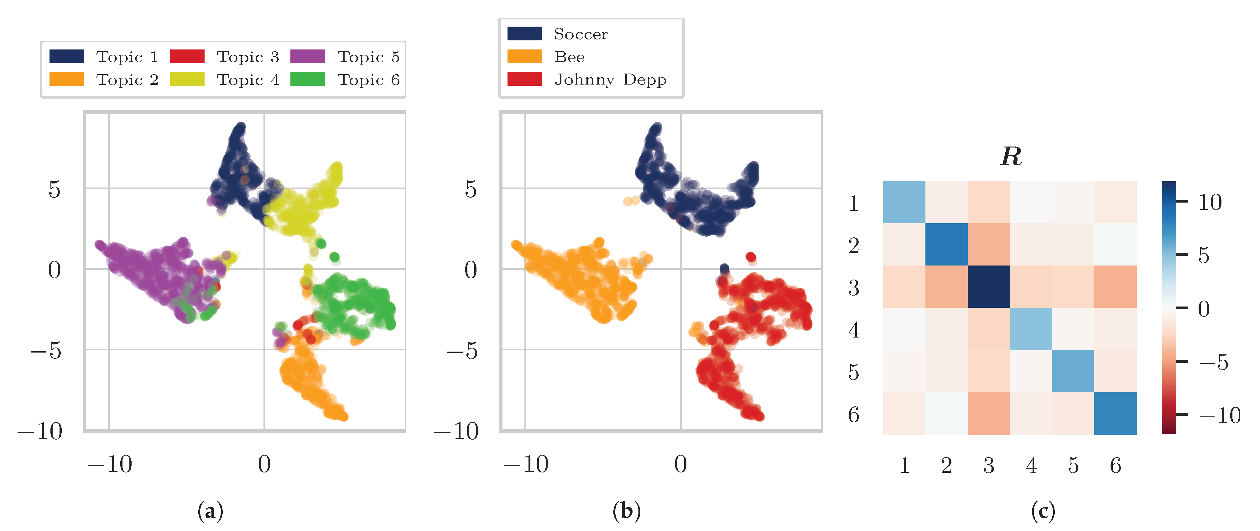
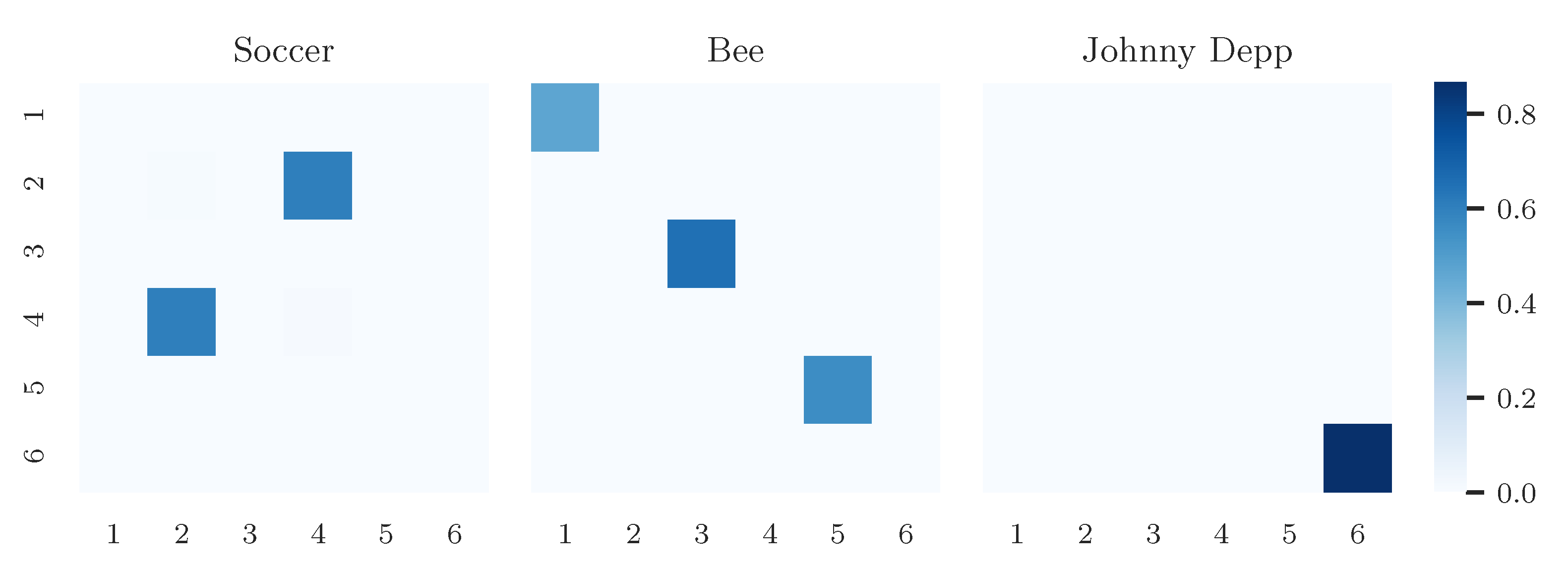
4.1. Data
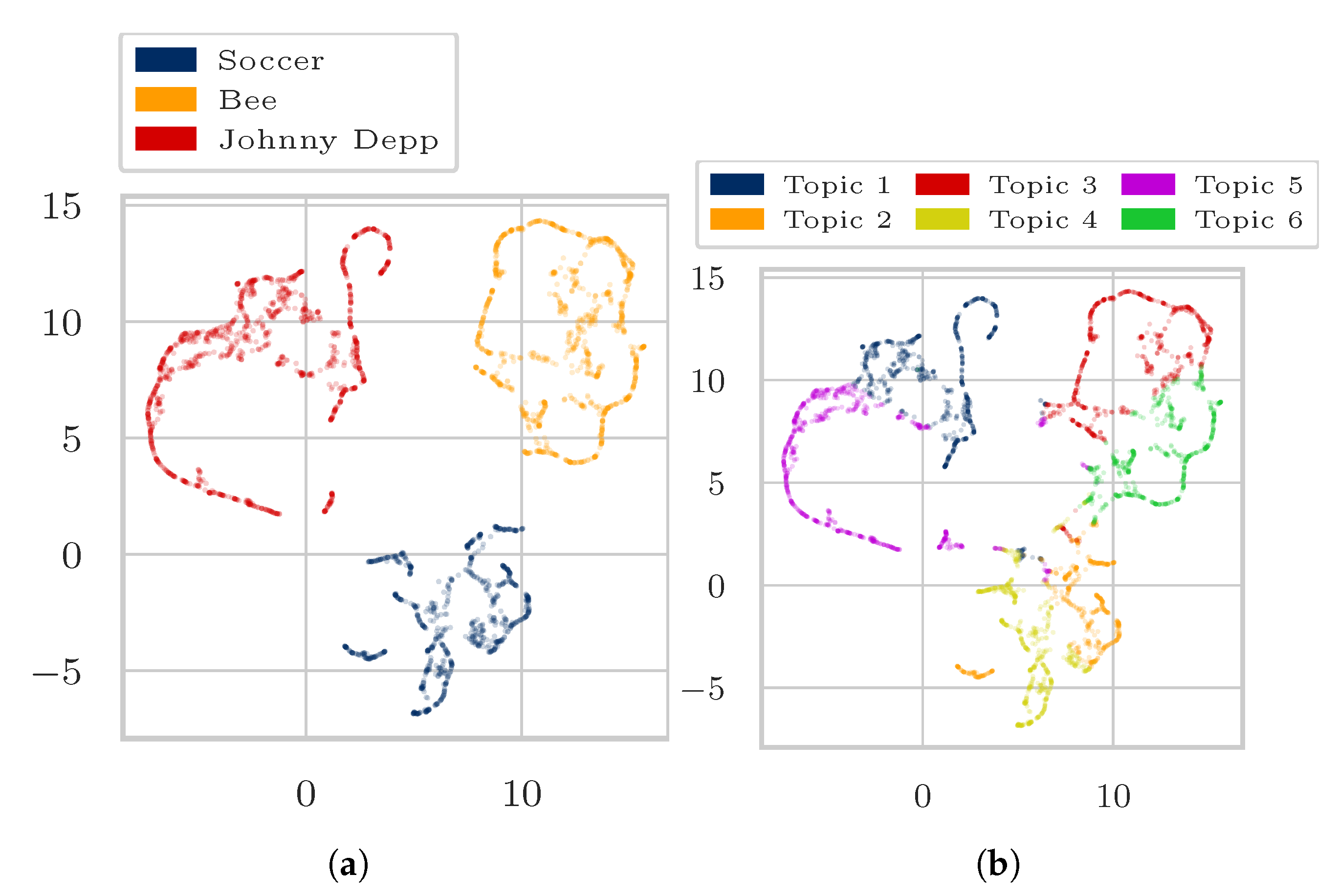
- “Soccer”, “Bee”, “Johnny Depp”,
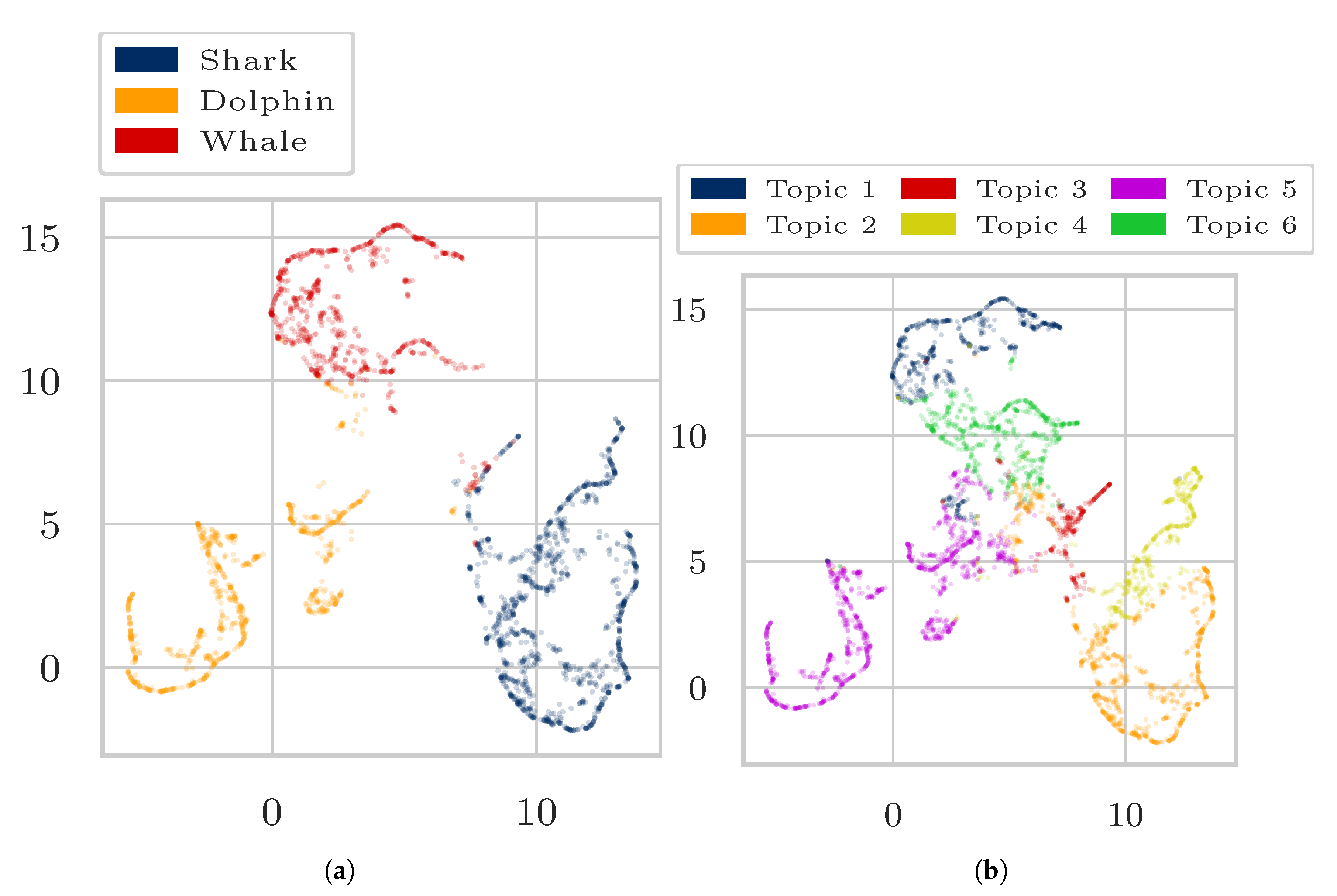
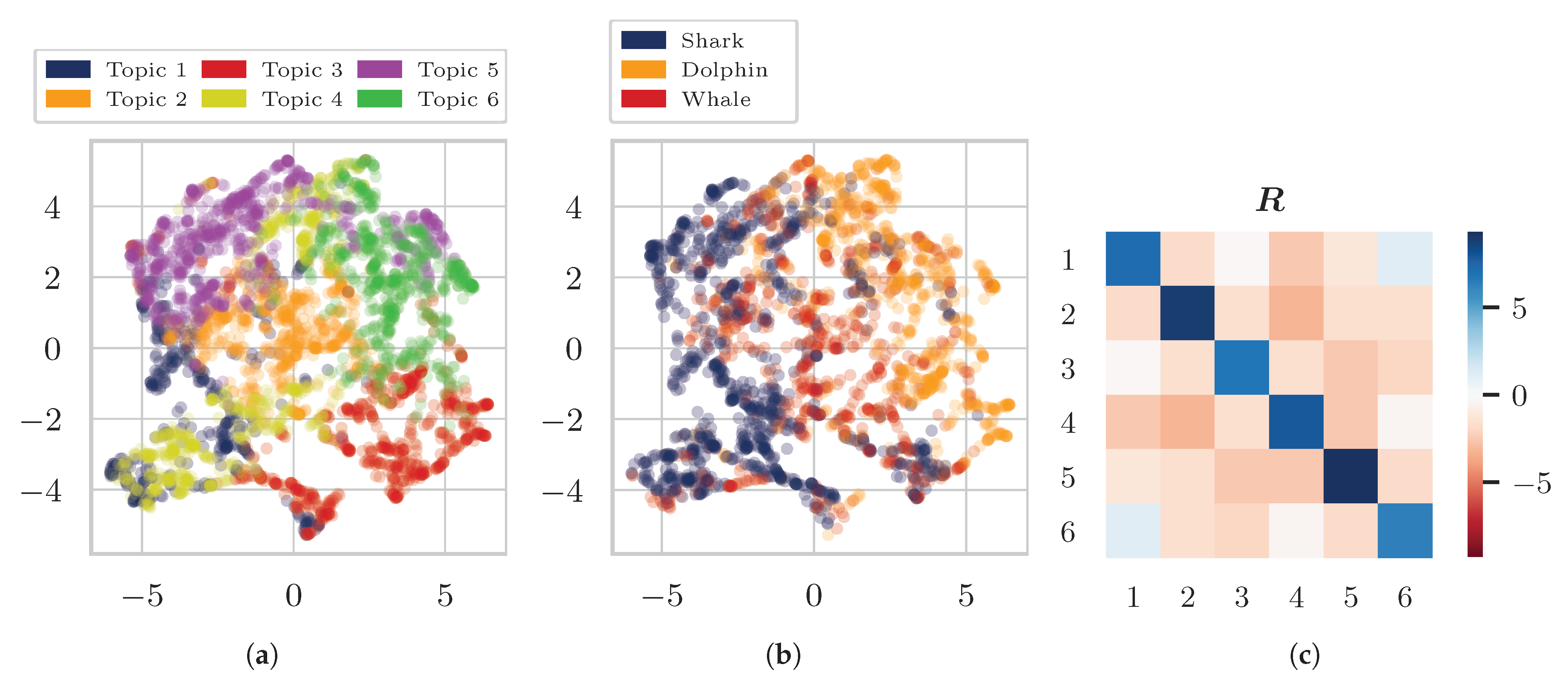
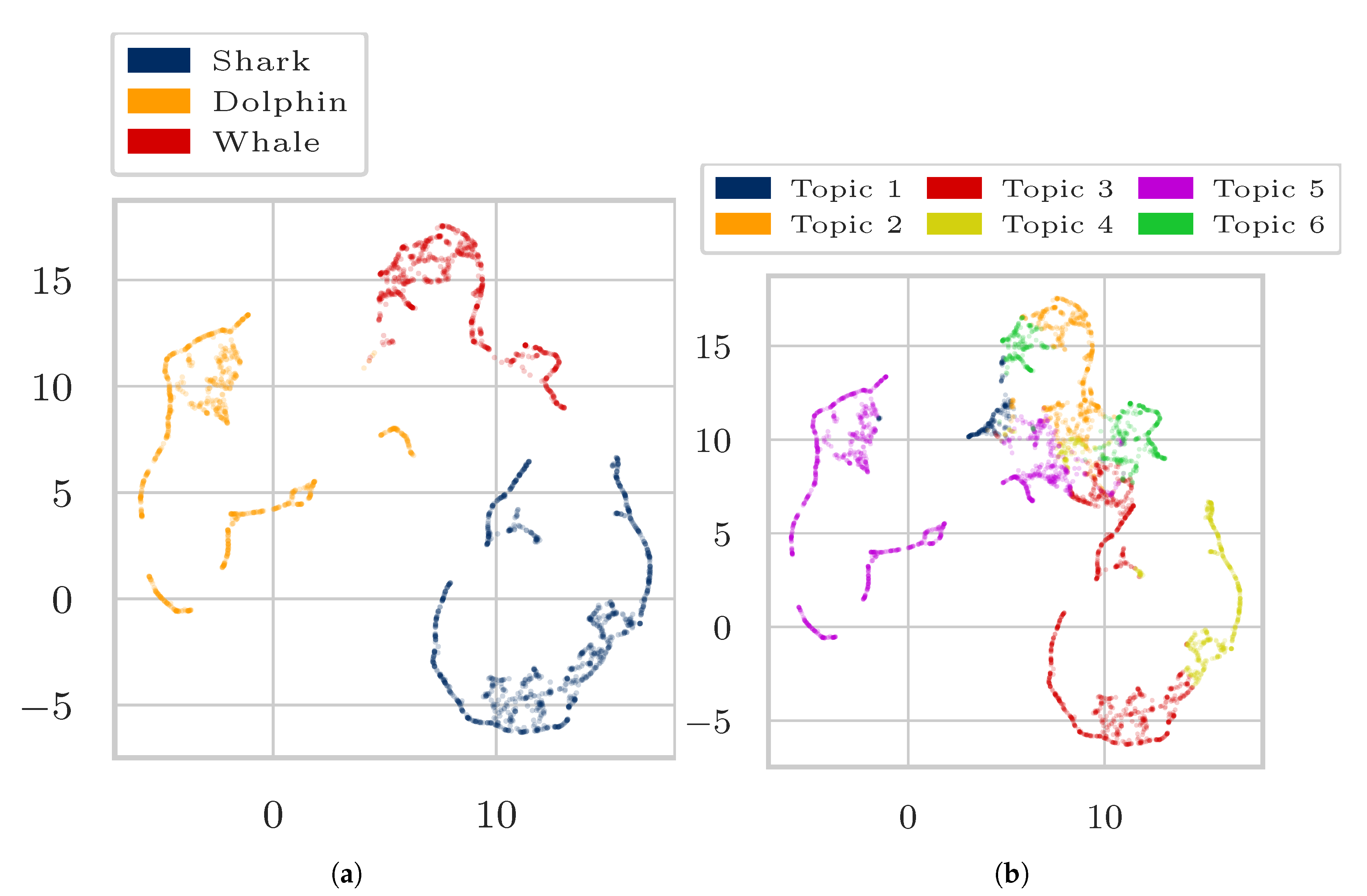
- “Dolphin”, “Shark”, “Whale”, and
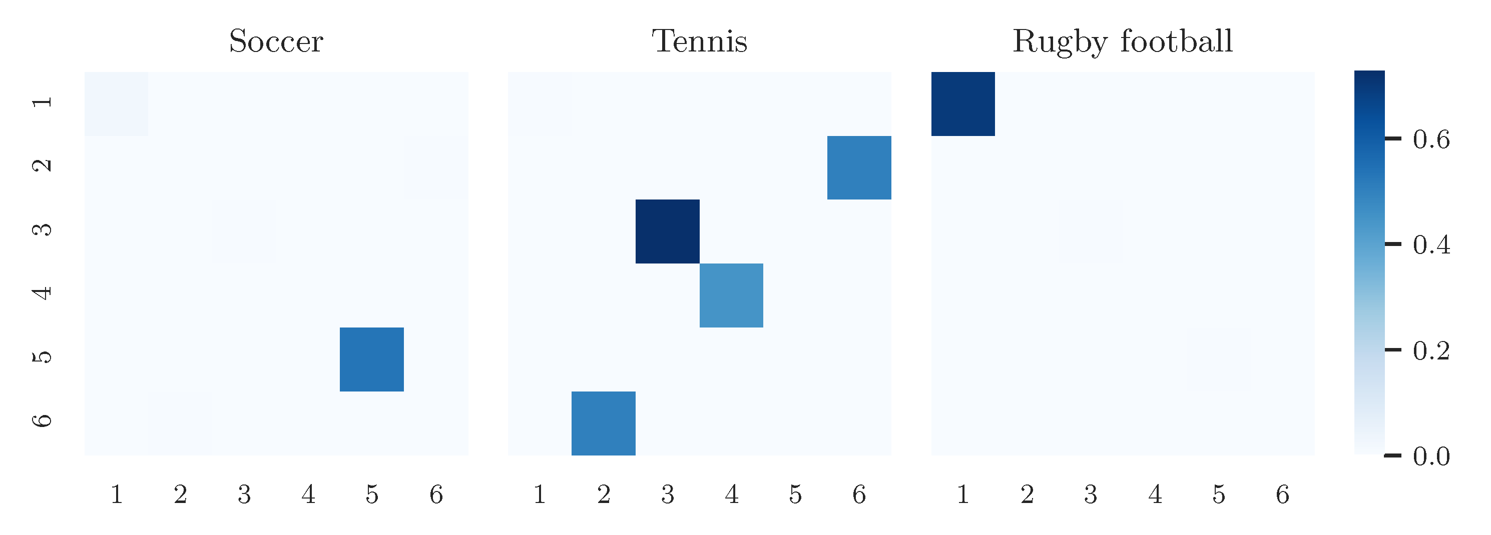
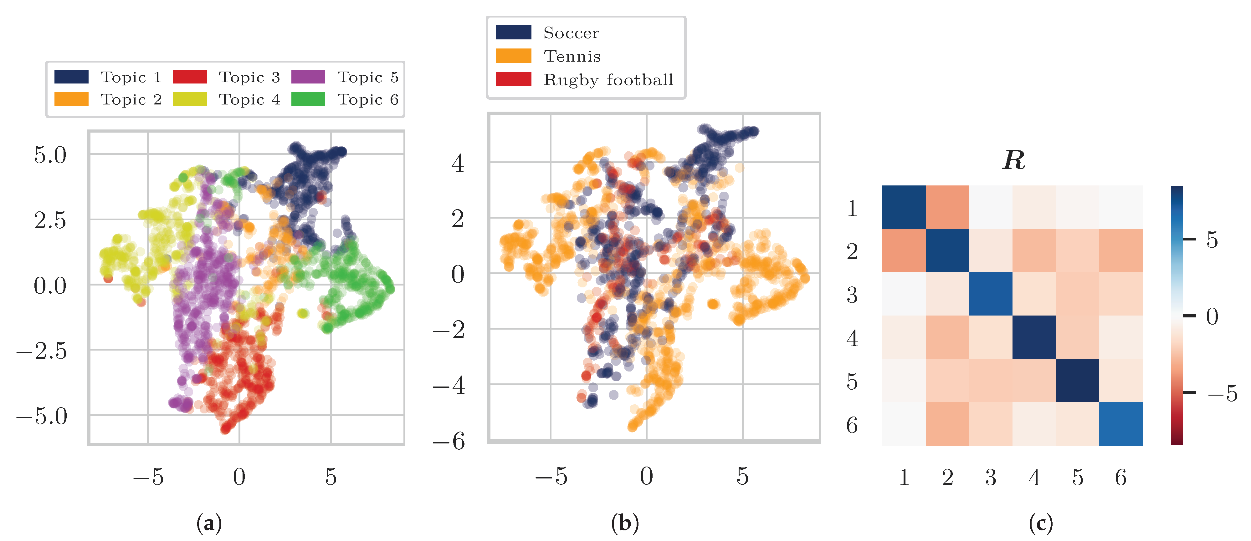
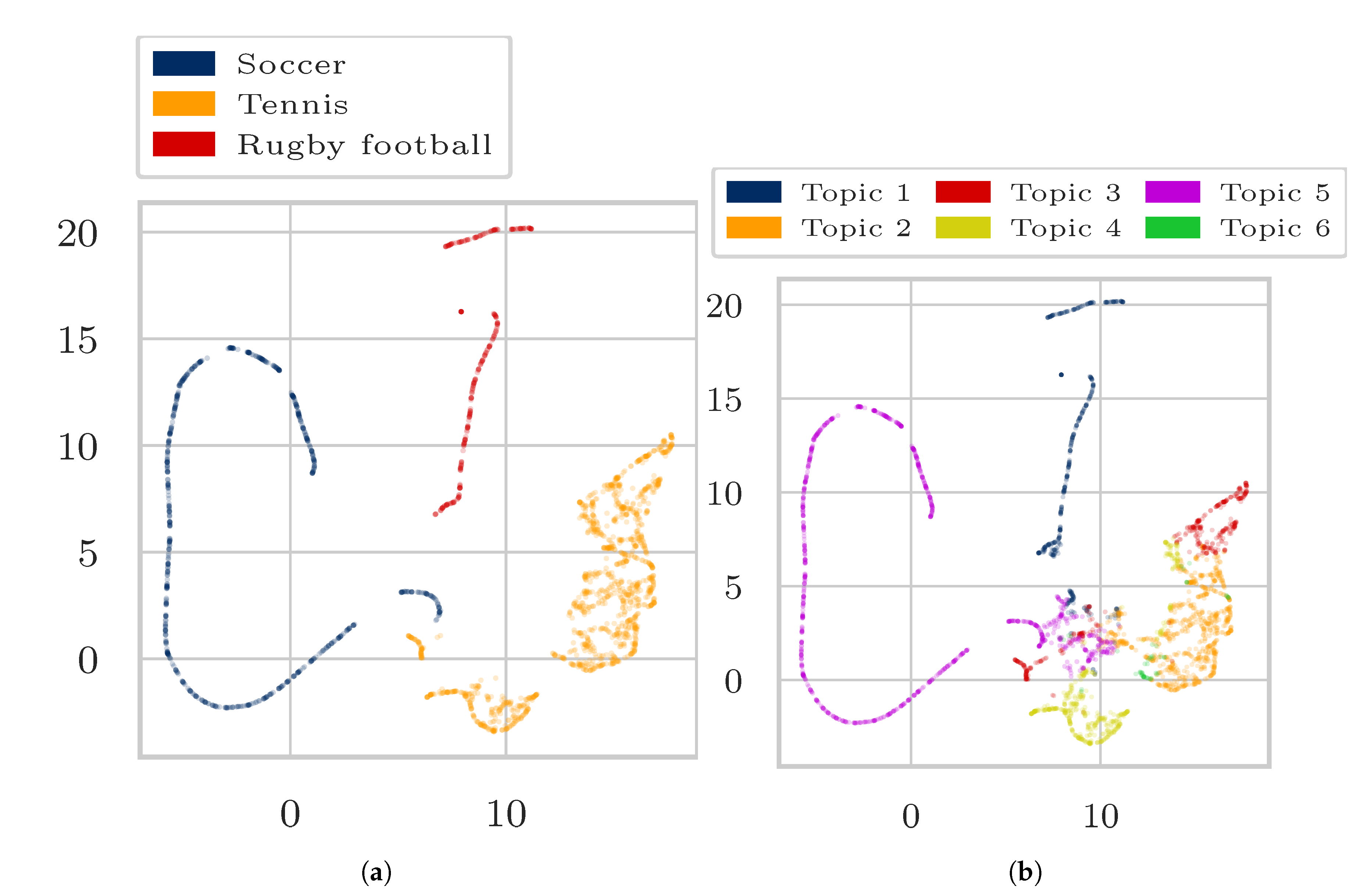
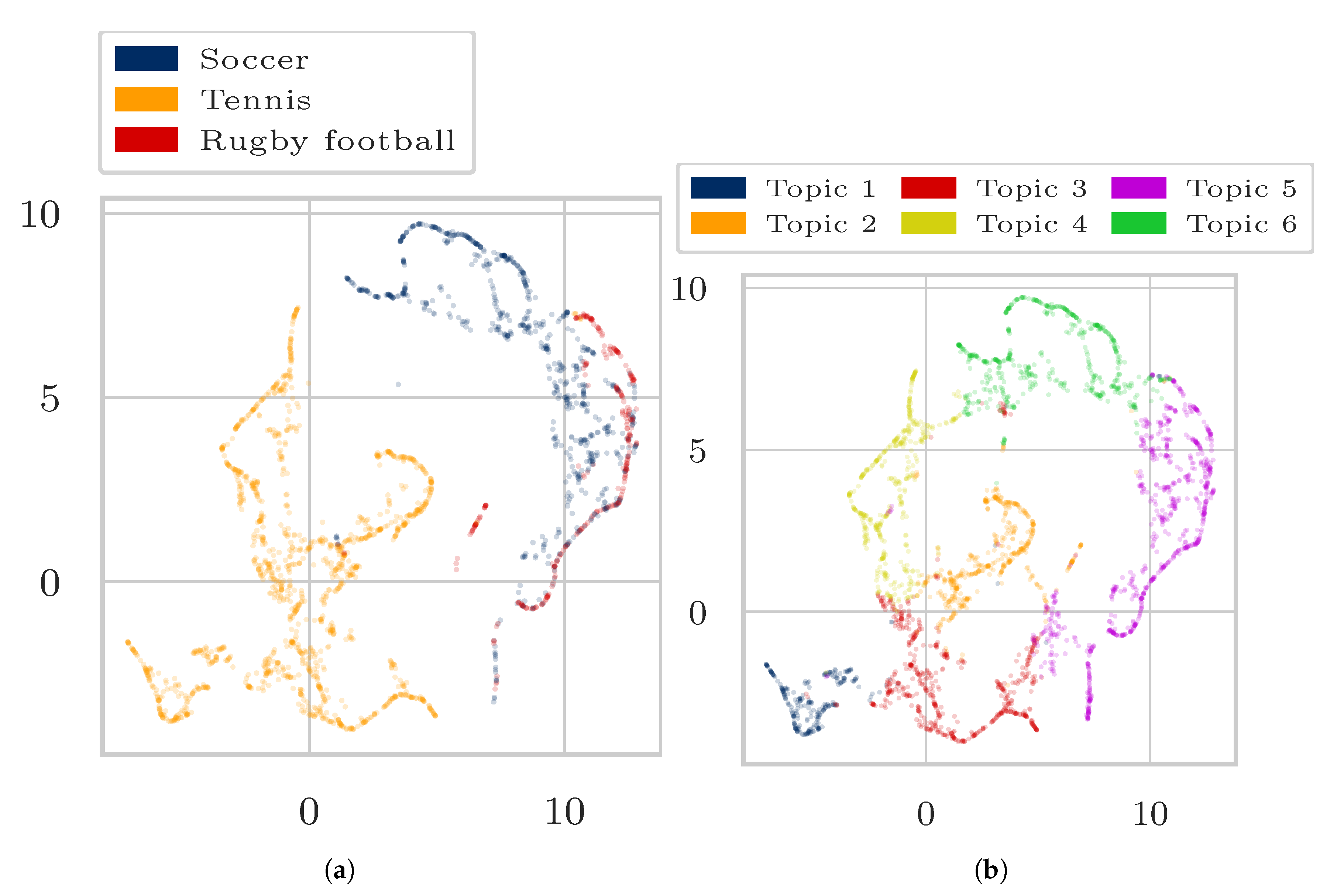
- “Soccer”, “Tennis”, “Rugby”.
4.2. Training
| Algorithm 1 The row-stochastic DEDICOM algorithm | |
| 1: initialize | ⊳See Equation (40) for the definition of |
| 2: initialize , , | ⊳Adam algorithm hyperparameters |
| 3: initialize , | ⊳Individual learning rates |
| 4: for i in , num_epochs do | |
| 5: Calculate loss | ⊳See Equation (7) |
| 6: | |
| 7: | |
| 8: return and R, where | ⊳See Equation (5) |
| Algorithm 2 The non-negative tensor DEDICOM algorithm | |
| 1: initialize | |
| 2: scale A by and by | ⊳See Equation (41) for the definitions of and |
| 3: for i in , num_epochs do | |
| 4: Calculate loss | ⊳See Equation (17) |
| 5: | |
| 6: | |
| 7: return A and | |
4.3. Results
5. Conclusions and Outlook
Author Contributions
Funding
Data Availability Statement
Conflicts of Interest
Appendix A. Additional Results
Appendix A.1. Additional Results on Wikipedia Data as Matrix Input

| Topic 1 | Topic 2 | Topic 3 | Topic 4 | Topic 5 | Topic 6 | ||
|---|---|---|---|---|---|---|---|
| NMF | #619 | #1238 | #628 | #595 | #612 | #389 | |
| 1 | ball | bees | film | football | heard | album | |
| 2 | may | species | starred | cup | depp | band | |
| 3 | penalty | bee | role | world | court | guitar | |
| 4 | referee | pollen | series | fifa | alcohol | vampires | |
| 5 | players | honey | burton | national | relationship | rock | |
| 6 | team | insects | character | association | stated | hollywood | |
| 7 | goal | food | films | international | divorce | song | |
| 8 | game | nests | box | women | abuse | released | |
| 9 | player | solitary | office | teams | paradis | perry | |
| 10 | play | eusocial | jack | uefa | stating | debut | |
| 0 | ball | bees | film | football | heard | album | |
| 1 | invoke | odors | burtondirected | athenaeus | crew | jones | |
| 2 | replaced | tufts | tone | paralympic | alleging | marilyn | |
| 3 | scores | colour | landau | governing | oped | roots | |
| 4 | subdivided | affected | brother | varieties | asserted | drums | |
| 0 | may | species | starred | cup | depp | band | |
| 1 | yd | niko | shared | inaugurated | refer | heroes | |
| 2 | ineffectiveness | commercially | whitaker | confederation | york | bowie | |
| 3 | tactical | microbiota | eccentric | gold | leaders | debut | |
| 4 | slower | strategies | befriends | headquarters | nonindian | solo | |
| LDA | #577 | #728 | #692 | #607 | #663 | #814 | |
| 1 | film | football | depp | penalty | bees | species | |
| 2 | series | women | children | heard | flowers | workers | |
| 3 | man | association | life | ball | bee | solitary | |
| 4 | played | fifa | role | direct | honey | players | |
| 5 | pirates | teams | starred | referee | pollen | colonies | |
| 6 | character | games | alongside | red | food | eusocial | |
| 7 | along | world | actor | time | increased | nest | |
| 8 | cast | cup | stated | goal | pollination | may | |
| 9 | also | game | burton | scored | times | size | |
| 10 | hollow | international | playing | player | larvae | egg | |
| 0 | film | football | depp | penalty | bees | species | |
| 1 | charlie | cup | critical | extra | bee | social | |
| 2 | near | canada | february | kicks | insects | chosen | |
| 3 | thinking | zealand | script | inner | authors | females | |
| 4 | shadows | activities | song | moving | hives | subspecies | |
| 0 | series | women | children | heard | flowers | workers | |
| 1 | crybaby | fifa | detective | allison | always | carcases | |
| 2 | waters | opera | crime | serious | eusociality | lived | |
| 3 | sang | exceeding | magazine | allergic | varroa | provisioned | |
| 4 | cast | cuju | barber | cost | wing | cuckoo | |
| SVD | #1228 | #797 | #628 | #369 | #622 | #437 | |
| 1 | bees | depp | game | cup | heard | beekeeping | |
| 2 | also | film | ball | football | court | increased | |
| 3 | bee | starred | team | fifa | divorce | honey | |
| 4 | species | role | players | world | stating | described | |
| 5 | played | series | penalty | european | alcohol | use | |
| 6 | time | burton | play | uefa | paradis | wild | |
| 7 | one | character | may | national | documents | varroa | |
| 8 | first | actor | referee | europe | abuse | mites | |
| 9 | two | released | competitions | continental | settlement | colony | |
| 10 | pollen | release | laws | confederation | sued | flowers | |
| 0 | bees | depp | game | cup | heard | beekeeping | |
| 1 | bee | iii | correct | continental | alleging | varroa | |
| 2 | develops | racism | abandoned | contested | attempting | animals | |
| 3 | studied | appropriation | maximum | confederations | finalized | mites | |
| 4 | crops | march | clear | conmebol | submitted | plato | |
| 0 | also | film | ball | football | court | increased | |
| 1 | although | waters | finely | er | declaration | usage | |
| 2 | told | robinson | poised | suffix | issued | farmers | |
| 3 | chosen | scott | worn | word | restraining | mentioned | |
| 4 | stars | costars | manner | appended | verbally | aeneid |
| Topic 1 #460 | Topic 2 #665 | Topic 3 #801 | Topic 4 #753 | Topic 5 #854 | Topic 6 #721 | |
|---|---|---|---|---|---|---|
| 1 | shark | calf | ship | conservation | water | dolphin |
| (0.665) | (0.428) | (0.459) | (0.334) | (0.416) | (0.691) | |
| 2 | sharks | months | became | countries | similar | dolphins |
| (0.645) | (0.407) | (0.448) | (0.312) | (0.374) | (0.655) | |
| 3 | fins | calves | poseidon | government | tissue | captivity |
| (0.487) | (0.407) | (0.44) | (0.309) | (0.373) | (0.549) | |
| 4 | killed | females | riding | wales | body | wild |
| (0.454) | (0.399) | (0.426) | (0.304) | (0.365) | (0.467) | |
| 5 | million | blubber | dionysus | bycatch | swimming | behavior |
| (0.451) | (0.374) | (0.422) | (0.29) | (0.357) | (0.461) | |
| 6 | fish | young | ancient | cancelled | blood | bottlenose |
| (0.448) | (0.37) | (0.42) | (0.288) | (0.346) | (0.453) | |
| 7 | international | sperm | deity | eastern | surface | sometimes |
| (0.442) | (0.356) | (0.412) | (0.287) | (0.344) | (0.449) | |
| 8 | fin | born | ago | policy | oxygen | human |
| (0.421) | (0.355) | (0.398) | (0.286) | (0.34) | (0.421) | |
| 9 | fishing | feed | melicertes | control | system | less |
| (0.405) | (0.349) | (0.395) | (0.285) | (0.336) | (0.42) | |
| 10 | teeth | mysticetes | greeks | imminent | swim | various |
| (0.398) | (0.341) | (0.394) | (0.282) | (0.336) | (0.418) | |
| 0 | shark | calf | ship | conservation | water | dolphin |
| (1.0) | (1.0) | (1.0) | (1.0) | (1.0) | (1.0) | |
| 2 | sharks | calves | dionysus | south | prey | dolphins |
| (0.981) | (0.978) | (0.995) | (0.981) | (0.964) | (0.925) | |
| 3 | fins | females | riding | states | swimming | sometimes |
| (0.958) | (0.976) | (0.992) | (0.981) | (0.959) | (0.909) | |
| 4 | killed | months | deity | united | allows | another |
| (0.929) | (0.955) | (0.992) | (0.978) | (0.957) | (0.904) | |
| 5 | fishing | young | poseidon | endangered | swim | bottlenose |
| (0.916) | (0.948) | (0.987) | (0.976) | (0.947) | (0.903) | |
| 0 | sharks | months | became | countries | similar | dolphins |
| (1.0) | (1.0) | (1.0) | (1.0) | (1.0) | (1.0) | |
| 2 | shark | born | old | eastern | surface | behavior |
| (0.981) | (0.992) | (0.953) | (0.991) | (0.992) | (0.956) | |
| 3 | fins | young | later | united | brain | sometimes |
| (0.936) | (0.992) | (0.946) | (0.989) | (0.97) | (0.945) | |
| 4 | tiger | sperm | ago | caught | sound | various |
| (0.894) | (0.985) | (0.939) | (0.987) | (0.968) | (0.943) | |
| 5 | killed | calves | modern | south | object | less |
| (0.887) | (0.984) | (0.937) | (0.979) | (0.965) | (0.937) |
| Topic 1 | Topic 2 | Topic 3 | Topic 4 | Topic 5 | Topic 6 | ||
|---|---|---|---|---|---|---|---|
| NMF | #492 | #907 | #452 | #854 | #911 | #638 | |
| 1 | blood | international | evidence | sonar | ago | calf | |
| 2 | body | killed | selfawareness | may | teeth | young | |
| 3 | heart | states | ship | surface | million | females | |
| 4 | gills | conservation | dionysus | clicks | mysticetes | captivity | |
| 5 | bony | new | came | prey | whales | calves | |
| 6 | oxygen | united | another | use | years | months | |
| 7 | organs | shark | important | underwater | baleen | born | |
| 8 | tissue | world | poseidon | sounds | cetaceans | species | |
| 9 | water | endangered | mark | known | modern | male | |
| 10 | via | islands | riding | similar | extinct | female | |
| 0 | blood | international | evidence | sonar | ago | calf | |
| 1 | travels | proposal | flaws | poisoned | consist | uninformed | |
| 2 | enters | lipotidae | methodological | signals | specialize | primary | |
| 3 | vibration | banned | nictating | ≈– | legs | born | |
| 4 | tolerant | iniidae | wake | emitted | closest | leaner | |
| 0 | body | killed | selfawareness | may | teeth | young | |
| 1 | crystal | law | legendary | individuals | fuel | brood | |
| 2 | blocks | consumers | humankind | helping | lamp | lacking | |
| 3 | modified | pontoporiidae | helpers | waste | filterfeeding | accurate | |
| 4 | slits | org | performing | depression | krill | consistency | |
| LDA | #650 | #785 | #695 | #815 | #635 | #674 | |
| 1 | killed | teeth | head | species | meat | air | |
| 2 | system | baleen | fish | male | whale | using | |
| 3 | endangered | mysticetes | dolphin | females | ft | causing | |
| 4 | often | ago | fin | whales | fisheries | currents | |
| 5 | close | jaw | eyes | sometimes | also | sounds | |
| 6 | sharks | family | fat | captivity | ocean | groups | |
| 7 | countries | water | navy | young | threats | sound | |
| 8 | since | includes | popular | shark | children | research | |
| 9 | called | allow | tissue | female | population | clicks | |
| 10 | vessels | greater | tail | wild | bottom | burst | |
| 0 | killed | teeth | head | species | meat | air | |
| 1 | postures | dense | underside | along | porbeagle | australis | |
| 2 | dolphinariums | cetacea | grooves | another | source | submerged | |
| 3 | town | tourism | eyesight | long | activities | melbourne | |
| 4 | onethird | planktonfeeders | osmoregulation | sleep | comparable | spear | |
| 0 | system | baleen | fish | male | whale | using | |
| 1 | dominate | mysticetes | mostly | females | live | communication | |
| 2 | close | distinguishing | swim | aorta | human | become | |
| 3 | controversy | unique | due | female | cold | associated | |
| 4 | agree | remove | whole | position | parts | mirror | |
| SVD | #1486 | #544 | #605 | #469 | #539 | #611 | |
| 1 | dolphins | water | shark | million | poseidon | dolphin | |
| 2 | species | body | sharks | years | became | meat | |
| 3 | whales | tail | fins | ago | ship | family | |
| 4 | fish | teeth | international | whale | riding | river | |
| 5 | also | flippers | killed | two | evidence | similar | |
| 6 | large | tissue | fishing | calf | melicertes | extinct | |
| 7 | may | allows | fin | mya | deity | called | |
| 8 | one | air | law | later | ino | used | |
| 9 | animals | feed | new | months | came | islands | |
| 10 | use | bony | conservation | mysticetes | made | genus | |
| 0 | dolphins | water | shark | million | poseidon | dolphin | |
| 1 | various | vertical | corpse | approximately | games | depicted | |
| 2 | finding | unlike | stocks | assigned | phalanthus | makara | |
| 3 | military | chew | galea | hybodonts | statue | capensis | |
| 4 | selfmade | lack | galeomorphii | appeared | isthmian | goddess | |
| 0 | species | body | sharks | years | became | meat | |
| 1 | herd | heart | mostly | acanthodians | pirates | contaminated | |
| 2 | reproduction | resisting | fda | spent | elder | harpoon | |
| 3 | afford | fit | lists | stretching | mistook | practitioner | |
| 4 | maturity | posterior | carcharias | informal | wealthy | pcbs |
| Topic 1 #539 | Topic 2 #302 | Topic 3 #563 | Topic 4 #635 | Topic 5 #650 | Topic 6 #530 | |
|---|---|---|---|---|---|---|
| 1 | may | leads | tournaments | greatest | football | net |
| (0.599) | (0.212) | (0.588) | (0.572) | (0.553) | (0.644) | |
| 2 | penalty | sole | tournament | tennis | rugby | shot |
| (0.576) | (0.205) | (0.517) | (0.497) | (0.542) | (0.629) | |
| 3 | referee | competes | events | female | south | stance |
| (0.564) | (0.205) | (0.509) | (0.44) | (0.484) | (0.553) | |
| 4 | team | extending | prize | ever | union | stroke |
| (0.517) | (0.204) | (0.501) | (0.433) | (0.47) | (0.543) | |
| 5 | goal | fixing | tour | navratilova | wales | serve |
| (0.502) | (0.203) | (0.497) | (0.405) | (0.459) | (0.537) | |
| 6 | kick | triggered | money | modern | national | rotation |
| (0.459) | (0.203) | (0.488) | (0.401) | (0.446) | (0.513) | |
| 7 | play | bleeding | cup | best | england | backhand |
| (0.455) | (0.202) | (0.486) | (0.4) | (0.438) | (0.508) | |
| 8 | ball | fraud | world | wingfield | new | hit |
| (0.452) | (0.202) | (0.467) | (0.394) | (0.416) | (0.507) | |
| 9 | offence | inflammation | atp | sports | europe | forehand |
| (0.444) | (0.202) | (0.464) | (0.39) | (0.406) | (0.499) | |
| 10 | foul | conditions | men | williams | states | torso |
| (0.443) | (0.201) | (0.463) | (0.389) | (0.404) | (0.487) | |
| 0 | may | leads | tournaments | greatest | football | net |
| (1.0) | (1.0) | (1.0) | (1.0) | (1.0) | (1.0) | |
| 2 | goal | tiredness | events | female | union | shot |
| (0.98) | (1.0) | (0.992) | (0.98) | (0.98) | (0.994) | |
| 3 | play | ineffectiveness | tour | ever | rugby | serve |
| (0.959) | (1.0) | (0.989) | (0.971) | (0.979) | (0.987) | |
| 4 | penalty | recommences | money | navratilova | association | hit |
| (0.954) | (1.0) | (0.986) | (0.967) | (0.96) | (0.984) | |
| 5 | team | mandated | prize | tennis | england | stance |
| (0.953) | (1.0) | (0.985) | (0.962) | (0.958) | (0.955) | |
| 0 | penalty | sole | tournament | tennis | rugby | shot |
| (1.0) | (1.0) | (1.0) | (1.0) | (1.0) | (1.0) | |
| 2 | referee | discretion | events | greatest | football | net |
| (0.985) | (1.0) | (0.98) | (0.962) | (0.979) | (0.994) | |
| 3 | kick | synonym | event | female | union | serve |
| (0.985) | (1.0) | (0.978) | (0.953) | (0.975) | (0.987) | |
| 4 | offence | violated | atp | year | england | hit |
| (0.982) | (1.0) | (0.974) | (0.951) | (0.961) | (0.983) | |
| 5 | foul | layout | money | navratilova | wales | stance |
| (0.982) | (1.0) | (0.966) | (0.949) | (0.949) | (0.98) |
| Topic 1 | Topic 2 | Topic 3 | Topic 4 | Topic 5 | Topic 6 | ||
|---|---|---|---|---|---|---|---|
| NMF | #511 | #453 | #575 | #657 | #402 | #621 | |
| 1 | net | referee | national | tournaments | rackets | rules | |
| 2 | shot | penalty | south | doubles | balls | wingfield | |
| 3 | serve | may | football | singles | made | december | |
| 4 | hit | kick | cup | events | size | game | |
| 5 | stance | card | europe | tour | must | sports | |
| 6 | stroke | listed | fifa | prize | strings | lawn | |
| 7 | backhand | foul | union | money | standard | modern | |
| 8 | ball | misconduct | wales | atp | synthetic | greek | |
| 9 | server | red | africa | men | leather | fa | |
| 10 | service | offence | new | grand | width | first | |
| 0 | net | referee | national | tournaments | rackets | rules | |
| 1 | defensive | retaken | serbia | bruno | pressurisation | collection | |
| 2 | closer | interference | gold | woodies | become | hourglass | |
| 3 | somewhere | dismissed | north | eliminated | equivalents | unhappy | |
| 4 | center | fully | headquarters | soares | size | originated | |
| 0 | shot | penalty | south | doubles | balls | wingfield | |
| 1 | rotated | prior | asian | combining | express | experimenting | |
| 2 | execute | yellow | argentina | becker | oz | llanelidan | |
| 3 | strive | duration | la | exclusively | bladder | attended | |
| 4 | curve | primary | kong | woodbridge | length | antiphanes | |
| LDA | #413 | #518 | #395 | #776 | #616 | #501 | |
| 1 | used | net | wimbledon | world | penalty | clubs | |
| 2 | forehand | ball | episkyros | cup | score | rugby | |
| 3 | use | serve | occurs | tournaments | goal | schools | |
| 4 | large | shot | grass | football | team | navratilova | |
| 5 | notable | opponent | roman | fifa | end | forms | |
| 6 | also | hit | bc | national | players | playing | |
| 7 | western | lines | occur | international | match | sport | |
| 8 | twohanded | server | ad | europe | goals | greatest | |
| 9 | doubles | service | island | tournament | time | union | |
| 10 | injury | may | believed | states | scored | war | |
| 0 | used | net | wimbledon | world | penalty | clubs | |
| 1 | seconds | mistaken | result | british | measure | sees | |
| 2 | restrictions | diagonal | determined | cancelled | crossed | papua | |
| 3 | although | hollow | exists | combined | requiring | admittance | |
| 4 | use | perpendicular | win | wii | teammate | forces | |
| 0 | forehand | ball | episkyros | cup | score | rugby | |
| 1 | twohanded | long | roman | multiple | penalty | union | |
| 2 | grips | deuce | bc | inline | bar | public | |
| 3 | facetiously | position | island | fifa | fouled | took | |
| 4 | woodbridge | allows | believed | manufactured | hour | published | |
| SVD | #1310 | #371 | #423 | #293 | #451 | #371 | |
| 1 | players | net | tournaments | stroke | greatest | balls | |
| 2 | player | ball | singles | forehand | ever | rackets | |
| 3 | tennis | shot | doubles | stance | female | size | |
| 4 | also | serve | tour | power | wingfield | square | |
| 5 | play | opponent | slam | backhand | williams | made | |
| 6 | football | may | prize | torso | navratilova | leather | |
| 7 | team | hit | money | grip | game | weight | |
| 8 | first | service | grand | rotation | said | standard | |
| 9 | one | hitting | events | twohanded | serena | width | |
| 10 | rugby | line | ranking | used | sports | past | |
| 0 | players | net | tournaments | stroke | greatest | balls | |
| 1 | breaking | pace | masters | rotates | lived | panels | |
| 2 | one | reach | lowest | achieve | female | sewn | |
| 3 | running | underhand | events | face | biggest | entire | |
| 4 | often | air | tour | adds | potential | leather | |
| 0 | player | ball | singles | forehand | ever | rackets | |
| 1 | utilize | keep | indian | twohanded | autobiography | meanwhile | |
| 2 | give | hands | doubles | begins | jack | laminated | |
| 3 | converted | pass | pro | backhand | consistent | wood | |
| 4 | touch | either | rankings | achieve | gonzales | strings |
Appendix A.2. Additional Results on Wikipedia Data as Tensor Input


| Topic 1 #226 | Topic 2 #628 | Topic 3 #1048 | Topic 4 #571 | Topic 5 #1267 | Topic 6 #554 | |
|---|---|---|---|---|---|---|
| 1 | cells | mysticetes | shark | bony | dolphin | whaling |
| (1.785) | (1.808) | (3.019) | (1.621) | (3.114) | (3.801) | |
| 2 | brain | whales | sharks | blood | dolphins | iwc |
| (1.624) | (1.791) | (2.737) | (1.452) | (2.908) | (2.159) | |
| 3 | light | feed | fins | fish | bottlenose | aboriginal |
| (1.561) | (1.427) | (1.442) | (1.438) | (1.629) | (2.098) | |
| 4 | cone | baleen | killed | gills | meat | canada |
| (1.448) | (1.33) | (1.407) | (1.206) | (1.403) | (1.912) | |
| 5 | allow | odontocetes | endangered | teeth | behavior | moratorium |
| (1.32) | (1.278) | (1.377) | (1.088) | (1.399) | (1.867) | |
| 6 | greater | consist | hammerhead | body | captivity | industry |
| (1.292) | (1.162) | (1.269) | (1.043) | (1.298) | (1.855) | |
| 7 | slightly | water | conservation | system | river | us |
| (1.269) | (1.096) | (1.227) | (1.027) | (1.281) | (1.838) | |
| 8 | ear | krill | trade | skeleton | common | belugas |
| (1.219) | (1.05) | (1.226) | (1.008) | (1.275) | (1.585) | |
| 9 | cornea | toothed | whitetip | called | selfawareness | whale |
| (1.158) | (1.003) | (1.203) | (0.99) | (1.248) | (1.542) | |
| 10 | rod | sperm | finning | tissue | often | gb£ |
| (1.128) | (0.991) | (1.184) | (0.875) | (1.218) | (1.528) |
| Topic 1 | Topic 2 | Topic 3 | Topic 4 | Topic 5 | Topic 6 | |
|---|---|---|---|---|---|---|
| 0 | cells | mysticetes | shark | bony | dolphin | whaling |
| (1.0) | (1.0) | (1.0) | (1.0) | (1.0) | (1.0) | |
| 1 | sensitive | unborn | native | edges | hybrid | māori |
| (1.0) | (1.0) | (1.0) | (1.0) | (1.0) | (1.0) | |
| 2 | cone | grind | tl | mirabile | hybridization | trips |
| (1.0) | (1.0) | (1.0) | (1.0) | (1.0) | (1.0) | |
| 3 | rod | counterparts | predators—organisms | matches | yangtze | predominantly |
| (0.998) | (1.0) | (1.0) | (1.0) | (1.0) | (1.0) | |
| 4 | corneas | threechambered | cretaceous | turbulence | grampus | revenue |
| (0.998) | (1.0) | (1.0) | (1.0) | (1.0) | (1.0) | |
| 0 | brain | whales | sharks | blood | dolphins | iwc |
| (1.0) | (1.0) | (1.0) | (1.0) | (1.0) | (1.0) | |
| 1 | receive | extended | reminiscent | hydrodynamic | superpod | distinction |
| (0.998) | (0.996) | (1.0) | (0.998) | (1.0) | (1.0) | |
| 2 | equalizer | bryde | electrical | scattering | masturbation | billion |
| (0.998) | (0.996) | (1.0) | (0.998) | (1.0) | (1.0) | |
| 3 | lobes | closes | induced | reminder | interaction | spain |
| (0.997) | (0.996) | (1.0) | (0.998) | (1.0) | (1.0) | |
| 4 | clear | effects | coarsely | flows | stressful | competition |
| (0.997) | (0.996) | (1.0) | (0.998) | (1.0) | (1.0) |


| Topic 1 #441 | Topic 2 #861 | Topic 3 #412 | Topic 4 #482 | Topic 5 #968 | Topic 6 #57 | |
|---|---|---|---|---|---|---|
| 1 | rugby | titles | rackets | net | penalty | doubles |
| (2.55) | (1.236) | (2.176) | (2.767) | (1.721) | (2.335) | |
| 2 | union | wta | wingfield | shot | football | singles |
| (2.227) | (1.196) | (1.536) | (2.586) | (1.701) | (2.321) | |
| 3 | wales | circuit | modern | serve | team | tournaments |
| (1.822) | (1.123) | (1.513) | (2.393) | (1.507) | (2.245) | |
| 4 | georgia | futures | racket | hit | laws | tennis |
| (1.682) | (1.122) | (1.43) | (1.978) | (1.462) | (1.752) | |
| 5 | fiji | earn | th | stance | referee | grand |
| (1.557) | (1.104) | (1.355) | (1.945) | (1.449) | (1.662) | |
| 6 | samoa | offer | lawn | service | fifa | events |
| (1.474) | (1.096) | (1.316) | (1.83) | (1.439) | (1.648) | |
| 7 | zealand | mixed | century | stroke | may | slam |
| (1.458) | (1.089) | (1.236) | (1.797) | (1.435) | (1.623) | |
| 8 | new | draws | strings | server | goal | player |
| (1.414) | (1.085) | (1.179) | (1.761) | (1.353) | (1.344) | |
| 9 | tonga | atp | yielded | backhand | competitions | professional |
| (1.374) | (1.072) | (1.121) | (1.692) | (1.345) | (1.328) | |
| 10 | south | challenger | balls | forehand | associations | players |
| (1.369) | (1.07) | (1.101) | (1.554) | (1.288) | (1.316) |
| Topic 1 | Topic 2 | Topic 3 | Topic 4 | Topic 5 | Topic 6 | |
|---|---|---|---|---|---|---|
| 0 | rugby | titles | rackets | net | penalty | doubles |
| (1.0) | (1.0) | (1.0) | (1.0) | (1.0) | (1.0) | |
| 1 | ireland | hopman | proximal | hit | organisers | singles |
| (1.0) | (1.0) | (1.0) | (1.0) | (1.0) | (1.0) | |
| 2 | union | dress | interlaced | formally | elapsed | tournaments |
| (1.0) | (1.0) | (1.0) | (1.0) | (1.0) | (0.985) | |
| 3 | backfired | tennischannel | harry | offensive | polite | grand |
| (1.0) | (0.998) | (1.0) | (1.0) | (1.0) | (0.975) | |
| 4 | kilopascals | seoul | deserves | deeply | modest | slam |
| (1.0) | (0.998) | (1.0) | (1.0) | (1.0) | (0.971) | |
| 0 | union | wta | wingfield | shot | football | singles |
| (1.0) | (1.0) | (1.0) | (1.0) | (1.0) | (1.0) | |
| 1 | rugby | helps | proximal | requires | circumference | doubles |
| (1.0) | (1.0) | (1.0) | (1.0) | (1.0) | (1.0) | |
| 2 | ireland | hamilton | interlaced | backwards | touchline | tournaments |
| (1.0) | (1.0) | (1.0) | (1.0) | (1.0) | (0.985) | |
| 3 | backfired | weeks | harry | entail | sanctions | grand |
| (1.0) | (1.0) | (1.0) | (1.0) | (1.0) | (0.975) | |
| 4 | zealand | couple | deserves | torso | home | slam |
| (1.0) | (1.0) | (1.0) | (1.0) | (0.999) | (0.971) |
| Topic 1 #275 | Topic 2 #505 | Topic 3 #607 | Topic 4 #459 | Topic 5 #816 | Topic 6 #559 | |
|---|---|---|---|---|---|---|
| 1 | greatest | rackets | tournaments | net | football | penalty |
| (39.36) | (33.707) | (29.126) | (29.789) | (27.534) | (27.793) | |
| 2 | ever | modern | events | shot | rugby | referee |
| (26.587) | (24.281) | (25.327) | (27.947) | (24.037) | (23.632) | |
| 3 | female | balls | tour | serve | union | goal |
| (25.52) | (22.016) | (23.488) | (25.722) | (21.397) | (23.072) | |
| 4 | navratilova | wingfield | prize | hit | south | may |
| (24.348) | (20.923) | (21.823) | (21.344) | (20.761) | (22.978) | |
| 5 | best | tennis | atp | stance | national | team |
| (24.114) | (19.863) | (21.124) | (20.75) | (19.586) | (21.258) | |
| 6 | williams | strings | money | service | fifa | kick |
| (22.207) | (18.602) | (20.667) | (19.7) | (19.331) | (21.052) | |
| 7 | serena | racket | doubles | server | wales | foul |
| (21.256) | (18.369) | (19.919) | (19.051) | (18.627) | (19.018) | |
| 8 | said | made | ranking | stroke | league | listed |
| (20.666) | (17.622) | (19.736) | (18.781) | (18.31) | (17.736) | |
| 9 | martina | yielded | us | backhand | cup | free |
| (20.153) | (17.284) | (19.431) | (17.809) | (17.015) | (17.702) | |
| 10 | budge | th | masters | ball | association | goals |
| (20.111) | (16.992) | (18.596) | (17.2) | (16.721) | (17.209) |
| Topic 1 | Topic 2 | Topic 3 | Topic 4 | Topic 5 | Topic 6 | |
|---|---|---|---|---|---|---|
| 0 | greatest | rackets | tournaments | net | football | penalty |
| (1.0) | (1.0) | (1.0) | (1.0) | (1.0) | (1.0) | |
| 1 | illustrated | garden | us | lob | midlothian | whole |
| (1.0) | (1.0) | (1.0) | (1.0) | (1.0) | (1.0) | |
| 2 | johansson | construction | earned | receiving | alcock | corner |
| (1.0) | (1.0) | (1.0) | (1.0) | (1.0) | (1.0) | |
| 3 | wilton | yielded | participating | rotates | capital | offender |
| (1.0) | (1.0) | (1.0) | (1.0) | (1.0) | (1.0) | |
| 4 | jonathan | energy | receives | adds | representatives | stoke |
| (1.0) | (1.0) | (1.0) | (1.0) | (1.0) | (1.0) | |
| 0 | ever | modern | events | shot | rugby | referee |
| (1.0) | (1.0) | (1.0) | (1.0) | (1.0) | (1.0) | |
| 1 | deserved | design | juniors | lobber | slang | dismissed |
| (1.0) | (0.999) | (1.0) | (1.0) | (1.0) | (1.0) | |
| 2 | stated | version | bowl | unable | colonists | showing |
| (1.0) | (0.999) | (1.0) | (1.0) | (1.0) | (1.0) | |
| 3 | female | shape | comprised | alter | sevenaside | stoppage |
| (1.0) | (0.998) | (1.0) | (1.0) | (1.0) | (1.0) | |
| 4 | contemporaries | stitched | carlo | applying | seldom | layout |
| (1.0) | (0.998) | (1.0) | (1.0) | (1.0) | (1.0) |
| Topic 1 #675 | Topic 2 #996 | Topic 3 #279 | Topic 4 #491 | Topic 5 #1190 | Topic 6 #663 | |
|---|---|---|---|---|---|---|
| 1 | whaling | sharks | young | killed | dolphin | mysticetes |
| (34.584) | (30.418) | (33.823) | (23.214) | (35.52) | (24.404) | |
| 2 | whale | fish | born | shark | dolphins | flippers |
| (25.891) | (23.648) | (27.62) | (22.6) | (31.881) | (22.059) | |
| 3 | whales | bony | oviduct | states | bottlenose | odontocetes |
| (21.653) | (19.689) | (23.706) | (21.24) | (18.198) | (21.621) | |
| 4 | belugas | prey | viviparity | endangered | behavior | water |
| (20.933) | (18.785) | (23.694) | (20.976) | (18.003) | (21.087) | |
| 5 | aboriginal | teeth | embryos | conservation | selfawareness | tail |
| (19.44) | (18.242) | (22.966) | (20.398) | (16.48) | (18.268) | |
| 6 | iwc | blood | continue | fins | meat | mya |
| (19.226) | (16.521) | (21.752) | (18.641) | (16.02) | (17.79) | |
| 7 | canada | gills | calves | new | often | baleen |
| (18.691) | (13.34) | (21.25) | (18.445) | (15.687) | (17.189) | |
| 8 | arctic | tissue | blubber | international | captivity | limbs |
| (17.406) | (12.927) | (21.094) | (18.4) | (15.452) | (16.56) | |
| 9 | industry | body | egg | drum | river | allow |
| (16.837) | (12.691) | (20.735) | (17.587) | (14.68) | (16.552) | |
| 10 | right | skeleton | fluids | finning | common | toothed |
| (16.766) | (12.52) | (20.662) | (17.321) | (14.389) | (16.489) |
| Topic 1 | Topic 2 | Topic 3 | Topic 4 | Topic 5 | Topic 6 | |
|---|---|---|---|---|---|---|
| 0 | whaling | sharks | young | killed | dolphin | mysticetes |
| (1.0) | (1.0) | (1.0) | (1.0) | (1.0) | (1.0) | |
| 1 | antarctica | loan | getting | alzheimer | behaviors | digits |
| (1.0) | (1.0) | (1.0) | (1.0) | (1.0) | (1.0) | |
| 2 | spain | leopard | insulation | queensland | familiar | streamlined |
| (1.0) | (1.0) | (1.0) | (1.0) | (1.0) | (1.0) | |
| 3 | caro | dogfish | harsh | als | pantropical | archaeocete |
| (1.0) | (1.0) | (1.0) | (1.0) | (1.0) | (1.0) | |
| 4 | excluded | lifespans | primary | control | test | defines |
| (1.0) | (0.999) | (1.0) | (1.0) | (1.0) | (0.999) | |
| 0 | whale | fish | born | shark | dolphins | flippers |
| (1.0) | (1.0) | (1.0) | (1.0) | (1.0) | (1.0) | |
| 1 | reason | like | getting | figure | levels | expel |
| (1.0) | (0.997) | (1.0) | (1.0) | (1.0) | (1.0) | |
| 2 | respected | lifetime | young | sources | moderate | compress |
| (1.0) | (0.992) | (1.0) | (1.0) | (0.999) | (1.0) | |
| 3 | divinity | content | leaner | video | injuries | protocetus |
| (0.999) | (0.992) | (1.0) | (0.998) | (0.999) | (1.0) | |
| 4 | taken | hazardous | insulation | dogfishes | seems | nostrils |
| (0.998) | (0.992) | (1.0) | (0.997) | (0.998) | (1.0) |

| Topic 1 #793 | Topic 2 #554 | Topic 3 #736 | Topic 4 #601 | Topic 5 #740 | Topic 6 #616 | |
|---|---|---|---|---|---|---|
| 1 | film | ball | honey | football | heard | species |
| (37.29) | (27.588) | (29.778) | (32.591) | (37.167) | (32.973) | |
| 2 | starred | may | insects | fifa | depp | eusocial |
| (23.821) | (25.768) | (27.784) | (25.493) | (30.275) | (25.001) | |
| 3 | role | penalty | bees | world | court | females |
| (23.006) | (25.04) | (27.679) | (25.414) | (20.771) | (24.24) | |
| 4 | series | players | bee | cup | divorce | solitary |
| (19.563) | (24.063) | (26.936) | (24.925) | (17.289) | (21.173) | |
| 5 | burton | referee | food | association | sued | nest |
| (18.694) | (23.649) | (23.44) | (22.331) | (16.105) | (20.198) | |
| 6 | played | team | flowers | national | stated | males |
| (17.583) | (22.9) | (22.374) | (20.958) | (15.984) | (18.3) | |
| 7 | character | goal | pollination | women | alcohol | workers |
| (16.646) | (22.859) | (18.09) | (20.668) | (15.238) | (17.16) | |
| 8 | success | player | larvae | international | stating | typically |
| (16.41) | (22.054) | (17.73) | (20.16) | (15.199) | (16.886) | |
| 9 | films | play | pollen | tournament | paradis | colonies |
| (15.74) | (21.774) | (17.666) | (18.26) | (14.98) | (16.528) | |
| 10 | box | game | predators | uefa | alleged | queens |
| (15.024) | (20.471) | (17.634) | (18.029) | (14.971) | (16.427) |
| Topic 1 | Topic 2 | Topic 3 | Topic 4 | Topic 5 | Topic 6 | |
|---|---|---|---|---|---|---|
| 0 | film | ball | honey | football | heard | species |
| (1.0) | (1.0) | (1.0) | (1.0) | (1.0) | (1.0) | |
| 1 | avril | officials | triangulum | entered | obtained | progressive |
| (1.0) | (1.0) | (1.0) | (1.0) | (1.0) | (1.0) | |
| 2 | office | invoke | consumption | most | countersued | halictidae |
| (1.0) | (1.0) | (1.0) | (1.0) | (1.0) | (1.0) | |
| 3 | landau | heading | copper | excess | depths | temperate |
| (1.0) | (1.0) | (1.0) | (1.0) | (1.0) | (1.0) | |
| 4 | chamberlain | twohalves | might | uk | mismanagement | spring |
| (1.0) | (1.0) | (1.0) | (1.0) | (1.0) | (1.0) | |
| 0 | starred | may | insects | fifa | depp | eusocial |
| (1.0) | (1.0) | (1.0) | (1.0) | (1.0) | (1.0) | |
| 1 | raimi | noninternational | blooms | oceania | city | unfertilized |
| (1.0) | (0.992) | (1.0) | (1.0) | (1.0) | (1.0) | |
| 2 | candidate | red | eats | sudamericana | tribute | females |
| (1.0) | (0.991) | (1.0) | (1.0) | (1.0) | (1.0) | |
| 3 | hardwicke | required | catching | widened | mick | paper |
| (1.0) | (0.991) | (1.0) | (1.0) | (1.0) | (1.0) | |
| 4 | peter | yd | disease | oversee | elvis | hibernate |
| (1.0) | (0.989) | (1.0) | (1.0) | (1.0) | (1.0) |
Appendix A.3. Additional Results on Amazon Review Data as Tensor Input


| Topic 1 | Topic 2 | Topic 3 | Topic 4 | Topic 5 | Topic 6 | Topic 7 | Topic 8 | Topic 9 | Topic 10 | |
|---|---|---|---|---|---|---|---|---|---|---|
| 0 | anna | shen | legendary | lasseter | disc | screams | code | mike | woody | po |
| (1.0) | (1.0) | (1.0) | (1.0) | (1.0) | (1.0) | (1.0) | (1.0) | (1.0) | (1.0) | |
| 1 | christoph | canons | sacred | andrew | thxcertified | harvested | confirm | bogg | rips | panda |
| (1.0) | (1.0) | (0.999) | (1.0) | (1.0) | (1.0) | (1.0) | (1.0) | (1.0) | (0.985) | |
| 2 | readiness | yeoh | fulfill | stanton | presentation | speciallytrained | discount | chased | spy | fu |
| (1.0) | (1.0) | (0.999) | (1.0) | (0.999) | (1.0) | (1.0) | (0.996) | (1.0) | (0.983) | |
| 3 | carrots | wolf | roster | eggleston | upgrade | screamprocessing | browser | flair | josie | black |
| (1.0) | (1.0) | (0.999) | (1.0) | (0.999) | (1.0) | (1.0) | (0.996) | (1.0) | (0.983) | |
| 4 | poverty | weapon | megafan | uncredited | featurettes | corporation | popup | slot | supurb | kung |
| (1.0) | (1.0) | (0.999) | (1.0) | (0.998) | (1.0) | (1.0) | (0.995) | (1.0) | (0.981) | |
| 0 | elsa | peacock | valley | director | birds | energy | crystal | buzz | master | |
| (1.0) | (1.0) | (1.0) | (1.0) | (1.0) | (1.0) | (1.0) | (1.0) | (1.0) | (1.0) | |
| 1 | shipwreck | shen | praying | producer | pressed | powered | confirm | oz | hist | shifu |
| (1.0) | (1.0) | (0.999) | (0.998) | (1.0) | (0.998) | (1.0) | (1.0) | (1.0) | (0.999) | |
| 2 | marriage | mcbride | kim | teaser | gadget | frightened | code | mae | wayne | warrior |
| (1.0) | (1.0) | (0.997) | (0.997) | (1.0) | (0.997) | (1.0) | (1.0) | (1.0) | (0.999) | |
| 3 | idena | yeoh | chorgum | globes | classically | screams | fwiw | celia | reunited | dragon |
| (1.0) | (1.0) | (0.997) | (0.997) | (1.0) | (0.996) | (1.0) | (1.0) | (1.0) | (0.998) | |
| 4 | prodding | michelle | preying | rousing | starz | scarry | android | cristal | hockey | martial |
| (1.0) | (1.0) | (0.997) | (0.997) | (1.0) | (0.996) | (1.0) | (1.0) | (1.0) | (0.994) |
| Topic 1 #590 | Topic 2 #1052 | Topic 3 #456 | Topic 4 #350 | Topic 5 #4069 | Topic 6 #733 | Topic 7 #1140 | Topic 8 #582 | Topic 9 #423 | Topic 10 #605 | |
|---|---|---|---|---|---|---|---|---|---|---|
| 1 | anna | woody | director | allen | widescreen | code | master | mike | film | screams |
| (109.81) | (134.366) | (100.622) | (83.875) | (34.484) | (88.94) | (89.686) | (88.628) | (58.514) | (87.782) | |
| 2 | elsa | buzz | lasseter | hanks | outtakes | po | crystal | animation | energy | |
| (106.148) | (120.93) | (93.134) | (77.313) | (30.724) | (73.645) | (85.79) | (82.472) | (53.628) | (78.113) | |
| 3 | olaf | andy | andrew | tim | disc | promo | shifu | billy | characters | world |
| (59.353) | (105.728) | (81.452) | (75.511) | (30.688) | (67.483) | (82.465) | (79.244) | (46.861) | (73.888) | |
| 4 | trolls | toys | stanton | rickles | extras | amazon | warrior | goodman | films | monstropolis |
| (58.811) | (98.523) | (80.132) | (74.217) | (30.09) | (64.978) | (75.609) | (76.831) | (44.937) | (73.484) | |
| 5 | kristoff | lightyear | john | tom | versions | promotion | dragon | sully | pixar | monsters |
| (56.309) | (68.336) | (73.004) | (72.401) | (27.894) | (58.631) | (74.235) | (75.612) | (44.873) | (71.721) | |
| 6 | hans | sid | pete | jim | included | free | tai | wazowski | even | city |
| (55.628) | (52.34) | (70.556) | (69.776) | (27.455) | (58.207) | (71.721) | (71.588) | (44.176) | (71.352) | |
| 7 | frozen | cowboy | docter | varney | material | promotional | lung | randall | animated | power |
| (54.257) | (48.588) | (64.734) | (66.053) | (26.887) | (57.738) | (70.786) | (69.695) | (43.492) | (70.642) | |
| 8 | queen | space | ralph | slinky | edition | click | furious | sulley | also | monster |
| (53.956) | (47.88) | (54.884) | (62.326) | (26.546) | (55.373) | (63.232) | (69.604) | (43.484) | (70.197) | |
| 9 | sister | room | joe | potato | contains | download | oogway | james | dvd | closet |
| (52.749) | (42.655) | (53.7) | (62.237) | (25.386) | (50.788) | (60.879) | (68.574) | (42.736) | (61.451) | |
| 10 | ice | toy | ranft | mr | extra | purchase | five | buscemi | well | scare |
| (49.71) | (42.042) | (53.41) | (61.801) | (25.144) | (50.327) | (59.259) | (66.028) | (40.124) | (61.243) |
| Topic 1 | Topic 2 | Topic 3 | Topic 4 | Topic 5 | Topic 6 | Topic 7 | Topic 8 | Topic 9 | Topic 10 | |
|---|---|---|---|---|---|---|---|---|---|---|
| 0 | anna | woody | director | allen | widescreen | code | master | mike | film | screams |
| (1.0) | (1.0) | (1.0) | (1.0) | (1.0) | (1.0) | (1.0) | (1.0) | (1.0) | (1.0) | |
| 1 | marriage | acciently | producer | trustworthy | benefactors | card | furious | longtime | films | electrical |
| (1.0) | (1.0) | (1.0) | (1.0) | (1.0) | (1.0) | (1.0) | (0.995) | (1.0) | (1.0) | |
| 2 | trolls | limp | jackson | arguments | pioneers | confirmation | dragon | cyclops | first | screamprocessing |
| (1.0) | (1.0) | (1.0) | (1.0) | (1.0) | (1.0) | (1.0) | (0.995) | (0.994) | (1.0) | |
| 3 | flees | jealousey | rabson | hanks | keepcase | assuming | shifu | slot | animated | chlid |
| (1.0) | (0.999) | (1.0) | (1.0) | (1.0) | (1.0) | (1.0) | (0.995) | (0.993) | (1.0) | |
| 4 | christian | swells | composer | knowitall | redone | android | warrior | humanlike | animation | shortage |
| (1.0) | (0.999) | (1.0) | (1.0) | (1.0) | (1.0) | (1.0) | (0.994) | (0.989) | (1.0) | |
| 0 | elsa | buzz | lasseter | hanks | outtakes | po | crystal | animation | energy | |
| (1.0) | (1.0) | (1.0) | (1.0) | (1.0) | (1.0) | (1.0) | (1.0) | (1.0) | (1.0) | |
| 1 | marriage | recive | nathan | trustworthy | storyboarding | promo | martial | billy | film | supply |
| (1.0) | (0.999) | (1.0) | (1.0) | (0.993) | (1.0) | (0.998) | (1.0) | (0.989) | (1.0) | |
| 2 | heals | zorg | officer | allen | informative | avail | fight | talkative | story | powered |
| (1.0) | (0.999) | (1.0) | (1.0) | (0.991) | (1.0) | (0.997) | (0.999) | (0.987) | (1.0) | |
| 3 | marrying | limp | cunningham | tom | contents | flixster | arts | competitor | scenes | collect |
| (1.0) | (0.997) | (1.0) | (1.0) | (0.99) | (1.0) | (0.996) | (0.999) | (0.987) | (1.0) | |
| 4 | feminist | acciently | derryberry | arguments | logo | confirming | adopted | devilishly | also | screams |
| (1.0) | (0.997) | (1.0) | (1.0) | (0.99) | (1.0) | (0.995) | (0.999) | (0.984) | (0.999) |
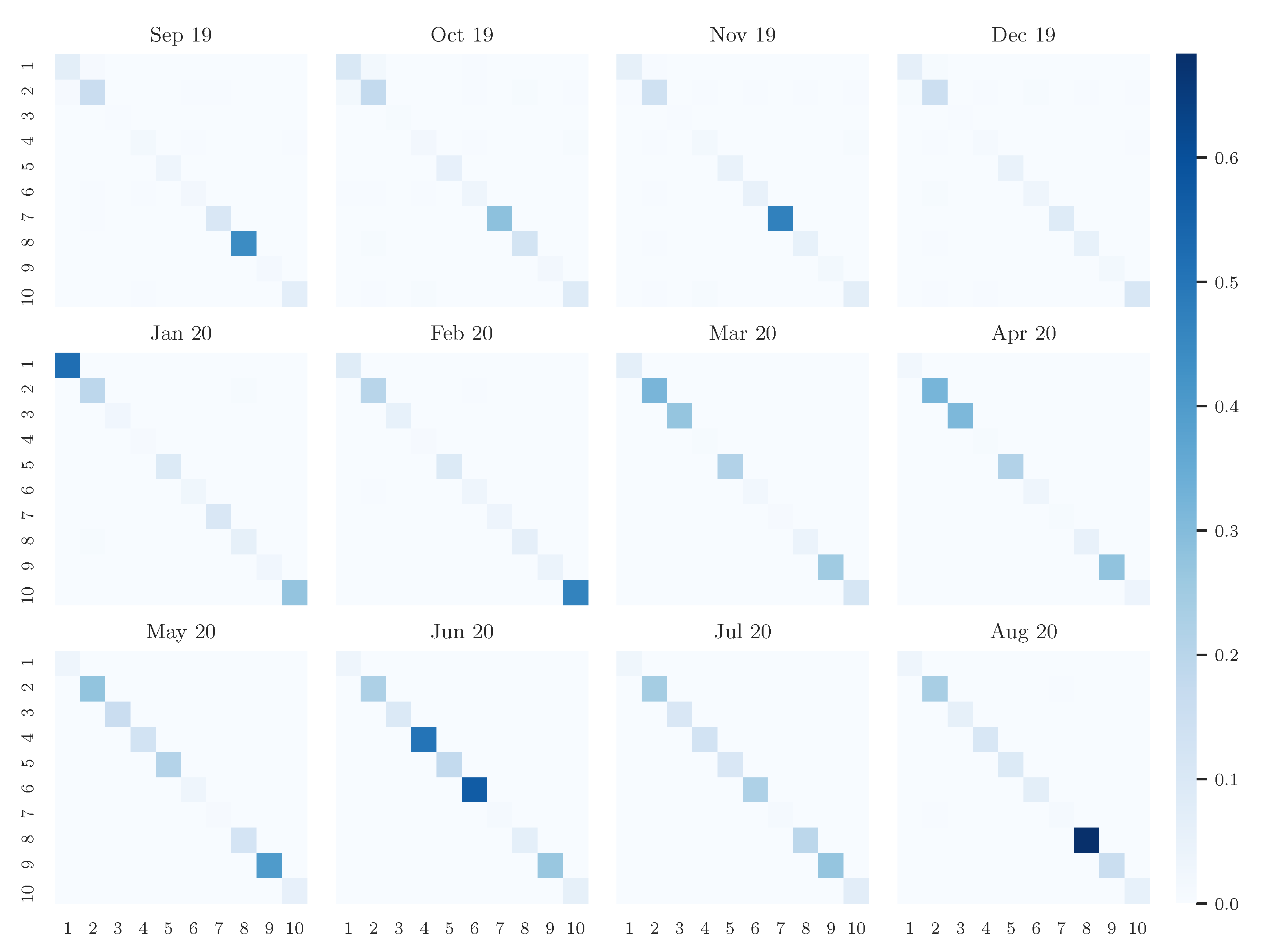
Appendix A.4. Additional Results on the New York Times News Article Data as Tensor Input
| Topic 1 | Topic 2 | Topic 3 | Topic 4 | Topic 5 | Topic 6 | Topic 7 | Topic 8 | Topic 9 | Topic 10 | |
|---|---|---|---|---|---|---|---|---|---|---|
| 0 | suleimani | loans | masks | floyd | contributed | confederate | ukraine | storm | restaurants | weinstein |
| (1.0) | (1.0) | (1.0) | (1.0) | (1.0) | (1.0) | (1.0) | (1.0) | (1.0) | (1.0) | |
| 1 | qassim | spend | sanitizer | brutality | alan | statue | lutsenko | storms | salons | raped |
| (1.0) | (1.0) | (1.0) | (1.0) | (1.0) | (1.0) | (1.0) | (1.0) | (1.0) | (1.0) | |
| 2 | iran | smallbusiness | wipes | police | edmondson | monuments | ukrainians | isaias | cafes | predatory |
| (1.0) | (1.0) | (1.0) | (1.0) | (1.0) | (1.0) | (1.0) | (1.0) | (1.0) | (1.0) | |
| 3 | iranian | rent | cloth | systemic | mervosh | statues | yovanovitch | landfall | pubs | mann |
| (1.0) | (1.0) | (1.0) | (1.0) | (1.0) | (1.0) | (1.0) | (1.0) | (1.0) | (1.0) | |
| 4 | militias | incentives | homemade | knee | emily | honoring | burisma | forecasters | nightclubs | sciorra |
| (1.0) | (1.0) | (1.0) | (1.0) | (1.0) | (1.0) | (1.0) | (1.0) | (1.0) | (1.0) | |
| 0 | iran | university | protective | minneapolis | reporting | statue | sondland | hurricane | bars | sexual |
| (1.0) | (1.0) | (1.0) | (1.0) | (1.0) | (1.0) | (1.0) | (1.0) | (1.0) | (1.0) | |
| 1 | qassim | jerome | gowns | breonna | rabin | monuments | zelensky | bahamas | dining | rape |
| (1.0) | (0.999) | (1.0) | (1.0) | (1.0) | (1.0) | (1.0) | (1.0) | (1.0) | (1.0) | |
| 2 | suleimani | oxford | ventilators | kueng | contributed | statues | volker | hurricanes | theaters | metoo |
| (1.0) | (0.998) | (1.0) | (1.0) | (1.0) | (1.0) | (1.0) | (1.0) | (1.0) | (1.0) | |
| 3 | iranian | columbia | respirators | floyd | keith | confederate | giuliani | forecasters | venues | sexually |
| (1.0) | (0.998) | (1.0) | (1.0) | (1.0) | (1.0) | (1.0) | (1.0) | (1.0) | (1.0) | |
| 4 | militias | economics | supplies | police | chokshi | honoring | quid | landfall | malls | mann |
| (1.0) | (0.998) | (1.0) | (1.0) | (1.0) | (1.0) | (1.0) | (1.0) | (1.0) | (1.0) |
| Topic 1 #977 | Topic 2 #360 | Topic 3 #420 | Topic 4 #4192 | Topic 5 #489 | Topic 6 #405 | Topic 7 #1135 | Topic 8 #748 | Topic 9 #108 | Topic 10 #1166 | |
|---|---|---|---|---|---|---|---|---|---|---|
| 1 | floyd | contributed | iran | masks | ship | syria | senator | restaurants | bloom | ukraine |
| (82.861) | (137.058) | (80.007) | (40.463) | (87.178) | (94.686) | (77.285) | (93.511) | (110.77) | (79.611) | |
| 2 | police | reporting | suleimani | patients | crew | syrian | storm | bars | julie | sondland |
| (64.649) | (84.889) | (78.78) | (34.77) | (70.694) | (82.565) | (43.439) | (64.889) | (103.282) | (61.099) | |
| 3 | protesters | michael | iranian | ventilators | aboard | kurdish | hurricane | reopen | edited | testimony |
| (63.588) | (76.156) | (72.581) | (34.299) | (67.464) | (82.013) | (42.213) | (57.541) | (100.159) | (49.982) | |
| 4 | minneapolis | katie | iraq | protective | passengers | turkey | iowa | stores | los | testified |
| (63.216) | (63.146) | (63.27) | (33.719) | (65.895) | (80.374) | (41.985) | (55.435) | (95.747) | (49.959) | |
| 5 | protests | emily | gen | loans | cruise | turkish | republican | gyms | graduated | zelensky |
| (61.585) | (60.696) | (50.966) | (28.178) | (63.535) | (75.912) | (40.993) | (50.487) | (93.51) | (48.427) | |
| 6 | george | alan | strike | supplies | princess | kurds | gov | theaters | angeles | ambassador |
| (53.378) | (59.499) | (49.026) | (27.15) | (45.714) | (63.639) | (37.689) | (49.866) | (92.349) | (46.086) | |
| 7 | brutality | nicholas | iraqi | gloves | flight | fighters | buttigieg | closed | berkeley | weinstein |
| (44.051) | (55.899) | (46.027) | (26.724) | (45.375) | (62.313) | (37.1) | (46.544) | (85.653) | (45.053) | |
| 8 | officers | cochrane | qassim | equipment | nasa | forces | democrat | indoor | grew | ukrainian |
| (43.581) | (52.045) | (45.861) | (26.252) | (43.306) | (57.659) | (37.087) | (44.541) | (84.145) | (43.716) | |
| 9 | racism | ben | maj | respiratory | navy | troops | representative | salons | today | giuliani |
| (43.457) | (41.414) | (44.921) | (25.447) | (40.396) | (54.045) | (35.807) | (41.99) | (41.818) | (42.674) | |
| 10 | demonstrations | maggie | baghdad | testing | astronauts | isis | bernie | shops | california | sexual |
| (42.547) | (41.328) | (44.867) | (24.179) | (37.073) | (53.743) | (35.228) | (40.311) | (38.807) | (39.966) |
| Topic 1 | Topic 2 | Topic 3 | Topic 4 | Topic 5 | Topic 6 | Topic 7 | Topic 8 | Topic 9 | Topic 10 | |
|---|---|---|---|---|---|---|---|---|---|---|
| 0 | floyd | contributed | iran | masks | ship | syria | senator | restaurants | bloom | ukraine |
| (1.0) | (1.0) | (1.0) | (1.0) | (1.0) | (1.0) | (1.0) | (1.0) | (1.0) | (1.0) | |
| 1 | demonstrations | shear | suleimani | providers | aboard | isis | wyden | shops | graduated | volker |
| (1.0) | (1.0) | (1.0) | (1.0) | (1.0) | (1.0) | (1.0) | (1.0) | (1.0) | (1.0) | |
| 2 | systemic | annie | retaliation | distressed | capsule | ceasefire | iowa | takeout | edited | inquiry |
| (1.0) | (1.0) | (1.0) | (1.0) | (1.0) | (0.999) | (1.0) | (1.0) | (1.0) | (1.0) | |
| 3 | protests | mazzei | qassim | tobacco | diamond | fighters | steyer | nightclubs | berkeley | transcript |
| (1.0) | (1.0) | (1.0) | (1.0) | (1.0) | (0.999) | (1.0) | (1.0) | (1.0) | (1.0) | |
| 4 | defund | kitty | revenge | selfemployed | dragon | syrian | klobuchar | pubs | grew | investigations |
| (1.0) | (1.0) | (1.0) | (1.0) | (1.0) | (0.999) | (1.0) | (1.0) | (1.0) | (1.0) | |
| 0 | police | reporting | suleimani | patients | crew | syrian | storm | bars | julie | sondland |
| (1.0) | (1.0) | (1.0) | (1.0) | (1.0) | (1.0) | (1.0) | (1.0) | (1.0) | (1.0) | |
| 1 | systemic | luis | strike | treating | aboard | alassad | carolina | reopen | garcetti | testifying |
| (1.0) | (1.0) | (1.0) | (1.0) | (1.0) | (1.0) | (1.0) | (1.0) | (0.993) | (1.0) | |
| 2 | peaceful | beachy | maj | infection | capsule | recep | rubio | nonessential | graduated | mick |
| (1.0) | (1.0) | (1.0) | (1.0) | (1.0) | (1.0) | (1.0) | (1.0) | (0.988) | (1.0) | |
| 3 | peacefully | kaplan | iran | develop | princess | erdogan | hampshire | nail | edited | quid |
| (1.0) | (1.0) | (1.0) | (1.0) | (1.0) | (1.0) | (1.0) | (1.0) | (0.988) | (1.0) | |
| 4 | knee | glueck | retaliation | repay | cruise | kurds | landfall | takeout | berkeley | impeachment |
| (1.0) | (1.0) | (1.0) | (1.0) | (1.0) | (1.0) | (1.0) | (1.0) | (0.988) | (1.0) |


Appendix B. Matrix Derivatives
References
- Levy, O.; Goldberg, Y. Neural Word Embedding as Implicit Matrix Factorization. In Advances in Neural Information Processing Systems; NIPS’14; MIT Press: Cambridge, MA, USA, 2014; Volume 2, pp. 2177–2185. [Google Scholar]
- Pennington, J.; Socher, R.; Manning, C. Glove: Global Vectors for Word Representation. In Proceedings of the 2014 Conference on Empirical Methods in Natural Language Processing (EMNLP), Association for Computational Linguistics, Doha, Qatar, 25–29 October 2014; pp. 1532–1543. [Google Scholar]
- Hillebrand, L.P.; Biesner, D.; Bauckhage, C.; Sifa, R. Interpretable Topic Extraction and Word Embedding Learning Using Row-Stochastic DEDICOM. In Machine Learning and Knowledge Extraction—4th International Cross-Domain Conference, CD-MAKE; Lecture Notes in Computer Science; Springer: Dublin, Ireland, 2020; Volume 12279, pp. 401–422. [Google Scholar]
- Symeonidis, P.; Zioupos, A. Matrix and Tensor Factorization Techniques for Recommender Systems; Springer International Publishing: New York, NY, USA, 2016. [Google Scholar] [CrossRef]
- Harshman, R.; Green, P.; Wind, Y.; Lundy, M. A Model for the Analysis of Asymmetric Data in Marketing Research. Market. Sci. 1982, 1, 205–242. [Google Scholar] [CrossRef]
- Andrzej, A.H.; Cichocki, A.; Dinh, T.V. Nonnegative DEDICOM Based on Tensor Decompositions for Social Networks Exploration. Aust. J. Intell. Inf. Process. Syst. 2010, 12, 10–15. [Google Scholar]
- Bader, B.W.; Harshman, R.A.; Kolda, T.G. Pattern Analysis of Directed Graphs Using DEDICOM: An Application to Enron Email; Office of Scientific & Technical Information Technical Reports; Sandia National Laboratories: Albuquerque, NM, USA, 2006. [Google Scholar]
- Sifa, R.; Ojeda, C.; Cvejoski, K.; Bauckhage, C. Interpretable Matrix Factorization with Stochasticity Constrained Nonnegative DEDICOM. In Proceedings of the KDML-LWDA, Rostock, Germany, 11–13 September 2017. [Google Scholar]
- Sifa, R.; Ojeda, C.; Bauckage, C. User Churn Migration Analysis with DEDICOM. In Proceedings of the 9th ACM Conference on Recommender Systems; RecSys ’15; Association for Computing Machinery: New York, NY, USA, 2015; pp. 321–324. [Google Scholar]
- Chew, P.; Bader, B.; Rozovskaya, A. Using DEDICOM for Completely Unsupervised Part-of-Speech Tagging. In Proceedings of the Workshop on Unsupervised and Minimally Supervised Learning of Lexical Semantics, Boulder, CO, USA, 5 June 2009; Association for Computational Linguistics: Boulder, CO, USA, 2009; pp. 54–62. [Google Scholar]
- Nickel, M.; Tresp, V.; Kriegel, H.P. A Three-Way Model for Collective Learning on Multi-Relational Data. In Proceedings of the 28th International Conference on Machine Learning, Bellevue, WA, USA, 28 June–2 July 2009; Association for Computing Machinery: Bellevue, WA, USA, 2011; pp. 809–816. [Google Scholar]
- Sifa, R.; Yawar, R.; Ramamurthy, R.; Bauckhage, C.; Kersting, K. Matrix- and Tensor Factorization for Game Content Recommendation. KI-Künstl. Intell. 2019, 34, 57–67. [Google Scholar] [CrossRef]
- Mikolov, T.; Sutskever, I.; Chen, K.; Corrado, G.; Dean, J. Distributed Representations of Words and Phrases and their Compositionality. Adv. Neural Inf. Proc. Syst. 2013, arXiv:cs.CL/1310.454626, 3111–3119. [Google Scholar]
- Lee, D.D.; Seung, H.S. Algorithms for Non-Negative Matrix Factorization. In Proceedings of the 13th International Conference on Neural Information Processing Systems; NIPS’00; MIT Press: Cambridge, MA, USA, 2000; pp. 535–541. [Google Scholar]
- Furnas, G.W.; Deerwester, S.; Dumais, S.T.; Landauer, T.K.; Harshman, R.A.; Streeter, L.A.; Lochbaum, K.E. Information Retrieval Using a Singular Value Decomposition Model of Latent Semantic Structure. In ACM SIGIR Forum; ACM: New York, NY, USA, 1988. [Google Scholar]
- Wang, Y.; Zhu, L. Research and implementation of SVD in machine learning. In Proceedings of the 2017 IEEE/ACIS 16th International Conference on Computer and Information Science (ICIS), Wuhan, China, 24–26 May 2017; pp. 471–475. [Google Scholar]
- Jolliffe, I. Principal Component Analysis; John Wiley and Sons Ltd.: Hoboken, NJ, USA, 2005. [Google Scholar]
- Blei, D.M.; Ng, A.Y.; Jordan, M.I. Latent Dirichlet Allocation. J. Mach. Learn. Res. 2003, 3, 993–1022. [Google Scholar]
- Lebret, R.; Collobert, R. Word Embeddings through Hellinger PCA. In Proceedings of the 14th Conference of the European Chapter of the Association for Computational Linguistics, Gothenburg, Sweden, 26–30 April 2014; pp. 482–490. [Google Scholar]
- Nguyen, D.Q.; Billingsley, R.; Du, L.; Johnson, M. Improving Topic Models with Latent Feature Word Representations. Trans. Assoc. Comput. Linguist. 2015, 3, 299–313. [Google Scholar] [CrossRef]
- Frank, M.; Wolfe, P. An algorithm for quadratic programming. Naval Res. Logist. Q. 1956, 3, 95–110. [Google Scholar] [CrossRef]
- Ni, J.; Li, J.; McAuley, J. Justifying recommendations using distantly-labeled reviews and fine-grained aspects. In Proceedings of the 2019 Conference on Empirical Methods in Natural Language Processing and the 9th International Joint Conference on Natural Language Processing (EMNLP-IJCNLP), Hong Kong, China, 3–7 November 2019; pp. 188–197. [Google Scholar]
- Kingma, D.P.; Ba, J. Adam: A method for stochastic optimization. arXiv 2014, arXiv:1412.6980. [Google Scholar]
- McInnes, L.; Healy, J.; Melville, J. UMAP: Uniform Manifold Approximation and Projection for Dimension Reduction. arXiv 2018, arXiv:1802.03426. [Google Scholar]


| Movie | # Reviews |
|---|---|
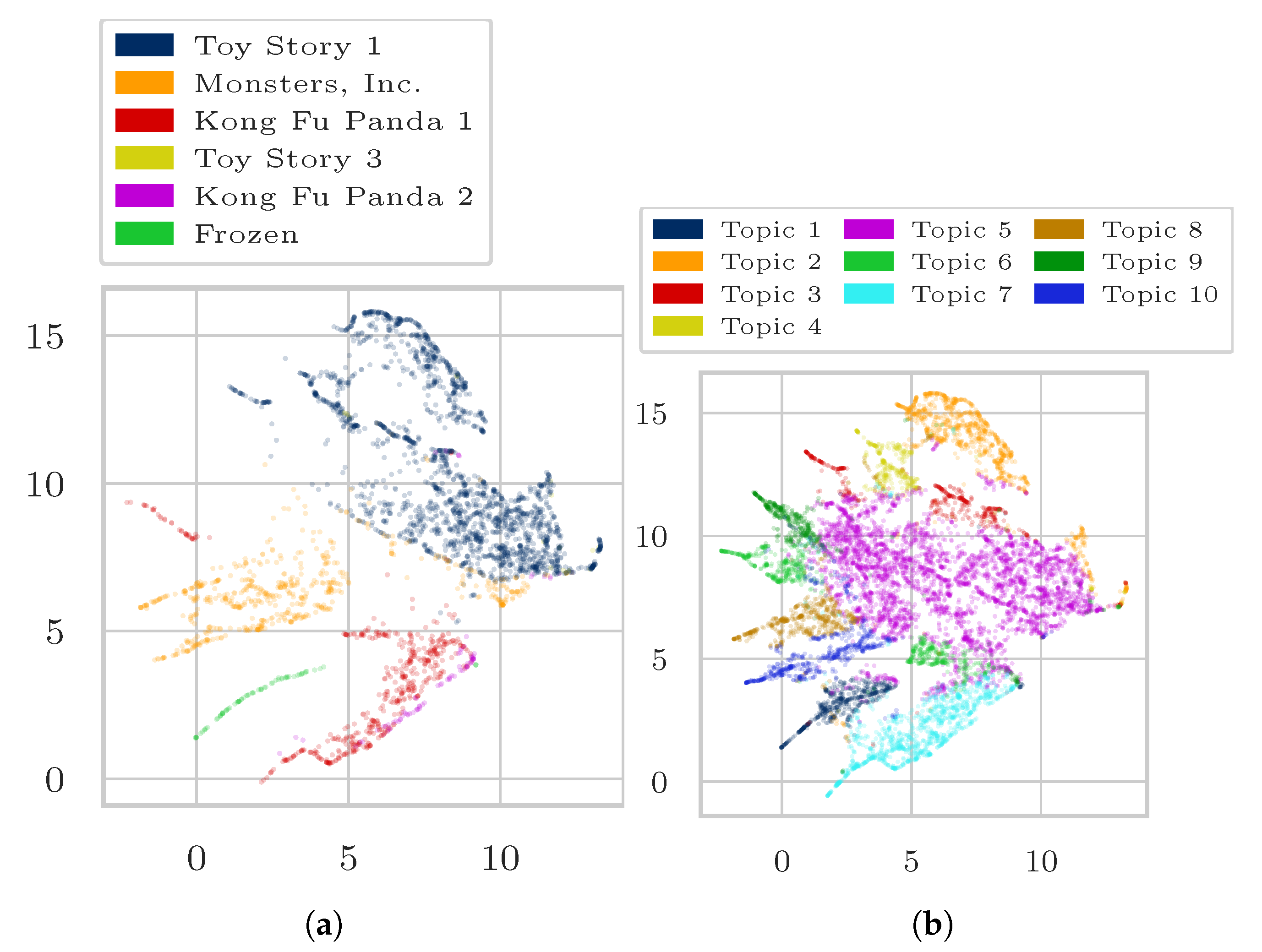
| Toy Story 1 | 2491 |
| Monsters, Inc. | 3203 |
| Kung Fu Panda 1 | 6708 |
| Toy Story 3 | 1209 |
| Kung Fu Panda 2 | 1208 |
| Frozen | 1292 |
| Section | # Articles |
|---|---|
| Politics | 3204 |
| U.S. | 2610 |
| Business | 1624 |
| New York | 1528 |
| Europe | 988 |
| Asia Pacific | 839 |
| Health | 598 |
| Technology | 551 |
| Middle East | 443 |
| Science | 440 |
| Economy | 339 |
| Elections | 240 |
| Climate | 239 |
| World | 233 |
| Africa | 124 |
| Australia | 113 |
| Canada | 104 |
| Month | # Articles |
|---|---|
| September 2019 | 1586 |
| October 2019 | 1788 |
| November 2019 | 1623 |
| December 2019 | 1461 |
| January 2020 | 1725 |
| Febuary 2020 | 1602 |
| March 2020 | 1937 |
| April 2020 | 1712 |
| May 2020 | 1713 |
| June 2020 | 1828 |
| July 2020 | 1814 |
| August 2020 | 1886 |
| Total | Unique | Avg. Total | Avg Unique | Cutoff | |
|---|---|---|---|---|---|
| Amazon Reviews | 252,400 | 15,560 | 15.2 | 13.4 | 1 |
| Wikipedia DSW | 14,500 | 4376 | 4833.3 | 2106.0 | 1 |
| Wikipedia SBJ | 10,435 | 4034 | 3478.3 | 1600.3 | 1 |
| Wikipedia STR | 11,501 | 3224 | 3833.7 | 1408.0 | 1 |
| New York Times | 12,043,205 | 141,591 | 582.5 | 366.5 | 118 |
| Topic 1 #619 | Topic 2 #1238 | Topic 3 #628 | Topic 4 #595 | Topic 5 #612 | Topic 6 #389 | |
|---|---|---|---|---|---|---|
| 1 | ball | film | salazar | cup | bees | heard |
| (0.77) | (0.857) | (0.201) | (0.792) | (0.851) | (0.738) | |
| 2 | penalty | starred | geoffrey | football | species | court |
| (0.708) | (0.613) | (0.2) | (0.745) | (0.771) | (0.512) | |
| 3 | may | role | rush | fifa | bee | depp |
| (0.703) | (0.577) | (0.2) | (0.731) | (0.753) | (0.505) | |
| 4 | referee | series | brenton | world | pollen | divorce |
| (0.667) | (0.504) | (0.199) | (0.713) | (0.658) | (0.454) | |
| 5 | goal | burton | hardwicke | national | honey | alcohol |
| (0.66) | (0.492) | (0.198) | (0.639) | (0.602) | (0.435) | |
| 6 | team | character | thwaites | uefa | insects | paradis |
| (0.651) | (0.465) | (0.198) | (0.623) | (0.576) | (0.42) | |
| 7 | players | played | catherine | continental | food | relationship |
| (0.643) | (0.451) | (0.198) | (0.582) | (0.536) | (0.419) | |
| 8 | player | director | kaya | teams | nests | abuse |
| (0.639) | (0.45) | (0.198) | (0.576) | (0.529) | (0.41) | |
| 9 | play | success | melfi | european | solitary | stating |
| (0.606) | (0.438) | (0.198) | (0.57) | (0.513) | (0.408) | |
| 10 | game | jack | raimi | association | eusocial | stated |
| (0.591) | (0.434) | (0.198) | (0.563) | (0.505) | (0.402) |
| Topic 1 | Topic 2 | Topic 3 | Topic 4 | Topic 5 | Topic 6 | |
|---|---|---|---|---|---|---|
| 0 | ball | film | salazar | cup | bees | heard |
| (1.0) | (1.0) | (1.0) | (1.0) | (1.0) | (1.0) | |
| 1 | penalty | starred | geoffrey | fifa | bee | court |
| (0.994) | (0.978) | (1.0) | (0.995) | (0.996) | (0.966) | |
| 2 | referee | role | rush | national | species | divorce |
| (0.992) | (0.964) | (1.0) | (0.991) | (0.995) | (0.944) | |
| 3 | may | burton | bardem | world | pollen | alcohol |
| (0.989) | (0.937) | (1.0) | (0.988) | (0.986) | (0.933) | |
| 4 | goal | series | brenton | uefa | honey | abuse |
| (0.986) | (0.935) | (1.0) | (0.987) | (0.971) | (0.914) | |
| 0 | penalty | starred | geoffrey | football | species | court |
| (1.0) | (1.0) | (1.0) | (1.0) | (1.0) | (1.0) | |
| 1 | referee | role | rush | fifa | bees | divorce |
| (0.999) | (0.994) | (1.0) | (0.994) | (0.995) | (0.995) | |
| 2 | goal | series | salazar | national | bee | alcohol |
| (0.998) | (0.985) | (1.0) | (0.983) | (0.99) | (0.987) | |
| 3 | player | burton | brenton | cup | pollen | abuse |
| (0.997) | (0.981) | (1.0) | (0.983) | (0.99) | (0.982) | |
| 4 | ball | film | thwaites | world | insects | settlement |
| (0.994) | (0.978) | (1.0) | (0.982) | (0.977) | (0.978) |
| Topic 1 #481 | Topic 2 #661 | Topic 3 #414 | Topic 4 #457 | Topic 5 #316 | Topic 6 #1711 | |
|---|---|---|---|---|---|---|
| 1 | hind | game | film | heard | bees | disorder |
| (0.646) | (0.83) | (0.941) | (0.844) | (0.922) | (0.291) | |
| 2 | segments | football | starred | court | bee | collapse |
| (0.572) | (0.828) | (0.684) | (0.566) | (0.868) | (0.29) | |
| 3 | bacteria | players | role | divorce | honey | attrition |
| (0.563) | (0.782) | (0.624) | (0.51) | (0.756) | (0.285) | |
| 4 | legs | ball | series | depp | insects | losses |
| (0.562) | (0.777) | (0.562) | (0.508) | (0.68) | (0.284) | |
| 5 | antennae | team | burton | sued | food | invertebrate |
| (0.555) | (0.771) | (0.547) | (0.48) | (0.634) | (0.283) | |
| 6 | females | may | character | stating | species | rate |
| (0.549) | (0.696) | (0.499) | (0.45) | (0.599) | (0.283) | |
| 7 | wings | play | success | alcohol | nests | businesses |
| (0.547) | (0.692) | (0.494) | (0.449) | (0.596) | (0.282) | |
| 8 | small | competitions | played | paradis | flowers | virgil |
| (0.538) | (0.677) | (0.483) | (0.446) | (0.571) | (0.282) | |
| 9 | groups | match | films | alleged | pollen | iridescent |
| (0.527) | (0.672) | (0.482) | (0.445) | (0.56) | (0.282) | |
| 10 | males | penalty | box | stated | larvae | detail |
| (0.518) | (0.664) | (0.465) | (0.444) | (0.529) | (0.281) |
| Topic 1 #521 | Topic 2 #249 | Topic 3 #485 | Topic 4 #871 | Topic 5 #445 | Topic 6 #1469 | |
|---|---|---|---|---|---|---|
| 1 | species | game | honey | allow | insects | depp |
| (3.105) | (3.26) | (2.946) | (0.668) | (2.794) | (2.419) | |
| 2 | eusocial | football | bee | organised | pollen | film |
| (2.524) | (3.05) | (2.01) | (0.662) | (2.239) | (2.115) | |
| 3 | solitary | players | beekeeping | winner | flowers | role |
| (2.279) | (2.699) | (1.933) | (0.632) | (2.019) | (1.32) | |
| 4 | nest | ball | bees | officially | nectar | starred |
| (2.118) | (2.475) | (1.704) | (0.626) | (1.656) | (1.3) | |
| 5 | females | may | increased | wins | wasps | actor |
| (1.993) | (2.447) | (1.589) | (0.617) | (1.602) | (1.155) | |
| 6 | workers | team | humans | level | wings | series |
| (1.797) | (2.424) | (1.515) | (0.613) | (1.588) | (1.126) | |
| 7 | nests | association | wild | free | many | burton |
| (1.787) | (1.92) | (1.415) | (0.6) | (1.588) | (1.112) | |
| 8 | colonies | play | mites | constitute | hind | played |
| (1.722) | (1.834) | (1.4) | (0.596) | (1.577) | (1.068) | |
| 9 | egg | referee | colony | regulation | hairs | heard |
| (1.692) | (1.809) | (1.35) | (0.595) | (1.484) | (1.005) | |
| 10 | males | laws | beekeepers | prestigious | pollinating | success |
| (1.664) | (1.792) | (1.332) | (0.594) | (1.467) | (0.981) |
| Topic 1 | Topic 2 | Topic 3 | Topic 4 | Topic 5 | Topic 6 | |
|---|---|---|---|---|---|---|
| 0 | hind | game | film | heard | bees | disorder |
| (1.0) | (1.0) | (1.0) | (1.0) | (1.0) | (1.0) | |
| 1 | segments | football | starred | court | bee | collapse |
| (0.995) | (1.0) | (0.968) | (0.954) | (0.999) | (1.0) | |
| 2 | legs | players | role | divorce | honey | losses |
| (0.994) | (0.999) | (0.954) | (0.925) | (0.99) | (1.0) | |
| 3 | antennae | ball | series | sued | insects | attrition |
| (0.993) | (0.999) | (0.951) | (0.907) | (0.976) | (0.999) | |
| 4 | wings | team | burton | alleged | food | businesses |
| (0.992) | (0.998) | (0.945) | (0.897) | (0.97) | (0.999) | |
| 0 | segments | football | starred | court | bee | collapse |
| (1.0) | (1.0) | (1.0) | (1.0) | (1.0) | (1.0) | |
| 1 | antennae | game | role | divorce | bees | disorder |
| (1.0) | (1.0) | (0.993) | (0.996) | (0.999) | (1.0) | |
| 2 | wings | players | series | sued | honey | losses |
| (0.999) | (0.999) | (0.978) | (0.991) | (0.995) | (0.999) | |
| 3 | bacteria | ball | burton | alleged | insects | pesticide |
| (0.999) | (0.999) | (0.975) | (0.981) | (0.984) | (0.998) | |
| 4 | legs | team | film | alcohol | food | businesses |
| (0.998) | (0.999) | (0.968) | (0.981) | (0.976) | (0.998) |
| Topic 1 | Topic 2 | Topic 3 | Topic 4 | Topic 5 | Topic 6 | |
|---|---|---|---|---|---|---|
| 0 | species | game | honey | allow | insects | depp |
| (1.0) | (1.0) | (1.0) | (1.0) | (1.0) | (1.0) | |
| 1 | easier | football | boatwrights | emancipation | ultraviolet | charlie |
| (1.0) | (1.0) | (1.0) | (1.0) | (1.0) | (1.0) | |
| 2 | tiny | players | glade | broadly | mechanics | infiltrate |
| (1.0) | (1.0) | (1.0) | (1.0) | (1.0) | (1.0) | |
| 3 | halictidae | association | tutankhamun | disabilities | exploit | thenwife |
| (0.999) | (1.0) | (1.0) | (1.0) | (1.0) | (1.0) | |
| 4 | provision | team | oracle | total | swallows | tourist |
| (0.999) | (0.997) | (1.0) | (1.0) | (1.0) | (1.0) | |
| 0 | eusocial | football | bee | organised | pollen | film |
| (1.0) | (1.0) | (1.0) | (1.0) | (1.0) | (1.0) | |
| 1 | oligocene | players | subfamilies | comes | honeybees | starred |
| (1.0) | (1.0) | (0.995) | (1.0) | (1.0) | (1.0) | |
| 2 | architecture | game | internal | shows | enlarged | smoking |
| (1.0) | (1.0) | (0.994) | (1.0) | (0.998) | (0.999) | |
| 3 | uncommon | association | studied | attention | simple | dislocated |
| (1.0) | (1.0) | (0.994) | (1.0) | (0.998) | (0.999) | |
| 4 | termed | team | cladogram | deductions | drove | injuries |
| (1.0) | (0.997) | (0.99) | (1.0) | (0.998) | (0.999) |
| Topic 1 #528 | Topic 2 #445 | Topic 3 #1477 | Topic 4 #1790 | Topic 5 #1917 | Topic 6 #597 | Topic 7 #789 | Topic 8 #670 | Topic 9 #1599 | Topic 10 #188 | |
|---|---|---|---|---|---|---|---|---|---|---|
| 1 | anna | shen | legendary | lasseter | disc | screams | code | mike | woody | po |
| (4.215) | (4.21) | (1.459) | (2.887) | (1.367) | (3.779) | (3.292) | (4.325) | (6.12) | (5.737) | |
| 2 | elsa | peacock | valley | director | birds | energy | crystal | buzz | master | |
| (4.087) | (2.668) | (1.448) | (2.392) | (1.343) | (3.315) | (2.781) | (4.055) | (5.484) | (5.276) | |
| 3 | olaf | oldman | temple | andrew | widescreen | monstropolis | promo | billy | andy | shifu |
| (2.315) | (2.627) | (1.31) | (2.158) | (1.327) | (3.13) | (2.645) | (3.911) | (4.355) | (4.707) | |
| 4 | trolls | gary | kim | stanton | outtakes | world | free | goodman | toys | dragon |
| (2.241) | (2.423) | (1.307) | (2.119) | (1.238) | (3.109) | (2.343) | (3.812) | (4.119) | (4.344) | |
| 5 | frozen | lord | fearsome | special | extras | monsters | promotion | sully | lightyear | warrior |
| (2.196) | (2.201) | (1.288) | (1.892) | (1.185) | (3.047) | (2.279) | (3.728) | (3.334) | (4.274) | |
| 6 | kristoff | weapon | teacher | pete | dvd | city | promotional | wazowski | allen | tai |
| (2.155) | (1.469) | (1.288) | (1.612) | (1.142) | (2.994) | (2.266) | (3.513) | (2.752) | (4.082) | |
| 7 | queen | wolf | battle | ranft | included | monster | amazon | randall | tim | lung |
| (2.055) | (1.405) | (1.264) | (1.564) | (1.13) | (2.978) | (2.129) | (3.404) | (2.609) | (3.993) | |
| 8 | hans | inner | duk | joe | short | power | click | sulley | hanks | five |
| (2.054) | (1.38) | (1.257) | (1.564) | (1.101) | (2.919) | (2.024) | (3.396) | (2.471) | (2.952) | |
| 9 | sister | yeoh | train | feature | games | scare | download | buscemi | cowboy | oogway |
| (1.904) | (1.359) | (1.221) | (1.555) | (1.1) | (2.614) | (1.889) | (3.266) | (2.407) | (2.918) | |
| 10 | ice | michelle | warriors | ralph | tour | closet | instructions | james | space | furious |
| (1.839) | (1.354) | (1.22) | (1.518) | (1.031) | (2.555) | (1.877) | (3.264) | (2.375) | (2.806) |
| Topic 1 #454 | Topic 2 #5984 | Topic 3 #567 | Topic 4 #562 | Topic 5 #424 | Topic 6 #330 | Topic 7 #515 | Topic 8 #297 | Topic 9 #431 | Topic 10 #436 | |
|---|---|---|---|---|---|---|---|---|---|---|
| 1 | suleimani | loans | masks | floyd | contributed | confederate | ukraine | storm | restaurants | weinstein |
| (2.812) | (0.618) | (3.261) | (3.376) | (4.565) | (3.226) | (3.191) | (2.76) | (2.948) | (3.442) | |
| 2 | iran | university | protective | minneapolis | reporting | statue | sondland | hurricane | bars | sexual |
| (2.593) | (0.551) | (2.823) | (2.551) | (2.788) | (2.649) | (2.881) | (2.622) | (2.021) | (2.71) | |
| 3 | iraq | oil | gloves | police | michael | statues | zelensky | winds | reopen | rape |
| (2.453) | (0.549) | (2.516) | (2.255) | (2.707) | (2.416) | (2.133) | (1.715) | (1.684) | (2.102) | |
| 4 | iranian | billion | ventilators | george | katie | monuments | ambassador | tropical | gyms | assault |
| (2.408) | (0.54) | (2.22) | (2.088) | (2.324) | (1.815) | (1.976) | (1.606) | (1.654) | (1.861) | |
| 5 | iraqi | loan | surgical | protests | alan | monument | ukrainian | storms | stores | jury |
| (1.799) | (0.468) | (2.032) | (1.936) | (2.292) | (1.375) | (1.789) | (1.439) | (1.638) | (1.513) | |
| 6 | baghdad | bonds | gowns | brutality | emily | flag | giuliani | coast | theaters | charges |
| (1.604) | (0.466) | (1.965) | (1.765) | (2.165) | (1.206) | (1.755) | (1.415) | (1.627) | (1.409) | |
| 7 | qassim | payments | equipment | racism | nicholas | richmond | volker | laura | salons | predatory |
| (1.599) | (0.456) | (1.86) | (1.579) | (2.096) | (1.109) | (1.754) | (1.259) | (1.438) | (1.387) | |
| 8 | strike | edited | supplies | knee | cochrane | symbols | investigations | isaias | closed | harvey |
| (1.597) | (0.452) | (1.816) | (1.435) | (1.934) | (1.089) | (1.602) | (1.217) | (1.424) | (1.35) | |
| 9 | gen | trillion | gear | killing | rappeport | remove | testified | category | shops | guilty |
| (1.513) | (0.451) | (1.742) | (1.429) | (1.613) | (1.058) | (1.584) | (1.192) | (1.325) | (1.312) | |
| 10 | maj | graduated | mask | officers | maggie | removal | testimony | landfall | indoor | sex |
| (1.504) | (0.449) | (1.502) | (1.405) | (1.529) | (1.003) | (1.558) | (1.106) | (1.247) | (1.3) |
Publisher’s Note: MDPI stays neutral with regard to jurisdictional claims in published maps and institutional affiliations. |
© 2021 by the authors. Licensee MDPI, Basel, Switzerland. This article is an open access article distributed under the terms and conditions of the Creative Commons Attribution (CC BY) license (http://creativecommons.org/licenses/by/4.0/).
Share and Cite
Hillebrand, L.; Biesner, D.; Bauckhage, C.; Sifa, R. Interpretable Topic Extraction and Word Embedding Learning Using Non-Negative Tensor DEDICOM. Mach. Learn. Knowl. Extr. 2021, 3, 123-167. https://doi.org/10.3390/make3010007
Hillebrand L, Biesner D, Bauckhage C, Sifa R. Interpretable Topic Extraction and Word Embedding Learning Using Non-Negative Tensor DEDICOM. Machine Learning and Knowledge Extraction. 2021; 3(1):123-167. https://doi.org/10.3390/make3010007
Chicago/Turabian StyleHillebrand, Lars, David Biesner, Christian Bauckhage, and Rafet Sifa. 2021. "Interpretable Topic Extraction and Word Embedding Learning Using Non-Negative Tensor DEDICOM" Machine Learning and Knowledge Extraction 3, no. 1: 123-167. https://doi.org/10.3390/make3010007
APA StyleHillebrand, L., Biesner, D., Bauckhage, C., & Sifa, R. (2021). Interpretable Topic Extraction and Word Embedding Learning Using Non-Negative Tensor DEDICOM. Machine Learning and Knowledge Extraction, 3(1), 123-167. https://doi.org/10.3390/make3010007